Metal abundances of RR Lyrae stars in the bar of the Large Magellanic Cloud

Metallicities ([Fe/H]) from low resolution spectroscopy obtained with the Very Large Telescope (VLT) are presented for 98 RR Lyrae and 3 short period Cepheids in the bar of the Large Magellanic Cloud. Our metal abundances have typical errors of $\pm 0.17$ dex. The average metallicity of the RR Lyrae stars is [Fe/H]=$-1.48\pm 0.03\pm 0.06$ on the scale of Harris (1996). The star-to-star scatter (0.29 dex) is larger than the observational errors, indicating a real spread in metal abundances. The derived metallicities cover the range $-2.12<$[Fe/H]$<-0.27$, but there are only a few stars having [Fe/H]$>-1$. For the $ab-$type variables we compared our spectroscopic abundances with those obtained from the Fourier decomposition of the light curves. We find good agreement between the two techniques, once the systematic offset of 0.2 dex between the metallicity scales used in the two methods is taken into account. The spectroscopic metallicities were combined with the dereddened apparent magnitudes of the variables to derive the slope of the luminosity-metallicity relation for the LMC RR Lyrae stars: the resulting value is $0.214\pm 0.047$ mag/dex. Finally, the 3 short period Cepheids have [Fe/H] values in the range $-2.0<$[Fe/H]$<-1.5$. They are more metal-poor than typical LMC RR Lyrae stars, thus they are more likely to be Anomalous Cepheids rather than the short period Classical Cepheids that are being found in a number of dwarf Irregular galaxies.

1 Introduction

The Large Magellanic Cloud (LMC) is a first step in our knowledge of the extragalactic astronomical distance scale. A variety of distance estimates to the LMC have been published in recent years (for references, see Clementini et al. 2003a). Among those based on Population II indicators, most are tied to the value of the absolute visual magnitude of the RR Lyrae variables, that is the radial pulsators within the classic instability strip on the core He-burning phase of the metal-poor stars (the so-called horizontal branch, HB). The mean intrinsic luminosity of the RR Lyrae stars depends on metallicity according to a relation often assumed to be linear: $M_{V}(RR)=\alpha{\rm[Fe/H]}+\beta$ (Sandage 1981a,b), and, at fixed metal abundance, it is also slightly dependent on evolution off the Zero Age Horizontal Branch (ZAHB; Sandage 1990).

The precise form of the $M_{V}(RR)-$[Fe/H] relationship is still matter of debate; and while growing consensus is being reached on its zero point ($\beta\sim 0.6$ mag at [Fe/H]=$-1.5$, Cacciari & Clementini 2003, and references therein), there is still disagreement on the value of the slope since literature values range from 0.30 to 0.18-0.20 mag/dex (Cacciari 1999, Carretta et al. 2000). It has even been suggested that $\alpha$ may not be unique on the metallicity range spanned by the Galactic globular clusters (GGCs) since two different linear relationships would be followed by the metal-poor ([Fe/H]$<-1.5$) and the metal-rich ([Fe/H]$>-1.5$) Galactic and LMC cluster RR Lyrae stars (Rey et al. 2000, Caputo et al. 2000).

Sandage (1993a) found a rather steep slope of the $M_{V}(RR)-$[Fe/H] relationship $\alpha\sim 0.30$ mag/dex from the from the so-called period-shift analysis of the RR Lyrae stars in a number of Galactic globular clusters.

The theoretical evolutionary and pulsation models of horizontal branch (HB) stars favour instead a shallower slope $\alpha\sim 0.2$ mag/dex, and also provide evidence for a non-linearity that makes the relation steeper for more metal rich stars, as recently reviewed and summarized by Cacciari & Clementini (2003). A mild slope was also found from the Baade-Wesselink method applied to Galactic field RR Lyrae stars (Fernley et al. 1998), and from the determination of the magnitude of the HB in globular clusters of M31 (Rich et al. 2001), However both these studies do not find clear evidence for a break at [Fe/H]=$-1.5$, thus raising concerns on the actual universality of the HB luminosity-metallicity relationship.

The slope of the luminosity-metallicity relation of the RR Lyrae stars can provide clues on the Galactic globular clusters relative ages and on the time scale of the Galactic halo formation and early evolution. In fact, given the almost constant difference in luminosity between Turn-Off and HB stars: $\Delta{\rm V}^{\rm HB}_{\rm TO}$, found for the GGCs, if $\alpha$ is as steep as $\sim 0.3$ mag/dex, globular clusters of different metallicities would be coeval; while if it is $\sim 0.2$, the most metal-rich globular clusters like 47 Tuc would be $\sim 2-3$ Gyr younger than the most metal-poor ones (Sandage 1993b, and references therein).

Furthermore, the entire Population II distance scale would be affected if the $M_{V}(RR)-$[Fe/H] relation was found to be not universal and depending instead on the star formation history and the environment conditions of the host galaxy.

It is thus important to derive the luminosity-metallicity relationship for RR Lyrae stars in different extragalactic systems, the LMC in particular. Walker (1992a) presented both photometry and metallicity estimates (based on the color magnitude diagrams and the properties of the RR Lyrae variables) for the LMC globular clusters known to host RR Lyraes, which however are only a few (7) and cover a small range in metal abundance ($-2.3<{\rm[Fe/H]}<-1.7$, Walker 1992a, and references therein). Furthermore, these clusters are spread over a wide region of the sky, and some of them may well be at distances somewhat different from the average of the LMC: given the small numbers involved, uncertainties related to the depth of the LMC may be as large as about 0.1 mag. More recently, several thousands field RR Lyrae variables have been identified in the Clouds by surveys devoted to the detection of microlensing events (MACHO: Alcock et al. 1996; OGLE: Udalski et al. 1997). However, metallicity estimates are available so far only for a handful of them (Alcock et al. 1996). If we combine the depth uncertainties with possible evolution off the ZAHB, at least 100 variables are needed to obtain an accuracy of 0.05 mag/dex in the slope of the luminosity-metallicity relation.

In recent years we began a study of the RR Lyrae variables in two fields close to the bar of the LMC. Our initial aim was to derive the mass-metallicity relation for the double mode pulsators (RRd), described in an earlier paper (Bragaglia et al. 2001). Accurate photometry for these fields in the Johnson $BV$ and Cousins $I$ bands was obtained using the Danish 1.5 m telescope, and spectroscopy of the RRd variables was obtained using the EFOSC spectrograph at the 3.6 m ESO telescope. The analysis of the photometric data is described in separate papers (Clementini et al. 2003a, Di Fabrizio et al. 2004). Adding spectroscopic observations, these data are well suited to a more extensive study of the properties of RR Lyrae stars in the LMC, in particular for determining their luminosity-metallicity relation, filling the gap left by previous studies.

We were able to obtain adequate spectroscopic data for about 100 LMC RR Lyrae stars using FORS1 at VLT, and derived abundances using a variance of the Preston $\Delta\leavevmode\nobreak\ S$  method (Preston 1959). An astrophysical discussion of the $M_{V}(RR)-$[Fe/H] relationship we derived, and of its impact on the distance to the LMC, has been already presented (Clementini et al. 2003a). Here, we give details on the acquisition and reduction of the spectroscopic data (Section 2), on the extraction of line indices (Section 3), and the derivation of the metallicities (Section 4). We then list the metal abundance of the individual variables, estimate the associated errors, discuss the properties of the sample (Section 5), compare the metal abundances of the ab-type RR Lyrae with those derived from analysis of the Fourier terms of the light curves (Section 6), and describe the derivation of the luminosity-metallicity relation (Section 7). Finally, in Section 8 we comment on the metallicities of the short period Cepheids present in our sample.

2 Observations and data reduction

Spectroscopic data for the LMC targets and for HB stars in a number of calibrating globular clusters were collected with FORS1 (FOcal Reducer/low dispersion Spectrograph), mounted at UT1-Antu of the ESO Very Large Telescope (Paranal, Chile), on UT 21, 22, and 23 December 2001. The first two nights were rather good (almost photometric, with seeing varying between 0.5″ and 1.3″, but generally less than 1″), and the last one slightly worse (light clouds present, and seeing varying between 0.8″ and 1.7″, but generally larger than 1.2″).

We used FORS1 in multi object (MOS) mode: up to 19 spectra could be obtained in one exposure, using 19 pairs of movable slitlets, about 20″ long, on a field of view (FoV) of 6.8 arcmin². We selected the blue grism GRIS_600B, covering the 3450 - 5900 Å wavelength range, with a dispersion of 50 Å mm^-1 (R $\simeq$ 800), with slits 1″ large. In this mode, each pixel is about 1.2 Å. Only part of the FoV (about two thirds) was usable for each pointing, to cover the relevant wavelength range (i.e., $\sim$ 3900 - 5100 Å) cointaining both the Caii K and the hydrogen Balmer lines up to H$\beta$.

Pre-imaging frames were required, in conjunction with FIMS (the FORS Instrumental Mask Simulator package), to prepare all masks (42 in total: 33 on the LMC, 2 each on M68 and NGC1851, 1 on NGC3201, 4 on $\omega$ Cen). In the case of the LMC, our original ”Field A” and ”Field B” (see Clementini et al. 2003a, and Di Fabrizio et al. 2004), having a side of $\sim 13$ arcmin, were divided in 4 sub-fields each to fit into the FORS usable FoV. We were able to fit into the 33 LMC masks about 100 of the 125 RR Lyrae stars, and 3 of the 4 short period Cepheids we had detected and studied.

Figure 1: FORS1 LMC sub-field A1, Nord-East quadrant. Variables are marked by open circles and identified according to Di Fabrizio et al. (2004).

Figure 2: FORS1 LMC sub-field A4, South-East quadrant. Variables are marked by open circles and identified according to Di Fabrizio et al. (2004).

Figure 3: FORS1 LMC sub-field A2, Nord-West quadrant. Variables are marked by open circles and identified according to Di Fabrizio et al. (2004).

Figure 4: FORS1 LMC sub-field A3, South-West quadrant. Variables are marked by open circles and identified according to Di Fabrizio et al. (2004).

Figure 5: FORS1 LMC sub-field B1, Nord-East quadrant. Variables are marked by open circles and identified according to Di Fabrizio et al. (2004).

Figure 6: FORS1 LMC sub-field B4, South-East quadrant. Variables are marked by open circles and identified according to Di Fabrizio et al. (2004).

Figure 7: FORS1 LMC sub-field B2, North-West quadrant. Variables are marked by open circles and identified according to Di Fabrizio et al. (2004).

Figure 8: FORS1 LMC sub-field B3, South-West quadrant. Variables are marked by open circles and identified according to Di Fabrizio et al. (2004).

Figures 1a-d, 2a-d show the eight LMC FORS1 sub-fields with the variables identified according to Di Fabrizio et al. (2004) identifiers. Centre of field coordinates are provided in Table 1.

Table 1: Centre of field coordinates of the eight LMC FORS1 sub-fields

Field	$\alpha_{2000}$	$\delta_{2000}$
A1	5:23:36.47	$-$70:34:23
A2	5:22:18.47	$-$70:34:23
A3	5:22:18.47	$-$70:40:43
A4	5:23:36.47	$-$70:40:43
B1	5:18:17.97	$-$71:55:91
B2	5:17:19.76	$-$71:55:91
B3	5:17:19.76	$-$71:66:51
B4	5:18:17.97	$-$71:66:51

Preparation of the observations was a delicate task, since we wanted to maximize the number of RR Lyrae’s observed at/near minimum light for each pointing, as this minimizes errors in abundance derivations. We prepared a special software to help maximizing the efficiency of these observations. The nights were divided in time slots, considering an overhead of 15 minutes for each pointing, and an exposure of 30 minutes on the LMC, and of 1-3 minutes on the GC’s. We then used our own positions, periods, and epochs for the LMC RR Lyrae stars to derive for each time slot the maximum number of targets observable at minimum light in a single pointing, and filled the remaining slits with other RR Lyrae variables taken at random phase, and with clump stars. For the RR Lyrae stars in the calibration clusters M68, NGC 1851 and $\omega$ Cen we used the published light curves (from Walker 1998 for NGC 1851; from Clement et al. 1993, and Brocato et al. 1994 for M68; from Kaluzny et al. 1997 for $\omega$ Cen), and re-derived ephemerides, to decide which RR Lyrae star to observe, choosing preferentially those at minimum light. For the NGC 3201 variables we used updated ephemerides and finding charts kindly provided to us in advance of publication by A. Layden and A. Piersimoni, respectively. The efficiency of our selection is reflected in the large number of RR Lyrae that could be observed, since a simple division of the variable density for the available field and acceptable phase would have given about 50% less observations than we were actually able to perform. We obtained adequate spectroscopic data for 101 variables in the LMC, and observed also 9 RR Lyrae stars, 4 red and 1 blue HB stars in NGC 1851, 8 RR Lyrae’s and 4 red HB’s in NGC 3201, 13 RR Lyrae’s, 7 blue and 1 red HB stars in M68, and 17 RR Lyrae variables, 1 Anomalous Cepheid (AC) and 1 Population II Cepheid (P2C) in $\omega$ Cen (see Tables 3, 4, 5 and 6). Multiple observations were obtained for about 50% of the LMC variables and for the RR Lyrae stars in $\omega$ Cen, in particular. Spectra were also obtained for 355 clump stars, their analysis is in progress.

Exposure times were of 60 s for $\omega$ Cen, 120 s for NGC3201, 180 s for M68 and NGC1851, and 1800 s (generally, with a few 1600 and 2100 s exposures) for the LMC. For the latter, we had to compromise between signal to noise ratio (S/N) and time resolution, in order to obtain the highest S/N without phase smearing. The S/N varies, depending on exposure time, sky conditions, airmass (about 1.4 to 1.7 in all nights), and on actual centering of the star in the slit, but it is generally of about 35 at 4700 Å, and about 20 at 3950 Å, as estimated by the pixel-to-pixel scatter. These values agree well with expectations based on the Exposure Time Calculator when typical observing conditions are considered, thus showing that centering errors did not introduce significant light losses for most of the stars.

Calibration frames (bias and flat field images, and wavelength calibration lamps) were obtained during daytime.

The MOS frames were reduced using standard routines in IRAF. They were trimmed, corrected for bias and for the normalized flat field; special care was devoted to the flat-fielding procedure, since the CCD was read by four amplifiers, and a ”normalization” was needed to eliminate jumps at the junctions. Up to 19 spectra were present in each frame, and were extracted with the optimal extraction and automated cleaning options switched on. The sky contribution was subtracted making use of the slit length. Given the reasonable seeing conditions, contamination of targets from nearby stars was reduced to a minimum, except for a few objects. For each science mask, a HeCdHg lamp was acquired, and used to calibrate in wavelength the spectra, each one covering a different spectral range, depending on the target position, as usual in MOS observations, but all comprising the Ca ii K to H$\beta$ lines. About 10 lines of the calibration lamp were visible for each aperture, and the resulting dispersion solutions have r.m.s. of about 0.05 Å. Further cleaning of cosmic rays hits and bad sky subtractions was done using the clipping option in the $splot$ task; unfortunately a few spectra were unusable for our procedure because of direct hits on the Ca ii K line. Figure 9 shows examples of the obtained spectra. Details of the reduction procedures can be found in Taribello (2003).

Figure 9: Examples of spectra of stars in the bar of the LMC obtained using FORS1. The stars are identified according to Di Fabrizio et al. (2004). The seven upper plots are RR Lyrae variables observed at different phases. The two bottom plots are a short period Cepheid (star # 9604) and a much cooler clump star (star # 07376), respectively. The spectra have been offset for clarity, and the main spectral lines are marked.

Figure 10: Example of a spectrum of an RR Lyrae variable. Superposed are the spectral regions used to define the line indices. The solid lines define the spectral line bands; dashed lines define the comparison pseudocontinuum bands.

Figure 11: Correlation between the various indices of the H lines for the stars in M68 (filled squares), NGC 1851 (open squares), and NGC3201 (crosses). Lines represents equality between indices.

3 Line indices

Metal abundances for the RR Lyrae variables can be obtained by comparing the strength of the Ca ii K line with that of the H lines (Preston 1959). Preston used spectral types, best suited for photographic spectra; since we have CCD spectra, we prefer to use line indices.

The spectra were measured using the program ROSA by Gratton (1989). The following steps were done on each spectrum.

1. Geocentric radial velocities were measured by cross correlating the spectra with a suitable template (the RR Lyr variable 2 in M68, observed at high S/N). The zero point of the radial velocities was obtained by combining all data for M68, and comparing the resulting average velocity with that listed in Harris (1996). The error in the radial velocity measured from each individual spectrum, derived from the square average of the r.m.s. values for the 48 stars in our sample with multiple observations, is of 40 km s^-1. This error includes both the measure uncertainty, which is mainly due to centering errors of the stars on the slits, and the contribution due to variation of the radial velocity with phase during the pulsation. The error distribution of the 48 stars with multiple observations is gaussian, with only a few (6) outliers with errors larger than 70 km s^-1. The average velocity of these 48 stars, without applying phase corrections, is 261 $\pm$ 40 km s^-1(rms scatter), where 25 km s^-1 is the internal error (since we have on average 2.4 observations per star) and 30 km s^-1 is the velocity dispersion. These radial velocities are suited to study the kinematics of the old stellar component in the LMC, which however is beyond the purposes of the present work and will be discussed in a separate paper.

2. All spectra were shifted to rest wavelength using the above measured geocentric radial velocities, and rebinned at costant wavelength step.

3. In order to estimate line indices, instrumental fluxes in a few bands were measured on the spectra, by simply integrating the spectra within given limits. These bands were centered on the Ca ii K line, H$\delta$, H$\gamma$, and H$\beta$. For each line, we also defined two reference ”pseudo-continuum” bands located roughly symmetrically on each side of the lines. The list of bands we used is given in Table 2; they are shown in Figure 10.

4. For each line $i$ we constructed a line index $I_{i}$, defined as:

   $$I_{i}=1-F_{i}/[w_{i1}\leavevmode\nobreak\ F(c_{i1})+w_{i2}\leavevmode\nobreak\ F(c_{i2})],$$ (1)

   where $F_{i}$ is the instrumental flux measured for the band containing the line, $F(c_{i1})$ and $F(c_{i2})$ are the fluxes measured in the reference continuum bands, and $w_{i1}$ and $w_{i2}$ are weights that take into account the separation in wavelength between the line and the comparison bands. Note that $w_{i1}+w_{i2}=1$. By defining the line indices in this way we minimize the errors in the flux measurements due to the atmospheric dispersion and centering on the slit, that cause part of the light from the star to fall out of the slit.

5. The line indices for the three H lines are very well correlated to each other, except for a small trend of the $H_{\beta}$ index, which is slightly larger for the cooler stars (see Figure 11). We then defined an index $<H>$ as simply the average of the three line indices measured for the hydrogen lines H_δ, H_γ, and H_β.

6. Finally, we defined $K$ the line index for the Ca ii K line.

Table 2: Definition of the spectral bands

Index	Min. Wavelength	Max. Wavelength	Weight
	(Å)	(Å)
c11	3910.0	3925.7	0.40
K	3925.7	3941.7
c12	3941.7	3953.0	0.60
c21	4020.0	4060.0	0.50
Hδ	4086.7	4116.7
c22	4144.0	4184.0	0.50
c31	4260.5	4300.5	0.50
Hγ	4325.5	4355.5
c32	4380.5	4420.5	0.50
c41	4781.3	4821.3	0.29
Hβ	4846.3	4876.3
c42	4881.3	4891.3	0.71

We did not apply any correction for the Ca II K interstellar absorption line, because it is expected to be small for the LMC and the calibrating cluster stars, that all have reddenings $E(B-V)\la 0.11$ mag (see discussion in Gratton et al. 1986).

Expected errors $\sigma_{i}$ in the indices may be estimated by differentating eq. (1). If we further assume that the average fluxes within each band are close to each other, and note that the sum of the weights of the comparison bands is equal to 1, we may write:

$$\sigma_{i}\leavevmode\nobreak\ \approx\leavevmode\nobreak\ \sqrt{\Delta}\,[1/\sqrt{\Delta\lambda_{i}}+w_{i1}/\sqrt{\Delta\lambda_{i1}}+w_{i2}/\sqrt{\Delta\lambda_{i2}}]/(S/N),$$ (2)

where $\Delta$ is the wavelength step, $\Delta\lambda_{i}$, $\Delta\lambda_{i1}$, and $\Delta\lambda_{i2}$ are the widths of the bands containing the line $i$ and the continuum comparison bands, and $w_{i1}$ and $w_{i1}$ are the weights attributed to them.

Figure 12: Run of the $<H>$ index with phase for stars in the calibrating globular clusters. The upper panel is for fundamental mode pulsators ($ab-$type), and the lower panel for RR Lyrae stars pulsating in the first overtone ($c-$type).

Figure 13: Relation between the $<H>$ and $K$ spectral indices for stars in the calibration globular clusters: M68 (squares), NGC 1851 (triangles). Different symbols are used for $ab-$type RR Lyraes (filled symbols), $c-$type RR Lyraes (open symbols), and non variable HB stars (crosses with four and three arms, respectively). Superposed are the mean lines for M68 and NGC1851. A few of the variables shown in the figure have multiple observations (see Tables 3 and 4).

Figure 14: Relations between the $<H>$ and $K$ spectral indices for variables in NGC3201 (upper panel) and $\omega$ Cen (lower panel). Superposed are the mean lines for M68 and NGC1851.

Figure 15: Comparison between metal abundances from the present analysis and the average of the values determined by Butler et al. (1978) using the $\Delta S$ method, and by Rey et al. (2000) using the $caby$ photometry, for RR Lyrae’s in the globular cluster $\omega$ Cen. The solid line represents equality of the two values.

Table 3: Metallicity indices and metal abundances for the NGC 1851 stars

Star	Type	HJD	K	$H_{\beta}$	$H_{\gamma}$	$H_{\delta}$	$<H>$	M.I.	[Fe/H]
1	ab	2452266.5229	0.325	0.135	0.130	0.166	0.144	0.960	-1.29
5	ab	2452265.5278	0.427	0.068	0.069	0.135	0.091	0.976	-1.28
		2452266.5229	0.364	0.085	0.104	0.122	0.103	0.803	-1.42
6	ab	2452266.5229	0.315	0.157	0.175	0.178	0.170	1.162	-1.13
7	ab	2452265.5278	0.116	0.327	0.350	0.331	0.336	0.993	-1.27
		2452266.5229	0.326	0.121	0.128	0.156	0.135	0.881	-1.36
11	ab	2452265.5278	0.179	0.259	0.247	0.247	0.251	0.964	-1.29
		2452266.5229	0.369	0.134	0.107	0.143	0.128	1.043	-1.23
17	ab	2452266.5229	0.226	0.213	0.218	0.216	0.216	1.011	-1.25
21	c	2452266.5229	0.182	0.281	0.264	0.271	0.272	1.189	-1.11
22	ab	2452265.5278	0.325	0.133	0.150	0.193	0.158	1.101	-1.18
23	c	2452265.5278	0.181	0.287	0.262	0.270	0.273	1.186	-1.11
		2452266.5229	0.126	0.310	0.293	0.285	0.296	0.830	-1.40
99999	bHB	2452265.5278	0.150	0.296	0.279	0.266	0.280	0.950	-1.30
129	rHB	2452266.5229	0.518	0.043	0.030	0.125	0.066	1.132	-1.15
1031	rHB	2452266.5229	0.407	0.078	0.072	0.117	0.089	0.875	-1.36
1247	rHB	2452266.5229	0.506	0.016	0.033	0.102	0.050	0.950	-1.30
1278	rHB	2452266.5229	0.534	0.046	0.036	0.094	0.058	1.125	-1.16

Note: Star identifiers are from Sawyer-Hogg (1973) for the RR Lyrae stars, and from Walker (1992b) for the red HB stars (rHB).

Table 4: Metallicity indices and metal abundances for the M68 stars

Star	Type	HJD	K	$H_{\beta}$	$H_{\gamma}$	$H_{\delta}$	$<H>$	M.I.	[Fe/H]
2	ab	2452264.8400	0.127	0.158	0.160	0.167	0.161	-0.056	-2.10
8	c	2452265.8372	0.081	0.215	0.167	0.203	0.195	-0.197	-2.22
9	ab	2452264.8400	0.075	0.251	0.228	0.218	0.232	-0.060	-2.11
		2452265.8372	0.124	0.160	0.158	0.181	0.166	-0.053	-2.10
12	ab	2452265.8372	0.107	0.224	0.201	0.175	0.200	0.010	-2.05
13	c	2452264.8400	0.119	0.189	0.168	0.187	0.181	-0.005	-2.06
17	ab	2452264.8400	0.112	0.227	0.219	0.221	0.222	0.184	-1.91
18	c	2452265.8372	0.109	0.219	0.186	0.210	0.205	0.054	-2.02
20	c	2452265.8372	0.102	0.209	0.207	0.216	0.211	0.038	-2.03
22	ab	2452265.8372	0.150	0.130	0.140	0.176	0.149	0.013	-2.05
24	c	2452264.8400	0.129	0.184	0.169	0.180	0.178	0.044	-2.03
25	ab	2452264.8400	0.157	0.156	0.115	0.134	0.135	-0.013	-2.07
30	ab	2452264.8400	0.164	0.119	0.119	0.147	0.128	-0.011	-2.07
33	c	2452264.8400	0.104	0.213	0.196	0.206	0.205	0.021	-2.04
86	bHB	2452264.8400	0.014	0.373	0.372	0.385	0.377	0.030	-2.04
112	bHB	2452264.8400	0.016	0.392	0.359	0.359	0.370	0.026	-2.04
		2452265.8372	0.016	0.364	0.382	0.355	0.367	0.016	-2.05
170	bHB	2452265.8372	0.032	0.320	0.295	0.297	0.304	-0.089	-2.13
340	bHB	2452265.8372	0.037	0.331	0.316	0.292	0.313	0.012	-2.05
397	bHB	2452264.8400	0.006	0.416	0.399	0.359	0.391	-0.023	-2.08
457	rHB	2452265.8372	0.176	0.147	0.105	0.125	0.126	0.040	-2.03
464	bHB	2452265.8372	0.043	0.319	0.309	0.289	0.305	0.038	-2.03
535	bHB	2452264.8400	0.011	0.392	0.379	0.340	0.371	-0.030	-2.08

Note: Star identifiers are from Sawyer-Hogg (1973) for the RR Lyrae stars, and from Walker (1994) for the blue and red HB stars (bHB and rHB, respectively).

Table 5: Metallicity indices and metal abundances for the NGC 3201 stars

Star	Type	HJD	K	$H_{\beta}$	$H_{\gamma}$	$H_{\delta}$	$<H>$	M.I.	[Fe/H]
12	ab	2452266.8564	0.216	0.171	0.145	0.179	0.165	0.506	-1.65
19	ab	2452266.8564	0.290	0.128	0.127	0.169	0.142	0.745	-1.46
20	ab	2452266.8564	0.316	0.106	0.117	0.168	0.130	0.790	-1.43
21	ab	2452266.8564	0.303	0.116	0.126	0.169	0.137	0.782	-1.43
39	ab	2452266.8564	0.249	0.133	0.129	0.176	0.146	0.552	-1.62
40	ab	2452266.8564	0.294	0.136	0.128	0.144	0.136	0.719	-1.48
49	ab	2452266.8564	0.278	0.158	0.121	0.150	0.143	0.689	-1.51
80	ab	2452266.8564	0.302	0.121	0.140	0.156	0.139	0.787	-1.43
10	rHB	2452266.8564	0.423	0.055	0.067	0.106	0.076	0.837	-1.39
263	rHB	2452266.8564	0.295	0.122	0.110	0.150	0.128	0.660	-1.53
498	rHB	2452266.8564	0.461	0.027	0.043	0.095	0.055	0.818	-1.41
2729	rHB	2452266.8564	0.345	0.080	0.079	0.118	0.092	0.630	-1.56

Note: Star identifiers are from Sawyer-Hogg (1973) for the RR Lyrae stars, and from Rosenberg et al. (2000, available at http://dipastro.pd.astro.it/globulars/) for the red HB stars (rHB).

Table 6: Metallicity indices and metal abundances for the variables in $\omega$ Cen

Star	Type	HJD	K	$H_{\beta}$	$H_{\gamma}$	$H_{\delta}$	$<H>$	M.I.	[Fe/H]	$<[Fe/H]>$	[Fe/H]	[Fe/H]	$<$[Fe/H]$>$
									This paper	This paper	BDE	$caby$	Others
71	c	2452264.8479	0.121	0.334	0.328	0.299	0.321	0.961	-1.29	$-$1.34
		2452264.8518	0.130	0.324	0.325	0.306	0.318	1.041	-1.23
		2452265.8592	0.104	0.341	0.316	0.281	0.312	0.720	-1.48
72	P2C	2452264.8479	0.354	0.135	0.129	0.172	0.145	1.137	-1.15	$-$1.27	$-$1.33		$-1.33\pm 0.30$
		2452264.8518	0.360	0.131	0.127	0.172	0.143	1.147	-1.14
		2452265.8592	0.298	0.160	0.142	0.171	0.158	0.933	-1.31
		2452266.8462	0.345	0.104	0.097	0.124	0.108	0.751	-1.46
73	AC	2452264.8479	0.187	0.231	0.211	0.222	0.221	0.756	-1.45	$-$1.50	$-$1.79	$-$1.60	$-1.66\pm 0.17$
		2452264.8518	0.191	0.227	0.205	0.208	0.213	0.718	-1.49
		2452265.8592	0.171	0.253	0.242	0.234	0.243	0.817	-1.41
		2452266.8462	0.139	0.247	0.230	0.238	0.238	0.507	-1.65
74	ab	2452266.8462	0.265	0.144	0.127	0.141	0.137	0.576	-1.60	$-$1.60		$-$1.66	$-1.66\pm 0.20$
98	c	2452264.8479	0.130	0.285	0.261	0.249	0.265	0.636	-1.55	$-$1.58	$-$1.65	$-$1.66	$-1.66\pm 0.17$
		2452264.8518	0.127	0.278	0.256	0.242	0.259	0.559	-1.61
		2452265.8592	0.097	0.326	0.296	0.289	0.303	0.591	-1.59
99	ab	2452264.8479	0.225	0.138	0.118	0.157	0.138	0.362	-1.77	$-$1.70	$-$1.29	$-$1.74	$-1.60\pm 0.17$
		2452264.8518	0.238	0.137	0.111	0.159	0.136	0.423	-1.72
		2452265.8592	0.262	0.126	0.136	0.159	0.140	0.583	-1.59
100	ab	2452264.8479	0.153	0.261	0.257	0.262	0.260	0.805	-1.42	$-$1.50		$-$1.37	$-1.37\pm 0.20$
		2452264.8518	0.148	0.262	0.258	0.259	0.260	0.758	-1.45
		2452265.8592	0.145	0.266	0.266	0.253	0.262	0.751	-1.46
		2452266.8462	0.107	0.297	0.271	0.252	0.273	0.481	-1.68
124	ab	2452266.8462	0.267	0.127	0.098	0.141	0.122	0.476	-1.68	$-$1.68		$-$1.64	$-1.64\pm 0.20$
166	ab	2452265.8490	0.234	0.133	0.132	0.158	0.141	0.435	-1.71	$-$1.71	$-$0.69	$-$1.67	$-1.37\pm 0.17$
168	c	2452265.8490	0.161	0.259	0.217	0.225	0.234	0.653	-1.54	$-$1.54	$-$1.45	$-$1.33	$-1.37\pm 0.17$
169	c	2452265.8490	0.171	0.271	0.266	0.261	0.266	1.023	-1.24	$-$1.24		$-$1.64	$-1.64\pm 0.20$
170	ab	2452265.8490	0.258	0.123	0.132	0.133	0.129	0.480	-1.68	$-$1.68	$-$1.69	$-$1.75	$-1.73\pm 0.17$
178	c	2452266.8368	0.163	0.242	0.183	0.184	0.203	0.434	-1.71	$-$1.71	$-$1.36	$-$1.84	$-1.69\pm 0.17$
179	ab	2452266.8368	0.197	0.139	0.136	0.164	0.146	0.265	-1.85	$-$1.85	$-$1.14	$-$1.78	$-1.58\pm 0.17$
182	ab	2452266.8368	0.208	0.117	0.125	0.157	0.133	0.246	-1.86	$-$1.87	$-$2.18	$-$2.09	$-2.12\pm 0.17$
183	ab	2452266.8368	0.317	0.162	0.163	0.193	0.173	1.200	-1.10	$-$1.10	$-$0.75	$-$1.49	$-1.26\pm 0.17$
184	ab	2452266.8368	0.333	0.127	0.111	0.139	0.126	0.837	-1.39	$-$1.39	$-$1.06	$-$1.54	$-1.39\pm 0.17$
186	c	2452264.8479	0.111	0.347	0.327	0.313	0.329	0.905	-1.34	$-$1.22
		2452264.8518	0.117	0.345	0.326	0.312	0.327	0.960	-1.29
		2452265.8592	0.144	0.355	0.318	0.331	0.335	1.305	-1.02
187	c	2452266.8368	0.152	0.246	0.220	0.223	0.230	0.556	-1.62	$-$1.62		$-$1.59	$-1.59\pm 0.20$

Note: Star identifiers are from Kaluzny et al. (1997); the type classification for the Population II Cepheid (P2C) and for the Anomalous Cepheid (AC) is from Nemec, Nemec, & Lutz 1994; BDE=Butler et al. (1978); $caby$= Rey et al. (2000); Others= average of BDE and Rey et al. (1978).

4 Metallicity calibration

$<H>$ is essentially a measure of the strength of the Hydrogen lines. Within the temperature range of interest, $<H>$ is positively correlated with temperature, and it changes with phase since the temperature of a pulsating star changes with phase during the pulsation cycle. The run of $<H>$ with phase for the globular cluster variables is shown in Figure 12. In general, $<H>$ is a function of the temperature $T$, gravity $g$, and metal abundance [Fe/H], so that $<H>=<H>(T,g,{\rm[Fe/H]})$. $K$ is a measure of the strength of the Ca ii K line. In this range of temperatures, $K$ decreases with temperature. Again, $K$ is a function of temperature, gravity, and metal abundance: $K=K(T,g,{\rm[Fe/H]})$. If we now limit ourselves to stars on the HB, we find that for these stars the gravity $g$ is essentally a function of temperature and metal abundance. We may then simplify the relations for $<H>$ and $K$ and write $<H>=<H>(T,{\rm[Fe/H]})$ and $K=K(T,{\rm[Fe/H]})$. We further notice that the dependence of $<H>$ on metallicity is weak. We then expect that stars in a cluster (all having the same [Fe/H]) will define a nearly uniparametric sequences in the $<H>-K$ plane, with the sequences of different clusters being shifted according to metallicity. Metallicities (for horizontal branch stars) can then be derived from the location of the stars in this plane, provided that suitable calibration sequences are available. This is the procedure adopted throughout this paper, following the recipe described below.

First, we plotted the $K$ index measured on each spectrum of the calibrating clusters M68 and NGC 1851 against the $<H>$ index (see Figure 13 and Table 3 and 4). Note that Figure 13 contains both variable and constant HB stars. We found that the RR Lyrae stars have $<H>$ between 0.08 and 0.33: stars out of this range are non variables (those with $<H>$ less than 0.08 are red horizontal branch stars, mainly observed in NGC1851; while those with $<H>$ larger than 0.33 are blue horizontal branch stars, mainly observed in M68). RR Lyrae may be both fundamental mode ($ab$-type) and first overtone ($c$-type) pulsators; when observed near minimum, $ab$-type RR Lyrae’s have $<H>\sim 0.13$, and $c$-type ones $<H>\sim 0.19$. However, apart from segregation in the values of $<H>$ when observed at minimum light, we found no systematic offset between the relations defined by variable and non variable stars whithin each cluster. In practice, we found that for each cluster there is a well defined relation between $<H>$ and $K$, with a small scatter around it, although only for M 68 and NGC 1851 the spread in $<H>$ is large enough to define adequately the relation over a wide range of values of $<H>$. In fact for NGC 3201 we do not have blue HB stars and the variables were observed almost exclusively around minimum light, while, due to the spread in metallicity the $\omega$ Cen variables the relation between $<H>$ and $K$ for this cluster is very scattered. On the other hand, since the variables in M68 and NGC 1851 were observed when the stars where at different phases and may have different effective gravities at the same temperature, we expected some thickness in these relations, since each star is expected to describe a loop in this diagram during its pulsation cycle. However, Figure 13 suggests that this thickness is small enough that can be neglected in our analysis.

The mean relations drawn from the data in Figure 13 are:

$$K_{1}=0.3093-1.2815\leavevmode\nobreak\ <H>+1.3045\leavevmode\nobreak\ H^{2}$$ (3)

(valid for $<H>$ between 0.12 and 0.40) for M68, that has [Fe/H]=$-2.06$ according to the June 1999 update of Harris (1996) catalogue on Galactic globular clusters (available at http://www.physics.mcmaster.ca/Globular.html), and:

$$K_{2}=0.6432-2.6043\leavevmode\nobreak\ <H>+3.0820\leavevmode\nobreak\ H^{2}$$ (4)

(valid for $<H>$ between 0.04 and 0.34) for NGC 1851, whose metallicity is [Fe/H]=$-1.26$, again following Harris (1996).

Metallicities for all other stars (both in the LMC and in NGC 3201 and $\omega$Cen clusters) were then derived by linear interpolation/extrapolation between these two relations, entering the measured values of $<H>$ and $K$ indices. We defined a metallicity index:

$$M.I.=(K-K_{1})/(K_{2}-K_{1})$$ (5)

where $K$ is the Ca II K line index of the star and $K_{1},K_{2}$ are derived entering into equations (3) and (4) the $<H>$ index measured for the star. The M.I. values derived by this procedure for the HB stars of the 4 calibrating clusters are listed in Columns 9 and 10 of Tables 3,4,5 and 6, and in Column 11 of Table 7 for the LMC variables. [Fe/H] abundances were then derived from the relation:

$${\rm[Fe/H]}={\rm[Fe/H]}_{\rm M68}+({\rm[Fe/H]}_{\rm NGC1851}-{\rm[Fe/H]}_{\rm M68}){\rm M.I.}$$ (6)

Of course, these metallicities are less reliable when extrapolations outside the metallicity range defined by NGC 1851 and M68 are required. However, as it will be discussed in Section 5 these extrapolations are necessary only for a few of the LMC variables in our sample (see Figure 16). Metallicity indices and corresponding metal abundances obtained for the stars in the calibration clusters using this procedure are given in Column 10 of Tables 3, 4, 5, and 6. Metal abundances derived for the LMC variables are provided in Column 12 of Table 7 and discussed in Section 5.

As a first test of the accuracy of this abundance calibration, we considered the case of NGC3201, for which 8 variables were observed. All but one of the spectra for these stars were taken close to minimum light, i.e. over a rather small range of values of $<H>$ (see upper panel of Figure 14 and Table 5). The average abundance we obtained is [Fe/H]=$-1.49\pm 0.02$, that nearly coincides with the value of [Fe/H]=$-1.48$ listed by Harris (1996). The star-to-star scatter of 0.08 dex is indeed very small, in agreement with the high S/N of these spectra.

A further test is given by the abundances we obtain from the spectra of variables in $\omega$ Cen, a cluster that is known to have a large star-to-star scatter in the [Fe/H] values for individual stars. Butler et al. (1978) obtained metal abundances for about 50 variables in this cluster, with average [Fe/H]=$-1.43$ for the $ab-$type variables (r.m.s. scatter of 0.43 dex), and [Fe/H]=$-1.72$ for the $c-$type variables (r.m.s. scatter of 0.38 dex). Additional data were obtained by Rey et al. (2000) using the $caby$ photometry. We obtained a total number of 36 spectra of 17 RR Lyrae stars, 1 Population II Cepheid and 1 Anomalous Cepheid in this cluster (see Table 6 and lower panel of Figure 14). For several stars we obtained spectra at different phases; by comparing the abundances obtained from these spectra, we obtain a standard error of [Fe/H] determination from a single spectrum of 0.11 dex, similar to the scatter obtained for NGC 3201. These [Fe/H] values may be compared with the [Fe/H] values obtained by averaging estimates by Butler et al. (1978) and Rey et al. (2000): these average values were obtained attributing errors of 0.3 dex to the Butler et al.’s [Fe/H] values, and of 0.2 dex to those of Rey et al., in agreement with the typical errors estimated in the original papers. This comparison is shown in Figure 15. The agreement is good: the average difference is $0.01\pm 0.04$ dex, with a star-to-star scatter of the residuals of 0.18 dex, in good agreement with the error bars both in our and other determinations.

Figure 16: Relations between the $<H>$ and $K$ spectral indices for variables in the LMC. Superposed are the mean lines for M68 and NGC1851. The typical error bar is shown at the bottom-left corner.

Table 7: Metallicities for LMC RR Lyrae stars and short period Cepheids

Star	type	$V$	$V_{o}$	HJD	$K$	$H_{\delta}$	$H_{\gamma}$	$H_{\beta}$	$<H>$	M.I.	[Fe/H]	$<$[Fe/H]$>$
A1-06332	c	19.433	19.101	2452264.6223	0.198	0.280	0.291	0.275	0.282	1.432	$-0.91\pm 0.27$	$-0.91\pm 0.27$
A1-07137	d	19.413	19.081	2452265.5456	0.122	0.287	0.279	0.267	0.278	0.655	$-1.54\pm 0.27$	$-1.54\pm 0.27$
A1-07231	c	19.322	18.990	2452265.6521	0.136	0.296	0.268	0.255	0.273	0.749	$-1.46\pm 0.26$	$-1.46\pm 0.26$
A1-07247	ab	19.407	19.075	2452264.7383	0.203	0.224	0.212	0.217	0.218	0.848	$-1.38\pm 0.21$	$-1.41\pm 0.10$
				2452265.5456	0.332	0.117	0.129	0.121	0.122	0.806	$-1.42\pm 0.11$
A1-07325	ab	19.435	19.103	2452264.6233	0.175	0.273	0.268	0.271	0.271	1.098	$-1.18\pm 0.26$	$-1.28\pm 0.09$
				2452266.7946	0.367	0.086	0.130	0.150	0.122	0.983	$-1.27\pm 0.11$
				2452265.5456	0.148	0.295	0.251	0.255	0.267	0.814	$-1.41\pm 0.26$
A1-07477	ab	19.183	18.851	2452265.5456	0.099	0.291	0.273	0.292	0.285	0.481	$-1.67\pm 0.28$	$-1.67\pm 0.28$
A1-07609	ab	19.312	18.980	2452264.6233	0.276	0.111	0.111	0.149	0.124	0.537	$-1.63\pm 0.11$	$-1.58\pm 0.07$
				2452266.7946	0.290	0.107	0.094	0.153	0.118	0.564	$-1.61\pm 0.10$
				2452265.5456	0.234	0.204	0.171	0.208	0.194	0.863	$-1.37\pm 0.18$
A1-07864	c	19.464	19.132	2452264.7383	0.189	0.270	0.214	0.213	0.232	0.877	$-1.36\pm 0.22$	$-1.43\pm 0.18$
				2452266.7946	0.101	0.320	0.314	0.284	0.306	0.642	$-1.55\pm 0.30$
A1-08094	ab	19.352	19.020	2452265.5456	0.222	0.107	0.125	0.153	0.129	0.291	$-1.83\pm 0.12$	$-1.83\pm 0.12$
A1-08654	d	19.269	18.937	2452264.7383	0.201	0.223	0.210	0.199	0.211	0.771	$-1.44\pm 0.20$	$-1.36\pm 0.14$
				2452265.5456	0.219	0.214	0.237	0.207	0.219	0.991	$-1.27\pm 0.21$
A1-08720	ab	19.129	18.797	2452264.6233	0.043	0.340	0.369	0.320	0.343	0.224	$-1.88\pm 0.34$	$-1.76\pm 0.20$
				2452264.6806	0.120	0.267	0.241	0.251	0.253	0.454	$-1.70\pm 0.24$
A1-08788	ab	19.444	19.112	2452265.6521	0.159	0.230	0.226	0.214	0.223	0.558	$-1.61\pm 0.21$	$-1.55\pm 0.14$
				2452266.7946	0.212	0.203	0.174	0.204	0.194	0.705	$-1.50\pm 0.18$
A1-08837	c	19.566	19.234	2452265.5456	0.165	0.233	0.268	0.197	0.233	0.680	$-1.52\pm 0.22$	$-1.52\pm 0.22$
A1-09154	ab	19.552	19.220	2452265.5456	0.235	0.157	0.135	0.157	0.150	0.503	$-1.66\pm 0.14$	$-1.66\pm 0.14$
A1-09245	ab	Blazhko		2452264.6806	0.262	0.181	0.190	0.191	0.187	0.986	$-1.27\pm 0.18$	$-1.42\pm 0.10$
				2452264.7383	0.252	0.220	0.190	0.184	0.198	1.023	$-1.24\pm 0.19$
				2452265.5456	0.231	0.160	0.140	0.170	0.157	0.532	$-1.63\pm 0.14$
A1-09494	ab	19.217	18.885	2452264.6806	0.096	0.306	0.286	0.267	0.286	0.467	$-1.69\pm 0.28$	$-1.69\pm 0.28$
A1-10113	c	19.486	19.154	2452266.7946	0.140	0.251	0.260	0.262	0.258	0.671	$-1.52\pm 0.25$	$-1.52\pm 0.25$
A1-10360	c	Shift		2452266.7946	0.328	0.260	0.259	0.229	0.249	2.243	$-0.27\pm 0.24$	$-0.27\pm 0.24$
A1-19450	ab	19.662	19.330	2452264.7383	0.438	0.134	0.133	0.173	0.147	1.625	$-0.76\pm 0.13$	$-0.90\pm 0.09$
				2452266.7946	0.395	0.111	0.160	0.148	0.140	1.300	$-1.02\pm 0.13$
A1-25362	ab	19.443	19.111	2452264.6806	0.267	0.166	0.177	0.159	0.167	0.836	$-1.39\pm 0.15$	$-1.49\pm 0.10$
				2452264.7383	0.264	0.127	0.135	0.173	0.145	0.629	$-1.56\pm 0.13$
A1-26933	ab	19.294	18.962	2452264.6806	0.260	0.181	0.162	0.194	0.179	0.899	$-1.34\pm 0.17$	$-1.34\pm 0.17$
A1-28066	ab	Shift		2452265.6521	0.231	0.202	0.170	0.186	0.186	0.772	$-1.44\pm 0.17$	$-1.44\pm 0.17$
A2-06398	ab	19.317	18.985	2452265.6300	0.116	0.329	0.304	0.293	0.308	0.823	$-1.40\pm 0.30$	$-1.40\pm 0.30$
A2-06426	ab	19.185	18.853	2452266.6278	0.324	0.090	0.080	0.129	0.100	0.589	$-1.59\pm 0.09$	$-1.59\pm 0.09$
A2-07211	ab	Incomplete		2452266.5441	0.226	0.198	0.207	0.213	0.206	0.912	$-1.33\pm 0.19$	$-1.33\pm 0.19$
A2-07468	ab	19.615	19.283	2452265.6300	0.303	0.121	0.111	0.127	0.120	0.640	$-1.55\pm 0.11$	$-1.41\pm 0.09$
				2452266.5441	0.315	0.156	0.201	0.173	0.177	1.227	$-1.08\pm 0.16$
A2-07734	ab	Shift		2452264.6508	0.275	0.128	0.156	0.197	0.160	0.819	$-1.40\pm 0.15$	$-1.39\pm 0.09$
				2452266.5441	0.324	0.060	0.154	0.181	0.132	0.845	$-1.38\pm 0.12$
A2-08622	c	19.542	19.210	2452265.6300	0.129	0.308	0.268	0.281	0.286	0.780	$-1.44\pm 0.28$	$-1.60\pm 0.14$
				2452266.6278	0.148	0.241	0.217	0.225	0.228	0.502	$-1.66\pm 0.22$
				2452266.5441	0.116	0.300	0.265	0.239	0.268	0.522	$-1.64\pm 0.26$
A2-08812	c	19.397	19.065	2452265.6300	0.193	0.265	0.250	0.223	0.246	1.037	$-1.23\pm 0.24$	$-1.38\pm 0.17$
				2452266.7118	0.151	0.257	0.242	0.240	0.246	0.676	$-1.52\pm 0.24$
A2-09604	SPC	18.932	18.572	2452264.6508	0.106	0.266	0.260	0.261	0.263	0.399	$-1.74\pm 0.25$	$-1.96\pm 0.16$
				2452265.7941	0.043	0.266	0.265	0.249	0.260	-0.196	$-2.22\pm 0.25$
				2452266.5441	0.038	0.387	0.377	0.305	0.356	0.223	$-1.88\pm 0.35$

Table 7: - continued -

Star	Type	$V$	$V_{o}$	HJD	$K$	$H_{\delta}$	$H_{\gamma}$	$H_{\beta}$	$<H>$	M.I.	[Fe/H]	$<$[Fe/H]$>$
A2-10214	ab	19.203	18.871	2452265.7941	0.297	0.119	0.130	0.152	0.134	0.720	$-1.48\pm 0.12$	$-1.48\pm 0.12$
A2-10320	SPC	18.655	18.295	2452265.7941	0.282	0.134	0.075	0.127	0.112	0.482	$-1.67\pm 0.10$	$-1.66\pm 0.09$
				2452266.7392	0.170	0.233	0.199	0.208	0.213	0.562	$-1.61\pm 0.20$
A2-10487	ab	19.569	19.237	2452264.6508	0.311	0.125	0.117	0.133	0.125	0.719	$-1.49\pm 0.11$	$-1.52\pm 0.10$
				2452265.6300	0.117	0.280	0.248	0.257	0.262	0.494	$-1.66\pm 0.25$
A2-25301	ab	19.766	19.434	2452266.7118	0.111	0.305	0.272	0.276	0.284	0.594	$-1.58\pm 0.27$	$-1.40\pm 0.18$
				2452266.7392	0.191	0.226	0.232	0.267	0.242	0.974	$-1.28\pm 0.23$
A2-25510	ab	19.150	18.818	2452265.7941	0.260	0.097	0.126	0.136	0.120	0.424	$-1.72\pm 0.11$	$-1.63\pm 0.09$
				2452266.5441	0.240	0.210	0.178	0.175	0.188	0.848	$-1.38\pm 0.18$
A2-26525	ab	19.473	19.141	2452266.5441	0.182	0.252	0.219	0.226	0.232	0.816	$-1.41\pm 0.22$	$-1.63\pm 0.12$
				2452266.6278	0.205	0.194	0.140	0.150	0.161	0.409	$-1.73\pm 0.15$
A2-26715	c	19.378	19.046	2452265.7941	0.231	0.206	0.193	0.182	0.193	0.836	$-1.39\pm 0.18$	$-1.38\pm 0.15$
				2452266.7118	0.138	0.293	0.311	0.253	0.286	0.874	$-1.36\pm 0.28$
A2-26821	ab	19.624	19.292	2452266.6278	0.315	0.075	0.169	0.175	0.140	0.867	$-1.37\pm 0.13$	$-1.37\pm 0.13$
A2-27697	c	19.166	18.834	2452266.5441	0.163	0.264	0.260	0.262	0.262	0.910	$-1.33\pm 0.25$	$-1.33\pm 0.25$
A2-28293	ab	19.520	19.188	2452266.7392	0.265	0.153	0.073	0.113	0.113	0.406	$-1.74\pm 0.10$	$-1.74\pm 0.10$
A2-28665	c	Shift		2452265.6300	0.281	0.236	0.227	0.274	0.246	1.787	$-0.63\pm 0.24$	$-0.97\pm 0.16$
				2452266.5441	0.229	0.215	0.268	0.166	0.217	1.037	$-1.23\pm 0.21$
A3-02119	c	19.659	19.327	2452264.7664	0.233	0.269	0.269	0.256	0.265	1.585	$-0.79\pm 0.26$	$-0.79\pm 0.26$
A3-03155	d	19.209	18.877	2452264.5960	0.079	0.262	0.264	0.263	0.263	0.151	$-1.94\pm 0.25$	$-2.01\pm 0.13$
				2452264.8216	0.136	0.163	0.170	0.163	0.165	0.021	$-2.04\pm 0.15$
A3-03948	ab	19.292	18.960	2452264.8216	0.306	0.105	0.130	0.161	0.132	0.751	$-1.46\pm 0.12$	$-1.46\pm 0.12$
A3-04388	c	19.427	19.095	2452264.5960	0.147	0.302	0.252	0.286	0.280	0.910	$-1.33\pm 0.27$	$-1.33\pm 0.27$
A3-04933	ab	19.103	18.771	2452264.8216	0.304	0.122	0.118	0.153	0.131	0.731	$-1.48\pm 0.12$	$-1.48\pm 0.12$
A3-05148	ab	Blend		2452264.5960	0.364	0.199	0.224	0.209	0.211	1.988	$-0.47\pm 0.20$	$-0.47\pm 0.20$
A3-05589	ab	19.574	19.242	2452264.7664	0.261	0.134	0.133	0.154	0.140	0.578	$-1.60\pm 0.13$	$-1.60\pm 0.13$
A3-15387	ab	19.612	19.280	2452264.8216	0.223	0.125	0.116	0.151	0.131	0.306	$-1.81\pm 0.12$	$-1.81\pm 0.12$
A3-16249	ab	19.380	19.048	2452264.7664	0.203	0.144	0.130	0.136	0.137	0.237	$-1.87\pm 0.12$	$-1.86\pm 0.09$
				2452264.8216	0.208	0.130	0.107	0.168	0.135	0.257	$-1.85\pm 0.12$
A3-19711	ab	19.199	18.867	2452264.7664	0.303	0.084	0.084	0.115	0.094	0.459	$-1.69\pm 0.08$	$-1.68\pm 0.08$
A4-02024	c	19.500	19.168	2452265.7640	0.117	0.276	0.269	0.266	0.270	0.551	$-1.62\pm 0.26$	$-1.92\pm 0.14$
				2452266.6553	0.094	0.232	0.215	0.222	0.223	0.040	$-2.03\pm 0.21$
				2452266.5722	0.077	0.247	0.255	0.240	0.247	0.045	$-2.02\pm 0.24$
A4-02234	c	Shift		2452265.7640	0.207	0.193	0.188	0.196	0.193	0.663	$-1.53\pm 0.18$	$-1.53\pm 0.18$
A4-02525	ab	19.340	19.008	2452266.6553	0.140	0.195	0.102	0.175	0.157	0.002	$-2.06\pm 0.14$	$-2.06\pm 0.14$
A4-02623	c	19.368	19.036	2452266.5722	0.123	0.336	0.305	0.283	0.308	0.895	$-1.34\pm 0.30$	$-1.34\pm 0.30$
A4-02636	c	19.595	19.263	2452265.6020	0.095	0.336	0.281	0.292	0.303	0.563	$-1.61\pm 0.29$	$-1.61\pm 0.29$
A4-02767	ab	19.467	19.135	2452266.5722	0.401	0.019	0.088	0.164	0.090	0.863	$-1.37\pm 0.08$	$-1.37\pm 0.08$
A4-03061	ab	19.631	19.299	2452266.5722	0.355	0.113	0.096	0.184	0.131	1.001	$-1.26\pm 0.12$	$-1.26\pm 0.12$
A4-04420	d	19.409	19.077	2452265.7640	0.174	0.199	0.201	0.225	0.208	0.551	$-1.62\pm 0.20$	$-1.32\pm 0.13$
				2452266.5722	0.292	0.212	0.145	0.214	0.190	1.225	$-1.08\pm 0.18$
A4-04974	ab	19.384	19.052	2452265.6020	0.358	0.101	0.089	0.154	0.115	0.870	$-1.36\pm 0.10$	$-1.35\pm 0.09$
				2452266.5722	0.236	0.208	0.197	0.199	0.201	0.943	$-1.31\pm 0.19$
A4-12896	ab	19.588	19.256	2452265.7640	0.311	0.121	0.082	0.149	0.117	0.658	$-1.53\pm 0.10$	$-1.53\pm 0.10$
A4-18314	ab	19.410	19.078	2452265.6020	0.231	0.194	0.168	0.209	0.190	0.805	$-1.42\pm 0.18$	$-1.71\pm 0.12$
				2452266.5722	0.157	0.161	0.146	0.194	0.167	0.157	$-1.93\pm 0.15$
B1-04946	c	19.432	19.193	2452265.7069	0.192	0.273	0.250	0.269	0.264	1.193	$-1.11\pm 0.25$	$-1.50\pm 0.14$
				2452266.5993	0.118	0.205	0.240	0.256	0.233	0.299	$-1.82\pm 0.22$
				2452266.6840	0.118	0.306	0.287	0.295	0.296	0.754	$-1.46\pm 0.29$

Table 7: (- continued -)

Star	type	$V$	$V_{o}$	HJD	$K$	$H_{\delta}$	$H_{\gamma}$	$H_{\beta}$	$<H>$	M.I.	[Fe/H]	$<$[Fe/H]$>$
B1-05952	SPC	18.459	18.192	2452265.7069	0.378	0.044	0.050	0.125	0.073	0.619	$-1.56\pm 0.06$	$-1.59:\pm 0.03$
				2452265.8201	0.389	0.060	0.048	0.096	0.068	0.642	$-1.55\pm 0.05$
				2452266.5993	0.419	0.005	-0.001	0.088	0.031	0.502	$-1.66\pm 0.05$
				2452266.6840	0.209	0.207	0.170	0.193	0.190	0.657	$-1.53\pm 0.18$
B1-06164	c	19.057	18.818	2452265.8201	0.111	0.234	0.217	0.241	0.230	0.225	$-1.88\pm 0.22$	$-1.79\pm 0.15$
				2452266.5993	0.157	0.198	0.207	0.224	0.210	0.436	$-1.71\pm 0.20$
B1-06957	c	19.197	18.958	2452265.7069	0.223	0.216	0.167	0.176	0.187	0.719	$-1.48\pm 0.18$	$-1.48\pm 0.18$
B1-07063	ab	19.629	19.390	2452265.8201	0.273	0.168	0.131	0.150	0.150	0.719	$-1.49\pm 0.14$	$-1.49\pm 0.14$
B1-07064	c	19.122	18.883	2452266.5993	0.100	0.207	0.198	0.234	0.213	0.032	$-2.03\pm 0.20$	$-1.96\pm 0.16$
				2452266.6840	0.092	0.277	0.251	0.260	0.263	0.272	$-1.84\pm 0.25$
B1-07467	d	19.043	18.804	2452265.7069	0.126	0.240	0.221	0.230	0.230	0.341	$-1.79\pm 0.22$	$-1.64\pm 0.10$
				2452265.8201	0.175	0.233	0.214	0.226	0.224	0.696	$-1.50\pm 0.21$
				2452266.5993	0.165	0.192	0.147	0.194	0.178	0.273	$-1.84\pm 0.17$
				2452266.6840	0.179	0.257	0.321	0.236	0.272	1.146	$-1.14\pm 0.26$
B1-07620	ab	19.078	18.839	2452265.7069	0.164	0.149	0.126	0.129	0.135	0.017	$-2.05\pm 0.12$	$-2.05\pm 0.12$
B1-22917	ab	19.426	19.187	2452265.8201	0.278	0.156	0.168	0.196	0.173	0.957	$-1.29\pm 0.16$	$-1.34\pm 0.11$
				2452266.5993	0.285	0.121	0.177	0.174	0.157	0.852	$-1.38\pm 0.14$
B1-23502	ab	19.385	19.146	2452265.7069	0.250	0.181	0.119	0.169	0.156	0.641	$-1.55\pm 0.14$	$-1.43\pm 0.09$
				2452266.5993	0.204	0.181	0.185	0.206	0.191	0.625	$-1.56\pm 0.18$
				2452266.6840	0.237	0.215	0.242	0.194	0.217	1.103	$-1.18\pm 0.21$
B1-24089	ab	19.365	19.126	2452265.7069	0.242	0.152	0.165	0.203	0.173	0.730	$-1.48\pm 0.16$	$-1.31\pm 0.09$
				2452266.5993	0.329	0.183	0.161	0.162	0.169	1.234	$-1.07\pm 0.16$
				2452266.6840	0.293	0.172	0.139	0.150	0.154	0.866	$-1.37\pm 0.14$
B2-04780	ab	19.396	19.157	2452264.7935	0.357	0.118	0.119	0.139	0.125	0.960	$-1.29\pm 0.11$	$-1.20\pm 0.08$
				2452265.6786	0.317	0.184	0.179	0.168	0.177	1.245	$-1.06\pm 0.16$
				2452265.7350	0.330	0.140	0.156	0.178	0.158		$-1.16\pm 0.15$
B2-04859	ab	19.249	19.010	2452264.7103	0.180	0.243	0.216	0.229	0.229	0.771	$-1.44\pm 0.22$	$-1.44\pm 0.22$
B2-05902	ab	19.121	18.882	2452264.7103	0.132	0.112	0.131	0.158	0.133	$-$0.155	$-2.18\pm 0.12$	$-2.12\pm 0.11$
				2452265.5716	0.092	0.275	0.264	0.261	0.266	0.290	$-1.83\pm 0.26$
B2-06020	ab	Shift		2452264.7103	0.208	0.187	0.123	0.145	0.152	0.365	$-1.77\pm 0.14$	$-1.86\pm 0.11$
				2452265.5716	0.126	0.220	0.182	0.151	0.184	0.057	$-2.01\pm 0.17$
B2-06255	c	19.264	19.025	2452266.7669	0.232	0.152	0.161	0.209	0.174	0.672	$-1.52\pm 0.16$	$-1.52\pm 0.16$
B2-06440	ab	19.247	19.008	2452265.5716	0.169	0.274	0.272	0.280	0.275	1.083	$-1.19\pm 0.27$	$-1.19\pm 0.27$
B2-06470	d	19.207	18.968	2452266.7669	0.334	0.120	0.038	0.167	0.108	0.700	$-1.50\pm 0.09$	$-1.48\pm 0.09$
				2452265.5716	0.169	0.263	0.238	0.254	0.252	0.880	$-1.36\pm 0.24$
B2-06798	ab	19.253	19.014	2452266.7669	0.170	0.278	0.244	0.211	0.244	0.821	$-1.40\pm 0.23$	$-1.20\pm 0.13$
				2452265.5716	0.314	0.159	0.169	0.191	0.173	1.184	$-1.11\pm 0.16$
B2-07442	ab	19.426	19.187	2452265.5716	0.284	0.112	0.104	0.165	0.127	0.600	$-1.58\pm 0.11$	$-1.58\pm 0.11$
B2-07648	c	19.384	19.145	2452265.5716	0.127	0.328	0.291	0.305	0.308	0.930	$-1.32\pm 0.30$	$-1.32\pm 0.30$
B2-19037	ab	19.701	19.462	2452265.5716	0.359	0.123	0.070	0.193	0.129	0.998	$-1.26\pm 0.12$	$-1.26\pm 0.12$
B3-01408	ab	19.342	19.103	2452266.8216	0.262	0.092	0.108	0.165	0.122	0.450	$-1.70\pm 0.11$	$-1.70\pm 0.11$
B3-01575	ab	19.250	19.011	2452265.7350	0.295	0.103	0.102	0.140	0.115	0.562	$-1.61\pm 0.10$	$-1.61\pm 0.10$
B3-02055	ab	Incomplete		2452266.8216	0.131	0.268	0.233	0.217	0.239	0.450	$-1.70\pm 0.23$	$-1.70\pm 0.23$
B3-02249	ab	19.346	19.107	2452264.7935	0.237	0.158	0.141	0.190	0.163	0.619	$-1.56\pm 0.15$	$-1.56\pm 0.15$
B3-02517	c	19.695	19.456	2452265.7350	0.152	0.356	0.350	0.316	0.341	1.427	$-0.92\pm 0.33$	$-0.92\pm 0.33$
B3-02884	ab	19.629	19.390	2452265.6786	0.190	0.138	0.150	0.144	0.144	0.214	$-1.89\pm 0.13$	$-1.90\pm 0.09$
				2452265.7350	0.199	0.121	0.133	0.143	0.132	0.191	$-1.91\pm 0.12$
B3-03347	d	19.204	18.965	2452265.6786	0.184	0.183	0.178	0.205	0.189	0.473	$-1.68\pm 0.18$	$-1.65\pm 0.13$
				2452265.7350	0.177	0.209	0.187	0.223	0.207	0.563	$-1.61\pm 0.20$
B3-03400	ab	19.469	19.230	2452264.7935	0.153	0.254	0.255	0.255	0.254	0.760	$-1.45\pm 0.24$	$-1.45\pm 0.24$
B3-03625	c	Shift		2452264.7935	0.089	0.349	0.321	0.308	0.326	0.639	$-1.55\pm 0.32$	$-1.48\pm 0.17$
				2452265.7350	0.133	0.313	0.293	0.294	0.300	0.935	$-1.31\pm 0.29$
				2452266.8216	0.112	0.286	0.285	0.278	0.283	0.598	$-1.58\pm 0.27$
B3-04008	c	19.281	19.042	2452265.7350	0.136	0.303	0.286	0.268	0.286	0.860	$-1.37\pm 0.28$	$-1.37\pm 0.28$
B3-04179	c	19.173	18.934	2452264.7935	0.121	0.284	0.282	0.274	0.280	0.668	$-1.53\pm 0.27$	$-1.53\pm 0.27$
B3-14449	ab	19.514	19.275	2452265.6786	0.232	0.124	0.146	0.165	0.145	0.145	$-1.70\pm 0.13$	$-1.70\pm 0.13$
B4-01907	ab	19.286	19.047	2452264.5351	0.104	0.282	0.269	0.268	0.273	0.273	$-1.70\pm 0.26$	$-1.52\pm 0.18$
				2452264.5656	0.163	0.275	0.241	0.257	0.258	0.258	$-1.36\pm 0.25$
B4-02811	c	19.384	19.145	2452264.5351	0.205	0.245	0.219	0.243	0.236	0.236	$-1.23\pm 0.23$	$-1.24\pm 0.14$
				2452264.5656	0.254	0.171	0.185	0.235	0.197	0.197	$-1.24\pm 0.19$
B4-03033	ab	Incomplete		2452264.5351	0.219	0.232	0.212	0.215	0.220	1.000	$-1.26\pm 0.21$	$-1.36\pm 0.15$
				2452264.5656	0.168	0.266	0.231	0.208	0.235	0.235	$-1.48\pm 0.22$
B4-04749	c	19.314	19.075	2452264.5351	0.246	0.175	0.170	0.176	0.174	0.174	$-1.45\pm 0.16$	$-1.40\pm 0.13$
				2452264.5656	0.220	0.198	0.223	0.218	0.213	0.213	$-1.31\pm 0.20$
B4-10811	ab	19.431	19.192	2452264.5656	0.201	0.231	0.187	0.223	0.214	0.214	$-1.42\pm 0.20$	$-1.42\pm 0.20$

Note: $V$ and $V_{0}$ are mean apparent and dereddened intensity averaged magnitudes taken from Di Fabrizio et al. (2004). Shift means that there is an offset between light curves obtained in 1999 and in 2001; Incomplete means that the light curve is incomplete, so that no meaningful average magnitudes could be obtained; Blazhko means that the light curve shows evidence of a significant Blazhko effect (Blazhko 1907); Blend means that the stellar image appears blended in some frames; The metal abundance of B1-05952 is uncertain (see Section 8).

5 Metal abundances of the LMC variables

Figure 16 shows the run of the $K$ spectral index as a function of the $<H>$ for the variables in the two fields of the LMC. Most of the stars lie between the ridge lines for M68 ([Fe/H]=$-2.06$) and NGC1851 ([Fe/H]=$-1.26$), with only a few stars above the latter line (i.e. more metal-rich than this cluster). We obtained metallicity determinations for 101 LMC variables from the analysis of 168 spectra. According to Di Fabrizio et al. (2004) 98 of these stars are RR Lyrae, and 3 are short period Cepheids. Table 7 lists the metal abundances for the stars in the two fields of the LMC. Column 1 gives the variable identification with the first two characters indicating the FORS1 sub-field where the star is located (see Figures 1a-d, 2a-d), and the remaining digits giving Di Fabrizio et al. (2004) identification number. Column 2 gives the variable type (ab: fundamental mode; c: first overtone; d: double-mode pulsator; SPC: Short Period Cepheid). Columns 3 and 4 give the mean observed and dereddened $V$ magnitudes taken from Di Fabrizio et al. (2004). According to Clementini et al. (2003a) reddenings of $E(B-V)$=0.116 and 0.086 mag were adopted for the stars in field A and B, respectively. Column 5 gives the Heliocentric Julian Day (HJD) of observation at mid exposure. Columns 6 to 9 give the measured line indices, and Column 10 gives the value of $<H>$ (the average for the three H line indices). Column 11 gives the metallicity index (M.I.) and Column 12 gives the metallicity obtained for each spectrum from our calibration of the line indices. Tabulated errors are obtained as detailed below. Finally, Column 13 gives the final value of the metallicity for each variable obtained by a weighted average of the metallicity determinations from individual spectra. These metallicities are tied to Harris (1996) metal abundance for the Galactic globular clusters NGC 1851, NGC3201, and M68 ([Fe/H]=$-1.26$, $-1.48$, and $-2.06$, respectively, to compare with $-1.33$, $-1.56$, and $-2.09$ of Zinn & West 1984 metallicity scale), that we used as calibrators. Thus our metallicities are on a metallicity scale that, on average, is 0.06 dex more metal rich than the Zinn & West one.

We note that all stars have [Fe/H]$\leq-0.9$, except A3-05148, that is flagged as a blend by Di Fabrizio et al. (this is the only star with this label in our sample), A3-02119 and A1-10360, $c-$type variables for which we obtain [Fe/H]=$-0.79\pm 0.26$ and $-0.27\pm 0.24$, respectively. It should also be noted that abundances for stars whose metallicity is larger than [Fe/H]=$-1.26$ (the metallicity of NGC1851) are actually obtained by extrapolation, and are then much more uncertain: this applies in particular to the stars with [Fe/H]$>-1.0$. On the whole we think that there is little evidence for RR Lyrae stars more metal rich than [Fe/H]$=-1$ in the LMC, from our data.

To estimate observational errors in the [Fe/H] values, we have compared results obtained from multiple observations of the same star. Since the ridge lines for the two comparison clusters tend to converge at large values of $<H>$ (i.e., high temperatures, that is spectra taken far from minimum light), we expect that the accuracy of the metallicities is a function of the phase at which the spectra were taken. We have then divided the stars into three groups according to the average strength of the $<H>$ parameter. For each group we estimated the quadratic mean of the r.m.s., weighting values for individual stars according to the number of observations; results are shown in Table 8. As expected, the r.m.s. scatter increases with increasing strength of the H lines. We then made a linear fit throughout these data, and assumed that the error in the metallicity determination is given by:

$$\sigma{\rm[Fe/H]}=1.027\leavevmode\nobreak\ <H>-0.017.$$ (7)

These empirical estimates of the errors in our metallicities can be compared with the values expected from the quality of our spectra (that we remind are within expectations on the basis of the Exposure Time Calculator). Errors are mainly due to the $K$ index, the contribution by errors in the $<H>$ index (evaluated to be 0.014 by comparing the values obtained from different lines) being smaller, although not entirely negligible. By applying eq. (2), the expected error in the $K$ index is 0.029 for a typical spectrum in the LMC. This value may be compared with that obtained from multiple spectra of the same star taken at very similar phase. Using eight independent pairs of observations for which the $<H>$ index differs less than 0.01, the error in individual $K$ measurements is 0.033, in good agreement with expectations. If we now take into account the sensitivity of metallicity to variations of the $K$ index (as a function of $<H>$), that can be obtained by combining eqs. (3) and (4), and the small contribution given by the errors in $<H>$ (provided by the slopes of the eqs. (3) and (4)), we may estimate the predicted errors for typical RR Lyrae stars of the LMC: the expected values for the three bins of Table 8 are 0.157, 0.189, and 0.226 dex, respectively. These values, listed in the last column of Table 8, agree well with the observed errors, confirming that the accuracy of our abundance determinations is within expectations.

Multiple observations of the same variable were then combined, weighting individual determinations according to the error estimated in this way thus producing the average values listed in Column 13 of Table 7.

The metallicity distribution of the RR Lyrae stars in our two fields of the LMC is given in Table 9 and shown in Figure 17. The average metallicity of the sample is $<$[Fe/H$>=-1.48\pm 0.03\pm 0.06$ dex, where the last error bar accounts for possible zero point errors in our calibration. The star-to-star scatter (r.m.s=0.29 dex) is clearly larger than the mean quadratic error of 0.17 dex of the abundances for individual stars. By quadratically subtracting the two values, the intrinsic star-to-star scatter is 0.23 dex. There is no clear systematic offset between field A and B: the average abundances are $-1.45\pm 0.04$ and $-1.52\pm 0.04$ dex, respectively. The distribution of Figure 17 appears to be somewhat skewed, with more stars more metal-poor than the average value than stars more metal rich than this value.

If we divide the variables according to the Bailey types, we find average metallicities of [Fe/H]=$-1.51\pm 0.03$ dex for $ab-$type RR Lyrae’s, [Fe/H]=$-1.36\pm 0.07$ dex for $c-$type ones, and finally [Fe/H]=$-1.57\pm 0.09$ dex for double pulsators. Differences between values for different types are quite small; the somewhat larger value found for $c-$type variables may be due to a few stars with larger error bars, for which we found metallicities [Fe/H]$>-1$. Note that since on average $c-$type variables have higher temperatures, they have weaker Ca ii K lines, making the errors of the metal abundance determinations larger.

Figure 17: Metallicity distribution for RR Lyrae stars in the LMC. The bottom panel shows the distribution of all variables; the other three panels show the distribution of $ab-$, $c-$  and $d-$type RR Lyrae stars, respectively.

Table 8: Errors as a function of $<H>$ for the LMC stars

$<H>$  bin	n. stars	$<H>$	r.m.s.([Fe/H])	Expected
$<0.17$	16	0.151	0.138	0.157
$0.17-0.22$	18	0.203	0.193	0.189
$>0.22$	14	0.259	0.249	0.226

Table 9: Metallicity distribution and average magnitudes of the RR Lyrae stars in the LMC

$[$Fe/H$]$  bin	n. stars	$<[$Fe/H$]>$	$<V_{0}>$
$[$Fe/H$]<-2.1$	1	$-$2.12	$18.88$
$-2.1<[$Fe/H$]<-2.0$	3	$-$2.04	$18.91\pm 0.05$
$-2.0<[$Fe/H$]<-1.9$	3	$-$1.93	$19.15\pm 0.15$
$-1.9<[$Fe/H$]<-1.8$	4	$-$1.84	$19.12\pm 0.08$
$-1.8<[$Fe/H$]<-1.7$	7	$-$1.73	$19.04\pm 0.08$
$-1.7<[$Fe/H$]<-1.6$	12	$-$1.64	$19.02\pm 0.05$
$-1.6<[$Fe/H$]<-1.5$	15	$-$1.54	$19.10\pm 0.03$
$-1.5<[$Fe/H$]<-1.4$	21	$-$1.45	$19.09\pm 0.04$
$-1.4<[$Fe/H$]<-1.3$	18	$-$1.35	$19.07\pm 0.03$
$-1.3<[$Fe/H$]<-1.2$	6	$-$1.24	$19.20\pm 0.07$
$-1.2<[$Fe/H$]<-1.1$	1	$-$1.19	$19.01$
$-1.1<[$Fe/H$]<-1.0$	0
$-1.0<[$Fe/H$]<-0.9$	4	$-$0.92	$19.30\pm 0.10$
$-0.9<[$Fe/H$]<-0.8$	0
$-0.8<[$Fe/H$]<-0.7$	1	$-$0.79	$19.33$
$-0.7<[$Fe/H$]$	2	$-$0.37

6 Comparison with abundances from light curve Fourier analysis

Metallicities from the parameters of the Fourier decomposition of the $V$ light curves were derived for 29 RRab’s in our photometric sample, 7 of which do not have spectroscopic metal abundances, applying Jurcsik & Kovács (1996) and Kovács & Walker (2001) techniques (see Di Fabrizio et al. 2004, for details).

Figure 18: Comparison between metal abundances for LMC RR Lyrae’s obtained from spectroscopy and from analysis of the terms of a Fourier decomposition of the light curves following Jurcsik & Kovács (1996) and Kovács & Walker (2001) technique. Open symbols mark stars for which discrepant reddening values were derived using Sturch (1966) method. The solid line is the mean offset between the two metallicity sets.

These metal abundances are on the metallicity scale defined by Jurcsik (1995) which is, on average, about 0.2 dex more metal rich than Harris (1996) scale. The average metallicity of this subsample of stars is: [Fe/H]=$-1.27$ ($\sigma$=0.35, 29 stars), in good agreement with the average values derived from the spectroscopic analyses, once differences between metallicity scales are properly taken into account.

The star-to-star comparison between photometric and spectroscopic abundances is shown in Figure 18. On average, the difference is $0.30\pm 0.07$ dex, with photometric abundances being larger as expected. However, there are three stars (A10214, A26525, and B3-01408) that have large residuals between photometric and spectroscopic abundances. The light curve of one of these stars (A10214) does not fully satisfy the completness and regularity criteria for a reliable application of Jurcsik & Kovacs (1996) method (the star has a large D_m value, see Di Fabrizio et al. 2004) and, for all these stars the reddening $E(B-V)$ derived from the Fourier decomposition of the light curve is quite discrepant with respect to the average of the other stars. This suggests that the Fourier analysis for these stars may be unreliable. If they are dropped, the average difference between the two sets of metal abundances is $0.28\pm 0.05$ dex, in reasonable agreement with the expected offset between the Jurcsik (1995) and Harris (1996) metallicity scales. The r.m.s of the residuals (0.24 dex), agrees well with observational errors of both metallicity determinations (0.17 dex from spectroscopy; $\sim 0.2$ dex from photometry).

7 The luminosity - metallicity relation for RR Lyrae stars

As discussed in the Introduction the metallicity [Fe/H] influences the absolute magnitude of the RR Lyrae stars M_V(RR) through a relation generally assumed to be of linear form: M_V(RR)=$\alpha\times$[Fe/H]+$\beta$. Rather large uncertainties exist on the slope $\alpha$ of this relation whose derivation was the ultimate goal of the present spectroscopic study.

The LMC bar is the ideal place for defining the slope of the M_V(RR)-[Fe/H] relation since it contains a very numerous population of RR Lyrae stars, spanning more than 1.5 dex in metallicity, and the variables are all at the same distance from us, hence we do not have to worry about the absolute magnitudes, i.e. about model assumptions. There still remains to consider the intrinsic spread in the luminosities of the RR Lyrae stars due to their evolution off the ZAHB. To minimize this effect a fairly large number of variables is needed: we estimated that about 100 stars are required to reduce the error bar in $\alpha$ down to better than 0.05 mag/dex.

We have combined the individual metal abundances of the RR Lyrae stars derived from our spectroscopic study (see Column 13 of Table 7) with the corresponding dereddened mean apparent V magnitudes derived from our photometric work (see Column 4 of Table 7) to determine the slope of the luminosity-metallicity relation for RR Lyrae stars with accuracy of 0.05 mag/dex. For 11 of the RR Lyrae variables we have analyzed spectroscopically, the light curve is either incomplete, or with systematic shifts between the 1999 and the 2001 photometry, or the star image appears to be blended (see Columns 3-4 of Table 7), so that accurate values of the average apparent magnitude could not be obtained for these stars. Our luminosity-metallicity relation is thus based on the remaining 87 stars which cover the metallicity range from [Fe/H]=$-0.79$ to $-2.12$. We have divided the whole metallicity range into 5 bins, to have a reasonable number of objects in each of them, and computed both the average metal abundance and the average dereddened apparent luminosity $V_{0}$ and the corresponding rms errors for each bin, these values are given in Table 10.

Table 10: Metallicity bins used to calculate the luminosity-metallicity relation of the LMC RR Lyrae stars

$[$Fe/H$]$  bin	n. stars	$<[$Fe/H$]>$	$<V_{0}>$
$[$Fe/H$]<-1.8$	9	$-1.96\pm 0.06$	$18.99\pm 0.05$
$-1.8<[$Fe/H$]<-1.6$	18	$-1.67\pm 0.04$	$19.01\pm 0.04$
$-1.6<[$Fe/H$]<-1.4$	32	$-1.49\pm 0.03$	$19.07\pm 0.03$
$-1.4<[$Fe/H$]<-1.2$	21	$-1.32\pm 0.04$	$19.09\pm 0.03$
$-1.2<[$Fe/H$]$	7	$-0.97\pm 0.07$	$19.21\pm 0.06$

From a least square fit of these average values weighted by the errors in both variables we derive the following relation between the apparent luminosity and the metallicity of the RR Lyrae stars in our sample:

$$<V_{0}>=0.214(\pm 0.047)({\rm[Fe/H]}+1.5)+19.064(\pm 0.017)$$ (8)

where the error in the slope was evaluated via Monte Carlo simulations. The relation is shown in Figure 19, where we distinguish between single and double-mode RR Lyrae stars, indicated by open and filled squares respectively. We note that the LMC RRd’s are systematically offset to slightly higher luminosities, thus suggesting that these stars may be more evolved than their single-mode pulsator counterparts.

Figure 19: Run of the dereddened mean magnitude of the RR Lyrae stars in our two fields of the LMC as a function of the metallicity [Fe/H]. Filled symbols are double-mode pulsators; open symbols ab- and c-type RR Lyrae stars.

A complete discussion of the impact of the new luminosity-metallicity relation has been given in Clementini et al. (2003a); here we only recall that the mild slope we derive agrees very well both with the results by Rich et al. (2001) based on the HB luminosity of 19 globular clusters in M31 ($\Delta{\rm M_{V}(RR)}/\Delta$[Fe/H]= 0.22 mag/dex), and with the 0.20$\pm 0.04$ slope found by the Baade-Wesselink analysis of Milky Way field RR Lyrae stars (Fernley et al. 1998). We also note that Figure 19 does not show clear evidence for a break in the slope around [Fe/H]=$-1.5$ as proposed by the theoretical models. This seems to suggest that the luminosity-metallicity relation for HB stars is universal, at least in M31, the LMC and the Milky Way. However, we caution the reader that there are only 4 stars with metallicity larger than [Fe/H]=$-1$ in our sample. A much larger number of stars with metallicities higher than [Fe/H]=$-1.0$ would be necessary to definitely asses whether the M_V(RR)-[Fe/H] relation actually breaks at [Fe/H]=$-1.5$.

8 The average metallicity of the short period Cepheids

Our LMC sample includes 3 variables (star #9604 and #10320 in Field A, and star #5952 in field B) that have periods (0.29$<$ P $<$ 0.63 days) in the range typical of the RR Lyrae stars but are from 0.5 to about 0.9 mag brighter than the average luminosity of the HB in these fields (see left panels of Figures 4 and 5 of Clementini et al. 2003a). The classification of these variables posed some difficulty since, as discussed in Di Fabrizio et al. (2004), their average luminosities, periods and amplitudes are consistent either with those of the Anomalous Cepheids (ACs) commonly found in dwarf Spheroidal galaxies (e.g. Pritzl et al. 2002, and references therein), or of the low luminosity (LL) Cepheids (Clementini et al. 2003b) and of the short period Classical Cepheids found in a number of dwarf Irregular galaxies (Smith et al. 1992, Gallart et al. 1999, 2003, Dolphin et al. 2002).

Knowlewdge of the metallicy may help to classify these variables since there is a limiting metallicity above which no ACs should be generated (Bono et al. 1997, Marconi et al. 2004), and ACs are expected to have low metal abundances, similar to or lower than the metallicity of the oldest populations in the host system, while short period Classical Cepheids should have metallicities similar to those of the Population I component in the system.

Two suspected ACs are known in $\omega$ Cen (Nemec et al. 1994, Kaluzny et al. 1997), a cluster known to span a wide range in metallicity with at least three separate enrichment peaks (Norris, Freeman, & Mighell 1996, Suntzeff & Kraft 1996, Pancino et al. 2002) and suggested to possibly be the remnant of a disrupted dwarf galaxy. One of them is among the stars in our sample (variable #73, see Table 6). The spectra of this star are shown in Figure 20, those of the 3 LMC short period Cepheids are shown in Figure 21.

Figure 20: Spectra of the variable star #73, one of the two suspected Anomalous Cepheids in $\omega$ Cen. For each spectrum we give the phase along the pulsation cycle; the minimum light corresponds to the phase interval 0.40$<\phi_{min}<0.52$ (bottom spectrum).

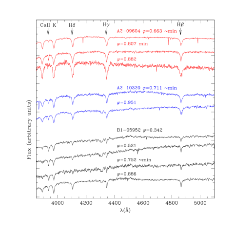
Figure 21: Spectra of the 3 LMC SPC in our sample. For each spectrum we give the corresponding phase along the pulsation cycle. The interval of minimum light is 0.77$<\phi_{min}<0.85$ for star A2-9604, $0.50<\phi_{min}<0.68$ for star A2-10320, and $0.77<\phi_{min}<0.83$ for star B1-5952.

In the derivation of the spectroscopic abundances both the Anomalous Cepheid in $\omega$ Cen (variable #73), and the 3 short period Cepheids in the LMC were analyzed as being normal horizontal branch stars. Indeed, the surface gravity of these supra-HB stars should be similar to that of the RR Lyrae variables, because they are brighter but also likely more massive. We then expect that the metallicity calibration we use, based on normal horizontal branch stars, should be roughly correct also for them. In order to check this assumption in Figure 22 we show the run of the $<H>$ values versus intrinsic (B$-$V)₀ colours for the LMC variables. These colours were derived from the $B,V$ light curves (Di Fabrizio et al. 2004), dereddened according to $E(B-V)_{A}$=0.116 and $E(B-V)_{B}$=0.086 (Clementini et al. 2003a), and correspond to the colour at the phase of each individual spectrum. Only data of stars observed around minimum light are displayed in Figure 22. Different symbols are used for the various types of variables. Two of the RR Lyrae stars (A1-19711 and A2-25301) deviate from the general trend, we suspect that the ephemerides and/or the reddening of these two variables may be wrong. The short period Cepheids (filled symbols in Figure 22) follow the general $<H>-(B-V)_{0}$ relationship defined by the RR Lyrae variables. The SPC spectra closer to minimum light fall on the upper envelope at redder colours of this relation. This suggests that the metallicity calibration we have adopted holds also for the SPCs. However, star B1-05952 falls outside the range defined by the RR Lyrae variables, in a totally extrapolated region of this relation, thus its metal abundance could be slightly overestimated.

Figure 22: Run of $<H>$ with the dereddened $B-V$ colour for the LMC variables observed around minimum light. Different symbols are used for RRab (open circles), RRc (triangles), RRd (squares), and SPC (filled circles) variables. A few of the stars shown in the figure have multiple observations.

The [Fe/H] value we obtain for the $\omega$ Cen candidate Anomalous Cepheid #73 is [Fe/H]$=-1.50\pm 0.12$, in agreement with previous estimates (see Table 6). This star appears to be marginally more metal-rich than the main metal-poor component of $\omega$ Cen at [Fe/H]$\sim-1.6$ (Norris et al. 1996), but definitely metal-poorer than both the secondary metallicity peak at [Fe/H]$\sim-1.2$ (Norris et al. 1996), and the metal-rich peak at [Fe/H]$\sim-0.6$ (Pancino et al. 2002).

For the 3 short period Cepheids in our LMC sample we derive: [Fe/H]=$-1.96\pm 0.16$ for A2-09604, [Fe/H]=$-1.66\pm 0.09$ for A2-10320, and [Fe/H]=$-1.59:\pm 0.03$ for B1-05952, and a corresponding average value of [Fe/H]=$-1.74\pm 0.11$. Both individual and average metallicities of these three variables are well below the average metal abundance of the RR Lyrae stars in our sample ([Fe/H]=$-1.48\pm 0.03$) thus suggesting that these three short period Cepheids are more likely to be Anomalous Cepheids with masses $M\sim 1.3M_{\odot}$ rather than the short period tail of the LMC Classical Cepheids.

It would be important to derive metallicities for more Anomalous Cepheids in different environments. More extensive samples of Anomalous Cepheids with adequate high resolution spectroscopic data would be clearly welcomed.

- (1) Alcock, C. et al. 1996, AJ, 111, 1146
- (2) Blazhko, S. 1907, Astron. Nachr., 175, 325
- (3) Bono, G., Caputo, F., Santolamazza, P., Cassisi, S., & Piersimoni, A. 1997, AJ, 113, 2209
- (4) Bragaglia, A., Gratton, R.G., Carretta, E., Clementini, G., Di Fabrizio, L., & Marconi, M. 2001, AJ, 122, 207
- (5) Brocato, E., Castellani, V., & Ripepi, V. 1994, AJ, 107, 622
- (6) Butler, D., Dickens, R.J., & Epps, E. 1978, ApJ, 225, 148
- (7) Cacciari, C. 1999, in Harmonizing Cosmic Distance Scales in a Post-Hipparcos Era, ed. D. Egret & A. Heck, ASP Conf. ser. 167, 140
- (8) Cacciari, C., & Clementini, G. 2003, in Stellar Candles for the Extragalctic Distance Scale, Lecture Notes in Physics (Berlin: Springer), eds. D. Alloin & W. Gieren, Vol. 635, p. 105 (astro-ph/0301550)
- (9) Carretta, E., Gratton, R.G., Clementini, G., & Fusi Pecci, F. 2000, ApJ, 533, 215
- (10) Caputo, F., Castellani, V., Marconi, M., & Ripepi, V. 2000, MNRAS, 316, 819
- (11) Clement, M.C., Ferance, S., & Simon, N.R. 1993, ApJ, 412, 183
- (12) Clementini, G., Gratton, R., Bragaglia, A., Carretta, E., Di Fabrizio, L., & Maio, M. 2003a, AJ, 125, 1309
- (13) Clementini, G., Held, E.V., Baldacci, L., & Rizzi, L. 2003b, ApJ, 588, 85
- (14) Di Fabrizio, L., Clementini, G., Maio, M., Bragaglia, A., Carretta, E., Gratton, R.G., Montegriffo, P., & Zoccali, M. 2004, A&A, in preparation
- (15) Dolphin, A.E., Saha, A., Claver, J., Skillman, E.D., Cole, A.A., Gallagher, J.S., Tolstoy, E., Dohm-Palmer, R.C., & Mateo, M. 2002, AJ, 123, 3154
- (16) Fernley, J.A, Carney, B.W., Skillen, I., Cacciari, C., & Janes, K. 1998, MNRAS, 293, L61
- (17) Gallart, C., Freedman, W.L., Aparicio, A., Bertelli, G., & Chiosi, C. 1999, AJ, 118, 2245
- (18) Gratton, R.G. 1989, Rome Astron. Obs. Preprint 29
- (19) Gratton, R.G., Tornambè, A., & Ortolani, S., 1986, A&A, 169, 111
- (20) Harris, W.E. 1996, AJ, 112, 1487
- (21) Jurcsik, J. 1995, AcA, 45, 653
- (22) Jurcsik, J. & Kovács, K. 1996, A&A, 312, 111
- (23) Kaluzny, J., Kubiak, M., Szymański, A., Udalski, A., Krzemiński, W., & Mateo, C. 1997, A&AS, 125, 343
- (24) Kovács, K., & Walker, A.R, 2001, A&A, 371, 579
- (25) Marconi, M., Fiorentino, G., & Caputo, F. 2004, A&A, in press (astro-ph/0401332)
- (26) Nemec, J.M., Nemec, A.F.L., & Lutz, T.E. 1994, AJ, 108, 222
- (27) Norris, J.E., Freeman, K.C., & Mighell, K.L. 1996, ApJ, 462, 241
- (28) Pancino, E., Pasquini, L., Hill, V., Ferraro, F.R., & Bellazzini, M. 2002, ApJ, 568, 101
- (29) Pritzl, B. J., Armandroff, T.E., Jacoby, G.H., & Da Costa, G.S. 2002, AJ, 124, 1464
- (30) Preston, G.W. 1959, ApJ, 130, 507
- (31) Rey, S.-C, Lee, Y.-W., Joo, J.-M., Walker, A., & Scott, B. 2000, AJ, 119, 1824
- (32) Rich, M., Corsi, C.E., Bellazzini, M., Federici, L., Cacciari, C. & Fusi Pecci, F. 2001, in IAU Symp. 207, Extragalactic Star Clusters, ed. E.K. Grebel, D. Geisler, & D. Minniti (San Francisco: ASP), p. 140
- (33) Rosenberg, A., Piotto, G.P., Saviane, I., & Aparicio, A. 2000, A&AS, 144, 5
- (34) Sandage, A. 1981a, ApJ, 224, L23
- (35) Sandage, A. 1981b, ApJ, 248, 161
- (36) Sandage, A. 1990, ApJ, 350, 603
- (37) Sandage, A. 1993a, AJ, 106, 703
- (38) Sandage, A. 1993b, AJ, 106, 719
- (39) Sawyer Hogg, H. 1973, Publ. David Dunlap Obs. 3, No. 6
- (40) Smith, H.A., Silbermann, N.A., Baird, S.R., & Graham, J.A. 1992, AJ, 104 1430
- (41) Sturch, C. 1966, ApJ, 143, 774
- (42) Suntzeff, N.B., & Kraft, R.P. 1996, AJ, 111, 1913
- (43) Taribello, E. 2003, Master of Science Thesis, University of Bologna
- (44) Udalski, A., Kubiak, M., & Szymanski, M. 1997, AcA 47, 319
- (45) Walker, A.R. 1992a, ApJL, 390, L81
- (46) Walker, A.R. 1992b, PASP, 104, 1063
- (47) Walker, A.R. 1994, AJ, 108, 555
- (48) Walker, A.R. 1998, AJ, 116, 220
- (49) Zinn, R., & West, M.J. 1984, ApJS, 55, 45