CMB power spectrum estimation using noncircular beams

Abstract

The measurements of the angular power spectrum of the Cosmic Microwave Background (CMB) anisotropy has proved crucial to the emergence of cosmology as a precision science in recent years. In this remarkable data rich period, the limitations to precision now arise from the the inability to account for finer systematic effects in data analysis. The non-circularity of the experimental beam has become progressively important as CMB experiments strive to attain higher angular resolution and sensitivity. We present an analytic framework for studying the leading order effects of a non-circular beam on the CMB power spectrum estimation. We consider a non-circular beam of fixed shape but variable orientation. We compute the bias in the pseudo-$C_{l}$ power spectrum estimator and then construct an unbiased estimator using the bias matrix. The covariance matrix of the unbiased estimator is computed for smooth, non-circular beams. Quantitative results are shown for CMB maps made by a hypothetical experiment with a non-circular beam comparable to our fits to the WMAP beam maps described in the appendix and uses a toy scan strategy. We find that significant effects on CMB power spectrum can arise due to non-circular beam on multipoles comparable to, and beyond, the inverse average beam-width where the pseudo-$C_{l}$ approach may be the method of choice due to computational limitations of analyzing the large datasets from current and near future CMB experiments.

I Introduction

A golden decade of measurements of the cosmic microwave background anisotropy has ushered in an era of precision cosmology. The theory of primary CMB anisotropy is well developed and the past decade has seen a veritable flood of data hu_dod02 ; bon04 . Increasingly sensitive, high resolution, ‘full’ sky measurements from space missions, such as, the ongoing Wilkinson Microwave Anisotropy Probe (WMAP) and, the upcoming Planck surveyor pose a stiff challenge for current analysis techniques to realize the full potential of precise determination of cosmological parameters. As experiments improve in sensitivity, the inadequacy in modeling the observational reality start to limit the returns from these experiments.

A Gaussian model of CMB anisotropy $\Delta T(\mathbf{\hat{q}})$ is completely specified by its angular two-point correlation function. In standard cosmology, CMB anisotropy is expected to be statistically isotropic. In spherical harmonic space, where $\Delta T(\mathbf{\hat{q}})=\sum_{lm}a_{lm}Y_{lm}(\mathbf{\hat{q}})$, this translates to a diagonal $\langle a_{lm}a^{*}_{l^{\prime}m^{\prime}}\rangle=C_{l}\delta_{ll^{\prime}}\delta_{mm^{\prime}}$ where $C_{l}$, the widely used angular power spectrum of CMB anisotropy, is a complete description of a Gaussian CMB anisotropy. Observationally, the angular power spectrum being a simple, robust point statistics is the obvious first target for cosmological observations. Theoretically, the $C_{l}$ are deemed all important since the simplest inflation models predict a Gaussian CMB anisotropy. In this case, the power spectrum provides an economical description of the CMB anisotropy allowing easy comparison to observations.

Accurate estimation of $C_{l}$ is arguably the foremost concern of most CMB experiments. The extensive literature on this topic has been summarized in a recent article efs04 . For Gaussian, statistically isotropic CMB sky, the $C_{l}$ that correspond to covariance that maximize the multivariate Gaussian PDF of the temperature map, $\Delta T(\mathbf{\hat{q}})$ is the Maximum Likelihood (ML) solution. Different ML estimators have been proposed and implemented on CMB data of small and modest size gor94 ; gor_hin94 ; gor96 ; gor97 ; max97 ; bjk98 . While it is desirable to use optimal estimators of $C_{l}$ that obtain (or iterate toward) the ML solution for the given data, these methods usually are limited by the computational expense of matrix inversion that scales as $N_{d}^{3}$ with data size $N_{d}$ bor99 ; bon99 . Various strategies for speeding up ML estimation have been proposed, such as, exploiting the symmetries of the scan strategy oh_sper99 , using hierarchical decomposition dor_knox01 , iterative multi-grid method pen03 , etc. Variants employing linear combinations of $\Delta T(\mathbf{\hat{q}})$ such as $a_{lm}$ on set of rings in the sky can alleviate the computational demands in special cases harm02 ; wan_han03 . Other promising exact power estimation methods have been recently proposed wan_lar03 ; wan04 ; jew02 .

However there also exist computationally rapid, sub-optimal estimators of $C_{l}$. Exploiting the fast spherical harmonic transform ($\sim N_{d}^{3/2}$), it is possible to estimate the angular power spectrum $C_{l}=\langle|a_{lm}|^{2}\rangle/(2l+1)$ rapidly yu_peeb69 ; peeb73 . This is commonly referred to as the pseudo-$C_{l}$ method wan_hiv03 . (Analogous approach employing fast estimation of the correlation function $C(\mathbf{\hat{q}}\cdot\mathbf{\hat{q}^{\prime}})$ have also been explored szap01 ; szap_prun01 .) It has been recently argued that the need for optimal estimators may have been over-emphasized since they are computationally prohibitive at large $l$ . Sub-optimal estimators are computationally tractable and tend to be nearly optimal in the relevant high $l$ regime. Moreover, already the data size of the current sensitive, high resolution, ‘full sky’ CMB experiments such as WMAP have compelled the use of sub-optimal pseudo-$C_{l}$ related methods Bennett:2003 ; hin_wmap03 . On the other hand, optimal ML estimators can readily incorporate and account for various systematic effects, such as non-uniform sky coverage, noise correlations and beam asymmetries.

In the years after the COBE-DMR observations cobedmr92 , more sensitive measurements at higher resolution but with limited sky coverage were made by a number of experiments . The effect of incomplete (more generally, non uniform) sky coverage on the sampling statistics of $C_{l}$ was the dominant concern of these experiments such as the ground based experiment TOCO toco , DASI dasi , CBI cbi , ACBAR acbar , and balloon based experiments BOOMERang boom , MAXIMA maxima ; lee01 and Archeops ben03 . Comprehensive analyzes have been carried out to tackle this problem. For example, the basic semi-analytic framework developed wan_hiv03 was subsequently implemented as fast, efficient scheme for the analysis of the BOOMERang experiment master . While the non-uniform sky coverage has been addressed in the pseudo-$C_{l}$ method, the other effects remain to be incorporated.

In this paper, we initiate a similar line of research to address a more contemporary issue that has gained relative importance in the post WMAP Bennett:2003 (and pre-Planck) era of CMB anisotropy measurement with ‘full’ sky coverage. It has been usual in CMB data analysis to assume the experimental beam response to be circularly symmetric around the pointing direction. However, any real beam response function has deviations from circular symmetry. Even the main lobe of the beam response of experiments are generically non-circular (non-axisymmetric) since detectors have to be placed off-axis on the focal plane. (Side lobes and stray light contamination add to the breakdown of this assumption). For high sensitive experiments, the systematic errors arising from the beam non-circularity become progressively more important. Recent CMB experiments such as ARCHEOPS, MAXIMA, WMAP have significantly non-circular beams. Future experiments like the Planck Surveyor are expected to be even more seriously affected by non-circular beams.

Dropping the circular beam assumption leads to major complications at every stage of the data analysis pipeline. The extent to which the non-circularity affects the step of going from the time-stream data to sky map is very sensitive to the scan-strategy. The beam now has an orientation with respect to the scan path that can potentially vary along the path. This implies that the beam function is inherently time dependent and difficult to deconvolve. Even after a sky map is made, the non-circularity of the effective beam affects the estimation of the angular power spectrum, $C_{l}$, by coupling the $l$ modes, typically, on scales beyond the inverse angular beam-width.

Barring few exceptions (eg., wan_gor01 ), the non-circularity of beam patterns in CMB experiments has been addressed in limited context. When it has not been totally ignored, one has measured with numerical simulations the biasing effect on the power spectrum of CMB anisotropies of neglecting the non-circularity of the beams in the data analysis chain (see e.g., MAXIMA lee01 ; whu01 , Archeops ben03 ; asym_04 ). This approach only deals with the diagonal part of the matrix relating the observed power spectrum to the underlying power spectrum, so does not fully describe the effect of the beam complexity on the CMB statistics. An integrated approach to account for the systematic effect of a non-circular beam has not yet been developed.

In this initial work we skip over the issues related to map making and focus on the CMB power spectrum estimation from a CMB sky map made with an effective beam that is non-circular. Mild deviations from circularity can be addressed by a perturbation approach  TR:2001 ; fos02 . Besides providing an elegant analytic formalism, the approach has lead to rapid methods for computing the window functions for CMB experiments pyV . In this work the effect of beam non-circularity on the estimation of CMB power spectrum is studied analytically using this perturbation approach.

We present a brief primer on the connection between CMB power spectrum and the experimental window functions in section II. The section is designed to keep the paper self-contained and also serves to set the notation for the rest of the paper. In section II.2, we briefly review the perturbation approach for computing the the window functions for CMB experiments with non-circular beam TR:2001 and also define the elliptical Gaussian beam and its spherical transform. The bias matrix accounting for the non-circularity of the beam for the pseudo-$C_{l}$ estimator of CMB anisotropy is derived and discussed in section III. The error-covariance for the unbiased estimator is derived in section III. We conclude with a discussion of the results in section IV. An interesting exercise of fitting the WMAP beam maps with an elliptical Gaussian beam profile is presented in an appendix A. Details of the steps leading to our analytical results are given in Appendix B.

II Window functions of CMB experiments: a brief primer

Conventionally, the CMB temperature, $\Delta T(\mathbf{\hat{q}})$, is expressed as a function of angular position, $\mathbf{\hat{q}}\equiv(\theta,\phi)$, on the sky via the spherical harmonic decomposition,

$$\Delta T(\mathbf{\hat{q}})=\sum^{\infty}_{l=0}\sum^{l}_{m=-l}a_{lm}Y_{lm}(\mathbf{\hat{q}})\,.$$ (1)

In an idealized noise free, CMB anisotropy sky map $\Delta T(\mathbf{\hat{q}})$ made with infinitely high resolution, the angular power spectrum is given by

$$C_{l}\ \equiv\ \frac{1}{2l+1}\sum_{m=-l}^{l}\langle|a_{lm}|^{2}\rangle,$$ (2)

where

$$a_{lm}\ \equiv\ \int d\Omega_{\mathbf{\hat{q}}}\,Y_{lm}^{*}(\mathbf{\hat{q}})\,\Delta T(\mathbf{\hat{q}})$$ (3)

are the spherical harmonic transforms of the temperature deviation field $\Delta T(\mathbf{\hat{q}})$. We introduce the scaled power spectrum $\mathcal{C}_{l}\equiv(l(l+1)/2\pi)C_{l}$, that measures the power per logarithmic interval of angular scale, $l$. Eliminating $a_{lm}$, we may write,

$$\mathcal{C}_{l}\ =\ \frac{l(l+1)}{8\pi^{2}}\int d\Omega_{\mathbf{\hat{q}}_{1}}\int d\Omega_{\mathbf{\hat{q}}_{2}}\langle\Delta T(\mathbf{\hat{q}}_{1})\Delta T(\mathbf{\hat{q}}_{2})\rangle P_{l}(\mathbf{\hat{q}}_{1}\cdot\mathbf{\hat{q}}_{2}),$$ (4)

where we have made use of the expansion of Legendre Polynomials

$$P_{l}(\mathbf{\hat{q}}_{1}\cdot\mathbf{\hat{q}}_{2})\ =\ \frac{4\pi}{2l+1}\sum_{m=-l}^{l}Y_{lm}^{*}(\mathbf{\hat{q}}_{1})Y_{lm}(\mathbf{\hat{q}}_{2}).$$ (5)

If we assume the isotropy of the CMB sky, $\langle\Delta T(\mathbf{\hat{q}}_{1})\Delta T(\mathbf{\hat{q}}_{2})\rangle$ should depend only on $\mathbf{\hat{q}}_{1}\cdot\mathbf{\hat{q}}_{2}$. Therefore, we can use Legendre expansion to show that,

$$\langle\Delta T(\mathbf{\hat{q}}_{1})\Delta T(\mathbf{\hat{q}}_{2})\rangle\ =\ \sum_{l=0}^{\infty}\frac{2l+1}{2l(l+1)}\,\mathcal{C}_{l}\,P_{l}(\mathbf{\hat{q}}_{1}\cdot\mathbf{\hat{q}}_{2}).$$ (6)

All CMB anisotropy experiments measure differences in CMB temperature at different locations on the sky. A step of map-making is required to derive the above temperature anisotropy map at each point on the sky. Since this is a linear operation, the correlation function of the measured quantity for a given scanning or modulation strategy can always be expressed as linear sum of ‘elementary’ correlations of the temperature given in eq. (6).

Typically, a CMB anisotropy experiment probes a range of angular scales characterized by a window function $W_{l}(\mathbf{\hat{q}},\mathbf{\hat{q}}^{\prime})$. The window depends both on the scanning strategy as well as the angular resolution and response of the experiment. However, it is neater to logically separate these two effects by expressing the window $W_{l}(\mathbf{\hat{q}},\mathbf{\hat{q}}^{\prime})$ as a sum of ‘elementary’ window function of the CMB anisotropy at each point of the map TR:2001 . In this work, we only deal with these elementary window functions. For a given scanning/modulation strategy, our results can be readily generalized using the representation of the window function as sum over elementary window functions (see, e.g., TR:2001 ; pyV ). Although the quantitative results we present in this paper refer to a scan strategy where each pixel is visited by the beam only once, this is not a limitation of our approach. If pixels are multiply visited by the beam with different orientations, the correlation function still can be expressed as a sum over appropriate elementary window functions for which all the results we describe in this paper hold.

II.1 Window function for circular beams

Due to finite resolution of the instruments, the ‘measured’ temperature difference $\widetilde{\Delta T}(\mathbf{\hat{q}})$ along the direction $\mathbf{\hat{q}}$ in response to the CMB anisotropy signal $\Delta T(\mathbf{\hat{q}}^{\prime})$ is given by

$$\widetilde{\Delta T}(\mathbf{\hat{q}})\ =\ \int d\Omega_{\mathbf{\hat{q}}^{\prime}}\,B(\mathbf{\hat{q}},\mathbf{\hat{q}}^{\prime})\,\Delta T(\mathbf{\hat{q}}^{\prime})$$ (7)

where the experimental “Beam” response function $B(\mathbf{\hat{q}},\mathbf{\hat{q}}^{\prime})$ describes the sensitivity of the measuring instrument at different angles around the pointing direction. There is an additional contribution from instrumental noise denoted by $n(\mathbf{\hat{q}})$ which we shall introduce later into our final results.

The two point correlation function for a statistical isotropic CMB anisotropy signal is

$$C(\mathbf{\hat{q}},\mathbf{\hat{q}}^{\prime})=\langle\widetilde{\Delta T}(\mathbf{\hat{q}})\widetilde{\Delta T}(\mathbf{\hat{q}^{\prime}})\rangle=\sum^{\infty}_{l=0}{(2l+1)\over 4\pi}\,C_{l}\,\,W_{l}(\mathbf{\hat{q}},\,\mathbf{\hat{q}}^{\prime})\,,$$ (8)

where $C_{l}$ is the angular spectrum of CMB anisotropy signal and the window function

$$W_{l}(\mathbf{\hat{q}}_{1},\mathbf{\hat{q}}_{2})\ \equiv\ \int d\Omega_{\mathbf{\hat{q}}}\int d\Omega_{\mathbf{\hat{q}^{\prime}}}\,B(\mathbf{\hat{q}}_{1},\mathbf{\hat{q}})B(\mathbf{\hat{q}}_{2},\mathbf{\hat{q}^{\prime}})P_{l}(\mathbf{\hat{q}}\cdot\mathbf{\hat{q}^{\prime}}),$$ (9)

encodes the effect of finite resolution through the beam function.

For some experiments, the beam function may be assumed to be circularly symmetric about the pointing direction, i.e., $B(\mathbf{\hat{q}},\mathbf{\hat{q}}^{\prime})\equiv B(\mathbf{\hat{q}}\cdot\mathbf{\hat{q}}^{\prime})$ without significantly affecting the results of the analysis. In any case, this assumption allows a great simplification since the beam function can then be represented by an expansion in Legendre polynomials as

$$B(\mathbf{\hat{q}}\cdot\mathbf{\hat{q}^{\prime}})\ =\ \frac{1}{4\pi}\,\sum_{l=0}^{\infty}\,(2l+1)\,B_{l}\,P_{l}(\mathbf{\hat{q}}\cdot\mathbf{\hat{q}^{\prime}}).$$ (10)

Consequently, it is straightforward to derive the well known simple expression

$$W_{l}(\mathbf{\hat{q}},\,\mathbf{\hat{q}^{\prime}})\ =\ B^{2}_{l}\,P_{l}(\mathbf{\hat{q}}\cdot\mathbf{\hat{q}^{\prime}})\,,$$ (11)

for a circularly symmetric beam function.

II.2 Window function for non-circular beams

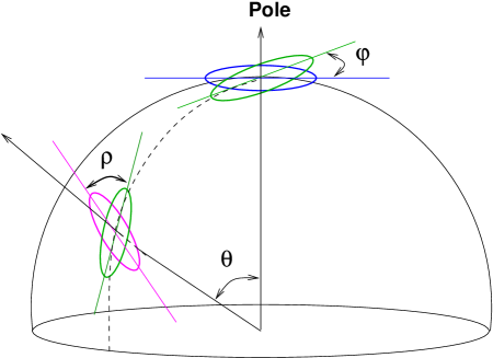
Figure 1: The figure illustrates that a beam pointed in an arbitrary direction $\mathbf{\hat{q}}=(\theta,\phi)$, with an orientation given by the angle $\rho(\mathbf{\hat{q}})$ can always be rotated to point along $\mathbf{\hat{z}}$ oriented with $\rho(\mathbf{\hat{z}})=0$. The Euler angles of this rotation are clearly seen to be $(\theta,\phi,\rho)$. Consequently, the beam transforms are related through Wigner rotation matrices corresponding to the same rotation.

While some experiments may have circularly symmetric beam functions, most experimental beams are non-circular to some extent. The effect of non-circularity of the beam has become progressively more relevant for experiments with higher sensitivity and angular resolution. The most general beam response function can be represented as

$$B(\mathbf{\hat{z}},\mathbf{\hat{q}})\ =\ \sum_{l=0}^{\infty}\sum_{m=-l}^{l}b_{lm}(\mathbf{\hat{z}})\,Y_{lm}(\mathbf{\hat{q}})$$ (12)

by a spherical harmonic expansion when pointing along $\mathbf{\hat{z}}$ axis (“North pole” in some given astronomical coordinate system). In case of circularly symmetric beams, the real coefficients $B_{l}=\sqrt{4\pi/(2l+1)}b_{l0}$.

For mild deviations, the non-circularity of the beams can be parameterized by a set of small quantities $\beta_{lm}\equiv b_{lm}/b_{l0}$ – the Beam Distortion Parameters (BDP). The smoothness of the beam response implies that at any multipole $l$, the coefficients $\beta_{lm}$ decrease sufficiently rapidly with increasing $|m|$. In addition, for the rest of paper we assume that the beam function has reflection symmetry about two orthogonal axes on the (locally flat) beam plane, which ensures that the coefficients $b_{lm}(\mathbf{\hat{z}})$ are real and zero for odd values of $m$. An example of a non-circular beam with such symmetries is the elliptical Gaussian beam. A brief mathematical description of such beams can be found later in this section. In order to verify our analytical results, we have used the elliptical Gaussian beam as a model of non-circular beam. However, our analytic results would apply to a general form of non-circular beam (as long as $\beta_{l1}$ is zero or sub-dominant to $\beta_{l2}$).

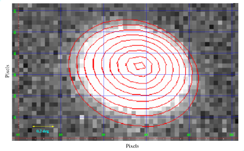
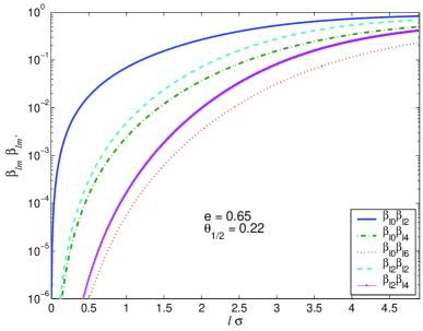
Figure 2: The left panel shows the WMAP Q1 (A side) beam map overlaid with IRAF fitted ellipses over iso-intensity contours. More details are in Appendix A. On the right panel, we plot the product of beam distortion parameters for the elliptic Gaussian fit to the WMAP-Q1 beam versus multipole corresponding to the different order of the perturbation expansion of a window function for a non-circular beam. Note that the effect kicks in at $l\bar{\sigma}\sim 1$.

In order to find an expression for window function in terms of the $\beta_{lm}$ and $B_{l}$, we follow the approach in TR:2001 . The beam transforms for an arbitrary pointing direction $\mathbf{\hat{q}}$ may be expressed as,

$$b_{lm}(\mathbf{\hat{q}})\ =\ \sum_{m^{\prime}=-l}^{l}b_{lm^{\prime}}(\mathbf{\hat{z}})D_{mm^{\prime}}^{l}(\mathbf{\hat{q}},\rho(\mathbf{\hat{q}})),$$ (13)

where $D_{mm^{\prime}}^{l}(\mathbf{\hat{q}},\rho)\equiv D_{mm^{\prime}}^{l}(\phi,\theta,\rho)$ are the Wigner-$D$ functions given in terms of the Euler angles describing the rotation that carries the pointing direction $\mathbf{\hat{q}}$ to $\mathbf{\hat{z}}$-axis, as illustrated in Figure 1. The third angle $\rho(\mathbf{\hat{q}})$ measures the angle by which the beam has rotated about the new pointing direction, when the pointing direction moves from $\mathbf{\hat{z}}$ to $\mathbf{\hat{q}}$ . Inserting the spherical transform of the beam in eq. (13) into eq. (9) we can write the window function as

$$W_{l}(\mathbf{\hat{q}}_{1},\mathbf{\hat{q}}_{2}) = \frac{4\pi}{2l+1}\sum_{m=-l}^{l}b_{lm}^{*}(\mathbf{\hat{q}}_{1})b_{lm}(\mathbf{\hat{q}}_{2})$$ (14)

$$= B_{l}^{2}\sum_{m_{1}=-l}^{l}\sum_{m_{2}=-l}^{l}\beta_{lm_{1}}^{*}\beta_{lm_{2}}\sum_{m=-l}^{l}D_{mm_{1}}^{l*}(\mathbf{\hat{q}}_{1},\rho(\mathbf{\hat{q}}_{1}))D_{mm_{2}}^{l}(\mathbf{\hat{q}}_{2},\rho(\mathbf{\hat{q}}_{2}))$$ (15)

solely in terms of the circular component of the beam function $B_{l}$ and non-circular parts encoded in the BDP’s, $\beta_{lm}$. As pointed out in  TR:2001 , the window function expressed in the form of eq. (15) has an obvious expansion in perturbation series in $\beta_{lm}$ retaining only the lowest values of $|m_{1}|$ and $|m_{2}|$. In this paper, we adopt this perturbation approach to evaluate the leading order correction to power spectrum estimation arising due to mild deviations of the beam from circular symmetry.

For numerical evaluation it is advantageous to use the summation formula of Wigner-$D$ to combine the product of the two Wigner-$D$ functions in eq. (15) into a single one as  TR:2001

$$W_{l}(\mathbf{\hat{q}}_{1},\mathbf{\hat{q}}_{2})={4\pi\over 2l+1}\sum^{l}_{m^{\prime}=-l}\,\sum^{l}_{m^{\prime\prime}=-l}\left[b_{lm^{\prime}}(\mathbf{\hat{z}})\right]^{*}b_{lm^{\prime\prime}}(\mathbf{\hat{z}})D^{l}_{m^{\prime}m^{\prime\prime}}(\alpha-\rho_{1},\,\gamma,\,\beta+\rho_{2}),$$ (16)

where

$${\rm cos}\gamma = \mathbf{\hat{q}}_{1}\cdot\mathbf{\hat{q}}_{2}$$

$${\rm cot}\alpha = -{\rm cos}\theta_{1}\,{\rm cot}(\phi_{1}-\phi_{2})+{\rm sin}\theta_{1}\,{\rm cot}\theta_{2}\,{\rm csc}(\phi_{1}-\phi_{2})$$ (17)

$${\rm cot}\beta = -{\rm cos}\theta_{2}\,{\rm cot}(\phi_{1}-\phi_{2})+{\rm cot}\theta_{1}\,{\rm sin}\theta_{2}\,{\rm csc}(\phi_{1}-\phi_{2}).$$

For large values of $l$ it is computationally expensive to evaluate the entire $m^{\prime}$ and $m^{\prime\prime}$ sum in eq. (16). However, for a smooth, mildly non-circular beam function, restricting the summation to a few low values of $m^{\prime}$ and $m^{\prime\prime}$ results in a good approximation. The leading order terms in the perturbation TR:2001

$$W_{l}(\mathbf{\hat{q}}_{1},\,\mathbf{\hat{q}}_{2}) = {4\pi\over 2l+1}\bigg{[}\left[b_{l0}(\mathbf{\hat{z}})\right]^{2}d^{l}_{00}(\gamma)+2b_{l0}(\mathbf{\hat{z}})b_{l2}(\mathbf{\hat{z}})\left\{{\rm cos}(2(\alpha-\rho_{1}))+{\rm cos}(2(\beta+\rho_{2}))\right\}d^{l}_{02}(\gamma)$$ (18)

$$+2\left[b_{l2}(\mathbf{\hat{z}})\right]^{2}\left[{\rm cos}(2(\alpha+\beta+\rho_{2}-\rho_{1}))d^{l}_{22}(\gamma)+(-1)^{-l}{\rm cos}(2(\alpha-\beta-\rho_{1}-\rho_{2})))d^{l}_{22}(\pi-\gamma)\right]$$

$$+2b_{l0}(\mathbf{\hat{z}})b_{l4}(\mathbf{\hat{z}})\left\{{\rm cos}(4(\alpha-\rho_{1}))+{\rm cos}(4(\beta+\rho_{2}))\right\}d^{l}_{04}(\gamma)+\cdots\bigg{]}.$$

can be readily evaluated using recurrence relations similar to that of Legendre function. In the above we have restricted to the common situation of beam functions with reflection symmetry ($\beta_{lm}$ are real and $\beta_{lm}=0$ for odd $m$) such as the elliptic Gaussian beam described next.

An elliptic Gaussian beam profile, pointed along the $\mathbf{\hat{z}}$-axis is expressed in terms of the spherical polar coordinates about the pointing direction as follows TR:2001

$$B(\mathbf{\hat{z}},\mathbf{\hat{q}})\ =\ \frac{1}{2\pi\sigma_{1}\sigma_{2}}\exp\left[-\frac{\theta^{2}}{2\sigma^{2}(\phi)}\right],$$ (19)

where the “beam-width” $\sigma(\phi)\ \equiv\ [\sigma_{1}^{2}/(1+\epsilon\sin^{2}\phi)]^{1/2}$ and the “non-circularity parameter” $\epsilon\ \equiv\ (\sigma_{1}^{2}/\sigma_{2}^{2}-1)$ are given in terms of $\sigma_{1}$ and $\sigma_{2}$ – the Gaussian widths along the semi-major and semi-minor axis, respectively. However, we characterize an elliptical beam using two different parameters: eccentricity $e\equiv\sqrt{1-\sigma_{2}^{2}/\sigma_{1}^{2}}$ and the size parameter $\theta_{1/2}$, the FWHM of a circular beam of equal “area”.

For elliptical Gaussian beams the spherical harmonic transform is available in the closed analytical form

$$b_{lm}\ =\ \left[\frac{2l+1}{4\pi}\,\frac{(l+m)!}{(l-m)!}\right]^{\frac{1}{2}}(l+1/2)^{-m}I_{m/2}\left[\frac{(l+1/2)^{2}\sigma_{1}^{2}e^{2}}{4}\right]\,\exp\left[-\frac{(l+1/2)^{2}\sigma_{1}^{2}}{2}\left\{1-\frac{e^{2}}{2}\right\}\right]\,,$$ (20)

where $I_{\nu}(x)$ is the modified Bessel function TR:2001 ; Challinor . Note, in the above equation we have used eccentricity $e$ instead of the non-circularity parameter $\epsilon=e^{2}/(1-e^{2})$ used in TR:2001 . (Please see Table LABEL:tab:2 for the various definitions and characterizations of elliptical beams.)

Table 1: In literature, the elliptical beams have been described by several parameters which can all be expressed in terms of the Gaussian widths along the semi-major ($\sigma_{1}$) and the semi-minor ($\sigma_{2}$) axes of the ellipse. We have used these parameters at several places in the paper.

Parameter	Symbol	Expression
Eccentricity	$e$	$\sqrt{1-\frac{\sigma_{2}^{2}}{\sigma_{1}^{2}}}$
Non-Circularity Parameter	$\epsilon$	$\frac{\sigma_{1}^{2}}{\sigma_{2}^{2}}-1$
Ellipticity	$\bar{\epsilon}$	$1-\frac{\sigma_{2}}{\sigma_{1}}$

Fig 2 shows one of the WMAP beams as an example of a distinctly non-circular beam (see iso-contours in the left panel) that can be efficiently handled by the leading order term in the perturbation approach (see the right panel). Details of the exercise of fitting elliptical Gaussian beam profile to the WMAP beam maps is given in appendix A.

III Bias Matrix

Given the observed temperature fluctuations $\widetilde{\Delta T}(\mathbf{\hat{q}})$, a naive estimator for the angular power spectrum based on eq. (2) is given by

$$\widetilde{\mathcal{C}}_{l}\equiv\ \frac{l(l+1)}{2\pi}\frac{1}{2l+1}\sum_{m=-l}^{l}|\tilde{a}_{lm}|^{2},$$ (21)

where

$$\tilde{a}_{lm}\ \equiv\ \int d\Omega_{\mathbf{\hat{q}}}\,Y_{lm}^{*}(\mathbf{\hat{q}})\,\widetilde{\Delta T}(\mathbf{\hat{q}})\,w(\mathbf{\hat{q}})$$ (22)

are the coefficients of the spherical harmonic transform of the CMB anisotropy map yu_peeb69 ; peeb73 . The weight function $w(\mathbf{\hat{q}})$ accounts for non-uniform/incomplete sky coverage and also provides a handle to weigh the data ‘optimally’. Without the inconsequential $l(l+1)$ scaling, this naive estimator is referred to as the pseudo-$C_{l}$ in recent literature wan_hiv03 . The ‘pseudo’ refers to fact that the estimated $C_{l}$ is biased. Moreover, this is a sub-optimal estimator of the power spectrum. This naive power spectrum estimate has to be corrected for observational effects such as the instrumental noise contribution, beam resolution, incomplete/non-uniform sky coverage. Nevertheless, the pseudo-$C_{l}$ method is a computationally fast and economical approach and is currently a method of choice for the recent large CMB anisotropy datasets (at least for large $l$ within the hybrid schemes efs04 ).

Faced with the computational challenges of large data sets, an approach that has been adopted is to compute the pseudo-$C_{l}$’s from the CMB observations and then correct for the observational effects. The true $C_{l}$ spectrum is linearly related

$$\langle\tilde{\mathcal{C}}_{l}\rangle=\sum_{{l^{\prime}}}A_{l{l^{\prime}}}\,{\mathcal{C}}_{l^{\prime}}$$ (23)

to the pseudo-$C_{l}$ through a bias matrix $A_{l{l^{\prime}}}$. Similar bias matrices arising due to the effect of non-uniform sky coverage, instrumental noise have been studied wan_hiv03 ; master . In this paper, we compute the $A_{l{l^{\prime}}}$ for non-circular beam and give explicit analytical results for the leading order terms for non rotating beams.

The pseudo-$C_{l}$ estimator in eq. (21) can be expressed as

$$\widetilde{\mathcal{C}}_{l}\ \equiv\ \frac{l(l+1)}{8\pi^{2}}\int d\Omega_{\mathbf{\hat{q}}_{1}}\int d\Omega_{\mathbf{\hat{q}}_{2}}\,w(\mathbf{\hat{q}}_{1})w(\mathbf{\hat{q}}_{2})\,\widetilde{\Delta T}(\mathbf{\hat{q}}_{1})\widetilde{\Delta T}(\mathbf{\hat{q}}_{2})P_{l}(\mathbf{\hat{q}}_{1}\cdot\mathbf{\hat{q}}_{2}).$$ (24)

The ensemble expectation value of the pseudo-$C_{l}$ power spectrum estimator is

$$\langle\widetilde{\mathcal{C}}_{l}\rangle = \frac{l(l+1)}{8\pi^{2}}\int d\Omega_{\mathbf{\hat{q}}_{1}}\int d\Omega_{\mathbf{\hat{q}}_{2}}\,w(\mathbf{\hat{q}}_{1})w(\mathbf{\hat{q}}_{2})\,\times$$ (25)

$$\sum_{l^{\prime}}\frac{2{l^{\prime}}+1}{2{l^{\prime}}({l^{\prime}}+1)}\mathcal{C}_{l^{\prime}}P_{l}(\mathbf{\hat{q}}_{1}\cdot\mathbf{\hat{q}}_{2})\int d\Omega_{\mathbf{\hat{q}}}\int d\Omega_{\mathbf{\hat{q}^{\prime}}}\,B(\mathbf{\hat{q}}_{1},\mathbf{\hat{q}})B(\mathbf{\hat{q}}_{2},\mathbf{\hat{q}^{\prime}})P_{l^{\prime}}(\mathbf{\hat{q}}\cdot\mathbf{\hat{q}^{\prime}}).$$

Recalling the definition of a window function in eq. (9), the most general form of the bias matrix

$$A_{l{l^{\prime}}}\ =\ \frac{2{l^{\prime}}+1}{16\pi^{2}}\frac{l(l+1)}{{l^{\prime}}({l^{\prime}}+1)}\int d\Omega_{\mathbf{\hat{q}}_{1}}\int d\Omega_{\mathbf{\hat{q}}_{2}}\,w(\mathbf{\hat{q}}_{1})w(\mathbf{\hat{q}}_{2})\,P_{l}(\mathbf{\hat{q}}_{1}\cdot\mathbf{\hat{q}}_{2})W_{l^{\prime}}(\mathbf{\hat{q}}_{1},\mathbf{\hat{q}}_{2}).$$ (26)

Using the expression for the window function for a non circular beam in eq. (15) the bias matrix can be written as

$$A_{ll^{\prime}}=\ \frac{B_{l^{\prime}}^{2}}{4\pi}\frac{(2l^{\prime}+1)}{(2l+1)}\frac{l(l+1)}{l^{\prime}(l^{\prime}+1)}\times\sum_{n=-l}^{l}\sum_{m=-{l^{\prime}}}^{{l^{\prime}}}\left|\sum_{m^{\prime}=-{l^{\prime}}}^{{l^{\prime}}}\beta_{{l^{\prime}}m^{\prime}}\int d\Omega_{\mathbf{\hat{q}}}\,Y_{ln}^{*}(\mathbf{\hat{q}})\,D_{mm^{\prime}}^{{l^{\prime}}}(\mathbf{\hat{q}},\rho(\mathbf{\hat{q}}))\,w(\mathbf{\hat{q}})\right|^{2}.$$ (27)

The above expressions in eq. (26) and eq. (27) are valid for a completely general non-circular beam with an arbitrary orientation at each point. The scan pattern of the CMB experiment and relative orientation of the beam along it is encoded in the function $\rho(\mathbf{\hat{q}})$. The weight $w(\mathbf{\hat{q}})$ can account for non-uniform sky coverage. Analytical progress can be made when $w(\mathbf{\hat{q}})\equiv w(\theta)$ and $\rho(\mathbf{\hat{q}})=\rho(\theta)$ are fixed along a given declination, but we do not discuss further it here. When the beam transform, weight function and the scan pattern are specified, the bias matrix can be evaluated numerically using eq. (27). However, for mild deviations from circularity, the above expression also points to a perturbation expansion in the small beam distortion parameters, $\beta_{lm}$.

For obtaining fully analytical results, we set the weight function $w(\mathbf{\hat{q}})=1$, corresponding to a full, uniform sky coverage and also limit attention to scans with ‘non-rotating’ beams where $\rho(\mathbf{\hat{q}})=0$. This is presented in the next subsections

III.1 Circular Symmetric Beam

We first consider eq. (27) for the simpler and well studied case of a circular beam. For clarity of presentation, we limit our discussion full, uniform sky coverage ($w(\mathbf{\hat{q}})=1$). Results for non-uniform coverage with a circular beam are available in the literature wan_hiv03 ; master ; efs04 .

Using the expression for the window function for circular beam eq. (11) into the expression for the bias in eq. (26) we recover

$$A_{l{l^{\prime}}}\ =\ B_{l}^{2}\,\delta_{l{l^{\prime}}}\ \ \Rightarrow\ \langle\widetilde{\mathcal{C}}_{l}\rangle\ =\ B_{l}^{2}\,\mathcal{C}_{l}.$$ (28)

For a full sky measurement with a circular beam, the bias matrix is diagonal implying that there is no mixing of power between different multipoles. The true expectation value of the power spectrum can be obtained by dividing the pseudo-$C_{l}$ estimator by the isotropic beam transform $B_{l}^{2}$.

Next we account for the noise contribution and recover the well known result for a full sky observation. The pixel noise $n(\mathbf{\hat{q}})$ adds to the observed temperature, so that the resultant observed temperature

$$\widetilde{\Delta T}^{\prime}(\mathbf{\hat{q}})\ =\ \widetilde{\Delta T}(\mathbf{\hat{q}})+n(\mathbf{\hat{q}})$$ (29)

and we can readily obtain

$$\langle\widetilde{\mathcal{C}}_{l}^{\prime}\rangle\ =\ \langle\widetilde{\mathcal{C}}_{l}\rangle\ +\ \mathcal{C}_{l}^{N}\ =\ B_{l}^{2}\,\mathcal{C}_{l}\ +\ \mathcal{C}_{l}^{N},$$ (30)

where $\mathcal{C}_{l}^{N}$ is the angular power spectrum of the noise $n(\mathbf{\hat{q}})$ is a well determined quantity. The unbiased estimator for $\mathcal{C}_{l}$ obtained is

$$\widetilde{\mathcal{C}}_{l}^{UB}\ =\ B_{l}^{-2}\,\left(\widetilde{\mathcal{C}}_{l}^{\prime}\ -\ \mathcal{C}_{l}^{N}\right).$$ (31)

III.2 Non-circular Beam

We obtain analytic results for the bias matrix for a full sky observation ($w(\mathbf{\hat{q}})=1$) with a non-circular beam that ‘does not rotate’. The phrase “non-rotating” means that the orientation of the non-circular beam does not rotate about its axis (the pointing direction) while the pointing direction scans the sky implying that

$$\rho(\mathbf{\hat{q}})\ =\ 0.$$ (32)

For non-rotating beam, the calculation of the bias is completely analytically tractable. The integral in the expression for the bias in eq. (27) is given by

$$\int Y_{ln}^{*}(\mathbf{\hat{q}})\,D_{mm^{\prime}}^{{l^{\prime}}}(\mathbf{\hat{q}},0)\,d\Omega_{\mathbf{\hat{q}}}\ =\ \sqrt{(2l+1)\pi}\ I_{mm^{\prime}}^{l{l^{\prime}}}\,\delta_{mn},$$ (33)

where

$$I_{mm^{\prime}}^{l{l^{\prime}}}\ \equiv\ \int_{-1}^{1}d_{m0}^{l}(\theta)\,d_{mm^{\prime}}^{{l^{\prime}}}(\theta)\,d\cos\theta,$$ (34)

and $d_{mm^{\prime}}^{l}(\theta)$ are Wigner-$d$ functions related to Wigner-$D$ functions

$$D_{mm^{\prime}}^{l}(\mathbf{\hat{q}},\rho)\ =\ e^{-im\phi}\,d_{mm^{\prime}}^{l}(\theta)e^{-im^{\prime}\rho}.$$ (35)

The analytic simplicity arises from the fact that for $\rho(\mathbf{\hat{q}})=0$, the Wigner-$D$ function reduces to spherical harmonic function

$$Y_{lm}(\mathbf{\hat{q}})\ =\ \sqrt{\frac{2l+1}{4\pi}}\,D_{m0}^{l}(\mathbf{\hat{q}},0)\,.$$ (36)

In deriving the above have used the orthogonality of the phases $\int_{0}^{2\pi}\,e^{-i(m-n)\phi}d\phi\ =\ 2\pi\delta_{mn}$.

Substituting the expression for the integral eq. (33) into the expression for the bias in eq. (27), we obtain

$$A_{l{l^{\prime}}}\ =\ B_{l^{\prime}}^{2}\left(\frac{2{l^{\prime}}+1}{4}\right)\frac{l(l+1)}{{l^{\prime}}({l^{\prime}}+1)}\sum_{m=-L}^{L}\left|\sum_{m^{\prime}=-{l^{\prime}}}^{{l^{\prime}}}\beta_{{l^{\prime}}m^{\prime}}\ I_{mm^{\prime}}^{l{l^{\prime}}}\right|^{2},$$ (37)

where $L\equiv{\rm min}\{l,{l^{\prime}}\}$ is the smaller between $l$ and ${l^{\prime}}$.

Further analytical progress is possible for smooth beam with mild deviations from circular symmetry through a perturbation in terms of the small beam distortion parameters, $\beta_{lm}$. We calculate the exact analytic expression for the leading order effect. Assuming a beam with reflection symmetry where $\beta_{lm}$ are zero for odd $m$, the leading order effect comes at the second order, namely, $\beta_{l2}\beta_{l0}$ (see eq. (18)). Neglecting, $\beta_{lm}$ for $|m|>2$, we obtain

$$A_{l{l^{\prime}}}\ =\ B_{l^{\prime}}^{2}\left(\frac{2{l^{\prime}}+1}{4}\right)\frac{l(l+1)}{{l^{\prime}}({l^{\prime}}+1)}\sum_{m=-L}^{L}\left[I_{m0}^{l{l^{\prime}}}\,+\,\beta_{{l^{\prime}}2}(I_{m2}^{l{l^{\prime}}}+I_{m-2}^{l{l^{\prime}}})\right]^{2}.$$ (38)

Next we obtain analytical expression for the two integrals, $I_{m0}^{l{l^{\prime}}}$ and $I_{m2}^{l{l^{\prime}}}+I_{m-2}^{l{l^{\prime}}}$. The first one can be found in standard texts (e.g. VMK ) given as

$$I_{m0}^{l{l^{\prime}}}\ \equiv\ \int_{-1}^{1}\,d_{m0}^{l}(\theta)d_{m0}^{{l^{\prime}}}(\theta)d\cos\theta\ =\ \frac{2}{2l+1}\delta_{l{l^{\prime}}}.$$ (39)

For $m=0$, writing $d_{00}^{l}(\theta)$ and $d_{02}^{l}(\theta)$ in terms of $P_{l}(\cos\theta)$ and its first derivative $P_{l}^{\prime}(\cos\theta)$ we have shown in Appendix-B that for odd values of $l+l^{\prime}$, $I_{02}^{l{l^{\prime}}}+I_{0-2}^{l{l^{\prime}}}=0$. For even values of $l+l^{\prime}$,

$$I_{02}^{l{l^{\prime}}}+I_{0-2}^{l{l^{\prime}}}\ =\ \left\{\begin{array}[]{ll}8/\kappa&\mbox{if $l<{l^{\prime}}$}\\ \\ 0&\mbox{if $l>{l^{\prime}}$,}\\ \\ -(4l/\kappa)(l-1)/(2l+1)&\mbox{if $l={l^{\prime}}$}\\ \end{array}\right.$$ (40)

where $\kappa\ \equiv\ \sqrt{({l^{\prime}}-1){l^{\prime}}({l^{\prime}}+1)({l^{\prime}}+2)}$.

To evaluate $I_{m2}^{l{l^{\prime}}}+I_{m-2}^{l{l^{\prime}}}$ for non-zero $m$ we expand $d_{m\pm 2}^{l^{\prime}}(\theta)$ in terms of $d_{m0}^{l^{\prime\prime}}(\theta)$ using a recurrence relation of the Wigner-$D$ functions (where $l^{\prime\prime}$ takes integer values between ${l^{\prime}}-2$ to ${l^{\prime}}+2$) . The details are given in Appendix-B. We obtain that $I_{m2}^{l{l^{\prime}}}+I_{m-2}^{l{l^{\prime}}}=0$ for odd $l+l^{\prime}$. For even values of $l+l^{\prime}$, if $L\equiv{\rm min}\{l,{l^{\prime}}\}\geq|m|>0$,

$$I_{m2}^{l{l^{\prime}}}+I_{m-2}^{l{l^{\prime}}}\ =\ \left\{\begin{array}[]{ll}(4/\kappa)(|m|+1)\sqrt{\frac{(l+|m|)!({l^{\prime}}-|m|)!}{(l-|m|)!({l^{\prime}}+|m|)!}}&\mbox{if $l<{l^{\prime}}$}\\ \\ (4/\kappa)(|m|-1)\sqrt{\frac{(l-|m|)!({l^{\prime}}+|m|)!}{(l+|m|)!({l^{\prime}}-|m|)!}}&\mbox{if $l>l^{\prime}$}\\ \\ (4/\kappa)[|m|\,-\,(l^{2}+l+1)/(2l+1)]&\mbox{if $l={l^{\prime}}$.}\end{array}\right.$$ (41)

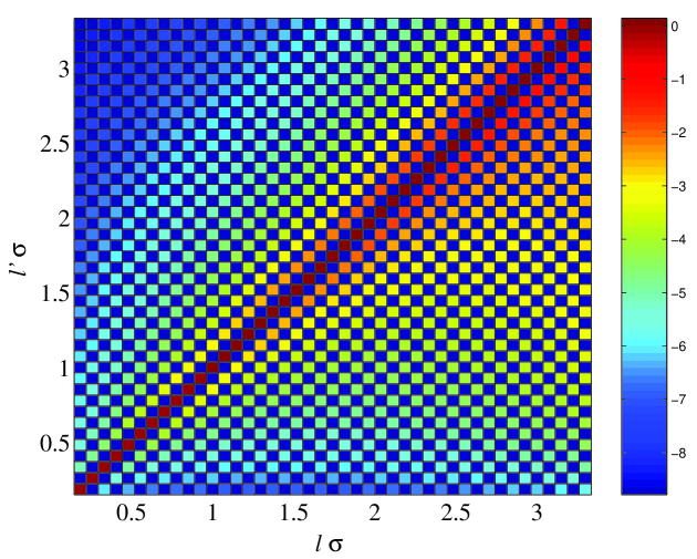
Figure 3: The log of normalized bias matrix $A_{ll^{\prime}}/(B_{l}B_{l^{\prime}})$ is plotted for an elliptical beam of eccentricity $e=0.6$ and mean beam-width $\bar{\sigma}=0.074$. The normalization is carried out so that the effect of non-circularity on the bias matrix can be easily compared to that for circular beams. Beam rotation and cut-sky effects have not been considered in this figure. One notices that the off-diagonal elements of the bias matrix take significant values for $l\bar{\sigma}\geq 1$.

The bias matrix including the leading order beam distortion (for non-rotating, reflection symmetric beams) can be summarized as

$\bullet$ For odd values of $l+{l^{\prime}}$,

$$A_{ll^{\prime}}\ =\ 0.$$ (42)

$\bullet$ For even values of $l+l^{\prime}$,

$$A_{l{l^{\prime}}}\ =\ \left\{\begin{array}[]{ll}(B_{l^{\prime}}\beta_{{l^{\prime}}2})^{2}\left(\frac{8\,l(l+1)(2l^{\prime}+1)}{l^{\prime 2}(l^{\prime}+1)^{2}(l^{\prime}-1)(l^{\prime}+2)}\right)\left[2\,+\,\sum_{m=1}^{l}\frac{(l+m)!(l^{\prime}-m)!}{(l-m)!(l^{\prime}+m)!}(m+1)^{2}\right]&\mbox{if $l<l^{\prime}$}\\ \\ (B_{l^{\prime}}\beta_{{l^{\prime}}2})^{2}\left(\frac{8\,l(l+1)(2l^{\prime}+1)}{l^{\prime 2}(l^{\prime}+1)^{2}(l^{\prime}-1)(l^{\prime}+2)}\right)\left[\sum_{m=1}^{l^{\prime}}\frac{(l-m)!(l^{\prime}+m)!}{(l+m)!(l^{\prime}-m)!}(m-1)^{2}\right]&\mbox{if $l>l^{\prime}$}\\ \\ \frac{B_{l}^{2}}{2l+1}\left[\left\{1-2\beta_{l2}\,\sqrt{\frac{l(l-1)}{(l+1)(l+2)}}\right\}^{2}+2\sum_{m=1}^{l}\left\{1-2\beta_{l2}\,\frac{(l^{2}+l+1)-(2l+1)m}{\sqrt{(l-1)l(l+1)(l+2)}}\right\}^{2}\right]&\mbox{if $l=l^{\prime}$}.\end{array}\right.$$ (43)

The non-zero off-diagonal terms in the bias matrix $A_{l{l^{\prime}}}$ imply that the non-circular beam mixes the contribution of different multipoles from the actual power spectrum in the observed power spectrum. Off-diagonal elements in $A_{l{l^{\prime}}}$ that arise from non-uniform/incomplete sky coverage have been studied earlier and are routinely accounted for in CMB experiments. Non-circular beam is yet another source of off-diagonal terms in the bias matrix and should be similarly taken into account. In general, CMB experiments have both non-circular beams and non-uniform/incomplete sky coverage that could lead to interesting features in $A_{l{l^{\prime}}}$.

Although the analytical result is limited to mildly non-circular and non-rotating beam functions, it does bring to light certain generic features of the effect of non-circular beam functions. To be specific, we compute the elements $A_{l{l^{\prime}}}$ for non-rotating elliptic Gaussian beams (see appendix A). The non-circularity of these beams is characterized by their eccentricity $e=\sqrt{1-\sigma_{2}^{2}/\sigma_{1}^{2}}$, where $\sigma_{1}$ and $\sigma_{2}$ are the $1\sigma$ beam-widths along major and minor axes of the beam (see table LABEL:tab:2). Many experiments have characterized their beams in terms of an elliptic Gaussian fit (e.g.,pyV ; whu01 ; fos02 ). A convenient advantage of elliptical beams is that the beam transform $b_{lm}$ (and obviously, the beam distortion parameters, $\beta_{lm}$) can be expressed in a closed analytical form. The results expressed in terms of $l\bar{\sigma}$ are broadly independent of the average beam-size TR:2001 .

Fig. 3 shows a density plot of the normalized bias matrix $A_{l{l^{\prime}}}/(B_{l}B_{l^{\prime}})$ for a non-rotating elliptical beam. The plot illustrates the importance of off-diagonal terms that arise due to the non-circular beam relative to the diagonal terms. The absence of coupling between multipoles separated by odd integers is evident. Also evident is the fall off as one moves away from the diagonal. The left panel of Fig. 4 shows that the off-diagonal elements of $A_{l{l^{\prime}}}$ are important at $l\bar{\sigma}\sim 1$. The results are qualitatively independent of the average beam size $\bar{\sigma}$. The right panel Fig. 4 shows the strong dependence of the dominant off-diagonal element $A_{l\,l+2}$ on the eccentricity of the beam.

The analytical results and numerical computations using eq. (26) were compared. The numerical and analytical results match perfectly as shown in Figure 4. Numerical computation involves the pixelized sky and the algorithm must ensure that this does not introduce spurious effects. We verify that $A_{l{l^{\prime}}}$ has numerically negligible off-diagonal elements when the beam is circularly symmetric. The numerical computation for non-circular beam are verified to be robust to the pixelization of the sky.

Next we illustrate effect of beam-rotation and non-uniform sky coverage for a hypothetical experiment where $A_{l{l^{\prime}}}$ have been computed numerically. The left panel of Fig. 5 shows (in $log$ scale) the normalized bias matrix arising from a $2.5^{\circ}$ circular beam including a non trivial $w(\mathbf{\hat{q}})$ in the form of a smoothed version of the galactic mask Kp2 of WMAP Bennett:2003 ; LamdaBl . The right panel of the figure shows the extra effect that a rotating non-circular beam would introduce. We assume a simple ‘toy’ beam rotation along an equal declination scan strategy, where the beam continuously ‘rotates’ by $2\pi$ for every complete pass at a given declination which implies the simple form

$$\rho(\mathbf{\hat{q}})\equiv\rho(\theta,\phi)=\phi\,.$$ (44)

The elements here have been computed numerically using eq. (26) retaining the leading order terms in the perturbation expansion of $W_{l}$ in eq. (18). The off-diagonal effects at low $l$ are dominated by the cut sky effect. The off-diagonal element $l\bar{\sigma}\mathrel{\hbox to0.0pt{\lower 4.0pt\hbox{\hskip 1.0pt$\sim$}\hss}\raise 1.0pt\hbox{$>$}}1$ arise solely due to non-circular beam. The numerical computation illustrates the potentially large corrections that can arise due to non-circular beam that ‘rotate’ on the sky. The numerical computations in this work pave the way for introducing realistic scan-pattern, beam-rotation and non-uniform sky coverage in a future extension to our work.

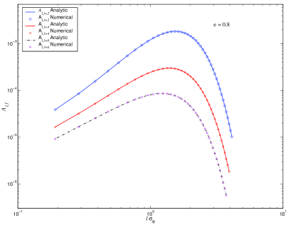
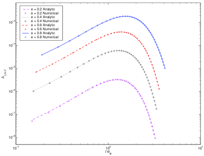
Figure 4: Elements of the bias matrix $A_{l{l^{\prime}}}$ are plotted in this figure as a function of multipole $(l)$. The bias matrix relates the observed $\mathcal{C}_{l}$s to their true values. When non-circular beams are used in CMB experiments, the bias matrix can be shown to be non-diagonal, thus implying mixing of power between multipoles. On the left panel, we plot $A_{l{l^{\prime}}}$ for ${l^{\prime}}-l=2,4,6$. It is evident that the effect decreases as we move away from the diagonal and that it kicks in at $l\bar{\sigma}\sim 1$, for a beam of eccentricity $e=0.8$. For the figure in the right panel, we plot $A_{l\,l+2}$ for several beams of the same size but different eccentricities. Clearly, the effect also depends strongly on the non-circularity of the beam.

We summarize the following features of the bias matrix :

1. There is no coupling between $\langle\widetilde{\mathcal{C}}_{l}\rangle$ and $\mathcal{C}_{l^{\prime}}$ for odd values of $l+{l^{\prime}}$,

2. Coupling decreases as $|l-{l^{\prime}}|$ increases,

3. Coupling increases with eccentricity for fixed beam size, and

4. Size of the beam determines the multipole $l$ value for which coupling will be maximum ($l\bar{\sigma}\sim 1$).
   

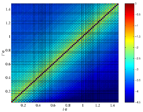
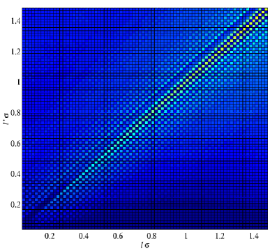
Figure 5: The normalized bias matrix elements (on log scale, $\log[A_{l{l^{\prime}}}/(B_{l}B_{l^{\prime}})]$) of a hypothetical experiment with a scan pattern (eq. 44) corresponding to a rotating, non circular beam ($e=0.6$) and non uniform sky coverage are studied. The left panel shows the effect of non-uniform coverage alone (circular beam approximation). The right panel isolates the additional effect that arises due to the non-circularity of the beam and its rotation. We note that significant off-diagonal elements arise at $l\bar{\sigma}\geq 1$ from the non-circular beam comparable to that from the non-uniform coverage. The non-uniform coverage corresponds to a smoothed WMAP Kp2 galactic mask (smoothed from resolution of $N_{side}=512$ to $64$). We use a sufficiently high resolution beam with $\bar{\sigma}=0.018$ ($\theta_{1/2}=2.5^{\circ}$) to ensure that the effects due to the galactic mask and the non-circular beam appear in distinct regions of the multipole space.

Figure 6 roughly indicates the level and nature of the effect of neglecting the non-circularity of the beam on CMB power estimation (for the conservative case of non-rotating beams). Consider the power spectrum $\widetilde{\mathcal{C}}_{l}=\sum_{{l^{\prime}}}\,A_{l{l^{\prime}}}\mathcal{C}_{l^{\prime}}$ measured using a non-circular, elliptical Gaussian beam of a given eccentricity, $e$ and average beam-width, $\bar{\sigma}$. We compare the power spectrum obtained by deconvolving $\widetilde{\mathcal{C}}_{l}$ with a circular, Gaussian beam of the beam-width, $\bar{\sigma}$ with the true $\mathcal{C}_{l}$. The lower panel shows that the error can be significant for multipole values beyond the inverse beam-width even for modestly non-circular comparable to the WMAP beam maps (Q-band) discussed in the Appendix A.

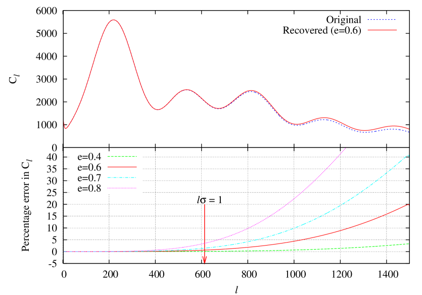
Figure 6: The effect of non-circular beam is studied for CMB power spectrum estimation by a CMB experiment with a WMAP-like non-circular beam. For illustration, we consider the best fit (Power law) model to be the (fiducial) true $\mathcal{C}_{l}$ of the Universe shown as the solid line in the upper panel. Let $\widetilde{\mathcal{C}}_{l}$ be the power spectrum measured by using a elliptical, Gaussian beam with eccentricity, $e=0.6$, and $\bar{\sigma}=0.0016$. The dashed line shows the $\mathcal{C}_{l}$ that would be inferred by deconvolving $\widetilde{\mathcal{C}}_{l}$ with a circular beam assumption with beam-width, $\bar{\sigma}$. The lower panel plots the relative error in the power spectrum recovered with a circular beam assumption for a measurements made with a non-circular beam with $e=0.4$ to $0.8$.

Finally, we construct the unbiased estimator for the angular power spectrum. Invoking steps similar to the case of circular beams to account for the instrumental noise, we obtain

$$\langle\widetilde{\mathcal{C}}_{l}^{\prime}\rangle\ =\ \langle\widetilde{\mathcal{C}}_{l}\rangle\ +\ \mathcal{C}_{l}^{N}\ =\ \sum_{l^{\prime}}A_{l{l^{\prime}}}\mathcal{C}_{l^{\prime}}\ +\ \mathcal{C}_{l}^{N}.$$ (45)

The unbiased estimator for the angular power spectrum is

$$\widetilde{\mathcal{C}}_{l}^{UB}\ =\ \sum_{l^{\prime}}\,A_{l{l^{\prime}}}^{-1}\left(\widetilde{\mathcal{C}}_{l^{\prime}}^{\prime}\ -\ \mathcal{C}_{l^{\prime}}^{N}\right).$$ (46)

IV Error-Covariance Matrix

The statistical error-covariance of the estimated angular power spectrum is defined as

$$\mbox{Cov}(\widetilde{\mathcal{C}}_{l},\widetilde{\mathcal{C}}_{l^{\prime}})\ \equiv\ \langle(\widetilde{\mathcal{C}}_{l}-\langle\widetilde{\mathcal{C}}_{l}\rangle)(\widetilde{\mathcal{C}}_{l^{\prime}}-\langle\widetilde{\mathcal{C}}_{l^{\prime}}\rangle)\rangle.$$ (47)

In an idealized, noise free, CMB experiment with infinite angular resolution uniformly covering the full sky

$$\widetilde{\mathcal{C}}_{l}\ =\frac{l(l+1)}{8\pi^{2}}\int d\Omega_{\mathbf{\hat{q}}_{1}}\int d\Omega_{\mathbf{\hat{q}}_{2}}\Delta T(\mathbf{\hat{q}}_{1})\Delta T(\mathbf{\hat{q}}_{2})P_{l}(\mathbf{\hat{q}}_{1}\cdot\mathbf{\hat{q}}_{2}).$$ (48)

Using the property of Gaussian random fields that,

$$\langle\Delta T(\mathbf{\hat{q}}_{1})\Delta T(\mathbf{\hat{q}}_{2})\Delta T(\mathbf{\hat{q}^{\prime}}_{1})\Delta T(\mathbf{\hat{q}^{\prime}}_{2})\rangle = \langle\Delta T(\mathbf{\hat{q}}_{1})\Delta T(\mathbf{\hat{q}}_{2})\rangle\langle\Delta T(\mathbf{\hat{q}^{\prime}}_{1})\Delta T(\mathbf{\hat{q}^{\prime}}_{2})\rangle+$$

$$\langle\Delta T(\mathbf{\hat{q}}_{1})\Delta T(\mathbf{\hat{q}^{\prime}}_{1})\rangle\langle\Delta T(\mathbf{\hat{q}}_{2})\Delta T(\mathbf{\hat{q}^{\prime}}_{2})\rangle+\langle\Delta T(\mathbf{\hat{q}}_{1})\Delta T(\mathbf{\hat{q}^{\prime}}_{2})\rangle\langle\Delta T(\mathbf{\hat{q}^{\prime}}_{1})\Delta T(\mathbf{\hat{q}}_{2})\rangle$$

and eq. (6), we recover the well known result for full sky CMB maps

$$\mbox{Cov}(\widetilde{\mathcal{C}}_{l},\widetilde{\mathcal{C}}_{l^{\prime}})\ =\ \frac{2}{2l+1}\,\langle\mathcal{C}_{l}\rangle^{2}\,\delta_{l{l^{\prime}}}\ =\ \frac{2}{2l+1}\,\mathcal{C}_{l}^{2}\,\delta_{l{l^{\prime}}}\,,$$ (50)

corresponding to $C_{l}$ being a sum of the squares of $2l+1$ Gaussian variates, i.e. $\chi^{2}_{2l+1}$ distribution. The measured power spectrum at each multipole is independent (for full sky CMB maps). The variance of the power spectrum estimator is not zero even in the ideal case. Consequently, the measurement angular power spectrum from the one available CMB sky map is inherently limited by an inevitable error the Cosmic Variance .

IV.1 Circular Beam

For measurements made with a circular beam, the temperature is a linear transform of the actual temperature (see eq. (7)). So, it also represents a Gaussian random field. Hence, eq. (IV) remains valid even for observed temperature fluctuations. Moreover, the window function takes a simple form given in eq. (11). Consequently, eq. (6) gets modified to

$$\langle\widetilde{\Delta T}(\mathbf{\hat{q}}_{1})\widetilde{\Delta T}(\mathbf{\hat{q}}_{2})\rangle\ =\ \sum_{l=0}^{\infty}\frac{2l+1}{2l(l+1)}\,B_{l}^{2}\,\mathcal{C}_{l}\,P_{l}(\mathbf{\hat{q}}_{1}\cdot\mathbf{\hat{q}}_{2}).$$ (51)

The covariance matrix

$$\mbox{Cov}(\widetilde{\mathcal{C}}_{l},\widetilde{\mathcal{C}}_{l^{\prime}})\ =\ \frac{2}{2l+1}\,\langle\widetilde{\mathcal{C}}_{l}\rangle^{2}\delta_{l{l^{\prime}}}\ =\ \frac{2}{2l+1}\,(B_{l}^{2}\mathcal{C}_{l})^{2}\,\delta_{l{l^{\prime}}},$$ (52)

remains diagonal for circular beams, i.e., the measured power spectrum at each multipole is independent of the power measured in the other multipoles. The second equality follows from eq. (28).

Including the instrumental noise spectrum in the measured power spectrum $\mathcal{C}_{l}^{N}$, we obtain

$$\mbox{Cov}(\widetilde{\mathcal{C}}_{l}^{\prime},\widetilde{\mathcal{C}}_{l^{\prime}}^{\prime})\ =\ \frac{2\delta_{l{l^{\prime}}}}{2l+1}\left(\langle\widetilde{\mathcal{C}}_{l}\rangle+\mathcal{C}_{l}^{N}\right)^{2},$$ (53)

where we assume that the noise spectrum $\mathcal{C}_{l}^{N}$ is known much better and, in particular, does not suffer from cosmic variance. For the unbiased estimator given by eq. (31), the well known covariance matrix

$$\mbox{Cov}(\widetilde{\mathcal{C}}_{l}^{UB},\widetilde{\mathcal{C}}_{l^{\prime}}^{UB})\ =\ B_{l}^{-4}\mbox{Cov}(\widetilde{\mathcal{C}}_{l}^{\prime},\widetilde{\mathcal{C}}_{l^{\prime}}^{\prime})\ =\ \frac{2\delta_{l{l^{\prime}}}}{2l+1}\left(\mathcal{C}_{l}+B_{l}^{-2}\mathcal{C}_{l}^{N}\right)^{2}$$ (54)

is readily obtained from the linear transformation between $\mathcal{C}_{l}^{\prime}$ and $\mathcal{C}_{l}^{UB}$ knox95 ; bonLH .

IV.2 Non-circular Beam

As expected, the covariance for the non-circular beam is considerably more complicated. We start with the general form of the two point correlation function. Using eq. (24), the general form of the covariance matrix is

$$\mbox{Cov}(\widetilde{\mathcal{C}}_{l},\widetilde{\mathcal{C}}_{l^{\prime}}) = \frac{l{l^{\prime}}(l+1)({l^{\prime}}+1)}{(4\pi)^{4}}\sum_{l_{1},l_{2}=0}^{\infty}\frac{(2l_{1}+1)(2l_{2}+1)}{l_{1}l_{2}(l_{1}+1)(l_{2}+1)}\,\mathcal{C}_{l_{1}}\mathcal{C}_{l_{2}}\,\int d^{4}\Omega w(\mathbf{\hat{q}}_{1})w(\mathbf{\hat{q}}_{2})w(\mathbf{\hat{q}^{\prime}}_{1})w(\mathbf{\hat{q}^{\prime}}_{2})\times$$ (55)

$$P_{l}(\mathbf{\hat{q}}_{1}\cdot\mathbf{\hat{q}}_{2})P_{l^{\prime}}(\mathbf{\hat{q}^{\prime}}_{1}\cdot\mathbf{\hat{q}^{\prime}}_{2})\,[W_{l_{1}}(\mathbf{\hat{q}}_{1},\mathbf{\hat{q}^{\prime}}_{1})W_{l_{2}}(\mathbf{\hat{q}}_{2},\mathbf{\hat{q}^{\prime}}_{2})\,+\,W_{l_{1}}(\mathbf{\hat{q}}_{1},\mathbf{\hat{q}^{\prime}}_{2})W_{l_{2}}(\mathbf{\hat{q}}_{2},\mathbf{\hat{q}^{\prime}}_{1})],$$

where for brevity we denote $d^{4}\Omega\ \equiv\ d\Omega_{\mathbf{\hat{q}}_{1}}d\Omega_{\mathbf{\hat{q}}_{2}}d\Omega_{\mathbf{\hat{q}^{\prime}}_{1}}d\Omega_{\mathbf{\hat{q}^{\prime}}_{2}}$.

Noting the interchangeability of the dummy variables $\mathbf{\hat{q}^{\prime}}_{1}$ and $\mathbf{\hat{q}^{\prime}}_{2}$, we combine the two terms in the above equation to obtain

$$\mbox{Cov}(\widetilde{\mathcal{C}}_{l},\widetilde{\mathcal{C}}_{l^{\prime}}) = 2\left[\frac{l{l^{\prime}}(l+1)({l^{\prime}}+1)}{(4\pi)^{4}}\right]\sum_{l_{1},l_{2}=0}^{\infty}\frac{(2l_{1}+1)(2l_{2}+1)}{l_{1}l_{2}(l_{1}+1)(l_{2}+1)}\,\mathcal{C}_{l_{1}}\mathcal{C}_{l_{2}}\,\times$$ (56)

$$\int d^{4}\Omega w(\mathbf{\hat{q}}_{1})w(\mathbf{\hat{q}}_{2})w(\mathbf{\hat{q}^{\prime}}_{1})w(\mathbf{\hat{q}^{\prime}}_{2})P_{l}(\mathbf{\hat{q}}_{1}\cdot\mathbf{\hat{q}}_{2})P_{l^{\prime}}(\mathbf{\hat{q}^{\prime}}_{1}\cdot\mathbf{\hat{q}^{\prime}}_{2})W_{l_{1}}(\mathbf{\hat{q}}_{1},\mathbf{\hat{q}^{\prime}}_{1})W_{l_{2}}(\mathbf{\hat{q}}_{2},\mathbf{\hat{q}^{\prime}}_{2}).$$

We expand the Legendre Polynomials in terms of spherical harmonics (eq. (5)) and use the expression for the window function in eq. (15) to obtain

$$\mbox{Cov}(\widetilde{\mathcal{C}}_{l},\widetilde{\mathcal{C}}_{l^{\prime}})=\frac{l{l^{\prime}}(l+1)({l^{\prime}}+1)}{8\pi^{2}(2l+1)(2{l^{\prime}}+1)}\sum_{l_{1},l_{2}=0}^{\infty}\frac{(2l_{1}+1)(2l_{2}+1)}{l_{1}l_{2}(l_{1}+1)(l_{2}+1)}\,\mathcal{C}_{l_{1}}\mathcal{C}_{l_{2}}B_{l_{1}}^{2}B_{l_{2}}^{2}\sum_{m=-l}^{l}\sum_{m^{\prime}=-{l^{\prime}}}^{{l^{\prime}}}\sum_{m_{1}=-l_{1}}^{l_{1}}\sum_{m_{2}=-l_{2}}^{l_{2}}$$

$$\left[\sum_{m^{\prime}_{1},m^{\prime\prime}_{1}=-l_{1}}^{l_{1}}\beta_{l_{1}m^{\prime}_{1}}\beta_{l_{1}m^{\prime\prime}_{1}}^{*}\int d\Omega_{\mathbf{\hat{q}}_{1}}w(\mathbf{\hat{q}}_{1})Y_{lm}^{*}(\mathbf{\hat{q}}_{1})D_{m_{1}m^{\prime}_{1}}^{l_{1}}(\mathbf{\hat{q}}_{1},\rho(\mathbf{\hat{q}}_{1}))\int d\Omega_{\mathbf{\hat{q}^{\prime}}_{1}}w(\mathbf{\hat{q}^{\prime}}_{1})Y_{{l^{\prime}}m^{\prime}}(\mathbf{\hat{q}^{\prime}}_{1})D_{m_{1}m^{\prime\prime}_{1}}^{l_{1}*}(\mathbf{\hat{q}^{\prime}}_{1},\rho(\mathbf{\hat{q}^{\prime}}_{1}))\right.$$

$$\left.\sum_{m^{\prime}_{2},m^{\prime\prime}_{2}=-l_{2}}^{l_{2}}\beta_{l_{2}m^{\prime}_{2}}^{*}\beta_{l_{2}m^{\prime\prime}_{2}}\int d\Omega_{\mathbf{\hat{q}}_{2}}w(\mathbf{\hat{q}}_{2})Y_{lm}(\mathbf{\hat{q}}_{2})D_{m_{2}m^{\prime}_{2}}^{l_{2}*}(\mathbf{\hat{q}}_{2},\rho(\mathbf{\hat{q}}_{2}))\int d\Omega_{\mathbf{\hat{q}^{\prime}}_{2}}w(\mathbf{\hat{q}^{\prime}}_{2})Y_{{l^{\prime}}m^{\prime}}^{*}(\mathbf{\hat{q}^{\prime}}_{2})D_{m_{2}m^{\prime\prime}_{2}}^{l_{2}}(\mathbf{\hat{q}^{\prime}}_{2},\rho(\mathbf{\hat{q}^{\prime}}_{2}))\right]\,,$$

(57)

as the general expression for error covariance for angular power spectrum for non-circular beams. Note that even for full, uniform sky observations, $w(\mathbf{\hat{q}})=1$, the error covariance matrix is no longer diagonal.

To make further progress analytically, we restrict to the case of uniform, full sky coverage ($w(\mathbf{\hat{q}})=1$) with no beam rotation ($\rho(\mathbf{\hat{q}})=0$). Using the integration of eq. (33) and after a considerable algebra we may write the expression for covariance as

$$\mbox{Cov}(\widetilde{\mathcal{C}}_{l},\widetilde{\mathcal{C}}_{l^{\prime}})=\frac{l{l^{\prime}}(l+1)({l^{\prime}}+1)}{8}\sum_{m=-L}^{L}\left[\sum_{l_{1}=|m|}^{\infty}B_{l_{1}}^{2}\mathcal{C}_{l_{1}}\frac{(2l_{1}+1)}{l_{1}(l_{1}+1)}\sum_{m^{\prime}_{1}=-l_{1}}^{l_{1}}\beta_{l_{1}m^{\prime}_{1}}I_{mm^{\prime}_{1}}^{ll_{1}}\sum_{m^{\prime\prime}_{1}=-l_{1}}^{l_{1}}\beta_{l_{1}m^{\prime\prime}_{1}}^{*}I_{mm^{\prime\prime}_{1}}^{{l^{\prime}}l_{1}}\right]^{2}$$ (58)

where $L={\rm min}\{l,{l^{\prime}}\}$ is the smaller between $l$ and ${l^{\prime}}$. The integrals $I_{mm^{\prime}}^{l{l^{\prime}}}$ are defined in §III and the analytical expressions for $m^{\prime}=0,\pm 2$ are given. It is straightforward to verify that the above equation correctly reproduces the expression for the error-covariance in the circular beam case given by eq. (52).

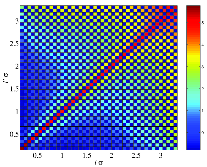
Figure 7: Log of the normalized covariance matrix Cov$(C_{l},C_{l^{\prime}})/(B_{l}B_{l^{\prime}})^{2}$ [in the units of $(\mu K)^{4}$] is plotted for an elliptical beam of eccentricity $e=0.6$ and mean beam-width $\bar{\sigma}=0.074$. Due to the non-circularity of the beam, the error in CMB angular power spectrum estimate at different multipoles are no longer independent. We notice that the off-diagonal elements of the error covariance matrix are pronounced for $l\bar{\sigma}\geq 1$.

For evaluation of the covariance matrix, we note that though the summation over $l_{1}$ runs from $0$ to $\infty$, the contributions are significant only around $l\sim 1/\bar{\sigma}$ and the summation can be truncated suitably. Further, for most beams we can confine to the leading order approximation as in eq. (18), by neglecting all the $\beta_{lm}$’s for $m\geq 4$. For mild deviations from circular beams, the observed power spectrum at different multipoles are weakly correlated ( $\sim\beta_{l2}\beta_{{l^{\prime}}2}$). The error-covariance matrix can be diagonalized to find the independent linear combinations of estimators (eigenvectors), and the variances of theses independent estimators are given by the corresponding eigenvalues. These eigenvalues are necessarily larger that the cosmic variance corresponding to a circular beam.

The inclusion of instrumental noise is similar to what was done in the circular beam case. The covariance

$$\mbox{Cov}(\widetilde{\mathcal{C}}_{l}^{\prime},\widetilde{\mathcal{C}}_{l^{\prime}}^{\prime})\ =\ \mbox{Cov}(\widetilde{\mathcal{C}}_{l},\widetilde{\mathcal{C}}_{l^{\prime}})\ +\ \frac{2\delta_{l{l^{\prime}}}}{2l+1}\left[2\langle\widetilde{\mathcal{C}}_{l}\rangle\mathcal{C}_{l}^{N}\,+\,(\mathcal{C}_{l}^{N})^{2}\right]$$ (59)

clearly reproduces the result in eq. (52) in the limit of a circular beam. Figure 7 shows a density plot of the elements of the covariance matrix for a non-circular (elliptical) beam with no rotation. In contrast to the case for incomplete (cut) sky case, where the effects are at small $l$ (see efs04 ), the non-circular beam affects the large multipoles region ($l\bar{\sigma}\geq 1$). The pseudo-$C_{l}$ approach is close to optimal for large $l$ hence it may be more important to account for non-circular beams effects than the cut-sky, since it is possible to use maximum likelihood estimator for small $l$.

The error-covariance matrix for the unbiased estimator eq. (46) for non-circular beams is given by

$$\mbox{Cov}(\widetilde{\mathcal{C}}_{l}^{UB},\widetilde{\mathcal{C}}_{l^{\prime}}^{UB}) = \sum_{l_{1}}\sum_{l_{2}}A_{ll_{1}}^{-1}A_{{l^{\prime}}l_{2}}^{-1}\mbox{Cov}(\widetilde{\mathcal{C}}_{l_{1}}^{\prime},\widetilde{\mathcal{C}}_{l_{2}}^{\prime})$$ (60)

$$= \sum_{l_{1}}\sum_{l_{2}}\alpha_{ll_{1}}\alpha_{{l^{\prime}}l_{2}}(B_{l_{1}}B_{l_{2}})^{-2}\left[\mbox{Cov}(\widetilde{\mathcal{C}}_{l},\widetilde{\mathcal{C}}_{l^{\prime}})\ +\ \frac{2\delta_{l{l^{\prime}}}}{2l+1}\left\{2\langle\widetilde{\mathcal{C}}_{l}\rangle\mathcal{C}_{l}^{N}\,+\,(\mathcal{C}_{l}^{N})^{2}\right\}\right],$$

where the matrix $\alpha_{l{l^{\prime}}}\equiv B_{{l^{\prime}}}^{-2}A_{l{l^{\prime}}}^{-1}$, being very close to identity, demonstrates that the beam-modified cosmic variance part of the covariance of unbiased estimator weakly depends on $B_{l}$’s, whereas the noise part depends on them significantly.

V Discussion and Conclusion

We present an analytic framework for addressing the effect of non-circular experimental beam function in the estimation of the angular power spectrum $\mathcal{C}_{l}$ of CMB anisotropy. Non-circular beam effects can be modeled into the covariance functions in approaches related to maximum likelihood estimation max97 ; bjk98 and can also be included in the Harmonic ring harm02 and ring-torus estimators wan_han03 . The latter is promising since it reduces the computational costs from $N^{3}$ to $N^{2}$. However, all these methods are computationally prohibitive for high resolution maps and, at present, the computationally economical approach of using a pseudo-$C_{l}$ estimator appears to be a viable option for extracting the power spectrum at high multipoles efs04 . The pseudo-$C_{l}$ estimates have to be corrected for the systematic biases. While considerable attention has been devoted to the effects of incomplete/non-uniform sky coverage, no comprehensive or systematic approach is available for non-circular beam. The high sensitivity, ‘full’ (large) sky observation from space (long duration balloon) missions have alleviated the effect of incomplete sky coverage and other systematic effects such as the one we consider here have gained more significance. Non-uniform coverage, in particular, the galactic masks affect only CMB power estimation at the low multipoles. Recently proposed hybrid scheme promotes a strategy where the power spectrum at low multipoles is estimated using optimal Maximum Likelihood methods and pseudo-$C_{l}$ are used for large multipoles.

We have shown that non-circular beam is an effect that dominates at large $l$ comparable to the inverse beam width. For high resolution experiment, the optimal maximum likelihood methods which can account for non-circular beam functions are computationally prohibitive. In implementing pseudo-$C_{l}$ estimation, the non-circular beam effect could dominate over the effects of more well studied effect of non-uniform sky coverage. Our work provides a convenient approach for estimating the magnitude of this effect in terms of the leading order deviations from a circular beam. The perturbation approach is very efficient. For most CMB experiments the leading few orders capture most of the effect of beam non-circularity. The perturbation approach has allowed the development of computationally rapid method of computing window functions TR:2001 . Our work may similarly yield computationally rapid methods correcting for beam non-circularity.

The quantitative estimates of the off-diagonal matrix elements of the bias and error-covariance for ‘non-rotating’ beam graphically illustrate the general features that can be gleaned from our analytic results. They show that the beam non-circularity affects the $C_{l}$ estimation on multipoles larger than the inverse beam width. A strong dependence on the eccentricity of the beam is also seen. We caution against interpreting these results as a measure of the non-circular beam effects for any real CMB experiment. The analytical results are limited to non-rotating beams and uniform sky coverage. Numerical results do not include scan pattern of any known experiment. Numerical calculations of the bias matrix for a ‘toy’ scanning strategy where the beam rotates on the sky indicates the possibility of significant corrections. The bias due to non-uniform sky coverage can have interesting coupling to the bias from beam non-circularity. On the other hand, it has also been shown that effects of non-circular beams can be diluted if the scan pattern is such that each point in the sky is revisited by the beam with a different orientation at different time whu01 . The numerical implementation of our method can readily accommodate the case when pixels are revisited by the beam with different orientations. Evaluating the realistic bias and error-covariance for a specific CMB experiment with non-circular beams would require numerical evaluation of the general expressions for $A_{l{l^{\prime}}}$ in eqs. (27) using real scan strategy and account for inhomogeneous noise and sky coverage. We defer such an exercise to future work.

It is worthwhile to note in passing that that the angular power $C_{l}$ contains all the information of Gaussian CMB anisotropy only under the assumption of statistical isotropy. Gaussian CMB anisotropy map measured with a non-circular beam corresponds to an underlying correlation function that violates statistical isotropy. In this case, the extra information present may be measurable using, for example, the bipolar power spectrum haj_sour03 . Even when the beam is circular the scanning pattern itself is expected to cause a breakdown of statistical isotropy of the measured CMB anisotropy  master . For a non-circular beam, this effect could be much more pronounced and, perhaps, presents an interesting avenue of future study.

In addition to temperature fluctuations, the CMB photons coming from different directions have a random, linear polarization. The polarization of CMB can be decomposed into $E$ part with even parity and $B$ part with odd parity. Besides the angular spectrum $C_{l}^{TT}$, the CMB polarization provides three additional spectra, $C_{l}^{TE}$, $C_{l}^{EE}$ and $C_{l}^{BB}$ which are invariant under parity transformations. The level of polarization of the CMB being about a tenth of the temperature fluctuation, it is only very recently that the angular power spectrum of CMB polarization field has been detected. The Degree Angular Scale Interferometer (DASI) has measured the CMB polarization spectrum over limited band of angular scales in late 2002 kov_dasi02 . The WMAP mission has also detected CMB polarization kog_wmap03 . WMAP is expected to release the CMB polarization maps very soon. Correcting for the systematic effects of a non-circular beam for the polarization spectra is expected to become important soon. Our work is based on the perturbation approach of  TR:2001 which has been already been extended to the case of CMB polarization fos02 . Extending this work to the case CMB polarization is another line of activity we plan to undertake in the near future.

In summary, we have presented a perturbation framework to compute the effect of non-circular beam function on the estimation of power spectrum of CMB anisotropy. We not only present the most general expression including non-uniform sky coverage as well as a non-circular beam that can be numerically evaluated but also provide elegant analytic results in interesting limits. In this work, we have skipped over the effect of non-circular beam functions on map-making step. In simple scanning strategies, our results may be readily applied in this context. As CMB experiments strive to measure the angular power spectrum with increasing accuracy and resolution, the work provides a stepping stone to address a rather complicated systematic effect of non-circular beam functions.

Appendix A Elliptical Gaussian fit to the WMAP beam maps

We briefly describe an exercise in characterizing non-circular beams in CMB experiments using the beam maps of the WMAP mission. We analyzed the WMAP raw beam images in the Q1, V1 and W1 LamdaBl ; pag03 bands using two different standard software packages. We use the elliptical Gaussian fit allowed by the well known radio-astronomy software, AIPS and a more elaborate ellipse fitting routine available within the standard astronomical image/data processing software IRAF. The ELLIPSE task in the STSDAS package of IRAF, which uses the widely known ellipse fitting routines by Jedrzejewski iraf , allows independent elliptical fits to the isophotes. This significant greater degree of freedom in fitting to the non-circular beam allows us to assess whether a simple elliptical Gaussian fit is sufficient. The three bands see Jupiter in the two horns (labeled A and B) as a point source. The fitting routine fits ellipses along iso-intensity contours of the beam image, parameterized by position angle (PA), ellipticity ($\bar{\epsilon}$) and position of the center. Each of these parameters can be independently varied. The distance between successive ellipses can also be independently varied. The eccentricity $e$ is related to ellipticity $\bar{\epsilon}$ as $e=\sqrt{1-(1-\bar{\epsilon})^{2}}$ (Please see Table LABEL:tab:2).

Figure 8: The beam profile is characterized by intensity along the semi major axis (SMA). The beam in Q-band for WMAP experiment was analyzed using IRAF and fitted to both circular and elliptical profiles. We have plotted the best fit circular profile (solid error bars) and overlaid the profile recovered by inverting the WMAP beam transforms, available at LAMBDA website (solid line). Two analytical models for circular beam profile $g(\theta)$ and $h(\theta)$ are also considered, and the best fit profiles are overlaid. We find that these models are consistent with the IRAF and WMAP data. We have also plotted the best fit elliptical profile along SMA (broken error bar). Notice that the error bars in this case are much smaller than those for circular profile, implying a better agreement with the data.

We fit the the beams in two different ways: (a) by holding the ellipticity constant to $\bar{\epsilon}=0.05$ and freely varying the position angle and center and (b) fixing the center to be the pixel with the highest intensity (normalized to 1.0 at the central pixel) and varying ellipticity and position angle. In the first case, we get the closest approximation to circular beam profiles as used in WMAP data analysis. This beam has no azimuthal ($\phi$) dependence. In the latter case, we get the elliptical profile of the WMAP beam which depends on both the polar ($\theta$) and azimuthal ($\phi$) distance from the pointing direction. Notice that in this case it is sufficient to provide the intensity along a particular direction (usually, the semi-major axis or $\phi=0$) and the ellipticity $\bar{\epsilon}$.

Figure 9: The beams for WMAP experiment in three bands Q, V and W for both the horns (A and B) were fitted to elliptical profiles using IRAF. The plot above shows the fitted eccentricity and position angle along the semi major axis (SMA). The presence of side-bands in the smaller beams (W band) makes it difficult for IRAF to model them sufficiently well. However, in the Q1 band, such sub-structures in the beam are not present thus allowing the IRAF ellipse fitting routine to fit reasonably good ellipses which have consistent eccentricities ($e\sim 0.65$) and position angles all along the SMA. The V1 beam is smaller in extent than the Q1 beam and its eccentricity was determined to be $e\sim 0.46$ using IRAF. The highest resolution beam in in W1 band, whose eccentricity was determined to be $e\sim 0.40$.

Even a visual inspection reveals that the Q1 beam map plotted in Fig 2 is non-circular and the iso-intensity contours distinctly elliptical. Thus it comes as no surprise that the error bars as shown in Figure 8 for circularized beam are larger than those for the elliptical profile. As a consistency check, we take the WMAP Q1 beam transfer function $B_{l}$ from WMAP first year data archived at publicly available LAMBDA site LamdaBl and ‘recover’ the circular beam profile $B(\theta)$ using eq. (10).

From Figure 8, it is clear that this ‘recovered’ beam profile is in good agreement with that obtained by IRAF. This allows us to make some statements about the profile fitting in CMB experiments, in the context of WMAP beams. The beam profile $B(\theta)$ has been modeled as a Gaussian times a sum of even order Hermite polynomials ($H_{2n}$) by the WMAP team pag03 . To compare, we have also modeled the beam profile with a function $h(\theta)$ given by

$$h(\theta)=\exp\left(-\frac{1}{2}\ \alpha\theta^{2}\right)\left(h_{0}+h_{2}H_{2}(\theta)+h_{4}H_{4}(\theta)\right),$$ (61)

where $\alpha,h_{0},h_{2}$ and $h_{4}$ are unknown parameters to be fixed by least squared method. We found that this model fits the data very well with a reduced $\chi^{2}$ of about $0.7$. However, on closer analysis, it is found that the chief role of the Hermite polynomials is to add a constant baseline over and above the Gaussian. To test this hypotheses, we choose another form of the fitting function $g(\theta)$ given by

$$g(\theta)=g_{0}+g_{1}\exp\left(-\frac{1}{2}\ g_{2}\theta^{2}\right),$$ (62)

where $g_{0},g_{1}$ and $g_{2}$ are parameters of the model. It is very interesting to note that this model also fits the data very well with a reduced $\chi^{2}$ of about $0.8$ for the best fitted parameters. In all fairness, $g(\theta)$ serves as a simpler model for the beam profile. We cannot point to the precise origin for the baseline. However, such ‘skirts’ in beam responses are not uncommon in radio-astronomy. At this point, our observation should perhaps merit a curious aside, if not as an alternative approach to beam modeling. Our best-fit models $g(\theta)$ and $h(\theta)$, along with the IRAF fitted data points to the WMAP Q1 (A) beam is shown in Figure 8.

As shown earlier in this paper, the effects of non-circularity of the CMB experimental beams show up in the power-spectral density estimates through the off-diagonal elements of the bias matrix $A_{ll^{\prime}}$. As shown in eq. (27), these in turn can be expressed in terms of the leading components of the harmonic transform of the beam. In general the harmonic decomposition of a non-circular beam may have to be done numerically. But for the particular case of an elliptical Gaussian beam, a closed form expression given by eq. (20) serves as a useful test-bed for us. Thus another motivation for fitting ellipses to WMAP beams using IRAF was to get a handle on the eccentricity of these beams so as to find the harmonic transform components of an elliptical Gaussian beam of similar eccentricity. This allows us to give more realistic estimates of the effect of non-circularity of the beam on $C_{l}$ estimates.

Table 2: The result of ellipse fitting using IRAF on the Q1, V1 and W1 beams of the WMAP experiments. The frequency quoted is the ‘effective’ frequency of the corresponding band from Page et. al. pag03 . The presence of sub-structures in the W1 band makes it difficult to fit elliptical contours to the beam.

Beam	Frequency	Eccentricity	Position Angle
	(GHz)		(degree)
Q1 (A)	40.9	0.65	+80
Q1 (B)	40.9	0.67	-80
V1 (A)	60.3	0.48	+60
V1 (B)	60.3	0.45	-60
W1 (A)	93.5	0.40	—

It is interesting to note how the fitted eccentricities vary as a function of the distance along the semi-major axis of the fitted ellipses for various beams. The smaller beams (V1 and W1) have sufficient sub-structure in the form of side-lobes which throws the ellipse fitting routine off course. However, where the sub-structure is less pronounced, we find that the eccentricities of the fitted ellipses takes a constant value. Toward the center of the ellipses, there are far too few pixels to average over, which in turn manifests as large error bars in the eccentricities and position angles of the ellipses. In Figure 9, we notice that the Q1 beam has a very elliptical profile with eccentricity $e\mathrel{\hbox to0.0pt{\lower 4.0pt\hbox{\hskip 1.0pt$\sim$}\hss}\raise 1.0pt\hbox{$>$}}0.65$ and position angle of about $75^{\circ}$. We also fitted the Q1 (A) beam to an elliptical Gaussian model using radio astronomy standard data analysis software AIPS and got consistent numbers for the eccentricity. However the IRAF modeling gives us more freedom to vary the eccentricity and position angle as we move away from the center of the ellipse and the result is that the beam is modeled more accurately.

Appendix B Details of analytic derivations

In the appendix we provide the details of the analytical steps involved in deriving some of the expressions used in the main text. This is designed to keep the paper self contained and easy to extend.

First, we outline the steps involved in evaluating the integral $I_{02}^{l{l^{\prime}}}+I_{0-2}^{l{l^{\prime}}}=2\int_{-1}^{1}\,d_{00}^{l}(\theta)d_{02}^{l^{\prime}}(\theta)d\cos\theta$ to obtain the result in eq. (40).

Using the expressions TR:2001 ; VMK for $d_{00}^{l}$ and $d_{02}^{l}$ in terms of Legendre Polynomials and its derivatives,

$$\int_{-1}^{1}\,d_{00}^{l}(\theta)d_{02}^{l^{\prime}}(\theta)d\cos\theta\ =\ -\frac{{l^{\prime}}({l^{\prime}}+1)}{\kappa}\int_{-1}^{1}\,P_{l}(x)P_{{l^{\prime}}}(x)dx\,+\,\frac{2}{\kappa}\int_{-1}^{1}\,xP_{l}(x)P_{{l^{\prime}}}^{\prime}(x)dx,$$ (63)

where, $\kappa\ \equiv\ \sqrt{(l-1)l(l+1)(l+2)}$. The first integral is simply the orthogonality of Legendre polynomials

$$\int_{-1}^{1}\,P_{l}(x)P_{{l^{\prime}}}(x)dx\ =\ \frac{2\delta_{l{l^{\prime}}}}{2l+1}.$$ (64)

Further, we can show that for odd values of $l+l^{\prime}$,

$$\int_{-1}^{1}\,x\,P_{l}(x)\,P_{l^{\prime}}^{\prime}(x)\,dx\ =0,$$ (65)

and for even values of $l+l^{\prime}$,

$$\int_{-1}^{1}\,x\,P_{l}(x)\,P_{l^{\prime}}^{\prime}(x)\,dx\ =\left\{\begin{array}[]{cl}2&\mbox{if $l<l^{\prime}$}\\ 0&\mbox{if $l>l^{\prime}$}\\ 2l/(2l+1)&\mbox{if $l=l^{\prime}$}.\end{array}\right.$$ (66)

Assembling all these we can derive eq. (40).

Next we evaluate the more general integral $I_{m2}^{l{l^{\prime}}}+I_{m-2}^{l{l^{\prime}}}\equiv\int_{-1}^{1}d_{m0}^{l}(\theta)\,[d_{m2}^{{l^{\prime}}}(\theta)+d_{m-2}^{{l^{\prime}}}(\theta)]\,d\cos\theta$ to obtain the expression in eq. (41). The first step is to express $d_{m\pm 2}^{l}(\theta)$ in terms of $d_{m0}^{l^{\prime}}(\theta)$. Using the recurrence relations for Wigner $D$ functions (see eq. (4)in §4.8.1,VMK ) and using the fact that

$$D_{mm^{\prime}}^{l}(\phi,\theta,\rho)\ =\ e^{-im\phi}\,d_{mm^{\prime}}^{l}(\theta)\,e^{-im^{\prime}\rho}$$ (67)

we get the recurrence relations for Wigner-$d$ functions:

$$\sin\theta\,d_{mm^{\prime}+1}^{l}(\theta) =\ \frac{\sqrt{(l^{2}-m^{2})(l+m^{\prime})(l+m^{\prime}+1)}}{l(2l+1)}d_{mm^{\prime}}^{l-1}(\theta)$$

$$- \frac{m\sqrt{(l-m^{\prime})(l+m^{\prime}+1)}}{l(l+1)}d_{mm^{\prime}}^{l}(\theta)\ -\ \frac{\sqrt{[(l+1)^{2}-m^{2}](l-m^{\prime})(l-m^{\prime}+1)}}{(l+1)(2l+1)}d_{mm^{\prime}}^{l+1}(\theta).$$

Using these relations for $d_{m2}^{l}$ we may write,

$$d_{m2}^{l}(\theta)\ =\ \frac{\kappa}{\sin^{2}(\theta)}\,[\kappa_{0}d_{m0}^{l}(\theta)+\kappa_{1}d_{m0}^{l+1}(\theta)+\kappa_{-1}d_{m0}^{l-1}(\theta)+\kappa_{2}d_{m0}^{l+2}(\theta)\,+\,\kappa_{-2}d_{m0}^{l-2}(\theta)],$$ (69)

where

$$\kappa_{0}\ \equiv \ \frac{m^{2}}{l^{2}(l+1)^{2}}\,-\,\frac{l^{2}-m^{2}}{l^{2}(4l^{2}-1)}\,-\,\frac{(l+1)^{2}-m^{2}}{(l+1)^{2}(2l+1)(2l+3)},$$

$$\kappa_{1}\ \equiv \ 2m\frac{\sqrt{(l+1)^{2}-m^{2}}}{l(l+1)(l+2)(2l+1)},\ \ \kappa_{-1}\ \equiv\ -2m\frac{\sqrt{l^{2}-m^{2}}}{l(l^{2}-1)(2l+1)},$$

$$\kappa_{2}\ \equiv \ \frac{\sqrt{[(l+1)^{2}-m^{2}][(l+2)^{2}-m^{2}]}}{(l+1)(l+2)(2l+1)(2l+3)}\ \ \mbox{and}\ \ \kappa_{-2}\ \equiv\ \frac{\sqrt{(l^{2}-m^{2})[(l-1)^{2}-m^{2}]}}{l(l-1)(4l^{2}-1)}.$$

Also, since $d_{m-2}^{l}(\theta)=(-1)^{l+m}d_{m2}^{l}(\pi-\theta)$ and $d_{m0}^{l}(\pi-\theta)=(-1)^{l+m}d_{m0}^{l}(\theta)$ we can write,

$$d_{m-2}^{l}(\theta)\ =\ \frac{\kappa}{\sin^{2}(\theta)}\,[\kappa_{0}d_{m0}^{l}(\theta)-\kappa_{1}d_{m0}^{l+1}(\theta)-\kappa_{-1}d_{m0}^{l-1}(\theta)+\kappa_{2}d_{m0}^{l+2}(\theta)\,+\,\kappa_{-2}d_{m0}^{l-2}(\theta)].$$ (70)

Using the expression for $d_{m\pm 2}$ we can make the following substitution

$$d_{m2}^{l}(\theta)+d_{m-2}^{l}(\theta)\ =\ 2\kappa\,[\kappa_{0}d_{m0}^{l}(\theta)+\kappa_{2}d_{m0}^{l+2}(\theta)\,+\,\kappa_{-2}d_{m0}^{l-2}(\theta)]/\sin^{2}\theta\,,$$ (71)

in the integral we seek to evaluate. We use the following integral for $l\leq l^{\prime}$ and $L={\rm min}\{l,{l^{\prime}}\}\geq|m|>0$,

$$\int_{-1}^{1}\,d_{m0}^{l}(\theta)d_{m0}^{l^{\prime}}(\theta)\frac{d\cos\theta}{\sin^{2}\theta}\ =\ \left\{\begin{array}[]{ll}\frac{1}{|m|}\sqrt{\frac{(l+|m|)!(l^{\prime}-|m|)!}{(l-|m|)!(l^{\prime}+|m|)!}}&\mbox{even $l+l^{\prime}$}\\ \\ 0&\mbox{{odd $l+l^{\prime}$}}\end{array}\right.$$ (72)

and obviously, for $l>l^{\prime}$, $l$ and $l^{\prime}$ have to be interchanged in the above expression. We then obtain $I_{m2}^{l{l^{\prime}}}+I_{m-2}^{l{l^{\prime}}}$ as given in eq. (41).

The integral in eq. (72) can also be readily derived. We use the fact that

$$d_{m0}^{l}(\theta)\ =\ (-1)^{m}\,\sqrt{\frac{(l-m)!}{(l+m)!}}\,P_{l}^{m}(\cos\theta)\,,$$ (73)

which leads to

$$\int_{-1}^{1}\,d_{m0}^{l}(\theta)d_{m0}^{{l^{\prime}}}(\theta)\frac{d\cos\theta}{\sin^{2}\theta}\ =\ \sqrt{\frac{(l-m)!({l^{\prime}}-m)!}{(l+m)!({l^{\prime}}+m)!}}\,\int_{-1}^{1}P_{l}^{m}(x)P_{{l^{\prime}}}^{m}(x)\frac{dx}{1-x^{2}}\,.$$ (74)

The symmetry of Associated Legendre Polynomials, $P_{l}^{m}(-x)=(-1)^{l+m}P_{l}^{m}(x)$ dictates that the integrand is antisymmetric for odd values of $l+l^{\prime}$, hence the integral is zero. However for even values of $l+l^{\prime}$, we can evaluate the integral in the following manner. One of the recurrence relations for Associated Legendre Polynomials is (Arfken , §12.5.)

$$P_{l}^{m}(x)\,=\,P_{l-2}^{m}(x)\,+\,(2l-1)\sqrt{1-x^{2}}P_{l-1}^{m-1}(x)\,.$$ (75)

Using equation (75) we can write,

$$\int_{-1}^{1}\,P_{l}^{m}(x)P_{l^{\prime}}^{m}(x)\frac{dx}{1-x^{2}}\ =\ \ \int_{-1}^{1}\,P_{l}^{m}(x)P_{l^{\prime}-2}^{m}(x)\frac{dx}{1-x^{2}}\,+\,(2l^{\prime}-1)\int_{-1}^{1}\,P_{l}^{m}(x)P_{l^{\prime}-1}^{m-1}(x)\frac{dx}{\sqrt{1-x^{2}}}\,.$$ (76)

We have provided a proof that the second integral on the right is zero at the end of this section. Thus, from eq. (76) we have

$$\int_{-1}^{1}\,P_{l}^{m}(x)P_{l^{\prime}}^{m}(x)\frac{dx}{1-x^{2}}\ =\ \int_{-1}^{1}\,P_{l}^{m}(x)P_{l^{\prime}-2}^{m}(x)\frac{dx}{1-x^{2}}\,.$$ (77)

In this way we can keep reducing ${l^{\prime}}$ by two each time until it equals with $l$ (since $l+l^{\prime}$ is even and $l<{l^{\prime}}$ it will reduce to $l$). Thus, we have shown that,

$$\int_{-1}^{1}\,P_{l}^{m}(x)P_{l^{\prime}}^{m}(x)\frac{dx}{1-x^{2}}\ =\ \int_{-1}^{1}\,\left[P_{l}^{m}(x)\right]^{2}\frac{dx}{1-x^{2}}\ =\ \frac{1}{m}\frac{(l+m)!}{(l-m)!}\,,$$ (78)

where the second equality follows from the evaluation of a standard integral, which can be obtained, for example, from Arfken . Substituting in eq. (74) we can evaluate the integral for $m>0$. Clearly eq. (78) is valid for $l={l^{\prime}}$. For $l>{l^{\prime}}$, $l$ should be replaced by ${l^{\prime}}$ in that equation. Moreover, using the property $d_{-m0}^{l}(\theta)=(-1)^{m}d_{m0}^{l}(\theta)$, we can express the integral for any $m\neq 0$, as given in eq. (72).

Finally we prove the result used in simplifying eq. (76) that for even values of $l+l^{\prime}$ and $l<l^{\prime}$,

$$\int_{-1}^{1}\,P_{l}^{m}(x)P_{l^{\prime}-1}^{m-1}(x)\frac{dx}{\sqrt{1-x^{2}}}\ =\ 0.$$ (79)

Using the recurrence relation of Legendre Polynomials in eq. (75), we can write

$$\int_{-1}^{1}\,P_{l}^{m}(x)P_{l^{\prime}-1}^{m-1}(x)\frac{dx}{\sqrt{1-x^{2}}}\ =\ \int_{-1}^{1}\,P_{l-2}^{m}(x)P_{l^{\prime}-1}^{m-1}(x)\frac{dx}{\sqrt{1-x^{2}}}+(2l-1)\int_{-1}^{1}\,P_{l-1}^{m-1}(x)P_{l^{\prime}-1}^{m-1}(x)dx\,.$$ (80)

Then from the orthogonality relation of associated Legendre Polynomials,

$$\int_{-1}^{1}\,P_{l}^{m}(x)P_{l^{\prime}}^{m}(x)dx\ =\ \frac{2}{2l+1}\,\frac{(l+m)!}{(l-m)!}\,\delta_{ll^{\prime}}\,\,,$$ (81)

we can see that the second integral on the right of eq. (80) vanishes for $l^{\prime}\neq l$. Thus we have,

$$\int_{-1}^{1}\,P_{l}^{m}(x)P_{l^{\prime}-1}^{m-1}(x)\frac{dx}{\sqrt{1-x^{2}}}\ =\ \int_{-1}^{1}\,P_{l-2}^{m}(x)P_{l^{\prime}-1}^{m-1}(x)\frac{dx}{\sqrt{1-x^{2}}}\,.$$ (82)

We can use the above equation iteratively since the lower indices of the $P_{l}^{m}$’s will never match as $l^{\prime}>l$. So the lower index of the first polynomial in the integration can be reduced to either $m$ or $m+1$ (depending on $l-m$ is even or odd) by repeated use of the above identity. Thus we may write

$$\int_{-1}^{1}\,P_{l}^{m}(x)P_{l^{\prime}-1}^{m-1}(x)\frac{dx}{\sqrt{1-x^{2}}}\ =\ \left\{\begin{array}[]{c}\int_{-1}^{1}\,P_{m}^{m}(x)P_{l^{\prime}-1}^{m-1}(x)\frac{dx}{\sqrt{1-x^{2}}}\\ or\\ \int_{-1}^{1}\,P_{m+1}^{m}(x)P_{l^{\prime}-1}^{m-1}(x)\frac{dx}{\sqrt{1-x^{2}}}\,.\end{array}\right.$$ (83)

Finally using the relations,

$$P_{m}^{m} = (-1)^{m}\,(2m-1)!!\,(1-x^{2})^{m/2}\,=\,(-1)(2m-1)\sqrt{1-x^{2}}P_{m-1}^{m-1},$$ (84)

$$P_{m+1}^{m} = x(2m+1)P_{m}^{m}=x(2m+1)(-1)(2m-1)\sqrt{1-x^{2}}P_{m-1}^{m-1}=(-1)(2m+1)\sqrt{1-x^{2}}P_{m}^{m-1}\,,$$ (85)

and the orthonormality condition in eq. (64) we can see that in both the cases right side of eq. (83) is zero. This completes the proof.

- (1) W. Hu and S. Dodelson, Ann. Rev. of Astron. and Astrophys. 40, 171 (2002).
- (2) J.R. Bond , C.R. Contaldi and D. Pogosyan, Phil. Trans. Roy. Soc. Lond. A361, 2435 (2003).
- (3) F. Bouchet, Proceedings of “Where Cosmology and Fundamental Physics Meet”, 23-26 June, 2003, Marseille, France, astro-ph/astro-ph/0401108.
- (4) G. Efstathiou, Mon. Not. Roy. Astron. Soc. 349, 603 (2004).
- (5) K. M. Gorski, Astrophys. J. Lett., 430, L85, (1994).
- (6) K. M. Gorski, et.al., Astrophys. J. Lett., 430, L89, (1994).
- (7) K. M. Gorski, et.al., Astrophys. J. Lett., 464, L11, (1996).
- (8) K. M. Gorski, in the Proceedings of the XXXIst Recontres de Moriond,’Microwave Background Anisotropies’, (1997); astro-ph/9701191.
- (9) M. Tegmark, Phys. Rev. D55, 5895, (1997).
- (10) J. R. Bond, A. H. Jaffe and L. Knox, Phys. Rev. D 57, 2117, (1998).
- (11) J. Borrill, Phys. Rev. D 59, 27302 (1999); J. Borrill in Proceedings of the 5th European SGI/Cray MPP Workshop, (1999); astro-ph/9911389.
- (12) J. R. Bond, R. G. Crittenden, A. H. Jaffe, L. Knox, Comput.Sci.Eng. 1, 21 (1999).
- (13) S. P. Oh, D. N. Spergel and G. Hinshaw, Astrophys. J. 510, 551, (1999).
- (14) O. Dore, L.Knox and A. Peel, Phys. Rev. D 64, 3001, (2001).
- (15) U. L. Pen, Mon. Not. Roy. Astron. Soc., 346, 619, (2001).
- (16) A. D. Challinor et al., Mon. Not. Roy. Astron. Soc. 331, 994, (2002); F. van Leeuwen et al., Mon. Not. Roy. Astron. Soc. 331, 975, (2002).
- (17) B. D. Wandelt and F. Hansen, Phys. Rev. D 67, 23001, (2003).
- (18) B. D. Wandelt, D. L. Larson, A. Lakshminarayanan, 2003; preprint (astro-ph/0310080).
- (19) B. D. Wandelt, Talk from PhyStat2003, Stanford, Ca, USA; astro-ph/0401623.
- (20) J. Jewell, S. Levin, C.H. Anderson, 2002, preprint (astro-ph/0209560).
- (21) J. T. Yu and P. J. E. Peebles, Astrophys. J. 158, 103, (1969).
- (22) P. J. E. Peebles, Astrophys. J. 185, 431, (1974).
- (23) B. Wandelt, E. Hivon and K. M. Gorski, Phys. Rev. D 64, 083003 (2003).
- (24) I. Szapudi, S. Prunet, D. Pogosyan, A. Szalay, J. R. Bond, Astrophys. J. 548, L115, (2001).
- (25) I. Szapudi, S. Prunet, S. Colombi, Astrophys. J. 561, L11, (2001).
- (26) C. L. Bennett et.al., Astrophys. J. Suppl., 148, 1, (2003).
- (27) G. Hinshaw et.al., Astrophys. J. Suppl.,148, 135, (2003).
- (28) G. F. Smoot et al., Astrophys. J. Lett. 396, L1, (1992).
- (29) E. Torbet et al. Astrophys. J. 521, L79, (1999); A. D. Miller et al., Astrophys. J. 524, L1, (1999).
- (30) S. Padin et al., Astrophys. J. Lett. 549, L1, (2001).
- (31) T. J. Pearson et al., Astrophys. J., 591, 556 (2003).
- (32) C. L. Kuo et al., Astrophys. J. 600, 32,(2004).
- (33) P. de Bernardis et al., Nature (London) 404, 955 (2000).
- (34) S. Hanany et al., Astrophys. J. Lett. 545, L5, (2000).
- (35) A. T. Lee et al., Astrophys.J. 561 L1 (2001).
- (36) A. Benoit et al., Astron. & Astrophys. 399, L19, (2003).
- (37) M. Tristram, J.-C. Hamilton, J. F. Macias-Perez, C. Renault, 2004; preprint (astro-ph/0310260).
- (38) B. D. Wandelt and K. M.Gorski, Phys. Rev. D 63, 123002 (2001).
- (39) E. Hivon, K. M. Gorski, C. B. Netterfield, B. P. Crill, S. Prunet and F. Hansen, Astrophys. J. 567, 2, (2002).
- (40) J. H. P. Whu et al., Astrophys. J. S., 132, 1, (2001).
- (41) T. Souradeep and B. Ratra, Astrophys. J.560 28 (2001)
- (42) P. Fosalba, O. Dor and F. R. Bouchet, Phys. Rev. D 65, 063003 (2002).
- (43) K. Coble et al., Astrophys. J. 584, 585, (2003); P. Mukherjee et al., Astrophys. J. 592, 692, (2003).
- (44) D. A. Varshalovich, A. N. Moskalev and V. K. Khersonskii (VMK), Quantum theory of angular momentum, World Scientific, (1988).
- (45) Legacy Archive for Microwave Background Data Analysis (LAMBDA) http://lambda.gsfc.nasa.gov/
- (46) L. Page, et.al., Astrophys. J. Suppl., 148, 39 (2003).
- (47) R. I. Jedrzejewski, Mon. Not. Roy. Astron. Soc., 226, 747 (1987).
- (48) L. Knox, Phys.Rev. D52, 4307, (1995).
- (49) J. R. Bond, Theory and Observations of the Cosmic Background Radiation, in Cosmology and Large Scale Structure, Les Houches Session LX, August 1993, ed. R. Schaeffer, (Elsevier Science Press, 1996).
- (50) A. Hajian and T. Souradeep, Astrophys. J. 597, L5 (2003), A. Hajian, T. Souradeep and N. Cornish, 2004; preprint (astro-ph/0406354)
- (51) J. M. Kovac et al., Nature 420, 772, (2002).
- (52) A. Kogut, et.al., Astrophys.J.Suppl., 148, 161 (2003).
- (53) A. Challinor, private communication 2001.
- (54) George B. Arfken and Hans J. Weber Mathematical Methods for Physicists, Academic Press, 2001