A Far Infrared Polarimeter

Abstract

We describe an experiment to measure calibration sources, the polarization of Cosmic Microwave Background Radiation (CMBR) and the polarization induced on the CMBR from S-Z effects, using a polarimeter, MITOPol, that will be employed at the MITO telescope.
Two modulation methods are presented and compared: an amplitude modulation with a Fresnel double rhomb and a phase modulation with a modified Martin-Puplett interferometer. A first light is presented from the campaign (summer 2003) that has permitted to estimate the instrument spurious polarization using the second modulation method.

1 Introduction

The Cosmic Microwave Background Polarization (CMBP) constitutes one of the major tools of the modern cosmology [1, 2]; its signal is supposed to be of the order of 10$\%$ or lower with respect to the CMBR anisotropies [3, 4, 5]. In order to detect this faint signal, it is necessary to characterize the instrumental spurious polarization. Once the instrument is characterized, it is necessary to measure calibration sources like planets and HII regions, in order to create a catalogue of polarized sources useful for all polarization experiments [6].
Moreover it is necessary to study the spectral polarization of the foregrounds [7, 8] measuring extensive sky regions at different frequencies.
During the last years some experiments have produced important results about polarization of the CMBR; the WMAP satellite experiment, in its first year data, has produced TE correlation spectrum at 22, 33, 41, 61 and 94 GHz, and correlation maps for small and large angular scales [9]. DASI, experiment located at South Pole has produced the TE and EE correlation in a range of frequencies between 26-36 GHz at multipoles 140-900 [10, 11].
The Polarimeter that we propose, MITOPol [12], intends to measure the polarization of the anisotropies of the cosmic microwave background, the polarization induced on the CMBR from S-Z effect and it aims to create polarized sourses maps in the range of frequencies between 120-360 GHz with a 5 arcmin beam. In this frequencies range, the polarized foregrounds contribution is minimal and, at the same time, the CMB signal is maximum.

2 Experimental setup

MITOPol experiment is composed by three parts[13, 14]: a modulating system to discriminate the polarized signal from unpolarized part; a modified Martin-Puplett interferometer ($MPI$ here after) [15, 16], for spectral sampling in 4-12 $cm^{-1}$, and a cryostat with a ${}^{3}He$ cold stage where two bolometers are cooled down to a temperature of 0.3 K.
MITOPol is a ground based experiment optically designed to be installed at the focal plane of MITO (Millimeter and Infrared Testagrigia Observatory ) telescope [17] situated on the Plateau Rosa (AO) at 3480 m a.s.l.
The modulation of the polarized part of the signal can be realized by two different methods: an amplitude modulation with the Fresnel Double Rhomb ($FDR$ here after) or a phase modulation inside the $MPI$. Two different modulating methods have a different optical configuration: in the first optical configuration the image of the primary mirror is formed on the Winston cone aperture; therefore they perform an area selection of the observed portion of primary mirror, and an angle selection of observed sky. In the second configuration the image of the sky is focused on the Winston cone aperture, so it selects in area the field of view and in angle the observed portion of secondary mirror.
Both configurations ensure a troughput of 0.055 $cm^{2}$sr.

3 Martin-Puplett interferometer

The $MPI$ (Fig. 1) consists of a wire-grid, whose tungsten wires have a diameter of 10 $\mu m$ at the distance of 25 $\mu m$ with each other, and of two roof mirrors. The wire-grid is mounted so that the incoming radiation sees the wires under an angle of $45^{o}$ with respect to the interferometer optical axis. One of the two roof mirrors is fixed, while the other is moved by a step motor; every step is 10 $\mu m$ and we can rich the maximum excursion of approximately 3.15 cm allowing as a spectral resolution of 0.16 $cm^{-1}$ [18].

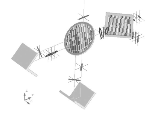
Figure 1: Schematic view of the Martin-Puplett interferometer.

The incoming polarized radiation passes through the wire-grid, is splitted in its two orthogonal components and after the roof-mirror reflection is phase-shifted to $\pi/2$ so that the transmitted radiation is now reflected and vice versa.
We can write the ideal Martin-Puplett interferometer Mueller matrix as following:

$$M_{MP}=\left(\begin{array}[]{cccc}1&0&0&0\\ 0&\cos(\delta)&0&\sin(\delta)\\ 0&0&-1&0\\ 0&\sin(\delta)&0&-\cos(\delta)\end{array}\right)$$ (1)

where $\delta$ represents the roof mirror phase-shift.

3.1 Cryostat

The MITOPol cryostat is composed by two tanks, one for nitrogen (2.5 l) and one for the ⁴He (2.8 l), and a ³He fridge; the working temperature is approximately 300 mK with a duration of cooling cycle of approximately 18 hours. Inside the cryostat, in thermal contact with cryogenic stages, a filter chain is mounted as shown in Fig. 2.

$\bf{Filters}$	$\bf{Cut-off/Cut-on(cm^{-1})}$	$\bf{Temperature(K)}$
Quartz	Low-pass (100)	300
Quartz + black poly	Low-pass (400)	77
Yoshinaga	Low-pass (55)	1,6
Mesh	Low-pass (14)	1,6
Yoshinaga	Low-pass (50)	0,3
Mesh	Low-pass (12)	0,3
Winston cone	High-pass (4)	0,3

Table 1: MITOPol filters chain with the relative working temperatures. The final band is 4-12 $cm^{-1}$.

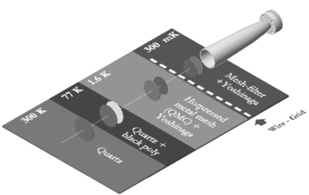
Figure 2: MITOPol filter chain.

A wire-grid splits the light in two beams collected by the f/3.5 Winston cones and absorved by two bolometers. The presence of two channels, operating at the same frequencies, allows a more efficient offset and noise removal. The incident signal on the detectors can be represented in the following way:

$$I_{1,2}=I_{0}\pm(Q*f(w,\delta,t)+U*g(w,\delta,t))\mp V\sin\delta$$ (2)

where $I_{0}$,$Q$,$U$,$V$ are the Stokes parameters, $\delta$ is the roof mirror phase-shift and $f$,$g$ are two periodic functions that depend from the chosen modulation system.
Observing the difference of the two outputs, normalized for the sum, we can detect the polarized signal embedded in the strong unpolarized one. The bolometers used in this experiment are spider-web bolometers developed at the University of Cardiff [19]. We use differential elettronic read-out in order to reduce DC components, microphonic noise and correlation between channels; we use 2 JFET to common drain, mounted on the ⁴He stage heated at a temperature of 120 K. Experimentally a value of $\sim 3nV/\sqrt{Hz}$ has been measured, optimal for the high sensibility demanded. The incident background (in the best atmospheric conditions) on the bolometers is of 500 pW, considering all the transmission curves of the filters; therefore the bolometer thermal conductivity has been chosen of the order of 10${}^{-9}W/K$.

4 Modulation System

The modulating element is fundamental in an experiment that aims to measure the polarized part of a signal, in fact it can alter the stage of the polarized signal, while leaving the unpolarized unaltered allowing to separate the polarized light from the unpolarized part of it.
In the following we will consider two possible modulation systems.

4.1 The Fresnel Double Rhomb

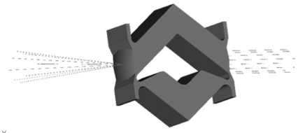
Figure 3: Simulation of $FDR$

$FDR$ is an optical element obtained by single polyethylene HDPE (High Density Poly-Ethylene) block constituted by two rhomboidal base prisms with an angle of $106^{o}.6$ between them. This object is based on the internal total reflection. The internal walls of the $FDR$ are tilted to $53^{o}.3$ with respect to the optic axis of the system, therefore the incident light on them will be totally reflected since the critical angle of total internal reflection for the passage from polyethylene to air is $41^{o}.14$. The radiation inside the $FDR$ undergoes four reflection on its walls. Using the Fresnel’s equations, it is possible to calculate, in case of total internal reflection, the phase-shift induced by a single reflection in this dielectric:

$$\delta=\phi_{s}-\phi_{p}=2\arctan\frac{\cos\vartheta_{1}\sqrt{\sin^{2}\vartheta_{1}-(1/n)^{2}}}{\sin^{2}\vartheta_{1}}$$ (3)

where $n$ is the HDPE refraction index.
From this equation, in order to obtain a phase-shift of $\pi/4$ we obtain two angles:

$$\vartheta_{1}=47^{o}.58$$ (4)

$$\vartheta_{1}^{{}^{\prime}}=55^{o}.37$$ (5)

The $FDR$ input (spherical shape with a curvature radius of 69 mm) is placed in the MITO f/4 focal plane [17] (the output has the same shape for simmetry) so inside the $FDR$ the beam is f/8.8. Using ray-tracing simulations we have obtained a distribution of phases-shifts centered around the value $\pi/4$ for an angle of $53^{o}.3$.
To modulate the polarization, we rotate the $FDR$ at a set frequency ($\omega$). Using Stokes formalism, the ideal $FDR$ Mueller Matrix becomes:

$$\mbox{{M}}_{DR}=\left(\begin{array}[]{cccc}1&0&0&0\\ 0&\cos 4\omega t&\sin 4\omega t&0\\ 0&\sin 4\omega t&-\cos 4\omega t&0\\ 0&0&0&-1\end{array}\right)$$ (6)

Therefore $Q$ parameter is modulated with a frequency 4 times the mechanical one, since bolometers are only sensitive to the intensity of the light, we add a wire-grid at the output of the $FDR$ to analyze the polarization of radiation; on the contrary the unpolarized radiation passes through unchanged.
The advantages of the $FDR$ with respect to the other modulation techniques are multiple: first of all the total reflection is not dispersive, so has a wide spectrum application; the total internal reflection does not attenuate the signal but it produces a phase-shift in the 4 reflections. Finally the polarization is modulated at a double frequency compared to the mechanic one allowing an efficient removal of microphonic noise connected to the measures.

4.1.1 Efficiency tests

Figure 4: Slow modulation data from measurements with two different setup: in the first (top-left panel) a fluorogold filter (with a cut-off about 30 $cm^{-1}$) is used. In the second (bottom-left) we reduced the band by means of a low-pass Mesh filter with cut-off to 10 $cm^{-1}$ in series with the fluorogold filter. In each of these plots, two curves are presented, one with parallel wire-grids and a second one with wire-grids orthogonal with each other. The right diagram represents the ratio of the two spectra measured at two maximum positions in the slow modulation configuration with parallel and orthogonal wire-grids using only the fluorogold filter. The efficiency in our band is $19\pm 5$%.

Efficiency tests have been performed illuminating the $FDR$ with a polarized radiation and detecting it as it gets modified by th $FDR$ itself. The tests are realized by using a Hg lamp as a source. The lamp emits in all the electromagnetic spectral range and in the millimetric its emission is similar to a black body at a temperature between 3000 K and 3500 K. Moreover a Lamellar Grating interferometer [18] has been used to measure the spectral behaviour of the $FDR$.
Several interferograms have been realized with 256 mechanical steps of 80 $\mu m$ each one. The frequency band-width can be investigated in a range between 3-31.25 $cm^{-1}$.
A lab. cryostat has been used for laboratory tests using a bolometer working at 1.6 K temperature.
We set the outgoing beam from the Lamellar Grating as an f/4, since it must reproduce as faithfully as possible the working conditions of the instrument.

In order to study its polarization efficiency, we have used two wire-grids: the first one located in front of $FDR$ and the second one behind it. In this situation the radiation that enters into the $FDR$ is completely polarized in the orthogonal direction respect to the wires of the wire-grid; into the $FDR$ the radiation is phase-shifted, and then the second wire-grid allows to analyze the modulated contribution of polarization. If the $FDR$ rotates at a frequency about 2 mHz, a modulation is observed at a frequency 4 times the mechanical one. Ideally, if we perform two different measurements one with parallel wire-grids and the second one with orthogonal wire-grids with each other, we should observe the same amplitude in both signals with a phase-shift of $\pi/2$. Then we made two interferograms stopping the $FDR$ in two positions corresponding to the maximum of modulation in the parallel and orthogonal wire-grids setups. The expected result is a constant spectrum with unity value. Fig. LABEL:fig:Fig_5 evidences a loss of efficiency in the centre of our band-width; this corresponds to an efficiency of phase-difference in the band 4-12 $cm^{-1}$ of $19\pm 5$%.
To explain this inefficiencies different motivations have been proposed and investigated: diffractional effects could change the beam f/#. Gaussian Optic simulation have been shown that inside the $FDR$ the effect is negligible. In any case we would expect a global decrease of the efficiency at low frequencies which is not observed in our data.
The possibility for a radiation beam to go through the structure housing the $FDR$ without entering the $FDR$ itself has been ruled out by several measuraments without the external structure and shielding with aluminium and Eccosorb all the possible leaks.
Tests have also been performed using a more collimated beam with respect to the f/# that the $FDR$ would see at the telescopes focal plane showing the same results as in previous case.
The possibility that the polyethylene (the one we have used) has a varying refraction index with the frequency has been investigated by measuring it in the already cited frequency bands. We have used, as source, Eccosorb at 77 K and 300 K modulated at a frequency of 12 Hz and as interferometer the $MPI$.
This measurement has been performed by placing a polyethylene sample in one of the arms of $MPI$ and measuring the distance between the zero path difference position obtained with and without the sample itself. This has allowed to measure the optical path delay introduced by polyethylene and, known the sample thickness, one can derive the refraction index.
The difference is equal to:

$$\Delta^{ZPD}_{Opt}=d(n-1)$$ (7)

Where $\Delta^{ZPD}_{Opt}$ is the optical shift, $d$ is the polyethylene sample thickness and $n$ is the polyethylene refraction index.
This measurement realized using band-pass filters inside our spectral range, has confirmed refraction index value reported in lecterature. The integrated value inside the band is:

$$n=1.5276\pm 0.0066$$ (8)

Figure 5: Slow modulation with the same setup of Fig. 4 using the Mesh filter with cut at 10 $cm^{-1}$ and the fluorogold filter in series: the improvement is evident.

Figure 6: Spectrum obtained with the same setup of Fig. 4: the loss of efficiency towards greater frequencies. In this case the phase-shift efficiency is increased to $86\pm 8$%.

A further possibility is that our $FDR$ could be affected by optical activity since, at manufacturing stage, it has undergone stresses and thermal shocks [20, 21]. The optical activity produces, in analogy to the birifrangent materials, an induced polarization [22]. It depends by the molecule simmetry that constitutes the substance and by the degree of disorder that is inside the lattice. All the molecules of organic nature or synthetize by living organism, are optical active. The structure of the polyethylene is constituted with a carbon chain where every atom is tied to two hydrogen atoms; if the chain is linear it is defined high density polyethylene (HDPE). These chains can be very long assuming macroscopic dimension and therefore comparable with the wavelengths that we investigate. As a result, we could see anisotropies and spurious polarization effects varying with the frequency. This effect has been tested by heating the $FDR$ at temperatures just below the HDPE melting point (137 $C$) in order to let the internal structure relax and acquire again the isotropic structure needed for an optical element to be used in polarization measurements. The $FDR$ has been gradually heated and finally left at 135 $C$ for 48 hours and at 137 $C$ for 12 hours.
After these thermal cycles we have repeated the same measurements in order to compare the results which are shown in Fig. 5 and Fig. 6.
The $FDR$ efficiency is considerably increased ($86\pm 8$%).

4.2 Phase modulation with Martin-Puplett interferometer

Using $MPI$ is an alternative method to modulate the polarization, both as an interferometer and as a phase modulator [23, 24]. The basic idea is to wobble one of the two roof mirrors along the optical axis. In order to write the $MPI$ Mueller matrix one needs to consider eq. 1 and to substitute $\delta\rightarrow\delta^{{}^{\prime}}=\delta-\delta_{m}$, where $\delta=2\pi\Delta x_{opt}/\lambda$ and $\delta_{m}=2\pi f(\omega,t)/\lambda$.
The optical path difference $\delta^{{}^{\prime}}$ represents the modulation term. The function f($\omega$,t) represents the roof mirror wave form. The new Martin-Puplett Mueller matrix becomes:

$$M_{MP}^{New}=\left(\begin{array}[]{cccc}1&0&0&0\\ 0&\cos(\delta^{{}^{\prime}})&0&\sin(\delta^{{}^{\prime}})\\ 0&0&-1&0\\ 0&\sin(\delta^{{}^{\prime}})&0&-\cos(\delta^{{}^{\prime}})\end{array}\right)$$ (9)

From eq. 9 we can note that the polarizated radiation is modulated while the unpolarized radiation remains unchanged; however the polarization plane is not rotated. The effect of the modulation is independent from the choice of the oscillating roof mirror; the practical solution that we adopted has been of oscillating the roof mirror each step.
Using a lock-in amplifier, the output is proportional to the interferogram derivative. The smaller is the amplitude the more the signal approximates to punctual derivative but with a decreasing intensity. Nevertheless one needs to consider that the radiation wavelength is in the range between 850 $\mu m$ and 2.5 $mm$ so, in order to be efficiently modulated, it is not possible to choose an amplitude modulation much smaller than the wavelength of interest. On the other side, important spectral information can be lost if we modulate with an amplitude higher than the step; as a matter of fact using a great amplitude could be possible to modulate among two points with similar intensity, smoothing therefore the interferogram. An optimal choice for the amplitude modulation is to set it equal to the modulation step.

Figure 7: Simulated signal obtained with phase modulation .

The relation that links Fourier transform of interferogram to its derivative is:

$$FT[f^{{}^{\prime}}(x)](k)=C_{o}\cdot|2J_{1}(2\pi kA/2)|\cdot FT[f(x)](k)$$ (10)

where in the case of phase-modulation $C_{o}$ is the term of Fourier series, A is the modulation amplitude and $J_{1}$ is the Bessel first kind and order 1 function.

From eq. 10 we note that the result is always lower than 1, compared with “classical” modulation; then, to maximize the signal, it is worth to choose the wave form in order to have the maximum $C_{o}$. The wave square modulation is the best with $C_{square}=4/\pi$.
One of the classical spectroscopy problems, particularly at high resolution, is the difficult to recognize between small variations due to the source and variations due to other factors; in fact a small variation on the interferogram, due for example to atmospheric fluctuations, affects heavily the spectrum, and produces signal variations that may be confused with emission or absorption lines [25].
Using the phase modulation this problem has been solved; in this case, the baseline of the interferogram is about zero, see Fig. 7; instead the baseline of the classical modulation is $I(0)/2$ [26]; and so any signal originated by a fluctuation (instantaneous) is near to the zero level of the interferogram and does not affect the spectrum.
Another advantage of phase modulation, is observation time; in fact with phase modulation we observe constantly the source. Moreover [23, 27], the signal to noise ratio is $\frac{(S/N)_{PM}}{(S/N)_{AM}}=4\mid J_{1}(2\pi\nu\frac{A}{2})\mid$, and so when the Bessel function is greater than 0.25 the signal to noise ratio, in the phase modulation (PM), is greater than the amplitude modulation (AM) [28]. The spectrum obtained with the phase modulation is divided by Bessel function (first kind and order 1) thus, when this function is equal to zero, we have a loss of informations. While the amplitude modulation is small there are no problems; when the amplitude modulation is high, this zero value could be on the frequency range that we are studying. The loss of information, choosing amplitude modulation equal to the interferogram step, is out of our range.

4.2.1 Measurement

We have mounted this experiment at focal plane of MITO telescope [29], we have obtained spectra on atmospherics emission in the range 4-12 $cm^{-1}$, placing the wire-grid in front of the interferometer polarizing all the incident radiation.
In Fig. 8 we have reported the interferograms operating on the atmosphere emission, obtained with an elevation equal to $60^{o}$ with step and amplitude modulation equal to 100 $\mu m$.

Figure 8: Interferogram obtained at $60^{o}$ of elevation (the two signals are overlapped); we note the good correlation between the two channels.

From these interferograms we have obtained the spectrum, shown in Fig. 9 and we have compared it with simulated emission with ATM program [30, 31, 32, 33].

Figure 9: Atmospheric emission at MITO (subracted by a Black Body source at 77K as reference source), measured with two channel of the polarimeter. The outlined line is an atmospheric emission simulated with pwc 2.3 mm. It is clear the loss of spectral resolution at frequencies corresponding to $H_{2}O$ and $O_{2}$ emission

We have performed polarimetric measurements removing the wire-grid in front of Martin-Puplett interferometer; any excess of polarization obtained from this interferograms is an indicator of the spurious polarization of the instrument, see Fig. 10, considering that the atmosphere emission at this wavelength is not expected to be polarized [7].

Figure 10: Instrumental spurious polarization in one direction (Telescope + Polarimeter).

From the Fig. 10 we obtain a value of the spurious polarization in one direction lower than 1%.

5 Conclusions

In this paper we have presented two polarization modulation methods. The first method have evidenced that the optical activity of the polyethylene realized by a not homogeneous block can alter the entering polarization; on the other side this amplitude modulation method is independent by the wavelength of the radiation.
The phase modulation gains observation time and does not present a decrease by transmission. However the polarization plane is not rotate so we have to insert a optic element that produces a polarization rotation after the interferometer.

An introduction to the Stokes parameters

A plane electromagnetic wave with its Poynting vector directed along the z axis can be decomposed into its two components in the x and y direction: $E_{x}(z,t)$ and $E_{y}(z,t)$. If any correl ation between two vectors exists, the plane wave will be defined polarized.
In order to obtain observable quantities, we always have to consider the temporal average of the polarization ellipse. However the temporal process of average can be avoided representing the real optical amplitudes in terms of complex amplitudes:

$$I = E_{x}E_{x}^{*}+E_{y}E_{y}^{*}$$

$$Q = E_{x}E_{x}^{*}-E_{y}E_{y}^{*}$$

$$U = E_{x}E_{y}^{*}+E_{y}E_{x}^{*}$$ (11)

$$V = E_{x}E_{y}^{*}-E_{y}E_{x}^{*}$$

These quantities are called Stokes parameters; Q and U depend, for construction, on the chosen coordinates system.
I represents the intensity of the e-m wave considered.
Q represents the contribution of the linear polarization horizontal and vertical.
U describes the contribution of linear polarization at an angle of $\pm 45$.
V describes the contribution of circular polarization towards right and left.
The Stokes parameters are real quantities, they are observable and the following expression is always true:

$$I^{2}\geq Q^{2}+U^{2}+V^{2}$$ (12)

where the equal is used for fully polarized light. It is possible to define a Stokes vector whose 4 parameters are the elements of a column vector.

$${\mathcal{S}}=\left(\begin{array}[]{ccc}I\\ Q\\ U\\ V\end{array}\right)$$ (13)

The Stokes parameters describe the wave polarization degree; this can be evidenced defining the quantity:

$$P\equiv\frac{I_{pol}}{I}=\frac{\sqrt{Q^{2}+U^{2}+V^{2}}}{I},\ 0\leq P\leq 1$$ (14)

When a beam crosses an element that can change its polarization state, the elements of the Stokes vector will vary depending on the particular considered element.
We consider an incoming beam defined by whichever Stokes vector; the outgoing beam from the element will be characterized by a vector $S_{i}^{{}^{\prime}}=(I^{{}^{\prime}},Q^{{}^{\prime}},U^{{}^{\prime}},V^{{}^{\prime}})$ where

$$I^{{}^{\prime}} = m_{00}I+m_{01}Q+m_{02}U+m_{03}V$$

$$Q^{{}^{\prime}} = m_{10}I+m_{11}Q+m_{12}U+m_{13}V$$

$$U^{{}^{\prime}} = m_{20}I+m_{21}Q+m_{22}U+m_{23}V$$ (15)

$$V^{{}^{\prime}} = m_{30}I+m_{31}Q+m_{32}U+m_{33}V$$

therefore the following equation can be written:

$$S^{{}^{\prime}}=M\cdot S$$ (16)

M is the Mueller matrix of the optical element. The electric field vector of a e-m wave can be changed in its amplitude,phase or direction and this change is described by the matrix M.
The terms in a Mueller matrix have different meanings: the terms found in the trace define the transmission and the depolarization of the element. The terms $m_{01},m_{02},m_{03},m_{10},m_{20},m_{30}$ contain the contribution of spurius polarization of the element. The remaining terms contain the passage of the light from Q to U or V polarization.
On the contrary the inverse is not valid, as it is not possible to identify a coefficient by a single effect [34, 35].

References

- [1] C.Ceccarelli et al. The Polarization of the Cosmic Background an the universal magnetic field. Proceedings of the Seventeenth Moriond Astrophysics Meeting, A84:191–203, 1982.
- [2] N.Caderni et al. Polarization of the Microwave Background Radiation I-Anisotropic cosmological expansion and evolution of the polarization states. Physical Rev.D, 17:1901–1907, 1978.
- [3] A.Kosowsky. Introduction to Cosmic Microwave Background. New Astron.Rev., 43:157, 1999.
- [4] W.Hu e M.White. A CMB Polarization Primer. New Astron., 2:323, 1997.
- [5] N.Caderni et al. Polarization of the Microwave Background radiation II-an infrared survey of the sky. Physical Rev.D, 17:1908–1918, 1978.
- [6] A.Blanco et al. Polarization of the Cosmic Background Radiation - an experimental approach. Marcel Grossmann Meeting: General Relativity, 2D:919, 1982.
- [7] S.Hanany P.Rosenkranz. Polarization of the atmosphere as a Foreground for Cosmic Background Polarization experiments. New Astron.Rev, 2003.
- [8] Angelica de Olivera-Costa et al. The Large-Scale Polarization of the Microwave Foreground. Phys.Rev, D:68, 2003.
- [9] A.Kogut et al. Wilkinson Microwave Anisotropy Probe (WMAP) First Year Observations: TE Polarization. ApJ.Suppl., 148:161, 2003.
- [10] J.Kovac et al. Detection of Polarization in the Cosmic Microwave Background Using DASI. Nature, 420:772–787, 2002.
- [11] E.M.Leitch. Measuring Polarization with DASI. Nature, 420:763–771, 2002.
- [12] E.S.Battistelli et al. Far Infrared Polarimeter with Very Low Instrumetal Polarization. SPIE conference proceedings:Astronomical telescopes and instrumentation, 4843,241-249, 2003.
- [13] G.Pisano. Millimiter CBR polarimetry: the POLCBR experiment at MITO. New Astr.Rev, 43:329–339, 1999.
- [14] G.Pisano. Realizzazione e Calibrazione di un Polarimetro per misure della Radiazione di Fondo Cosmico nel lontano infrarosso. PHD Thesis in Astronomy XII course, University of Rome ’La Sapienza’, 2004.
- [15] D.K.Lambert P.L.Richards. Martin-Puplett interferometer: an analysys. Infrared Physics, 17:1595, 1978.
- [16] D.H.Martin E.Puplett. Polarised interferometric spectrometry for the millimetre and submillimetre spectrum. Appl.Opt., 10:105, 1969.
- [17] M. De Petris et al. A ground based experiment for CMBR anisotropy observations: MITO. New Astron.Rev., 43:297–315, 1999.
- [18] R.J.Bell. Introductory Fourier Trasform Spectroscopy. Academic Press, 1972.
- [19] A.Orlando. Optimization and realization of bolometric detectors for high sensitivity measurements of the Cosmic Microwave Background. PHD Thesis in Astronomy XVI course, University of Rome ’La Sapienza’, 2004.
- [20] G.A.Ediss and D.Koller. 68.5 to 118 GHz measurament of possible infrared filter materials: black polyethylene,zitex and grooved and un-grooved fluorogold and HDPE. ALMA MEMO, N412, 2002.
- [21] G.A.Ediss and T.Globus. 60 to 450 GHz trasmission and reflection measuraments of gooved and un-grooved HDPE plates. ALMA MEMO, N347, 2001.
- [22] C.Cantor and P.Schimmel. Biophysical Chemistry. W.H.Freeman, 1980.
- [23] J.Chamberlain. Phase modulation in far infrared (submillimetre-wave) interferometers. I-Mathematical Formulation. Infrared Physics, 11:25–55, 1971.
- [24] J.Chamberlain H.A.Gebbie. Phase modulation in far infrared (submillimetre-wave) interferometers. II-Fourier Spectrometry and Terametrology. Infrared Physics, 11:57–73, 1971.
- [25] P.Connes J.P.Maillard and J.Connes. Spectroscopie astronomique par transformation de Fourier. Journal de Physique, Colloque C2, Tome 28, pp.120-135, 1967.
- [26] L.Mertz. Spectrom tre stellaire multicanal. Journal de Physique et le radium, Tome 19, pp.233-236, 1958.
- [27] J.Chamberlain M.J.Hine, J.Haigh. Phase modulation in far infrared (submillimetre-wave) interferometers. III-Laser Refractometry. Infrared Physics, 11:75–84, 1971.
- [28] J.E. Harries and P.A.R. Ade. The high resolution millimetre wavelength spectrum of the atmosphere. Infrared Physics, 12:81–94, 1972.
- [29] M. De Petris et al. MITO: the 2.6 m millimeter telescope at Testa Grigia. New Astron.Rev., 1:121, 1996.
- [30] Michel Guelin. Atmospheric Absorption. Proceedings of the workshop on the IRAM Millimeter Interferometry Summer School, 1998.
- [31] E.Eerabin et al. Submillimeter FTS Measurements of Atmospheric Opacity above Mauna Kea. Appl.Opt., 37:2185–2198, 1998.
- [32] J. R. Pardo E. Serabyn, J. Cernicharo. Atmospheric Transmission at Microwaves (ATM): An Improved Model for mm/submm applications. IEEE Trans. on Antennas and Propagation, 49/12, 1683-1694, 2001.
- [33] J.R.Pardo-Carrion. Etudes de l’atmosphère terrestre au moyen d’observations dans les longueurs d’onde millimetriques et submillimetriques. Doctorat Europeen Universite Paris VI - Universidad Complutense de Madrid, 1996.
- [34] E.Collett. Polarized Light. Marcel, 1993.
- [35] S.Huard. Polarization of Light. J.Wiley and Sons, 1997.