A new multidimensional AMR Hydro+Gravity Cosmological code

Abstract

A new cosmological multidimensional hydrodynamic and N-body code based on an Adaptive Mesh Refinement scheme is described and tested. The hydro part is based on modern high-resolution shock-capturing techniques, whereas N-body approach is based on the Particle Mesh method. The code has been specifically designed for cosmological applications. Tests including shocks, strong gradients, and gravity have been considered. A cosmological test based on Santa Barbara cluster is also presented. The usefulness of the code is discussed. In particular, this powerful tool is expected to be appropriate to describe the evolution of the hot gas component located inside asymmetric cosmological structures.

1 Introduction

Numerical simulations of structure formation are essential tools in theoretical cosmology. Their main role, in addition to many other uses, has been to test the viability of the different models of structure formation – e.g. variants of the cold dark matter (CDM) model – by evolving initial conditions using basic physical laws.

Historically, the use of cosmological simulations started in 1960s (Aarseth 1963) and 1970s (e.g. Peebles 1970, White 1976). These calculations were N-body, collisionless, simulations with few particles. In early 1980s, the N-body techniques and computers advanced to the extent that simulations could be applied systematically as a scientific tool ( see Hockney & Eastwood 1988 for a good review of N-body techniques) and their use led to important results such as the development of the CDM paradigm (Peebles 1982, Blumenthal et al. 1984, Davies et al. 1985). N-body techniques have continued to be developed and refined, with examples including AP3M (Couchman 1991), ART code (Kravtsov, Klypin & Khokhlov 1997), GADGET code (Springel, Yoshida & White 2001), MLAPM (Knebe, Andrew & Binney 2001) or more recently the code presented by Bode & Ostriker (2003).

The physics of the gaseous, baryonic, component of the Universe is far more complicated to model than the formation of structures in the dark matter due to gravitational instability. Understanding the behaviour of baryons is crucial for a complete theory of the formation of cosmic structures, particularly on galactic and cluster scales. Any realistic simulation which sets out to explain the growth of structures in the Universe must therefore contain a hydrodynamical treatment of the evolution of the baryonic fluid. Pioneering simulations using Smooth Particle Hydrodynamics (SPH) techniques were first carried out by Gingold & Monaghan (1977); early cosmological simulations that followed baryons and dark matter include those by Evrard (1988) and Hernquist & Katz (1989).

The integration of the hydrodynamics equations governing the evolution of gas can be done using different techniques. The adoption of a particular technique, with its associated benefits and drawbacks, has a direct consequence on the outcome of the simulation. The numerical techniques used to model the evolution of the baryons can be split into two general classes: Lagrangian and Eulerian.

The most popular of the Lagrangian scheme is SPH(Lucy 1977, Gingold & Monaghan 1977). Other schemes which could be defined as quasi-Lagrangian include those described by Gnedin (1995) and Pen (1995). SPH techniques have made possible huge advances in the field of numerical Cosmology in the recent past. Relatively easy to implement and with a low computational cost, SPH techniques have a huge dynamical range because of their Lagrangian nature. This feature has made them particularly successful in simulations of cosmic structure formation. However, the SPH technique also has significant drawbacks, including (i) an approximate treatment and description of shock waves and strong gradients, (ii) a poor description of low density regions, (iii) a requirement to the use of numerical artifacts such as the artificial viscosity and (iv) the possible violation of conservation properties (see Okamoto et al. (2003) for a recent example of unphysical results in simulations due to the SPH nature).

Eulerian schemes present an alternative to Lagrangian schemes. Within this board class of techniques, the ones based on Riemann solvers have been particularly successful (e.g. Ryu et al. 1993; Quilis, Ibáñez & Sáez 1994; Bryan, Norman, Stone, Cen & Ostriker 1995; Gheller, Pantano & Moscardini 1998, and others). These numerical schemes are written in conservative form, which ensures excellent conservation of physical quantities. Shock waves, discontinuities and strong gradients are sharply resolved in typically one or two cells. The use of Riemann solvers removes the need to invoke artificial viscosity to integrate equations with discontinuities. Although these properties are needed in order to build a robust hydrodynamical scheme, precisely due to their Eulerian character – fix numerical grids are needed to integrate the hydrodynamical equations – these techniques are limited by poor spatial resolution. In order to achieve adequate resolution, dense numerical grids are needed which quickly drives up the computational cost. Even with the best computers available nowadays, a simple Eulerian approach cannot compete with a Lagrangian approach in cosmological applications, which demand a good spatial resolution and a huge dynamical range.

In this paper, we present a new numerical code which combines the best features of the Eulerian and Lagrangian approaches. The basic idea is to improve the numerical resolution by implementing a scheme known as Adaptive Mesh Refinement (AMR) described originally by Berger & Oliger (1984) and Berger & Colella (1989). In order to do this, we use an Eulerian approach as the ones described above, but gaining resolution – both spatial and temporal – by selectively refining the original computational grid. The result is a hierarchy of nested grids which naturally behaves as a Lagrangian scheme (the grids are refined only where the calculation requires it) and each one of these grids is treated as an independent computational domain by the Eulerian scheme.

AMR schemes have proved to be extremely powerful in many fluid dynamics applications. In cosmology, recent AMR implementations have been designed by Bryan & Norman (1997), Kravtsov, Klypin & Hoffman (2002) and Teyssier (2002). These codes share the basic ingredients with the one described in this paper, although there are slight differences depending on each particular implementation.

The central tenet of the AMR scheme, the refinement of the computational grid wherever better resolution is needed, can be exploited to incorporate an N-body scheme to follow the evolution of dark matter. The Particle-Mesh(PM) method is ideally suited for grating onto an hydro-AMR code. In practise, a PM scheme is used for each nested grid, with progressively higher spatial resolution when the cell size gets smaller. This implementation of the AMR-PM has the advantage of avoiding the problem of setting a softening parameter in the gravitational force law, as this parameter is naturally determined by the cell size. Several implementations of this approach for dark matter only have been presented in the literature with different degrees of success (Villumsen 1989, Jessop et al. 1994; Splinter 1996; and Kravtsov, Klypin & Khokhlov 1997).

In the present paper, we describe a new coupled hydrodynamical and N-body code for cosmological applications – called MASCLET (Mesh Adaptive Scheme for CosmologicaL structurE evoluTion) – based on an AMR scheme. The basic hydrodynamical solver is based on the Piecewise Parabolic Method (Colella & Woodward 1984) whereas the N-body method used is a classic PM according to Hockney & Eastwood (1988). The scheme presented in this paper is able to refine and unrefine grids automatically according with a set of parameters which can be chosen depending upon the application. The code is written in Fortran 90 and there is a parallel version using OpenMP standard directives.

The following section is devoted to present the equations describing the evolution of gaseous and dark matter components, and the main features of the basic hydrodynamical and N-body schemes for a fix grid. Sec. 3 describes the AMR strategy and how it is implemented in the code. In Sec. 4, we present several numerical tests including the so-called Santa Barbara cluster (Frenk et al. 1999). Finally, our main conclusions are summarized in Sec. 5.

2 Equations and the basic numerical procedure

In this Section we write down the basic equations governing the evolution of cosmological inhomogeneities as a hyperbolic system of conservation laws. The mathematical properties of this kind of system and the numerical algorithms specifically designed for solving it have been well studied in the literature (LeVeque 1992, Toro 1997).

2.1 Gas dynamics

2.1.1 Evolution equations in conservation form

For spatial scales where relativistic corrections are not required, cosmological inhomogeneities evolve according to the following equations (Peebles 1980):

$$\frac{\partial\delta}{\partial t}+\frac{1}{a}\nabla\cdot(1+\delta){\bf v}=0$$ (1)

$$\frac{\partial{\bf v}}{\partial t}+\frac{1}{a}({\bf v}\,\cdot\,\nabla){\bf v}+H{\bf v}=-\frac{1}{\rho a}\nabla p-\frac{1}{a}\nabla\phi$$ (2)

$$\frac{\partial E}{\partial t}+{1\over a}\nabla\cdot[(E+p){\bf v}]=-3H(E+p)-H\rho{\bf v}^{2}-\frac{\rho{\bf v}}{a}\nabla\phi$$ (3)

$$\nabla^{2}\phi=\frac{3}{2}H^{2}a^{2}\delta$$ (4)

where ${\bf x}$, ${\bf v}=a(t)\frac{d{\bf x}}{dt}=(v_{x},v_{y},v_{z})$, and $\phi(t,{\bf x})$ are, respectively, the Eulerian coordinates, the peculiar velocity, and the peculiar Newtonian gravitational potential. The total energy density, $E=\rho\epsilon+{1\over 2}\rho v^{2}$ , is defined as the addition of the thermal energy, $\rho\epsilon$, where $\epsilon$ is the specific internal energy, and the kinetic energy (where $v^{2}=v_{x}^{2}+v_{y}^{2}+v_{z}^{2}$). The background parameters are the scale factor, $a$, background density, $\rho_{{}_{B}}$, and the Hubble constant, $H$. The density contrast , $\delta$, is defined as $\delta=\rho/\rho_{{}_{B}}-1$. Pressure gradients and gravitational forces are the responsible for the evolution.

Poisson’s equation (4) is an elliptic equation, and its solution depends on the boundary conditions. This equation has to be solved in conjunction with Eqs (1–3) to compute the source term $\nabla\phi$ which appears in Eqs (2–3).

An equation of state $p=p(\rho,\epsilon)$ closes the system. In this paper we used an ideal gas equation of state $p=(\gamma-1)\rho\epsilon$ with $\gamma=5/3$.

The hydrodynamic equations Eqs (1–3) can be rewritten in a slightly different form:

$$\frac{\partial{\bf u}}{\partial t}+\frac{\partial{\bf f(\bf u)}}{\partial x}+\frac{\partial{\bf g(\bf u)}}{\partial y}+\frac{\partial{\bf h(\bf u)}}{\partial z}={\bf s(\bf u)}$$ (5)

where ${\bf u}$ is the vector of unknowns(conserved variables):

$${\bf u}=[\delta,m_{x},m_{y},m_{z},E]\ \ ,$$ (6)

the three flux functions ${\bf F}^{\alpha}\equiv\{{\bf f},{\bf g},{\bf h}\}$ in the spatial directions $x,y,z$, respectively , are defined by

$${\bf f(\bf u)} = \left[\frac{m_{x}}{a},\frac{m_{x}^{2}}{(\delta+1)a}+\frac{p}{a\rho_{{}_{B}}},\right.$$ (7)

$$\left.\frac{m_{x}m_{y}}{(\delta+1)a},\frac{m_{x}m_{z}}{(\delta+1)a},\frac{(E+p)m_{x}}{a(\delta+1)}\right]$$

$${\bf g(\bf u)} = \left[\frac{m_{y}}{a},\frac{m_{x}m_{y}}{(\delta+1)a},\right.$$ (8)

$$\left.\frac{m_{y}^{2}}{(\delta+1)a}+\frac{p}{a\rho_{{}_{B}}},\frac{m_{y}m_{z}}{(\delta+1)a},\frac{(E+p)m_{y}}{a(\delta+1)}\right]$$

$${\bf h(\bf u)} = \left[\frac{m_{z}}{a},\frac{m_{x}m_{z}}{(\delta+1)a},\right.$$ (9)

$$\left.\frac{m_{y}m_{z}}{(\delta+1)a},\frac{m_{z}^{2}}{(\delta+1)a}+\frac{p}{a\rho_{{}_{B}}},\frac{(E+p)m_{z}}{a(\delta+1)}\right]$$

and the sources ${\bf s}$ are

$${\bf s(\bf u)} = \left[0,-\frac{(\delta+1)}{a}\frac{\partial\phi}{\partial x}-Hm_{x},\right.$$ (10)

$$- \frac{(\delta+1)}{a}\frac{\partial\phi}{\partial y}-Hm_{y},-\frac{(\delta+1)}{a}\frac{\partial\phi}{\partial z}-Hm_{z},$$

$$- 3H(E+p)-\frac{\rho_{{}_{B}}Hm^{2}}{(\delta+1)}-\frac{m_{x}\rho_{{}_{B}}}{a}\frac{\partial\phi}{\partial x}-\frac{m_{y}\rho_{{}_{B}}}{a}\frac{\partial\phi}{\partial y}$$

$$- \left.\frac{m_{z}\rho_{{}_{B}}}{a}\frac{\partial\phi}{\partial z}\right]$$

where $m_{x}=(\delta+1)v_{x}$, $m_{y}=(\delta+1)v_{y}$, and $m_{z}=(\delta+1)v_{z}$.

System (5) is a three-dimensional hyperbolic system of conservation laws with sources ${\bf s}({\bf u})$. From the numerical point of view is important to introduce the Jacobian matrices associated to the fluxes:

$${\bf\cal A}^{\alpha}=\frac{\partial{\bf F}^{\alpha}({\bf u})}{\partial{\bf u}}$$ (11)

Hyperbolicity demands that any real linear combination of the Jacobian matrices $\xi_{\alpha}{\bf\cal A}^{\alpha}$ should be diagonalizable with real eigenvalues (LeVeque 1992). This is of crucial importance from the numerical point of view.

The spectral decompositions of the above Jacobian matrices in each direction, i.e., the eigenvalues and eigenvectors are explicitly written in Quilis, Ibáñez & Sáez (1996).

The sources do not contain any term with differential operators acting on hydrodynamical variables ${\bf u}$. This is an important property consistent with the fact that the left hand side of Eq. (5) defines a hyperbolic system of conservation laws.

2.2 The hydro code

The mathematical properties resulting from the hyperbolic character of the system of equations (5) allow us to design a set of numerical techniques known as high-resolution shock-capturing (HRSC). These techniques are the modern implementation of Godunov’s original method (Godunov 1959, see Laney (1998) for a modern review on Godunov schemes and Eulerian methods).

The HRSC techniques have several key ingredients such as the reconstruction procedure, the Riemann solver, and time advancing schemes which can vary in different implementations. Nevertheless, all of these implementations share the same basic properties: the ability to handle shocks, discontinuities and strong gradients in the integrated quantities, and excellent conservation properties.

Our basic hydro solver is based on a particular implementation of the HRSC methods – see Quilis, Ibáñez & Sáez (1996) for more details. The main ingredients of our solver are the following:

1. It is written in conservation form. This is a very important property for a numerical algorithm designed to solve, numerically, a hyperbolic system of conservation laws. That is, in the absence of sources, those quantities that ought to be conserved –according to the differential equations– are exactly conserved in the difference form.

2. Reconstruction procedure. This procedure allows the method to gain resolution by reconstructing, through interpolations, the distribution of the quantities within the numerical cells. In order to increase spatial accuracy, we have used two cell-reconstruction techniques. We have implemented a linear reconstruction – first order –, with the minmod function (Quilis, Ibáñez & Sáez 1994) as a slope limiter. With this reconstruction, our algorithm is a MUSCL-version (van Leer 1979) and second order accurate in space. We have also implemented a parabolic reconstruction (PPM) subroutine according to the procedure derived by Colella & Woodward (1984). With the parabolic reconstruction, the algorithm is third order accurate in space. Statements on the order of the scheme must be taken with caution, as the mathematical proofs only exist for the one-dimensional case, being the order reduced in multidimensional extensions. In any case, the higher the order of the method in 1D, the better the accuracy in the multidimensional applications.

   Hence, from the cell-averaged quantities ${\bf u}_{i,j,k}$ we construct, in each direction, a piecewise linear or parabolic function which preserves monotonicity. Thus, the quantities, ${\bf u}_{i+{1\over 2},j,k}^{R},{\bf u}_{i,j+{1\over 2},k}^{R},{\bf u}_{i,j,k+{1\over 2}}^{R}$ and ${\bf u}_{i+{1\over 2},j,k}^{L},{\bf u}_{i,j+{1\over 2},k}^{L},{\bf u}_{i,j,k+{1\over 2}}^{L}$, can be computed; the superindices $R$ and $L$ stand for the values at both sides of a given interface between neighbour cells. These values at each side of a given interface allow us to define the local Riemann problems. The numerical fluxes can be computed through the solution of these local Riemann problems.

3. Numerical fluxes at interfaces. We have used a linearized Riemann solver following an approach similar to the one described by Roe (1981). The procedure, applied in each direction, starts by constructing the corresponding numerical flux according to Roe’s prescription and in order to do that it is necessary to know the spectral decomposition of the Jacobian matrix ${\cal A}^{\alpha}$. The numerical flux associated with the $x$-direction is:

   $${\widehat{{\bf f}}}_{i+{1\over 2},j,k}=\frac{1}{2}\left(\frac{}{}\right.{\bf f}({\bf u}_{i+{1\over 2},j,k}^{L}) + {\bf f}({\bf u}_{i+{1\over 2},j,k}^{R})$$ (12)

   $$- \left.\sum_{{\eta}=1}^{5}\mid\widetilde{\lambda}_{\eta}^{x}\mid\Delta\widetilde{\omega}_{\eta}{\widetilde{\bf R}}^{x}_{\eta}\right)$$

   where ${\widetilde{\lambda}}_{\eta}^{x}$ and ${\widetilde{\bf R}}_{\eta}^{x}$ ($\eta=1,2,3,4,5$) are, respectively, the eigenvalues and the $\eta$-right eigenvector of the Jacobian matrix:

   $${\cal A}^{x}{\rm{}_{i+{1\over 2},j,k}}=\left(\frac{\partial\bf f(\bf u)\rm}{\partial\bf u\rm}\right)_{{\bf u}=({\bf u}_{i+{1\over 2},j,k}^{L}+{\bf u}_{i+{1\over 2},j,k}^{R})/2}.$$ (13)

   These are calculated in the state which corresponds to the arithmetic mean of the states at each side of the interface. The quantities $\Delta\widetilde{\omega}_{\eta}$ – the jumps in the local characteristic variables through each interface– are obtained from the following relation

   $${\bf u}^{R}-{\bf u}^{L}=\sum_{\eta=1}^{5}\Delta\widetilde{\omega}_{\eta}{\widetilde{\bf R}}_{\eta}^{x}$$ (14)

   where $\widetilde{\lambda}_{\eta}^{x}$, $\widetilde{\bf R}_{\eta}$ and $\Delta\widetilde{\omega}_{\eta}$, are functions of $\bf u$, which are calculated at each interface and, consequently, they depend on the particular values ${\bf u}^{L}$ and ${\bf u}^{R}$. The numerical fluxes in the $y$ direction, $\hat{\bf g}$, and $z$ direction , $\hat{\bf h}$, are obtained in an analogous way.

4. Advancing in time. Once the numerical fluxes $\hat{\bf f}$,$\hat{\bf g}$, and $\hat{\bf h}$ are known, the evolution of quantities ${\bf u}_{i,j,k}$ is governed by

   $$\frac{d{\bf u}_{i,j,k}}{dt} = -\frac{\hat{\bf f}_{i+{1\over 2},j,k}-\hat{\bf f}_{i-{1\over 2},j,k}}{\Delta x_{i}}$$

   $$-\frac{\hat{\bf g}_{i,j+{1\over 2},k}-\hat{\bf g}_{i,j-{1\over 2},k}}{\Delta y_{j}} - \frac{\hat{\bf h}_{i,j,k+{1\over 2}}-\hat{\bf h}_{i,j,k-{1\over 2}}}{\Delta z_{k}}+{\bf s}_{i,j,k}$$ (15)

An ordinary differential equation (ODE) solver derived by Shu and Osher (1988) is used to solve Eq (4). It is a third order Runge-Kutta that does not increase the total variation of the numerical solution and preserves the conservation form of the scheme.

Gravity is included in the gas evolution through the source term , ${\bf s}_{i,j,k}$, in Eq. (4). This term includes the gradient of the gravitational potential which is produced by the total mass distribution, gas plus dark matter. The procedure used to solve Poisson’s equation (4) is described in Sec. 2.4.

The criteria to select the time step is very important and it must be considered globally with other time constrains that are unrelated to the gas part. Therefore, we will discuss it in the forthcoming section 2.5.

2.3 Dark matter dynamics

The dark matter is treated as a collisionless system of particles. Each of these particles evolves obeying the following equations:

$$\frac{d{\bf x}}{dt}=\frac{\bf v}{a}$$ (16)

$$\frac{d{\bf v}}{dt}=-\frac{\bf{\nabla\phi}}{a}-H{\bf v}$$ (17)

where ${\bf x}$, ${\bf v}=a(t)\frac{d{\bf x}}{dt}=(v_{x},v_{y},v_{z})$, and $\phi(t,{\bf x})$ are, respectively, the Eulerian coordinates, the peculiar velocity, and the peculiar Newtonian gravitational potential.

When $\phi(t,{\bf x})$ is known, the position and velocities of each one of the dark matter particles can be updated from the previous time step.

In our code we solved these equations using a Lax-Wendroff scheme which is second order. We summarize the steps to go from time step $n$, where all the variables are known, to the step $n+1$, using an intermediate step $t^{n+{1\over 2}}=t^{n}+{{\Delta t}\over 2}$:

1. Compute the intermediate step:

   $${\bf x}^{n+{1\over 2}}={\bf x}^{n}+{1\over 2}\frac{{\bf v}^{n}}{a^{n}}\Delta t$$ (18)

   $${\bf v}^{n+{1\over 2}}={\bf v}^{n}-{1\over 2}\left[\frac{\nabla\phi^{n}}{a^{n}}+H^{n}{\bf v}^{n}\right]\Delta t$$ (19)

2. Step $n+1$:

   $${\bf x}^{n+1}={\bf x}^{n}+\frac{{\bf v}^{n+{1\over 2}}}{a^{n+{1\over 2}}}\Delta t$$ (20)

   $${\bf v}^{n+1}={\bf v}^{n}-\left[\frac{\nabla\phi^{n+{1\over 2}}}{a^{n+{1\over 2}}}+H^{n+{1\over 2}}{\bf v}^{n+{1\over 2}}\right]\Delta t$$ (21)

   where the potential at intermediate step, $\phi^{n+{1\over 2}}$, is computed using a linear extrapolation from $\phi^{n-1}$ and $\phi^{n}$.

In order to recover the continuous density field for dark matter component, $\rho_{{}_{DM}}$, we use triangular shaped cloud (TSC) scheme (Hockney & Eastwood 1988) at each time step.

2.4 Poisson solver

The gravitational potential is computed by solving Poisson’s equation. As two components are considered, gas and dark matter, the source in Poisson’s equation is the total density contrast:

$$\nabla^{2}\phi=\frac{3}{2}H^{2}a^{2}\delta_{T}=\frac{a^{2}}{2}(\rho_{b}+\rho_{{}_{DM}}-\rho_{{}_{B}})$$ (22)

where $\delta_{{}_{T}}=\delta_{b}+\delta_{{}_{DM}}+1$ when $\delta_{b}=\rho_{b}/\rho_{{}_{B}}-1$ and $\delta_{{}_{DM}}=\rho_{{}_{DM}}/\rho_{{}_{B}}-1$.

Poisson’s equation (22) is solved using Fast Fourier Transform (FFT) methods (Press et al. 1996). The FFT is used as follows:

1. The density contrast in physical space –with suitable boundary conditions– is the starting point.

2. A FFT gives $\delta({\bf{k}})$ (the Fourier component of $\delta$).

3. Poisson’s equation in Fourier space, $\phi({\bf{k}})=G({\bf{k}})\delta({\bf{k}})$, – being $G({\bf{k}})$ the Green’s function – is used to get $\phi({\bf{k}})$.

4. The inverse FFT leads to the required gravitational potential in physical space.

2.5 The time step criteria

In order to solve numerically the Eq (4) and Eqs (16–17), we need to choose a time step. The numerical stability of the methods used to integrate these equations imposes several criteria on the time step. At each numerical iteration, we compute several time steps given by the different stability conditions. The most restrictive of all of them is selected to advance the gaseous and dark matter components.

The time step criteria we consider are the following:

1. Courant time. It is based on the Courant condition for stability of an algorithm to solve partial differential equations. We compute $\Delta t_{C}$ as:

   $$\Delta t_{C}=CFL_{1}\times\frac{\Delta x}{c_{s}+max(|v_{x}|,|v_{y}|,|v_{z}|)}$$ (23)

   where $CFL_{1}$ is dimensionless factor between 0 and 1, and $c_{s}$ is the sound speed. This quantity is computed for all cells and the final Courant time step is $\Delta t_{C}=min(\Delta t_{C})_{i,j,k}$, $\forall i,j,k$. Typically, we use $CFL_{1}=0.5$.

2. Dark matter particle cell-crossing time. We compute the cell-crossing time for the fastest dark matter particle, and define the new time step as a fraction of this crossing time:

   $$\Delta t_{DM}=CFL_{2}\times\frac{\Delta x}{max(|{\bf v}|)}$$ (24)

   where we choose $CFL_{2}=0.2$.

3. Expansion time. The equations we are considering have source terms which include factors due to the cosmological expansion. At early times in particular, these factors can be important and their time variations introduce another time step constraint. We compute this new time step by imposing a maximum change of 2% in the expansion of the Universe. In the case of flat Universe without cosmological constant, the time step is:

   $$\Delta t_{e}=0.015t$$ (25)

4. As an extra criteria to avoid unexpected problems, we also introduce another time step , $\Delta t_{in}$, which prevents the new time step to increase more than 25% of the global time step for the previous iteration.

   $$\Delta t_{in}=\Delta t^{n-1}+0.25\Delta t^{n-1}$$ (26)

The global time step is defined as the most stringent of all the previous time steps:

$$\Delta t=min(\Delta t_{C},\Delta t_{DM},\Delta t_{e},\Delta t_{in})$$ (27)

At the beginning of the cosmological simulations, $\Delta t_{e}$ is the dominant time criteria but $\Delta t_{C}$ and $\Delta t_{DM}$ quickly take over.

3 The Adaptive Mesh Refinement strategy

The fundamental idea behind the AMR technique is to overcome the lack of resolution associated with the fix grid Eulerian description. The basic idea is simple. Regions in the original computational domain in which improved resolution is required are selected according to some criteria (see Sec. 3.1). These new computational domains, which we call child grids or patches, are remapped with a higher number of cells and therefore with better resolution. The values of the different quantities defined on the child grids are obtained by interpolating from the parent grid. Once the child grids are built, they can be evolved as an independent computational domain by using the same methods we have described in Sec 2. Although conceptually simple, there are severe technical complications concerning with the communication among the different patches and the boundary problems at different levels.

Our implementation of the AMR technique follows the one described in Berger & Colella(1989).

3.1 Creating the grid hierarchy

The first step in the construction of the hierarchy of patches is the coarse basic grid on which all the relevant quantities are known. From this starting point, some criteria must be applied to decide which cells are refinable. These criteria are application dependent and may need to be modified in certain cases. Generally speaking, our code uses two conditions: i) if quantities (like density or pressure) are larger than a given threshold, and ii) if gradients of quantities are steeper than a given limit. Depending on the applications, we may ask for only one of these conditions to be satisfied, whereas in other cases both conditions must apply. The routine controlling this process can easily incorporate new conditions. All the numerical cells from the coarse grid which satisfy the refinement criteria are labelled as refinable.

In order to illustrate the process of patch generation, let us describe in detail the mechanism for creating new patches at level , $l+1$, once all the relevant information is known at lower level, $l$.

Let us begin with the level , $l$, where according to a set of refinement criteria, we have identified all the cells which fulfil these conditions. Then, we select among the refinable cells the one which maximizes the refinement criteria (i.e. if the criteria are based on local density, we chose the cell with the highest density). Around this maximum, the minimal patch is created by adding two cells along each coordinate direction. Once a patch containing $5\times 5\times 5$ cells is created, the patch is extended two cells along x-axis direction at the high-x end of the patch, such that the new dimension of the patch becomes $7\times 5\times 5$ cells. If the number of refinable cells after the extension increases, then the extension is accepted , otherwise this edge remains fixed to the value before the extension. The same procedure is repeated for the low-x end of the patch. In this way, the extension of the patch along x-axis direction is controlled. Exactly same mechanism is repeated for y- and z-axes. The patch extension procedure goes on until no new refinable cells are included in the patch, and therefore its dimensions remain unchanged. At this point, the patch is perfectly defined. All the cells contained in the recently formed patch are removed from the list of refinable cells at level $l$. Then, we look again for the remaining refinable cell which maximizes the refinement criteria, and the process is repeated. The procedure goes on until all refinable cells have been allocated in patches, and therefore, all patches at levels $l+1$ have been defined.

According to this mechanism, the basic coarse domain is divided into patches which contain the refinable cells. As an extra control to avoid the existence of patches with very few refinable cells, we introduce a new quantity. The efficiency of the patch, $\varepsilon$, is defined as $\varepsilon=N_{r}/N_{t}$, where $N_{r}$ is the number of refinable cells in the patch and $N_{t}$ is the total number of cells in the same patch. This is a free parameter – which can be adjusted depending on the application – and it controls the minimal efficiency. Therefore, patches with an efficiency lower than the chosen threshold are discarded.

As an additional precaution, every patch is extended in every direction by adding two extra cells.

When regions on the parent grids are already identified and defined, they are remapped with higher resolution by splitting the coarse cells into new, smaller cells. The ratio, $r$, between the coarse cell size $\Delta x$ and the finer cell size $\Delta x\prime$ is a free integer parameter depending on the particular AMR implementation. In our code we have chosen, $r=\Delta x/\Delta x\prime=2$. This choice is a compromise between gaining resolution and avoiding possible numerical instabilities that can results from using a too high value of $r$. The method previously described produces patches with a boxy geometry and cubic cells ($\Delta x=\Delta y=\Delta z$) at any level.

At this point, the geometry of the patches, their positions in the parent grid , and their new number of cells, are known. The next step must be to define the values of the quantities in the equations onto the new, finer grids. In order to do this, we have implemented two methods: a trilinear and a tricubic monotonic interpolation, respectively (see for instance Press et al. 1996).

The main difference between the two interpolation methods , i.e. trilinear and tricubic, is their order and therefore their accuracy. In applications where few refinement levels are required, tricubic interpolation produces better results. When the number of refinements is high and the size of cells is small enough, both methods produce similar results, though the tricubic interpolation is slightly more CPU intensive.

The procedure described above can be applied recursively. The patches formed from the coarse grid, now become parent grids. The process can be applied to them, thus producing a new set of patches in a higher level of refinement.

The method described above allows us to create a whole set of patches at different levels which map our computational domain with adaptable resolution. The grid hierarchy is reconstructed after each time step, once the system has been evolved in time. At the new time step, the hierarchy is rebuilt with the procedure described above. Only a fraction of cells would be brand new refined cells, in the sense that they would map a region of the computational domain not previously covered at the previous time step and with the same resolution. In this situation, it would be a great waste of computational resources to completely rebuild the grid hierarchy by interpolating from the parent levels. In order to improve performance, the cells at a certain level of refinement – at the advanced time – which were in refined patches at the same level at the previous time step, are simply updated with their time evolution within their patch. Only those cells covering regions of the computational domain, which were not refined at the previous time step with the same resolution, are assigned with interpolated values from the respective parent patch at a lower level.

It should be noted that the process of grid creation described above, produces a certain degree of overlapping between patches at the same level. This situation must be kept under control by the code as we do not wish to have a scenario in which cells – located at the same coordinates but belonging to different patches – could be assigned with slightly different values of the physical quantities.

The process of building the whole set of nested grids and the multidimensional interpolations needed to assign values to the new created cells, is very CPU demanding. In our implementation, the hierarchy may not be rebuilt every time step. A free parameter, which depends on the application, controls how frequently the hierarchy can be modified, in the meantime, it remains unchanged.

3.2 Gas

The gas evolution in the AMR implementation is carried out by evolving the different levels starting from the basic, coarsest level toward the highest, most refined level.

The coarse basic grid ($l=0$) is evolved with a time step $\Delta t_{0}$, as described in Sec 2.2. After that, all quantities are known on the coarse grid at time $t^{n+1}=t^{n}+\Delta t_{0}$. Then, we go back to time $t^{n}$ and advance the level $l+1\,(l=1)$ with a time step $\Delta t_{1}$ that satisfies $\Delta t_{1}\leq\Delta t_{0}$. This time step, $\Delta t_{1}$, is computed according to the prescription described in Sec 2.5 but for all the patches at level $l=1$. In certain situations, $\Delta t_{1}$ could be equal to $\Delta t_{0}$, an in principle it seems feasible to save CPU time by using such a time step. However, and in order to maintain the order of the method, it is recommended that $\Delta t_{l-1}/\Delta t_{l}$ be an integer number larger than 1. In our particular implementation, we always ensure that this condition is satisfied.

The patches at level $l=1$ are advanced until they reach time $t=t^{n}+\Delta t_{l-1}$. At this stage, we say that they synchronize with the previous level. This process is repeated in a similar way for all the levels. Thus, all patches at a given level $l$ are advanced until $\sum\Delta t_{l}=\Delta t_{l-1}$. Then both levels are synchronized.

In order to evolve the patches within a given level, $l$, every patch is extended by two cells on each side. These cells are defined by interpolation from the parent patch at level $l-1$. The interpolation methods used are the same as those described in Sec 3.1. In the case that $\Delta t_{l}<\Delta t_{l-1}$ and more that one step is needed, new values at the boundary cells – at intermediate times between $t$ and $t+\Delta t_{l-1}$ – must be defined at each substep. The quantities at these boundary cells are defined by interpolation from the parent patch at level $l-1$ whose values at times $t$ and $t+\Delta t_{l-1}$ are already known. Due to the properties of the algorithm, lower resolution levels evolve first, and therefore, values for the patch quantities at level $l-1$ , at any intermediate time between $t$ and $t+\Delta t_{l-1}$, can be obtained by linear interpolation from the values at these times.

Every time that the evolution of the patches at level $l$ catches up and synchronizes with the evolution of their parent patch $l-1$, the code runs a procedure whose task is to unify the values of all overlapping cells at different patches within the level $l$. This is done by defining a master patch per level $l$ among the subset of patches which mutually overlap. Whenever another patch at the same level overlaps with the master, the value of all quantities at the overlapping cells are copied directly from the master cells. This process is also crucial to ensure good conservation properties.

3.3 Dark matter

The Dark matter part of the code also benefits from the AMR strategy. Again, the basic idea is to repeat the procedure described in Sec 2.3 to take advantage of the preexisting set of patches.

In order to solve Poisson’s equation, the continuous dark matter density is required at each patch. The dark matter density in a patch is obtained using the TSC mesh assignment method with the grid and cell size corresponding to this patch. All particles within the patch contribute to the density of this patch. Therefore, particles can contribute to the density of different patches at different levels, but are ’spread’ with different cloud sizes. This approach naturally offers the advantage of not having to specify a softening length parameter.

In order to solve Poisson’s equation (Eq. 22) at levels $l>0$ we use a successive overrelaxation method (SOR). These kind of methods solve Eq.(22) by discretizing the equation and treating it as a linear system of equations (see Press et al. 1992).

$$\phi_{i+1,j,k}+\phi_{i-1,j,k}+\phi_{i,j+1,k}+\phi_{i,j-1,k}+$$

$$\phi_{i,j,k+1}+\phi_{i,j,k-1}-6\phi_{i,j,k}={a^{2}\over{2}}\delta_{i,j,k}.$$ (28)

The new potential $\phi^{new}$ is defined by an iterative process as follows:

$$\phi_{i,j,k}^{new}=\omega\phi_{i,j,k}^{*}+(1-\omega)\phi_{i,j,k}^{old}$$ (29)

where

$$\phi_{i,j,k}^{*}=({a^{2}\over{2}}\delta_{i,j,k}-\phi_{i+1,j,k}-\phi_{i-1,j,k}$$

$$-\phi_{i,j+1,k}-\phi_{i,j-1,k}-\phi_{i,j,k+1}-\phi_{i,j,k-1})/6.$$ (30)

The overrelaxation parameter, $\omega$, is defined in the interval $1<\omega<2$. In order to find the optimum value for the overrelaxation parameter, we have used the asymptotic Chebyshev acceleration procedure (see Press et al. 1992). Following this method, the number of iterations (typically $\sim 10$) is minimized.

Once the potential is known at each level, the positions and velocities of all particles can be updated using the Eqs (18–21). However, we must use the values of $\Delta t_{l}$ and $\phi_{l}$ corresponding to the highest resolution level patch that each particle is in. A similar methodology of time substepping and synchronization to that described above for the gas is also implemented for the dark matter.

Let us note, that the code can also be applied to dark matter only problems. In these cases, the patches are placed according to criteria based on the dark matter distribution and its features.

3.4 Some extra tricks

The above description is based on the idea of repeating the same numerical scheme for each patch independently. However, several additional mechanisms have to be put in place to avoid problems associated with the ’abrupt’ change in resolution at the patch boundaries, such as the violation of conservation properties or numerical instabilities.

From the numerical point of view, boundaries represent a difficult issue which deserves special attention. Consider a situation in two dimensions, for the shake of simplicity, like the one illustrated by the sketch in Figure 1. In this case, we focus on the left hand boundary, indicated by the thick central line, of a given patch at level $l$. At this point, on the left hand side of the boundary, we have the cell $(i,j)$ of the parent patch at level $l-1$ and four cells $(n,m)$, $(n+1,m)$, $(n,m+1)$, $(n+1,m+1)$ on the right side. Underlying the four cells of the patch at level $l$, there is also a parent cell $(i+1,j)$, which was evolved together with the parent patch at level $l-1$. Therefore, the values of quantities at cell $u^{l-1}_{i,j}$ and $u^{l-1}_{i+1,j}$ are consistent with a numerical flux at their interfaces of $F^{l-1}_{i+1/2,j}$. According to our scheme, when the child cells are advanced in time and synchronized with their parent patch, we substitute the value for the parent cell, $u^{l-1}_{i+1,j}$, by an average of the values of the child cells $u^{l}_{n,m}$, $u^{l}_{n+1,m}$, $u^{l}_{n,m+1}$ , $u^{l}_{n+1,m+1}$. However, these child cells were updated using two numerical fluxes $f^{l}_{n-1/2,m}$ and $f^{l}_{n-1/2,m+1}$. It is clear that due to the non linear character of the problem and the change in the numerical resolution across the boundary, $F^{l-1}\neq(f^{l}_{n-1/2,m}+f^{l}_{n-1/2,m+1})/2$. Therefore, when the value for cell $u^{l-1}_{i+1,j}$ is redefined as the average from its child cells, this new value differs from the previous one which was obtained on the coarse grid, and is therefore linked to its neighbours at the same level by a flux $F^{l-1}$(in our example it would refer to the cell $u^{l-1}_{i,j}$). The assignation of new values for the quantities at cell $u^{l-1}_{i+1,j}$ must imply a correction for the values at its neighbour cells at the level $l-1$. These effects must be taken carefully into account, otherwise severe numerical problems can develop.

Figure 1: The left hand boundary between a patch at level $l$ and its parent patch at level $l-1$.

In order to overcome this problem, Berger & Colella (1989) designed a technique known as refluxing. In this method, after all values have been advanced in time, and patches at different levels have been synchronized, the value of the parent cells next to a boundary ($u^{l-1}_{i,j}$ in our example) are modified according to the flux difference between the coarse flux ($F$) and the average of the fine fluxes ($f$). In the above explanation, and for the sake of simplicity, we have assumed that $\Delta t_{l}=\Delta t_{l-1}$. In a general case when $\Delta t_{l}<\Delta t_{l-1}$, the fine fluxes ($f$) for all the substep have to be added and compared with the coarse flux ($F$). A detailed description of this technique can be found in Berger & Colella (1989).

Another issue related with the change of numerical resolution at boundaries between patches has to do with spurious oscillations of the gravitational forces. The potential is sensitive to changes of resolution. Therefore, the evolution of the gas volume elements and dark matter particles can be affected by spurious oscillations created by changes in the resolution of the gravitational potential across the patch boundaries. The way we have avoided these problem is by using a smooth transition method (see Anninos, Norman & Clarke 1994; Jessop et al. 1994). In our scheme, particles and gaseous cells in a patch at level $l$ are split in three groups: i) if the particles or cells are located at a distance less than two cells (one cell for the level $l-1$) from any of the boundaries of the patch, they evolve with the potential of the parent patch $\phi_{l-1}$, ii) particles or cells located at a distance between two cells and four cells to the boundaries evolve with a linear combination of potential $\phi_{l-1}$ and $\phi_{l}$, being $\phi_{l-1}$ at a distance of two cells and $\phi_{l}$ at four cells distance, and iii) the rest of particles or cells which evolve with the potential $\phi_{l}$. We have found that this method has cured any problem arising from oscillations in the gravitational forces.

4 Testing the code

4.1 Gas

4.1.1 Shock tube

The so-called shock tube problems are a set of solutions of different Riemann problems associated with the equations governing the dynamics of ideal gases in 1D planar symmetry, and when the gas is, initially, at rest. They involve, in general, the presence of shocks, rarefactions and contact discontinuities. Taking into account the fact that the analytical solution of the Riemann problem is well-known, they are considered as standard test-beds for checking a hydro-code.

Figure 2: Plot of the analytical (solid line) and numerical (squares) solutions for shock tube numerical experiment. From top to bottom, first, second, and third panels display density, velocity and pressure in arbitrary units , respectively. The fourth panel shows the refinement structure. All quantities are plotted as a function of distance normalized to cube side length, L.

In order to take advantage of the analytical solution of the standard shock tube problem, we have considered a computational domain defined by a cube (one unit length each edge) in which a discontinuity has been placed parallel to one of the cube faces. This discontinuity separates the system in two states. Initially, both states have the same density ($\rho=1$) and velocity ($v=0$). Pressure on the left (right) hand side of that discontinuity is $p=1$ ($p=0.1$). The coarse grid ($l=0$) used in these computations has $64^{3}$ cells. The evolution from the above initial data leads to the formation of a rarefaction wave, a contact discontinuity, and a shock wave.

Figure 2 displays the results using four levels (squares) compared with analytical results (solid line). Refinements have been placed dynamically by taking into account three conditions. The first condition is based on thresholds on the relative jumps in pressure. For example, for a given cell $(i,j,k)$, the relative jump along x-direction is defined as $\displaystyle{\frac{|p_{i+1,j,k}-p_{i-1,j,k}|}{min(|p_{i+1,j,k}|,|p_{i-1,j,k}|)}}$. The jumps are computed for the three directions (x,y,z) and the condition is satisfied if any of them is larger than the given threshold. The second condition is similar to the previous one but is applied to the density. The third condition looks at relative variations of right and left velocity derivatives. For a given cell $(i,j,k)$ , we define the right derivate as $\displaystyle{D_{r}=\frac{v^{i+1,j,k}_{x}-v^{i,j,k}_{x}}{\Delta x}}$ and the left derivate as $\displaystyle{D_{l}=\frac{v^{i,j,k}_{x}-v^{i-1,j,k}_{x}}{\Delta x}}$. The relative variation of the derivate is defined as $\displaystyle{\frac{|D_{r}-D_{l}|}{min(|D_{r}|,|D_{l}|)}}$.

The first condition is specially suited for identifying shocks, second condition finds shocks and contact discontinuities, whereas the third condition can track the head and tail of the rarefaction waves.

The code has automatically allocated and deallocated the numerical patches needed to integrate the hydrodynamics equations. In order to illustrate the refinement structure, the location of each patch and their level are plotted in the bottom panel of Figure 2.

The main features of the analytical solution are recovered well. The shock is sharply resolved in two or three cells of the highest level. The contact discontinuity and the rarefactions wave are also well described. Tiny oscillations are visible in the velocity associated with the contact discontinuity.

4.1.2 Self-similar spherical collapse

Bertschinger (1985) presented the solution for the evolution of a single mass perturbation in a flat Einstein-de Sitter Universe with no cosmological constant. Given a perturbation of radius $R_{i}$ at time $t_{i}$ with overdensity $\delta_{i}=\delta\rho/\rho$, shells of matter surrounding the perturbation start to decelerate and eventually decouple from the Hubble flow at some ”turn around” time which is related to the parameters defining the perturbation as follows:

$$r_{ta}=R_{i}\delta_{i}^{1/3}{\left(\frac{4t}{3\pi t_{i}}\right)}^{8/9}$$ (31)

For a collisional fluid, the infalling matter produces an increase in pressure which eventually results in a strong shock wave propagating outwards. According to Bertschinger’s solution, the position of the shock is given by $\lambda_{s}=r_{s}/r_{ta}$. Due to the self-similar character of the problem, the solution is fully characterized by the dimensionless functions V, D and P:

$$\lambda(r,t)=\frac{r}{r_{ta}(t)}$$

$$v(r,t)=\frac{r_{ta}}{t}V(\lambda)$$

$$\rho(r,t)=\rho_{B}D(\lambda)$$

$$p(r,t)=\rho_{{}_{B}}{r_{ta}}{t}P(\lambda).$$

Functional forms for V,D, and P can be found in Bertschinger (1985) for different values of the adiabatic exponent $\gamma$.

We have set up an initial perturbation with $R_{i}=0.1$ and $\delta_{i}=0.1$ at a given time. The simulation has been done using four refinement levels and a coarse grid with $64^{3}$ cells. This is an extremely stringent test for our code, because a strong shock moves outwards and the self-similarity has to be kept numerically. Moreover , it is a spherical problem described with a Cartesian code. It should be stressed that this test also checks the multilevel Poisson solver described above.

The refinement criteria is based on a Lagrangian approach which tries to keep same mass within any cell of the simulations regardless of the level of refinement. In order to do that, a cell in the coarse grid is labelled as refinable when its density is higher than the background density ($\rho_{{}_{B}}=\frac{3H^{2}}{8\pi G}$); therefore, the initial perturbation is completely refined. The cells at first levels are labelled as refinable when their density exceeds the initial mean density at the coarse level by a factor of eight , that is when the local density is larger than $8\rho_{{}_{B}}$. The process is similar for higher levels, thus for example, for the second level the condition for a cell to be refineable is a local density higher than $64\rho_{{}_{B}}$.

Figure 3: Self-similar solution for the evolution of a inhomogeneity of radius, $R_{i}=0.1$, and density contrast ,$\delta_{i}=0.1$. The continuous line represents the analytical solution and the symbols show the numerical solution (squares for the case of l=2 and triangles for l=4).

Figure 3 shows the results (triangles) compared with the analytical solution from Bertschinger (1985) after four thousand time steps. The numerical solution exhibits a good agreement with the analytical one. It must be noticed that in the pressure plot, numerical limitations force a low, non-zero numerical value for the pressure – although with irrelevant physical consequences – as the code can not cope with a zero value. Self-similarity is well maintained for as long as we have kept this test running (more than six thousand time steps). To illustrate the convergence properties, we display the results (squares) when only two refinement levels are allowed.

4.2 Gravity solver

Force accuracy is crucial to describe correctly the dynamics of both the dark matter and gaseous components. In order to test the properties of our gravity solver, we present a simple test comparing the acceleration when a single point mass is considered.

We have placed a single point mass ($\sim 10^{15}M_{\odot}$) at the centre of the computational box. The numerical acceleration is computed for several thousand test points randomly placed within the computational domain. The basic grid has $64^{3}$ cells. This procedure is repeated with two, four, and six nested refinements. In each of these cases, the massive particle is always located at the finest refinement. In the upper panel of Figure 4, we plot the relative errors of the computed accelerations when compared with the theoretical ones given by $\nabla\phi=Gm/r^{2}$, as a function of the radial distance normalized to the distance from the box centre to the edge of the computational box. Due to the PM-like scheme we are using, the forces are obtained by differencing the potential values between neighbouring cells. When the separation between two particles is less than two cells, the forces computed with the PM-like method are affected by considerable errors. These errors are maximal when particles lay within the same cell, as the numerical derivative of the potential vanishes. In Figure 4, this behaviour is clearly visible when the distance approaches the cell size for each level. The higher the level of refinement, the smaller the spatial range of the force errors, as they are always linked to particle separations smaller than two cells, and the cell sizes shrink for higher levels.

Figure 4: (a) The pairwise force accuracy for the coarsest grid level (0), and for second, fourth, and sixth levels, versus particle separation. (b) A comparison of the error in the force for the four levels case (points) with the error for the force for a Plummer potential (continuous line).

Lower panel in Figure 4 shows the relative errors for the numerical acceleration for the four level case (points) and the error for the acceleration for a Plummer potential, $\phi=-Gm/(r^{2}+\epsilon^{2})^{1/2}$. The softening, $\epsilon$, is set to the cell size of the refinement level including the massive particle. In this case, distance is in units of grid cells of the finest refinement level. It should be noted that ,whereas the Plummer acceleration marginally catches the $1/r^{2}$ law at 6 or 7 cells, our result oscillates around this value at two cells.

The implementation of the gravity solver described above naturally fixes the force softening to the local properties of the solution in an unambiguous way. In this sense, numerical problems like the two-body effects can be suppressed because the cell size can be adapted depending on the local density. This is an important advantage respect to the codes using a fix softening.

4.3 Cosmological simulation: the Santa Barbara cluster

The best test we can think of for a cosmological code in a realistic setting is to compare with the results presented in Frenk et al. (1999, hereafter F99). In this reference, the authors performed adiabatic simulations of a galaxy cluster with several codes. This work not only allows a comparison between the different codes and schemes, but also establishes a standard test.

We have adopted the initial conditions used in F99 to simulate with our code the so-called Santa Barbara cluster (SB). The initial conditions were generated in order to obtain a galaxy cluster of mass $\sim 10^{15}M_{\odot}$ located at the centre of a computational box of side length 64 Mpc. The coarse grid (l=0) has $64^{3}$ cells. The first refinement (l=1) is fixed covering the central 32 Mpc and has also $64^{3}$ cells which are half the size of their parent cells. Higher refinements are carried out according to a local density criteria. Two groups of dark matter particles – with different masses – are used. At the initial time, the first group of particles is located within the region of computational domain that is not covered by the refinement, whereas the second group is placed on the refinement. Therefore, on the part of the coarse grid (l=0) not refined, we place $32^{3}$ particles with individual mass, $m_{{}_{DM}}^{l=0}\sim 6.24\times 10^{10}\,M_{\odot}$, whereas on the first refinement (l=1), there are $64^{3}$ particles with mass, $m_{{}_{DM}}^{l=1}=m_{{}_{DM}}^{l=0}/8\sim 7.8\times 10^{9}\,M_{\odot}$. The cosmological parameters assumed are $\Omega=1,\ \ H_{o}=50\ km\ s^{-1}\ Mpc^{-1}$, and the baryon content is $\Omega_{b}=0.1$. The simulation was started at $z=30$.

Figure 5: Radial profiles for Santa Barbara cluster. Dashed lines shows the average results of all the simulations displayed in F99. Triangles and crosses show the results of simulations carried out by Jenkins (SPH) and Bryan (SAMR), respectively. Open circles display our results.

The refinement criteria is based on the local gas density. Any cell with a baryonic mass larger than $3.5\times 10^{9}M_{\odot}$ is labelled as refinable. This procedure is repeated up to six levels (l=6), which means that the highest comoving spatial resolution is $\Delta x_{{}_{l=6}}=15.6\ Kpc$, although the real resolution is a factor of two worse than this value, as the gravity part of the code needs two cells in order to compute the gravitational force.

In Figure 5 radial profiles for gas density, dark matter density, temperature, entropy ($S=ln[T\rho_{{}_{gas}}^{-(\gamma-1)}]$), pressure, and gas radial velocity are shown, respectively. The profiles have been computed by averaging the quantities in spherical shells of 0.2 dex logarithmic width. The inner radius of the first shells is $10kpc$ and the outer radius of the last one is $10Mpc$. In order to compare with F99 results, each panel displays the average results of all simulations (dashed line), results from Jenkins’ & Pearce’s simulation using Hydra SPH (triangles), and the simulation of Bryan & Norman using the SAMR Eulerian code (crosses). Open circles show the results of our simulation. Our results show very good agreement with the general trends shown by the average results of all simulations. There is a particularly good match with the profiles from Bryan’s SAMR code.

Nevertheless, there are differences between the profiles in F99 and the ones we have obtained in our simulation which deserve further comments. Our results exhibit a slightly steeper dark matter density profile in the inner most regions. In the SB cluster simulation, there is a merger event at $z\sim 0$. We would suggest that this fact could produce the small differences in the final state of the cluster, leading to minor discrepancies in the comparison. We note that our simulations at $z\sim 0.09$ show a better agreement – in the global quantities, radial profiles, and 2D images – with the results in F99. In any case, we believe our results are consistent with F99.

In addition to the differences previously mentioned, there is also a systematic natural dispersion due to factors like the way in which the initial conditions are implemented, the different approaches when averaging to compute the radial profiles, and the inherent peculiarities of each particular numerical algorithm. It is notable that similar results to ours have been obtained by Kravtsov, Klypin & Hoffman (2002) when they tested their new AMR-like code using the Santa Barbara test. These authors claim that their profiles are consistent with the recent results – using very high resolution simulations – presented by Ghinga et al. (2000), Klypin et al. (2001), and Power et al. (2003).

Returning to the physical meaning of our simulations, our results reinforce the difference – first revealed in F99 by Bryan’s results – between SPH and Eulerian codes. These alarming differences are particularly dramatic in the thermodynamics of the gas, and quantities like temperature or entropy clearly manifest different trends. There is no doubt that these differences are evidence of different physical properties, and could therefore be crucial in the process of structure formation. New formulations of SPH, like the entropy-conserving (Springel & Hernquist 2002) which is written in conservative form similar to the Eulerian schemes, have dramatically improve the comparison. In a detailed study, Ascasibar et al. (2003) simulated a cluster of galaxies – similar to the SB cluster – using the Eulerian code ART(Kravtsov, Klypin & Hoffman 2002) and SPH code GADGET(Springel & Hernquist 2002). The outcome of their simulation showed how the results of the new SPH implementation are closer to the ones produced by the Eulerian AMR codes. Although encouraging, there are still significant differences in the entropy and temperature profiles. A good example of these differences is given by Okamoto et al. (2003), where the authors proved that standard SPH approach produces artificial effects which can lead to unrealistic results when studying galaxy formation. These spurious effects are not necessary linked to the artificial viscosity used by the SPH method.

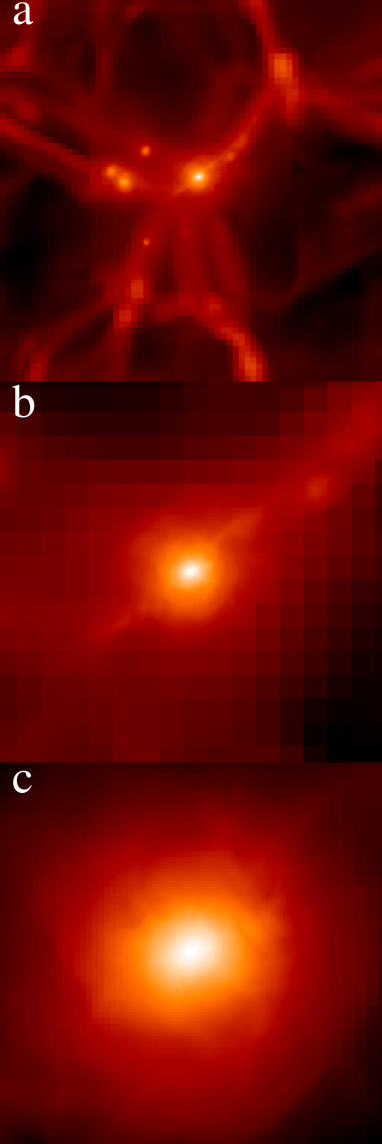
Figure 6: Logarithm of gas column density along z-axis for three centred regions at redshift z=0. From top to bottom: (a) 64 Mpc side image of the gas column density integrate along the central 32 Mpc, (b) 16 Mpc side image of the gas column density integrate along the central 8 Mpc, and (c) 4 Mpc side image of the gas column density integrate along the central 2 Mpc. The ’pixelization’ effect due to the variation in the cell sizes for the different levels is clearly visible.

Figure 6 shows, at the final redshift $z=0$, the gas column density along the z-axis in the different regions. The top panel (a) shows a region of 64 Mpc side length, where the column density has been computed by integrating along the central 32 Mpc. Panels (b) and (c), show the column density maps for two zooms into the central region. The images show regions of 16 and 4 Mpc side, integrated along 8 and 2 Mpc, respectively. The ’pixelization’ effect introduced by the variation in the cell size corresponding to the different levels is clearly visible, as is a web of gaseous filaments linking the structures. It should be noted that there are no unphysical effects associated with filaments crossing the boundaries of patches at different levels.

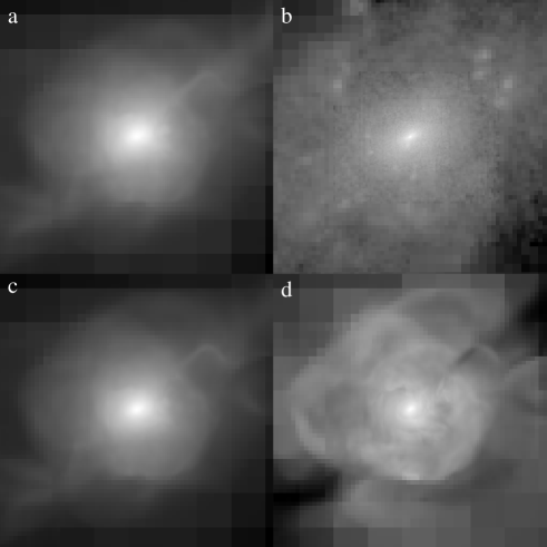
Figure 7: Logarithm of gas column density (a), dark matter column density (b), X-ray surface brightness (c), and emission-weighted temperature(d) along z-axis for the central 8 Mpc at z=0. The image sizes are $8\times 8$ Mpc. As these panels show raw results from the simulations, the ’pixelization’ effect stands out clearly.

In Figure 7, we present several panels displaying maps of the following quantities: a) gas column density, b) dark matter column density , c) X-ray surface brightness calculated as $\int{L_{X}dl}$ where $L_{X}=\rho^{2}T^{1/2}$, and d) emission-weighted temperature calculated as $\int{L_{X}Tdl}/\int{L_{X}dl}$. All images correspond to the projection of these quantities along the z-axis in the 8 Mpc central box. The gross features are similar to the images in F99, although, as the average profiles showed, there are differences in some of the details. The dark matter (Figure 7, panel b) column density looks very similar to results from the highest resolution simulations in F99. Smoothing and presentation effect apart, the substructure in our simulation matches the results from Jenkins & Pearce (SPH) and Bryan & Norman (AMR).

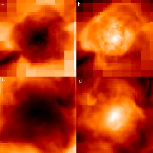
Figure 8: The structure of the shocks and turbulence in the our simulation of the Santa Barbara cluster. Panels (a) and (c) display the entropy in a very thin slice for two zoom-ins at 8 (a) and 2 (c) Mpc. Identically panels (b) and (d) show logarithm of the temperature in the same regions.

The rich structure of shocks, voids, gradients and turbulence can be shown by displaying the entropy and temperature within a thin slice containing the centre of the cluster. Figure 8 displays the entropy and the logarithm of temperature in four thin slices. Upper (lower) panels of Figure 8 show a zoom of the central 8 Mpc (2 Mpc). The images in black and white, are encoded in such a way that black (white) stands for the minimum (maximum) value of the quantity plotted.

The entropy plots show a constant entropy core (panels (a) and (c) in Figure 8). In the temperature maps (panels (b) and (d)) several features are noticeable. A rich structure of shock is visible at all scales. The existence of cold regions embedded in the central hot structure is another remarkable feature. In all cases, a highly turbulent structure is clearly visible. All these features can be studied due to the good shock capturing properties of the algorithm.

The Santa Barbara run has been performed using the parallel version of the code, which has been tested in different architectures. In particular, the run studied in this section was performed in an Origin 3800 using 8 processors, and took 130 hours of CPU time, with a memory requirement of around 2 Gb.

5 Conclusion

We have described and tested a new cosmological code specially designed to study the formation and evolution of cosmological structures, i.e. galaxy cluster, galaxies, etc. The code can follow the hydrodynamics of the gas in a cosmological context, the dark matter component, and the gravity of the two coupled components. The main ingredients of the code are: i) a hydro solver based on high-resolution shock-capturing techniques, ii) a N-body solver based on the generalization of the Particle Mesh scheme, iii) a Poisson solver which combines FFT and SOR techniques, and iv) an Adaptive Mesh Refinement (AMR) scheme which allows us to gain resolution in schemes (i)-(iii) by refining the grid as required according to several application dependent criteria.

A set of tests, including a realistic cosmological simulation known as the Santa Barbara cluster, have been performed so as to explore the reliability of the code. All of them have been passed successfully. The whole package of the different ingredients represents a powerful code which will be able to tackle – with very high spatial and time resolution – all sort of challenging cosmological problems without giving up an accurate description of the physical properties of the gaseous and dark matter components.

Previous results using AMR simulations – with resolution comparable to those of SPH – showed substantial differences in quantities like temperature and entropy with respect to SPH results. This is an important conclusion – confirmed by our simulations – which points out crucial differences between the SPH and the Eulerian methods when describing the physics of structure formation.

AMR codes, like the one presented in this paper, will be essential tools in the future of numerical cosmology. They combine successfully the best properties of previous traditional approaches: i.e. excellent spatial resolution of the SPH techniques, and an accurate description of the hydrodynamics of the problem (handling of shocks and discontinuities, treatment of void regions, accurate thermodynamics, turbulence, and some others) inherited from the Eulerian codes based on Riemann solvers.

In the near future some improvements to the code will be performed. Already as ongoing projects, we are working to incorporate star formation recipes, chemical evolution, cooling, and magnetic fields.

Acknowledgements. VQ is a Ramón y Cajal Fellow of the Spanish Ministry of Science and Technology. This works has been partially supported by grant AYA2003-08739-C02-02 (partially financed with FEDER funds). The author gratefully acknowledges the enlightening comments of the referee and wishes to thank the following for useful discussions and comments: R. Bower, C. Baugh, C.S. Frenk, L. Heck, J.M${}^{\underline{\mbox{a}}}$. Ibáñez, A. Jenkins, J.M${}^{\underline{\mbox{a}}}$. Martí, B. Moore, and T. Okamoto. Simulations were carried out as part of the Virgo Consortium on COSMA at Institute for Computational Cosmology and COSMOS at UK Computational Cosmology Consortium, and in the Servei d’Informática de la Universitat de València (CERCA and CESAR).

References

- [1] Aarseth S.J., 1963, MNRAS, 126, 223
- [2] Anninos P., Norman M.L., Clarke D.A., 1994, ApJ, 436, 11
- [3] Ascasibar Y., Yepes G., Müller V., Gottlöber S., 2003 , 346, 731
- [4] Berger M.J., Colella P., 1989, J. Comp. Phys. 82, 64
- [5] Berger M.J., Oliger J., 1984, J. Comp. Phys., 53, 484
- [6] Bode P., Ostriker J.P., 2003, ApJS, 145, 1
- [7] Bryan G.L., Norman M.L., Stone J.M.m Cen R., Ostriker J.P., 1995, Comput. Phys. Comm., 89, 149
- [8] Bryan G.L., Norman M.L., 1997, in ASP Conf. Ser. 123: Computational Astrophysics; 12th Kingston Meeting on Theoretical Astrophysics, 363
- [9] Blumenthal G.R., Faber S.M., Primack J.R., Rees M.J., 1984, Nature, 311, 517
- [10] Colella P., Woodward P.R., 1984, J. Comp. Phys., 54 174
- [11] Couchman H.M.P., 1991, ApJL, 368, l23
- [12] Davis M., Efstathiou G., Frenk C.S., White S.D.M., 1985, ApJ, 292, 371
- [13] Evrard A.E., 1988, MNRAS, 235, 911
- [14] Frenk C.S. et al., 1999, ApJ, 525, 554
- [15] Gingold R.A., Monaghan J.J., 1977, MNRAS, 181, 375
- [16] Gheller C., Pantano O., Moscardini L., 1998, MNRAS, 295, 519
- [17] Ghigna S, Moore B., Governato F., Lake G., Quinn T., Stadel J., 2000, ApJ, 554, 616
- [18] Gnedin N.Y., 1995, ApJS, 97, 231
- [19] Godunov S.K., 1959, Matematicheskii Sbornik, 47, 271
- [20] Hernquist L., Katz N., 1989, ApJS, 70, 419
- [21] Hockney R.W., Eastwood J.W., 1988, Computer simulation usign particles. IOP Publising
- [22] Jessop C., Duncan M., Chau W.Y., 1994, J. Comp. Phys., 115, 339
- [23] Klypin A., Kravtsov A.V., Bullock J.S., Primack J.R., 2001, ApJ, 554, 903
- [24] Knebe A., Andrew G., Binney J, 2001, MNRAS, 325, 845
- [25] Kravtsov A.V., Klypin A., Hoffman Y., 2002, ApJ, 571, 563
- [26] Kravtsov A.V., Klypin A., Khokhlov A.M., 1997, ApJS, 111, 73
- [27] Laney C.B., 1998, Computational Gasdynamics, Cambridge Univ. Press
- [28] Le Veque R.J., 1992, Numerical methods for conservation laws. Birkhäuser Verlag.
- [29] Lucy L.B., 1977, AJ, 82, 1013
- [30] Okamoto T., Jenkins A., Eke V.R., Quilis V. , Frenk C.S., 2003 , MNRAS, 345, 429
- [31] Peebles P.J.E., 1970, AJ, 75, 13
- [32] Peebles P.J.E., 1980, The large scale structure of the Universe. Princeton University Press.
- [33] Peebles P.J.E., 1982, ApJL, 263, L1
- [34] Pen U.L., 1995, ApJS, 100, 269
- [35] Press W.H., Teukolsky S.A., Vetterling W.T., Flannery B.P., 1996, Numerical Recipes in FORTRAN 77: The Art of Scientific computing. Cambridge University Press
- [36] Power C., Navarro J. F., Jenkins A., Frenk C. S., White S. D. M., Springel V., Stadel J., Quinn T, 2003, MNRAS, 338, 14
- [37] Quilis V., Ibáñez J.M.. Sáez D., 1994, A&A, 286, 1
- [38] Quilis V., Ibáñez J.M.. Sáez D., 1996, ApJ, 469, 11
- [39] Roe P.L., 1981, J. Comp. Phys., 43, 357
- [40] Ruy D., Ostriker J.P., Kang H., Cen R., 1993, ApJ, 414, 1
- [41] Shu C., Osher C., 1988, J. Comp. Phys., 77, 439
- [42] Splinter R.J., 1996, MNRAS, 281, 281
- [43] Springel V., Yoshida N., White S. D. M, 2001, New Astronomy, 6, 79
- [44] Springel V., Hernquist L., 2002, MNRAS, 333, 649
- [45] Teyssier R., 2002, A&A, 385, 337
- [46] Toro E., 1997, Riemann solvers and numerical methods for fluid dynamics, Springer-Verlag
- [47] van Leer B., 1979, J. Comp. Phys., 32, 101
- [48] Villumsen J.V., 1989, ApJS, 71, 407
- [49] White S.D.M., 1976, MNRAS, 177, 717