Electromagnetic Polarization in Partially Ionized Plasmas with Strong Magnetic Fields and Neutron Star Atmosphere Models

Abstract

Polarizability tensor of a strongly magnetized plasma and the polarization vectors and opacities of normal electromagnetic waves are studied for the conditions typical of neutron star atmospheres, taking account of partial ionization effects. Vacuum polarization is also included using a new set of fitting formulae that are accurate for wide range of field strengths. The full account of the coupling of the quantum mechanical structure of the atoms to their center-of-mass motion across the magnetic field is shown to be crucial for the correct evaluation of the polarization properties and opacities of the plasma. The self-consistent treatment of the polarizability and absorption coefficients proves to be necessary if the ionization degree of the plasma is low, which can occur in the atmospheres of cool or ultramagnetized neutron stars. Atmosphere models and spectra are presented to illustrate the importance of such self-consistent treatment.

1. Introduction

In recent years, thermal or thermal-like radiation has been detected from several classes of isolated neutron stars (NSs): radio pulsars with typical magnetic fields $B\sim 10^{12}$–$10^{13}$ G, “dim” NSs whose magnetic fields are mostly unknown, anomalous X-ray pulsars and soft gamma-ray repeaters with $B$ possibly $\sim 10^{14}$–$10^{15}$ G (see, e.g., Becker & Aschenbach, 2002; Haberl, 2004; Israel, Mereghetti, & Stella, 2002; Pavlov & Zavlin, 2003, for reviews). The spectrum of thermal radiation is formed in a thin atmospheric layer (with scale height $\sim 0.1$–$10$ cm and density $\rho\sim 10^{-2}$–$10^{3}$ g cm^-3) that covers the stellar surface. Therefore, a proper interpretation of the observations of NS surface emission requires understanding of radiative properties of these magnetized atmospheres.

Shibanov et al. (1992) (see also Shibanov & Zavlin, 1995; Pavlov et al., 1995) presented the first model of the NS atmospheres with strong magnetic fields, assuming full ionization. Variants of this model were constructed by Zane, Turolla, & Treves (2000, 2001); Ho & Lai (2001, 2003); Özel (2001); Lloyd (2003). An inaccurate treatment of the absorption due to free-free transitions in strong magnetic fields in the earlier models (Pavlov et al., 1995) has been corrected by Potekhin & Chabrier (2003); this correction has been taken into account in later models (Ho et al., 2003, 2004; Lloyd, 2003). Recent work (Ho & Lai, 2003; Lai & Ho, 2002, 2003a) has shown that in the magnetar field regime ($B\gtrsim 10^{14}$ G) vacuum polarization significantly affects the emergent spectrum from the atmosphere; for weaker fields, vacuum polarization can still leave an unique imprint on the X-ray polarization signals (Lai & Ho, 2003b).

Because the strong magnetic field significantly increases the binding energies of atoms, molecules, and other bound states (see Lai, 2001, for a review), these bound states may have abundances appreciable enough to contribute to the opacity in the atmosphere. For calculation of this contribution, the non-trivial coupling of the center-of-mass (CM) motion of the atom to its internal structure (e.g., Potekhin, 1994, and references therein) can be important. Also, because of the relatively high atmosphere density, a proper treatment should take account of the plasma nonideality that leads to Stark broadening and pressure ionization. Recently, thermodynamically consistent equation of state (EOS) and opacities have been obtained for a magnetized, partially ionized H plasma for $8\times 10^{11}$ G $\lesssim B\leq 10^{15}$ G (Potekhin, Chabrier, & Shibanov, 1999; Potekhin & Chabrier, 2003, 2004). These EOS and opacities have been implemented by Ho et al. (2003, 2004) for modeling NS atmospheres. For the typical field strengths $B=10^{12}$–$10^{13}$ G this modeling showed that, although the spectral features due to neutral atoms lie at extreme UV and very soft X-ray energy bands and therefore are difficult to observe, the continuum flux is also different from the fully ionized case, especially at lower energies, which can affect fitting of the observed spectra. For the superstrong field $B\gtrsim 10^{14}$ G, Ho et al. (2003) showed that the vacuum polarization effect not only suppresses the proton cyclotron line, but also suppresses spectral features due to bound species.

It is well known (e.g., Ginzburg, 1970; Mészáros, 1992) that under typical conditions (e.g., far from the resonances) radiation propagates in a magnetized plasma in the form of two so-called extraordinary and ordinary normal modes. The polarization vectors of these modes, $\bm{e}^{\mathrm{X}}$ and $\bm{e}^{\mathrm{O}}$ are determined by the Hermitian part ($\bm{\chi}^{\mathrm{H}}$) of the complex polarizability tensor ($\bm{\chi}$) of the plasma. Our previous treatment of these modes in partially ionized atmospheres (Potekhin & Chabrier, 2003, 2004; Ho et al., 2003, 2004) was not quite self-consistent, because the effect of the presence of the bound states on the polarization of normal modes was neglected: we adopted the same polarization vectors as in the fully ionized plasma, assuming (Potekhin & Chabrier, 2003) that the effect of bound states on these vectors should be small provided the ionization degree of the plasma is high. However, this hypothesis (related to $\bm{\chi}^{\mathrm{H}}$) may be called into question, based on the observation that the absorption coefficients (corresponding to the anti-Hermitian part of the complex polarizability tensor, $i\bm{\chi}^{\mathrm{A}}$) are strikingly affected by the presence of even a few percent of the atoms.

In this paper, we study the polarizability tensor, the polarization vectors of the normal waves, and the opacities of the partially ionized nonideal hydrogen plasma in strong magnetic fields in a self-consistent manner, using the technique applied previously by Bulik & Pavlov (1996) to the case of a monatomic ideal hydrogen gas. In §2 we introduce basic definitions and formulae to be used for calculation of the plasma polarizability (new fitting formulae for the vacuum polarizability are given in the Appendix). An approximate model based on a perturbation theory, which explains the importance of the CM coupling for plasma polarizability, is described in §3. The results of numerical calculations of the plasma polarizability are presented in §4, and the consequences for the polarization and opacities of the normal modes are discussed in §5. In §6 we present examples of NS thermal spectra, calculated using the new opacities, compared with the earlier results. In §7 we summarize our results, outline the range of their applicability, and discuss unsolved problems.

2. General Formulae for Polarization in a Magnetized Plasma

2.1. Complex Polarizability Tensor

The propagation of electromagnetic waves in a medium is described by the wave equation that is obtained from the Maxwell equations involving the tensors of electric permittivity $\bm{\epsilon}$, magnetic permeability $\bm{\mu}$, and electrical conductivity $\bm{\sigma}$. It is convenient (e.g., Ginzburg, 1970) to introduce the complex dielectric tensor $\bm{\epsilon}^{\prime}=\bm{\epsilon}+4\pi i\bm{\sigma}/\omega$. In the strong magnetic field, it should include the vacuum polarization. When the vacuum polarization is small, it can be linearly added to the plasma polarization. Then we can write

$$\bm{\epsilon}^{\prime}=\mathbf{I}+4\pi\bm{\chi}+4\pi\bm{\chi}^{\mathrm{vac}},$$ (1)

where $\mathbf{I}$ is the unit tensor, $\bm{\chi}=\bm{\chi}^{\mathrm{H}}+i\bm{\chi}^{\mathrm{A}}$ is the complex polarizability tensor of the plasma, and $\bm{\chi}^{\mathrm{vac}}$ is the polarizability tensor of the vacuum.

In the Cartesian coordinate system $x^{\prime}y^{\prime}z^{\prime}$ with unit vectors $\hat{\mathbf{x}}^{\prime}$, $\hat{\mathbf{y}}^{\prime}$, $\hat{\mathbf{z}}^{\prime}$, where $\hat{\mathbf{z}}^{\prime}$ is along magnetic field $\bm{B}$, the electric permittivity tensor of a plasma in the dipole approximation, the dielectric vacuum correction, and the inverse magnetic permeability of the vacuum can be written, respectively, as (e.g., Ho & Lai, 2003, and references therein)

$$\mathbf{I}+4\pi{\bm{\chi}}=\left[\begin{array}[]{ccc}\varepsilon&ig&0\\ -ig&\varepsilon&0\\ 0&0&\eta\end{array}\right],$$ (5)

$$4\pi\bm{\chi}^{\mathrm{vac}}=\mathrm{diag}(\hat{a},\hat{a},\hat{a}+q),$$ (6)

$$\bm{\mu}^{-1}=\mathbf{I}+\mathrm{diag}(\hat{a},\hat{a},\hat{a}+m),$$ (7)

where $\hat{a}$, $q$, and $m$ are vacuum polarization coefficients which vanish at $B=0$. The formulae for calculation of these coefficients are given in the Appendix. Quantities $\varepsilon$, $\eta$, and $g$ are well known for fully ionized ideal plasmas (e.g., Ginzburg, 1970). In this paper we shall calculate $\bm{\chi}$ for partially ionized hydrogen plasmas at typical NS atmosphere conditions.

The complex polarizability tensor of a plasma becomes diagonal, $\bm{\chi}=\mathrm{diag}(\chi_{+1},\chi_{-1},\chi_{0})$ in the cyclic or rotating coordinates, where the cyclic unit vectors are defined as $\hat{\mathbf{e}}_{0}=\hat{\mathbf{z}}^{\prime}$, $\hat{\mathbf{e}}_{\pm 1}=(\hat{\mathbf{x}}^{\prime}\pm i\hat{\mathbf{y}}^{\prime})/\sqrt{2}$. The real parts of the components $\chi_{\alpha}$ ($\alpha=\pm 1,0$) determine the Hermitian tensor $\bm{\chi}^{\mathrm{H}}$, which describes the refraction and polarization of waves, and their imaginary parts determine the anti-Hermitian tensor $i\bm{\chi}^{\mathrm{A}}$, responsible for the absorption. According to equation (5),

$$4\pi\chi_{\pm 1}=\varepsilon-1\pm g,\quad 4\pi\chi_{0}=\eta-1.$$ (8)

Note that in the cyclic representation, the general symmetry relations for the polarizability tensor take the form

$$\chi^{\mathrm{A}}_{\alpha}(-\omega)=-\chi^{\mathrm{A}}_{-\alpha}(\omega),\quad\chi^{\mathrm{H}}_{\alpha}(-\omega)=\chi^{\mathrm{H}}_{-\alpha}(\omega).$$ (9)

2.2. Relation Between the Plasma Polarizability and Absorption

General expressions in the dipole approximation for $\chi^{\mathrm{A}}_{\alpha}$ and $\chi^{\mathrm{H}}_{\alpha}$ through frequencies and oscillator strengths of quantum transitions in a magnetized medium are given, e.g., by Bulik & Pavlov (1996). For transitions between two stationary quantum states $i$ and $f$ with energies $E_{i}$ and $E_{f}=E_{i}+\hbar\omega_{fi}>E_{i}$ and number densities of the occupied states $n_{i}$ and $n_{f}$, the absorption coefficient for the basic polarization $\alpha$ equals (see, e.g., Armstrong & Nicholls, 1972)

$$\mu^{if}_{\alpha}\equiv\rho\hat{\kappa}_{\alpha}(\omega)=\frac{2\pi^{2}e^{2}}{m_{e}c}\,(n_{i}-n_{f})\,f^{if}_{\alpha}\delta(\omega-\omega_{fi}),$$ (10)

where $f^{if}_{\alpha}=(2m_{e}\omega_{fi}/\hbar)\,|\langle f|\bm{r}|i\rangle\cdot\hat{\mathbf{e}}_{\alpha}|^{2}$ is the oscillator strength for the transition $i\rightarrow f$. These partial absorption coefficients sum up into the total $\mu_{\alpha}=\sum_{i,f(E_{f}>E_{i})}\mu^{if}_{\alpha}$, where $\sum_{i,f}$ includes integration over continuum states. Then the equation

$$\chi^{\mathrm{A}}_{\alpha}(\omega)=\frac{c}{4\pi\omega}\,\mu_{\alpha}(\omega),$$ (11)

together with the first symmetry relation (9) yield

$$\chi^{\mathrm{A}}_{\alpha}(\omega) = \frac{\pi e^{2}}{2m_{e}\omega}\,\sum_{i,f(E_{f}>E_{i})}(n_{i}-n_{f})$$ (12)

$$\times\left[f^{if}_{\alpha}\,\delta(\omega-\omega_{fi})+f^{if}_{-\alpha}\,\delta(\omega+\omega_{fi})\right].$$

Once $\chi^{\mathrm{A}}$ is known, $\chi^{\mathrm{H}}$ can be calculated from the Kramers-Kronig relation (Landau & Lifshitz, 1989, §123) or its modification (Bulik & Pavlov, 1996),

$$\chi^{\mathrm{H}}_{\alpha}(\omega)=\frac{1}{\pi\omega}\,\mathcal{P}\int_{-\infty}^{\infty}\frac{\omega^{\prime}\chi^{\mathrm{A}}_{\alpha}(\omega^{\prime})}{\omega^{\prime}-\omega}\,\mathrm{d}\omega^{\prime},$$ (13)

where $\mathcal{P}\!\int$ means the principal value of the integral. From equations (12) and (13),

$$\chi^{\mathrm{H}}_{\alpha}(\omega)=-\frac{e^{2}}{2\,m_{e}\omega}\!\!\!\!\!\!\sum_{i,f\,(E_{f}>E_{i})\rule{0.0pt}{6.02777pt}}\!\!\!\!\!\!(n_{i}-n_{f})\left[\frac{f^{if}_{\alpha}}{\omega-\omega_{fi}}+\frac{f^{if}_{-\alpha}}{\omega+\omega_{fi}}\right].$$ (14)

Taking into account equations (11) and (9), we can present relation (13) in the form convenient for calculation at $\omega>0$:

$$\chi^{\mathrm{H}}_{\alpha}(\omega) = \frac{c}{4\pi^{2}\omega}\,\bigg{\{}\int_{0}^{\omega}\big{[}\,\mu_{\alpha}(\omega+\omega^{\prime})-\mu_{\alpha}(\omega-\omega^{\prime})\,\big{]}\frac{\mathrm{d}\omega^{\prime}}{\omega^{\prime}}$$ (15)

$$+\int_{2\omega}^{\infty}\frac{\mu_{\alpha}(\omega^{\prime})}{\omega^{\prime}-\omega}\,\mathrm{d}\omega^{\prime}-\int_{0}^{\infty}\frac{\mu_{-\alpha}(\omega^{\prime})}{\omega^{\prime}+\omega}\,\mathrm{d}\omega^{\prime}\bigg{\}}.$$

If we replace delta-function in equation (10) by the Lorentz profile $(\nu^{if}_{\alpha}/\pi)\,[\,(\omega-\omega_{\alpha})^{2}+(\nu^{if}_{\alpha})^{2}\,]^{-1}$, where $\nu^{if}_{\alpha}$ is a damping rate for a given transition, then equations (12) and (14) can be combined to give

$$\chi_{\alpha}(\omega) = -\frac{e^{2}}{2\,m_{e}\omega}\sum_{i,f\,(E_{f}>E_{i})}(n_{i}-n_{f})\Bigg{[}\frac{f^{if}_{\alpha}}{\omega-\omega_{fi}+i\nu^{if}_{\alpha}}$$ (16)

$$+\frac{f^{if}_{-\alpha}}{\omega+\omega_{fi}+i\nu^{if}_{-\alpha}}\Bigg{]}.$$

3. Analytic Model of Polarization of Atomic Gas: Effect of Center-of-Mass Motion

As mentioned in §1, in strong magnetic fields the internal structure of an atom is strongly coupled to its CM motion perpendicular to the field. This coupling (referred to as “CM coupling”) has a significant effect on the radiative opacities and dielectric property of the medium. Before presenting numerical results for the polarizability tensor of a partially ionized plasma in §4, it is useful to consider an analytic model to illustrate this CM coupling effect.

Consider an atomic gas in which the atom possesses only two energy levels, with the upper level having the radiative (Lorentz) width $\nu$, assumed to be constant for simplicity. The energies of the (moving) atom in the ground state and the excited state are denoted by $E_{1}(\bm{P})$ and $E_{2}(\bm{P}^{\prime})$ respectively, where $\bm{P}$ and $\bm{P}^{\prime}$ are the CM pseudo-momenta, and the subscripts 1 and 2 specify the internal degree of freedom of the atom. [In strong magnetic fields, the internal quantum numbers are $(s,\nu_{z})$, where $s=0,1,2,\cdots$ measures the relative angular momentum between the proton and electron, and $\nu_{z}$ is related to the number of nodes in the $z$ direction.] If there were no CM coupling, we would have $E_{1,2}(\bm{P})=E_{1,2}(0)+\bm{P}^{2}/(2m_{\mathrm{H}})$ and $\omega_{21}\equiv(E_{2}-E_{1})/\hbar=$constant. Therefore, in this case equation (16) would yield

$$\chi_{\alpha}(\omega)\simeq-\,{e^{2}n_{1}\over 2m_{e}\omega}\left[{f_{\alpha}^{12}\over\omega-\omega_{21}+i\nu}+{f_{-\alpha}^{12}\over\omega+\omega_{21}+i\nu}\right].$$ (17)

This would imply that even for very small neutral atom fraction, the bound-bound transition can severely affect the dielectric property of the gas in the neighborhood of $\omega=\omega_{21}$ (for $\nu\ll\omega_{21}$).

However, in strong magnetic fields, the energy associated with the transverse CM motion of the atom cannot be separated from the internal energy. We therefore have

$$\chi_{\alpha}(\omega) = -{e^{2}n_{1}\over 2m_{e}\omega}\int\!{p_{1}(P_{\perp})\,\mathrm{d}^{2}P_{\perp}\over(2\pi\hbar)^{2}}\bigg{[}\frac{f_{\alpha}^{12}(\bm{P}_{\perp})}{\omega-\omega_{21}(P_{\perp})+i\nu}$$ (18)

$$+\frac{f_{-\alpha}^{12}(\bm{P}_{\perp})}{\omega+\omega_{21}(P_{\perp})+i\nu}\bigg{]},$$

where $\bm{P}_{\perp}$ is the transverse pseudo-momentum, $p_{1}(P_{\perp})\,\mathrm{d}^{2}P_{\perp}$ is the probability to find an atom in the initial state “1” in an element $\mathrm{d}^{2}P_{\perp}$ near $\bm{P}_{\perp}$ (see Potekhin et al., 1999), and we have used the fact that the oscillator strength is nonzero only when $\bm{P}=\bm{P}^{\prime}$ (in the dipole approximation). The CM coupling effect will significantly smooth out the divergent behavior at $\omega=\omega_{21}$ in equation (17) (for $\nu\rightarrow 0$). This effect can be taken into account using the perturbation result of Pavlov & Mészáros (1993), as was done by Bulik & Pavlov (1996), or numerically, using the techniques of Pavlov & Potekhin (1995) and Potekhin & Pavlov (1997).

In the perturbation theory, valid for small $P_{\perp}$, the coupling reveals itself as an effective “transverse” mass $M_{\perp}>m_{\mathrm{H}}$ acquired by the atom, which is different for different quantum levels. For the two-level atom, the perturbation theory gives $E_{j}(P_{\perp})=E_{j}(0)+P_{\perp}^{2}/(2M_{\perp j})$ ($j=1,2$), and we find

$$\chi_{\alpha} \simeq -\frac{e^{2}n_{1}}{2m_{e}\omega}\int_{0}^{\infty}\!\mathrm{d}y\bigg{[}\frac{f_{\alpha}^{12}\,e^{-y}}{\omega-\omega_{21}(0)+i\nu+a(T)\,y}$$ (19)

$$+\frac{f_{-\alpha}^{12}\,e^{-y}}{\omega+\omega_{21}(0)+i\nu+a(T)\,y}\bigg{]},$$

where $a(T)=(k_{\mathrm{B}}T/\hbar)(1-M_{\perp 1}/M_{\perp 2})$, and we have used $p_{1}(P_{\perp})\propto\exp[-P_{\perp}^{2}/(2M_{\perp 1}k_{\mathrm{B}}T)]$. At $\nu\to 0$, only weak logarithmic divergence is present near $\omega=\omega_{21}$, compared to the much stronger $(\omega-\omega_{21})^{-1}$ divergence in equation (17). Additional line broadening due to collisions (which implies $\nu\neq 0$), thermal effect and pressure effect, not treated in this simple model, will further smooth out the “divergent” feature in the polarizability tensor.

This simple model shows that a proper treatment of the CM coupling is important in calculating the polarizability tensor of a partially ionized plasma. In practice, since the absorption coefficient $\mu_{\alpha}$ has already been calculated by Potekhin & Chabrier (2003, 2004), we find it is more convenient to apply the Kramers-Kronig transformation (eq. [15]) to obtain $\chi^{\mathrm{H}}_{\alpha}$ (see §4).

4. Effect of Partial Ionization on Polarizability of a Strongly Magnetized Hydrogen Plasma

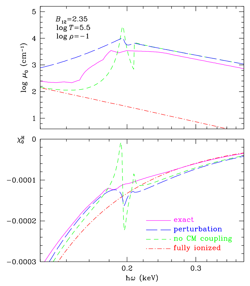
Figure 1.— Absorption coefficient (upper panel) and polarizability (lower panel) of a hydrogen plasma for longitudinal polarization ($\alpha=0$) at $B=2.35\times 10^{12}$ G, $\rho=0.1$ g cm^-3, and $T=3.16\times 10^{5}$ K, according to four different models: fully ionized plasma (dot-dashed lines), partially ionized plasma without the effect of coupling between CM motion and internal structure of the atom (short dashes), with the magnetic broadening taken into account by perturbation theory (long dashes) and numerical calculation beyond the perturbation approximation (solid lines).

Some approximations for calculation of the complex dielectric tensor of a plasma have been discussed, for example, by Ginzburg (1970). In particular, the “elementary theory” gives the expression widely used in the past to describe polarization properties of the fully ionized electron-ion plasma (e.g., Shibanov et al., 1992; Zane et al., 2000; Ho & Lai, 2001, 2003):

$$4\pi\chi_{\alpha}=-\frac{\omega_{\mathrm{pl}}^{2}}{(\omega+\alpha\omega_{\mathrm{c}e})(\omega-\alpha\omega_{\mathrm{ci}})+i\omega\nu_{\mathrm{eff}}},$$ (20)

where $\omega_{\mathrm{c}e}=eB/m_{e}c$ and $\omega_{\mathrm{ci}}=ZeB/m_{\mathrm{i}}c$ are the electron and ion cyclotron frequencies, $\omega_{\mathrm{pl}}=(4\pi n_{e}e^{2}/m_{e})^{1/2}$ is the electron plasma frequency, $\nu_{\mathrm{eff}}$ is the effective damping frequency, $m_{\mathrm{i}}$ is the ion mass, $Ze$ is the ion charge, and $n_{e}$ is the electron number density. For the hydrogen plasma, the corresponding energies are $\hbar\omega_{\mathrm{c}e}=11.577\,B_{12}$ keV, $\hbar\omega_{\mathrm{ci}}=6.3049\,B_{12}$ eV, where $B_{12}=B/10^{12}$ G, and $\hbar\omega_{\mathrm{pl}}=0.0287\sqrt{\rho}$ keV, where $\rho$ is in g cm^-3. In general, the damping frequency $\nu_{\mathrm{eff}}$ depends on polarization and photon frequency. Derivation of equation (20) is based on the assumption that the electrons and ions lose their ordered velocities (imparted by the electric field of the electromagnetic wave) at the rate $\nu_{\mathrm{eff}}$ which does not depend on the velocity. A more rigorous kinetic theory gives $\chi^{\mathrm{A}}_{\alpha}$ and $\chi^{\mathrm{H}}_{\alpha}$ which cannot be in general described by equation (20) using the same $\nu_{\mathrm{eff}}$ (e.g., Ginzburg, 1970, §6). For instance, if we describe $\chi^{\mathrm{A}}_{\alpha}$ using equation (20) with some frequency-dependent $\nu_{\mathrm{eff}}(\omega)$, then the Kramers-Kronig transformation will give $\chi^{\mathrm{H}}_{\alpha}$ which, in general, does not coincide with the real part of equation (20) with the same $\nu_{\mathrm{eff}}(\omega)$, although, for realistic $\nu_{\mathrm{eff}}(\omega)$, the difference should be small at $\omega\gg\omega_{\mathrm{pl}}$.

Realistic models of the absorption coefficients of a partially ionized plasma do not allow us to perform the Kramers-Kronig transformation analytically. We evaluated the integrals in equation (15) numerically. Since the integrand can be sharply peaked near resonance frequencies, we employed the adaptive-stepsize Runge-Kutta integration (Press et al., 1996, §16.2). The accuracy of the numerical transformation was tested with the models that allow one to perform the Kramers-Kronig transformation analytically – those given by equations (17) and (20) above, and by equations (49)–(53) of Bulik & Pavlov (1996) – and proved to be within 0.1%.

Let us first consider a model that neglects the CM coupling and the plasma nonideality. The absorption coefficient of the fully ionized component of the plasma includes contributions due to the free-free absorption and scattering on free electrons an protons. For the atoms, we include in consideration the bound-bound transition with the largest oscillator strength (for every polarization) and the bound-free transitions. In this case the absorption by the atom can be described by analytic formulae. The bound-bound absorption cross section is described by the Lorentz profile, where the effective damping width is mainly contributed by the electron impact broadening (Pavlov & Potekhin, 1995) and can be evaluated using a fitting formula (Potekhin, 1998). The bound-free cross sections are well described in the adiabatic approximation (however this is not true with the CM coupling, see Potekhin & Pavlov 1997); they are reproduced by fitting formulae in Potekhin & Pavlov (1993). For $B=2.35\times 10^{12}$ G, $\rho=0.1$ g cm^-3, $T=10^{5.5}$ K (the neutral fraction $x_{\mathrm{H}}\approx 0.12$), the resulting absorption coefficients are shown by the short-dashed lines in Figures 1 and 2 for $\alpha=0$ and $+1$, respectively. For $\alpha=0$ this absorption profile is similar to the idealized model considered above. The corresponding $\chi^{\mathrm{H}}_{\alpha}(\omega)$ are shown by the short-dashed lines on the lower panels of Figures 1 and 2. In each figure, dot-dashed lines correspond to the model of a fully ionized hydrogen plasma at the same $B$, $\rho$, and $T$. As in the above analytic model, we see that the presence of the atoms results in strong deviation from the fully ionized plasma model in the vicinity of the principal atomic resonances (the bound-free resonance for $\alpha=+1$ is almost invisible on the lower panel of Fig. 2 because of its small oscillator strength).

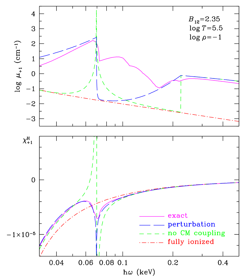
Figure 2.— Same as in Figure 1, but for $\alpha=+1$.

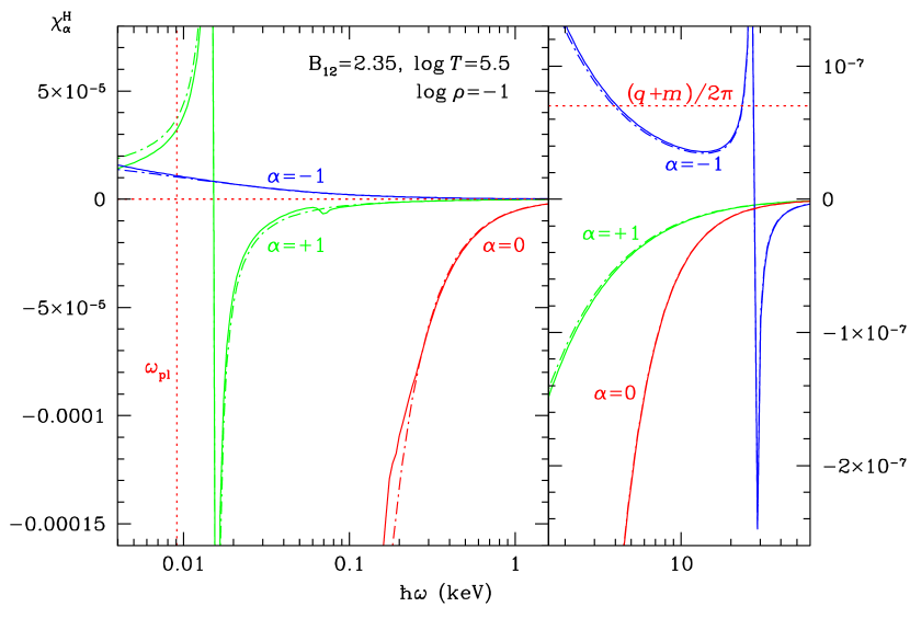
Figure 3.— Polarizabilities $\chi^{\mathrm{H}}_{\alpha}$ ($\alpha=\pm 1,0$) of the partially ionized (solid lines) and fully ionized (dot-dashed lines) plasma with the same parameters as in Figures 1, 2. The right part of the figure has an enlarged vertical scale. The dotted lines correspond to $\omega_{\mathrm{pl}}$ (vertical) and $(q+m)/(2\pi)$ (horizontal), where $q$ and $m$ are the vacuum polarization parameters.

The absorption coefficients obtained using the perturbation theory of magnetic broadening (§3) are shown by the long-dashed lines on the upper panels of Figures 1 and 2. The long-dashed lines on the lower panels show the corresponding polarizabilities. We see that the resonant features are smoothed down by the magnetic broadening, and the resulting curves of $\chi^{\mathrm{H}}_{\alpha}(\omega)$ do not much differ from the fully ionized plasma model.

Still greater smoothing occurs for the accurate (nonperturbative) functions $\mu_{\alpha}(\omega)$ and $\chi^{\mathrm{H}}_{\alpha}(\omega)$ (solid lines in the figures). The absorption coefficients shown on the upper panels correspond to the opacities in Figure 9 of Potekhin & Chabrier (2003). The significant difference of these absorption coefficients from the perturbational ones arises partly from the dependence of the oscillator strengths on the atomic velocity across the field, partly from transitions which were dipole-forbidden for the atom at rest and were not taken into account in the perturbation approximation described above, and partly from the nonideal plasma effect of continuum lowering. Nevertheless, despite these differences in $\mu_{\alpha}$, the difference in $\chi^{\mathrm{H}}_{\alpha}$ is much less significant.

Figure 3 shows all three components $\chi^{\mathrm{H}}_{\alpha}$ in a wider energy range. In this figure, as well as in the previous two, the polarizabilities in the fully ionized plasma model, shown by the dot-dashed lines, are obtained from equation (15), where the free-free contribution to $\mu_{\alpha}(\omega)$ includes the frequency-dependent Coulomb logarithm $\Lambda_{\alpha}^{\mathrm{ff}}$ (Potekhin & Chabrier, 2003). Because of this frequency dependence, these polarizabilities are not identical to the ones given by equation (20), the difference being small at $\omega\gg\omega_{\mathrm{pl}}$ and appreciable at $\omega\lesssim\omega_{\mathrm{pl}}$, where both the elementary theory and the description of absorption by binary collisions (i.e., neglecting the collective motion effects) are rather inaccurate. The solid lines, which are obtained for the partially ionized plasma, are fairly close to the dot-dashed lines. The only prominent features are the proton and electron cyclotron resonances at $\hbar\omega_{\mathrm{ci}}=0.0148$ keV and $\hbar\omega_{\mathrm{c}e}=27.21$ keV.

However, such smoothing does not always occur. Let us consider a higher magnetic field $B=3\times 10^{13}$ G and density $\rho=1$ g cm^-3, retaining the same temperature. Then $x_{\mathrm{H}}=0.89$. Figure 4 demonstrates the absorption coefficients and polarizabilities for the fully ionized (dot-dashed lines) and partially ionized (solid lines) plasma. In addition to the proton cyclotron resonance at $\hbar\omega=0.19$ keV, absorption coefficients in the partially ionized plasma exhibit magnetically broadened bound-bound and bound-free features. The most prominent are the bound-bound absorption at $\hbar\omega\approx 0.2$–0.3 keV for $\mu_{+1}$ and the photoionization edge at $\hbar\omega=0.408$ keV for $\mu_{0}$. These features are clearly reflected in the behavior of $\chi^{\mathrm{H}}_{+1}$ and $\chi^{\mathrm{H}}_{0}$, shown in the lower panels. Thus, with increasing $B$, the abundance of neutral states increases along with their influence on the polarizability.

A similar trend occurs with lowering $T$. If, for example, in the previous case ($B=2.35\times 10^{12}$ G, $\rho=0.1$ g cm^-3) we take a lower $T=1.58\times 10^{5}$ K, then we will have 94.1% of H atoms in the ground state, 1.3% in the excited states, and 1.1% of H₂ molecules. At $\rho=1$ g cm^-3, the abundance of the atoms will be 96.9% (with roughly equal fractions of excited states and molecules), and we nearly recover the case studied by Bulik & Pavlov (1996), who assumed 100% of atoms for these plasma parameters.

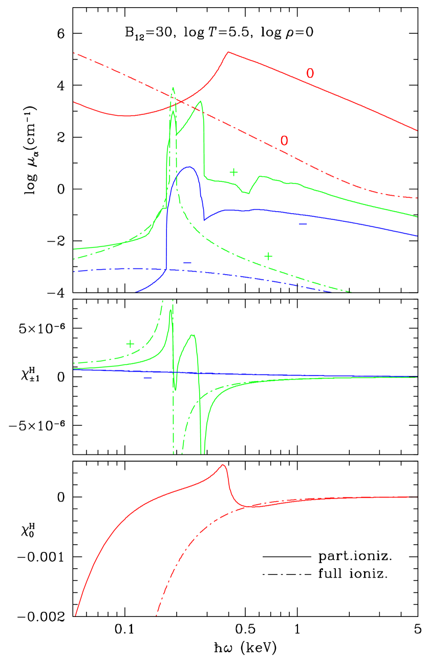
Figure 4.— Absorption coefficients (top panel; the lines marked “+”, “$-$”, and “0” correspond to the polarization index $\alpha=+1$, $-1$, and $0$, respectively) and polarizabilities $\chi^{\mathrm{H}}_{\pm 1}$ (middle) and $\chi^{\mathrm{H}}_{0}$ (bottom panel) of the partially ionized (solid lines) and fully ionized (dot-dashed lines) plasma for $B=3\times 10^{13}$ G, $\rho=1$ g cm^-3, and $T=3.16\times 10^{5}$ K.

5. Effect of Partial Ionization on Polarization and Opacities of Normal Modes

In the coordinate system $xyz$ with $z$ along the wave vector of the photon and $\bm{B}$ in the $x$–$z$ plane, the polarization vectors $\bm{e}^{j}$ of the normal modes in a magnetized plasma can be written as (Ho & Lai, 2003)

$$(e^{j}_{x},e^{j}_{y},e^{j}_{z})=(1+K_{j}^{2}+K_{z,j}^{2})^{-1/2}\,(iK_{j},1,iK_{z,j}),$$ (21)

where $j=1,2$ correspond to the extraordinary mode (X-mode) and ordinary mode (O-mode). The parameters $K_{j}$ and $K_{z,j}$ are expressed in terms of the components of the dielectric and magnetic tensors as

$$K_{j}=\beta\left\{1+(-1)^{j}\left[1+\frac{1}{\beta^{2}}+\frac{m}{1+\hat{a}}\frac{\sin^{2}\theta_{B}}{\beta^{2}}\right]^{1/2}\right\},$$ (22)

$$K_{z,j}=-\frac{(\varepsilon^{\prime}-\eta^{\prime})K_{j}\cos\theta_{B}+g}{\varepsilon^{\prime}\sin^{2}\theta_{B}+\eta^{\prime}\cos^{2}\theta_{B}}\,\sin\theta_{B},$$ (23)

where

$$\beta=\frac{\eta^{\prime}-\varepsilon^{\prime}+g^{2}/\varepsilon^{\prime}+\eta^{\prime}\,m/(1+\hat{a})}{2\,g}\,\frac{\varepsilon^{\prime}}{\eta^{\prime}}\,\frac{\sin^{2}\theta_{B}}{\cos\theta_{B}},$$ (24)

$\theta_{B}$ is the angle between $\bm{B}$ and the $z$ axis, and (see Eqs. [1]–[6]) $\varepsilon^{\prime}=\varepsilon+\hat{a}$, $\eta^{\prime}=\eta+\hat{a}+q$. In the usual case where the plasma and vacuum polarizabilities are small ($|\chi^{\mathrm{H}}_{\alpha}|\ll(4\pi)^{-1}$ and $|\hat{a}|,q,|m|\ll 1$), the polarization parameter $\beta$ is given by

$$\beta\approx\frac{2\chi^{\mathrm{H}}_{0}-\chi^{\mathrm{H}}_{+1}-\chi^{\mathrm{H}}_{-1}+(q+m)/(2\pi)}{2\,(\chi^{\mathrm{H}}_{+1}-\chi^{\mathrm{H}}_{-1})}\,\frac{\sin^{2}\theta_{B}}{\cos\theta_{B}}.$$ (25)

The opacity in the mode $j$ can be written as

$$\kappa_{j}(\omega,\theta_{B})=\sum_{\alpha=-1}^{1}\!\!|e_{\alpha}^{j}(\omega,\theta_{B})|^{2}\,\hat{\kappa}_{\alpha}(\omega),$$ (26)

where $\hat{\kappa}_{\alpha}$ ($\alpha=-1,0,1$) do not depend on $\theta_{B}$. For a partially ionized, strongly magnetized hydrogen plasma $\hat{\kappa}_{\alpha}(\omega)$ have been obtained by Potekhin & Chabrier (2003, 2004).

The polarization vectors $\bm{e}^{\mathrm{X}}$ and $\bm{e}^{\mathrm{O}}$ for the polarizabilities presented in Figure 3 prove to be indistinguishable from the results for the fully ionized plasma at general $\theta_{B}$ values. They exhibit vacuum polarization resonances at $\hbar\omega\sim 10$ keV related to intersections of $\chi^{\mathrm{H}}_{-1}$ with the combination of vacuum polarization coefficients $(q+m)/2\pi$ that enters equation (25) (the horizontal dotted line in Fig. 3; in this case $|\chi^{\mathrm{H}}_{0}|,|\chi^{\mathrm{H}}_{+1}|\ll|\chi^{\mathrm{H}}_{-1}|$) and the electron cyclotron resonance at $\hbar\omega\approx 27$ keV. If we neglected the CM coupling effect, we would observe additional resonant features near $\hbar\omega=0.07$ and 0.2 keV, associated with the bound-bound transitions for $\alpha=+1$ (Fig. 2) and $\alpha=0$ (Fig. 1). Actually these features are smoothed away by the CM coupling.

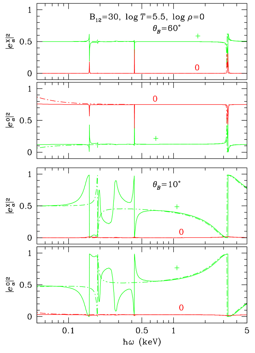
Figure 5.— Squared moduli of the cyclic components $e^{j}_{\alpha}$ of polarization vectors $\bm{e}^{\mathrm{X}}$ and $\bm{e}^{\mathrm{O}}$ for the normal waves propagating at angles $\theta_{B}=60^{\circ}$ (two upper panels) and $10^{\circ}$ (two lower panels) in a hydrogen plasma with $B=3\times 10^{13}$ G, $T=3.16\times 10^{5}$ K, $\rho=1$ g cm^-3. Solid lines: partially ionized plasma; dot-dashed lines: full ionization.

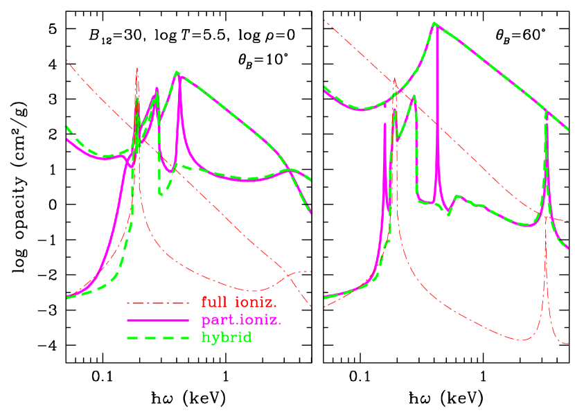
Figure 6.— Opacities in two modes $\kappa_{j}$ (Eq. [26]) for the same plasma parameters as in Fig. 5 and two angles, $\theta_{B}=10^{\circ}$ (left panel) and $\theta_{B}=60^{\circ}$ (right panel). Solid lines: a self-consistent calculation for a partially ionized hydrogen plasma; dashed lines: partially ionized hydrogen plasma within a “hybrid” treatment (a model that uses the basic opacities $\hat{\kappa}_{\alpha}$ from the model of partially ionized plasma and polarization vectors $\bm{e}^{j}$ from the model of full ionization); light dot-dashed lines: model of full ionization. The lower curve of each type is related to extraordinary and the upper one to ordinary mode (the dashed curve often coincides with the solid one).

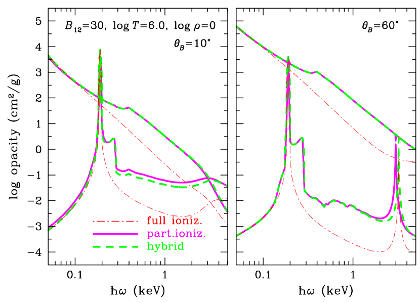
Figure 7.— Same as in Fig. 6 but for higher temperature, $T=10^{6}$ K.

For the second set of plasma parameters considered in §4, the ionization degree is relatively low ($1-x_{\mathrm{H}}=0.11$). Figure 5 shows squared moduli of two components of the polarization vectors, $e^{j}_{0}$ and $e^{j}_{+1}$ (the third component can be found as $|e_{-1}|^{2}=1-|e_{+1}|^{2}-|e_{0}|^{2}$) for two propagation angles $\theta_{B}=60^{\circ}$ and $\theta_{B}=10^{\circ}$. Dot-dashed and solid curves correspond to the fully and partially ionized plasma models, respectively. At $\theta_{B}=60^{\circ}$ (two upper panels), there are two sharp resonances for the partially ionized case at $\hbar\omega=0.158$ and 0.425 keV, associated with the zero level crossings by $\chi^{\mathrm{H}}_{0}(\omega)$ (the bottom panel of Fig. 4), which are absent in the case of full ionization. The feature at 3.3 keV is the vacuum resonance. At smaller angle (two lower panels of Fig. 5), these resonances become broader, and there appear additionally other features associated with the behavior of $\chi^{\mathrm{H}}_{+1}$ (see the middle panel of Fig. 4). For the fully ionized plasma, an additional feature is just the proton cyclotron resonance, whereas for the partially ionized case the behavior of the polarization vectors is more complicated because of the influence of the atomic resonances.

Figure 6 shows the opacities calculated according to equation (26), using $|e^{j}_{\alpha}|^{2}$ shown in Figure 5 and $\hat{\kappa}_{\alpha}(\omega)$ calculated as in Potekhin & Chabrier (2003, 2004). The opacities that take into account partial ionization are plotted by solid lines, and those assuming full ionization by dot-dashed lines. The dashed lines correspond to a hybrid approach, where the polarization of normal modes is described by the formulae for a fully ionized plasma, and $\hat{\kappa}_{\alpha}(\omega)$ take into account bound-bound and bound-free atomic transitions (Potekhin & Chabrier, 2003). Although this approach is closer to reality than the model of full ionization, there are significant differences from the more accurate result drawn by the solid lines. In particular, the feature near $\hbar\omega=0.5$ keV is missed in the hybrid approximation.

With increasing temperature, the differences between the self-consistent and hybrid approximations go away. Figure 7 shows the case where the plasma parameters are the same as in Figure 6, except for $T=10^{6}$ K. At this temperature, $x_{\mathrm{H}}=1.4$%. Such small amount of neutral atoms is still very important for the opacities, but the hybrid approximation yields the result close to self-consistent one.

Summarizing, we conclude that the hybrid approach to calculation of the mode opacities can be applicable if the fraction of bound states in the plasma, $x_{\mathrm{H}}$ is small.

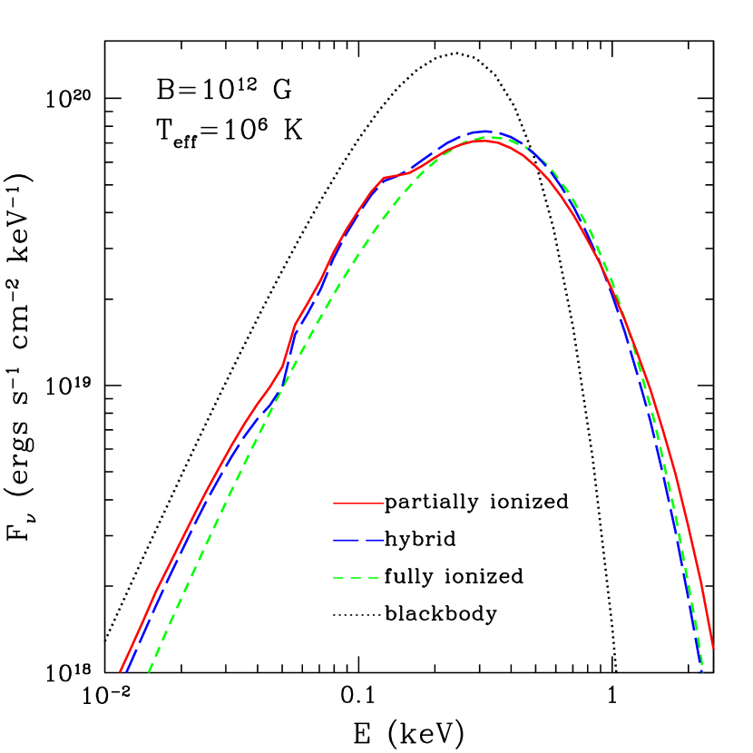
Figure 8.— Spectrum of hydrogen atmosphere with $B=10^{12}$ G (field normal to the surface) and effective temperature $T_{\mathrm{eff}}=10^{6}$ K. The solid line is for the self-consistent model of a partially ionized atmosphere, the long-dashed line is for the hybrid model, the short-dashed line is for a fully ionized atmosphere, and the dotted line is for a blackbody with $T=T_{\mathrm{eff}}$.

6. Spectra

Examples of application of the self-consistent opacity calculation for partially ionized hydrogen NS atmospheres are given in Figures 8–10. Here, the atmosphere parameters are the same as for the low-field models in Ho et al. (2003). The solid lines are obtained using the self-consistent calculation of the opacities, while the long-dashed lines reproduce the hybrid treatment described above. The fully ionized plasma model (short dashes) and blackbody (dots) are shown for comparison. The difference in the spectra obtained using the self-consistent and hybrid approaches is partly due to the difference in the temperature profiles within the atmosphere. As expected, this difference is small at relatively low magnetic field $B=10^{12}$ G and effective temperature $T_{\mathrm{eff}}=10^{6}$ K (Fig. 8), where the fraction of atoms is small at every optical depth in the atmosphere, but it becomes larger for lower temperature ($T_{\mathrm{eff}}=5\times 10^{5}$ K, Fig. 9) or stronger field ($B=10^{13}$ G, Fig. 10). In the case shown in Figure 9, the temperature profile $T(\rho)$ calculated with the new (self-consistent) opacities is higher by $\sim 10$%, so that photons come from shallower (lower atomic fraction) layers of the atmosphere, which results in weaker spectral features due to the atomic transitions. A modification of the temperature profile is also responsible for the weaker proton cyclotron feature in this case. At contrast, in the case shown in Figure 10 the temperature profile is lower by $\lesssim 10$%, and photons come from deeper (higher atomic fraction) layers, resulting in stronger atomic features.

For superstrong fields ($B\gtrsim 10^{14}$ G), the current atmosphere models are less reliable because of the unsolved problems of mode conversion and dense plasma effect (e.g., Ho et al., 2003), whose importance increases with increasing $B$.

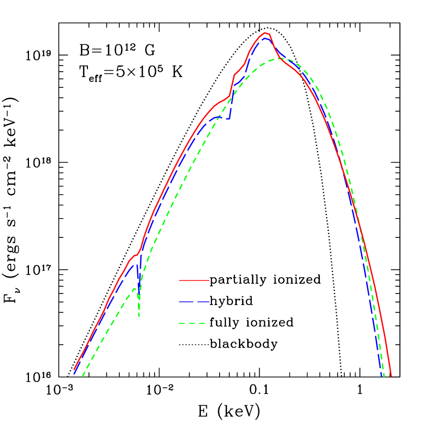
Figure 9.— Same as in Fig. 8 but for lower effective temperature, $T_{\mathrm{eff}}=5\times 10^{5}$ K.

7. Conclusions and Outlook

We have studied the polarizability and electromagnetic polarization modes in a partially ionized, strongly magnetized hydrogen plasma. The full account of the coupling of the quantum mechanical structure of the atoms to their center-of-mass motion across the magnetic field is shown to be crucial for the correct evaluation of the polarization properties and opacities of the plasma. The self-consistent treatment of the polarizability and absorption coefficients is ensured by use of the Kramers-Kronig relation. Such treatment proves to be important if the ionization fraction of the plasma is low ($\lesssim 50$%). For high degree of ionization ($\gtrsim 80$%), the polarizability of a fully ionized plasma remains a good approximation, just as previously assumed (Potekhin & Chabrier, 2003). This approximation was adopted in the NS atmosphere models built in Ho et al. (2003, 2004). A comparison with updated spectra based on the self-consistent treatment (§6) shows that this approximation is satisfactory if $B\lesssim 10^{13}$ G and $T_{\mathrm{eff}}\gtrsim 10^{6}$ K. The self-consistent treatment is needed in the atmospheres of cool or ultramagnetized NSs, with relatively low degrees of ionization.

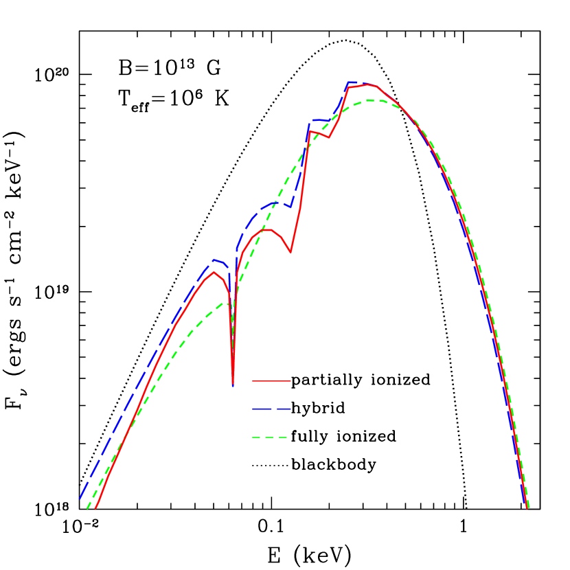
Figure 10.— Same as in Fig. 8 but for higher field strength, $B=10^{13}$ G.

There are several limitations of the present model, which may become important for the magnetar fields and/or for low $T_{\mathrm{eff}}$. While H atoms are treated accurately in our calculations of the EOS and opacities, H₂ molecules are included in the EOS using the static approximation (i.e., without their CM coupling) and neglected in the opacities. Other bound species, such as H₂⁺ (e.g., Turbiner & López Vieyra, 2003), H₃²⁺ (López Vieyra & Turbiner, 2000), and H_n chains (Lai, Salpeter, & Shapiro, 1992) are not included. Moreover, the NS may have a condensed surface, with negligible vapor above it (Lai & Salpeter 1997; Lai 2001). For a NS with mass $M=1.4~{}M_{\odot}$ and radius $R=10$ km, estimates at $\log B$ (G)$=13.5$–15 (based on Potekhin & Chabrier, 2004) indicate that a thick H atmosphere will be present, and a condensed surface will not occur, provided $T_{\mathrm{eff}}\gtrsim 3.8\times 10^{5}\,(B/10^{14}\mbox{ G})^{1/4}$ K; slightly higher $T_{\mathrm{eff}}$ is needed to ensure negligible abundance of molecules.

Another uncertainty in ultramagnetized NS atmospheres is the dense plasma effect: the decoupling layer for photons in the atmosphere (where optical depth $\approx 1$) may occur at high density where the electron plasma frequency exceeds the photon frequency (e.g., Ho et al., 2003; Lloyd, 2003). The present treatment is not applicable for such cases. In addition, construction of reliable atmosphere models at $B\gtrsim 10^{14}$ G requires solution of the problem of mode conversion (Lai & Ho, 2003a).

Furthermore, for fitting observed spectra one should construct a grid of models with different field orientations and a range of field strengths, and produce angle- and field-integrated synthetic spectra for an assumed field geometry. Since all the discussed spectral resonances are $B$-dependent, and some of them are $\theta_{B}$-dependent, we expect that such integration will somewhat smooth the spectral features (Ho & Lai, 2004).

Appendix A Fitting Formulae for the Vacuum Polarization Coefficients

The studies of the vacuum polarization by strong fields have long history; an extensive bibliography is given by Schubert (2000). In the low-energy limit, $\hbar\omega\ll m_{e}c^{2}$, the Euler-Heisenberg effective Lagrangian can be applied. The relevant dimensionless magnetic-field parameter is $b\equiv B/B_{\rm Q}$, where $B_{\rm Q}=m_{e}^{2}c^{3}/e\hbar=4.414\times 10^{13}$ G. In the limit $b\ll 1$, the vacuum polarization coefficients are given by (Adler, 1971)

$$\hat{a}=-\frac{2\alpha_{\mathrm{f}}}{45\pi}\,b^{2},\quad q=\frac{7\alpha_{\mathrm{f}}}{45\pi}\,b^{2},\quad m=-\frac{4\alpha_{\mathrm{f}}}{45\pi}\,b^{2},$$ (A1)

where $\alpha_{\mathrm{f}}=e^{2}/\hbar c=1/137.036$ is the fine-structure constant. For arbitrary $B$, the tensors of vacuum polarization $\bm{\chi}^{\mathrm{vac}}$ and $\bm{\mu}$ have been obtained by Heyl & Hernquist (1997) in terms of special functions and by Kohri & Yamada (2002) numerically. The result of Heyl & Hernquist (1997) can be reduced to the following more convenient form:

$$\hat{a}=\frac{\alpha_{\mathrm{f}}}{2\pi}\bigg{[}\xi X(\xi)-2\int_{1}^{\xi}X(\xi^{\prime})\,\mathrm{d}\xi^{\prime}-0.0329199\,\bigg{]},$$ (A2)

$$\hat{a}+q=\frac{\alpha_{\mathrm{f}}}{2\pi}\bigg{[}\,\frac{2}{9\xi^{2}}-\frac{2}{3}X^{\prime}(\xi)\,\bigg{]},$$ (A3)

$$m=\frac{\alpha_{\mathrm{f}}}{2\pi}\Big{[}\,\xi X(\xi)-\xi^{2}X^{\prime}(\xi)\Big{]},$$ (A4)

where $X(\xi)$ is expressed through the Gamma function $\Gamma(x)$:

$$X(\xi) = 2\ln\Gamma(\xi/2)-\frac{1}{3\xi}-\ln\frac{4\pi}{\xi}+\xi+\xi\ln\frac{2}{\xi},$$ (A6)

$$X^{\prime}(\xi)=\mathrm{d}X(\xi)/\mathrm{d}\xi,\qquad\xi=b^{-1}.$$

Results of calculation according to Eqs. (A2)–(A6) agree with Fig. 2 of Kohri & Yamada (2002) and can be approximately represented by

$$\hat{a}\approx-\frac{2\alpha_{\mathrm{f}}}{9\pi}\ln\bigg{(}1+\frac{b^{2}}{5}\,\frac{1+0.25487\,b^{3/4}}{1+0.75\,b^{5/4}}\bigg{)},$$ (A7)

$$q\approx\frac{7\alpha_{\mathrm{f}}}{45\pi}\,b^{2}\,\frac{1+1.2\,b}{1+1.33\,b+0.56\,b^{2}},$$ (A8)

$$m\approx-\frac{\alpha_{\mathrm{f}}}{3\pi}\,\frac{b^{2}}{3.75+2.7\,b^{5/4}+b^{2}}.$$ (A9)

Equations (A7)–(A9) exactly recover the weak-field limits (A1) and the leading terms in the high-field ($b\gg 1$) expansions (Eqs. [2.15]–[2.17] of Ho & Lai 2003); in the latter regime, Eqs. (A7) and (A8) ensure also the terms next to leading. The maximum errors are 1.1% at $b=0.07$ for equation (A7), 2.3% at $b=0.4$ for equation (A8), and 4.2% at $b=0.3$ for equation (A9).

References

- Adler (1971) Adler, S. L. 1971, Ann. Phys. (N.Y.), 67, 599
- Armstrong & Nicholls (1972) Armstrong, B. M., & Nicholls, R. W. 1972, Emission, Absorption and Transfer of Radiation in Heated Atmospheres (Oxford: Pergamon)
- Becker & Aschenbach (2002) Becker, W. & Aschenbach, B. 2002, in 270. WE-Heraeus Seminar on Neutron Stars, Pulsars, and Supernova Remnants, MPE Report 278, ed. W. Becker, H. Lesch, & J. Trümper (Garching: MPE), 64
- Bulik & Pavlov (1996) Bulik, T., & Pavlov, G. G. 1996, ApJ, 469, 373
- Ginzburg (1970) Ginzburg, V. L. 1970, The Propagation of Electromagnetic Waves in Plasmas, 2nd ed. (London: Pergamon)
- Haberl (2004) Haberl, F. 2004, Adv. Sp. Res., 33, 638
- Heyl & Hernquist (1997) Heyl, J. S., & Hernquist, L. 1997, J. Phys. A, 30, 6485
- Ho & Lai (2001) Ho, W. C. G., & Lai, D. 2001, MNRAS, 327, 1081
- Ho & Lai (2003) Ho, W. C. G., & Lai, D. 2003, MNRAS, 338, 233
- Ho & Lai (2004) Ho, W. C. G., & Lai, D. 2004, ApJ, 607, 420
- Ho et al. (2003) Ho, W. C. G., Lai, D., Potekhin, A. Y., & Chabrier, G. 2003, ApJ, 599, 1293
- Ho et al. (2004) Ho, W. C. G., Lai, D., Potekhin, A. Y., & Chabrier, G. 2004, Adv. Sp. Res., 33, 537
- Israel et al. (2002) Israel, G., Mereghetti, S., & Stella, L. 2002, Mem. Soc. Astron. Ital., 73, 465
- Kohri & Yamada (2002) Kohri, K., & Yamada, S. 2002, Phys. Rev. D, 65, 043006
- Lai (2001) Lai, D. 2001, Rev. Mod. Phys., 73, 629
- Lai & Ho (2002) Lai, D., & Ho, W. C. G. 2002, ApJ, 566, 373
- Lai & Ho (2003a) Lai, D., & Ho, W. C. G. 2003a, ApJ, 588, 962
- Lai & Ho (2003b) Lai, D., & Ho, W. C. G. 2003b, Phys. Rev. Lett. 91, 071101
- Lai & Salpeter (1997) Lai, D., & Salpeter, E. E. 1997, ApJ, 491, 270
- Lai et al. (1992) Lai, D., Salpeter, E. E., & Shapiro, S. L. 1992, Phys. Rev. A, 45, 4832
- Landau & Lifshitz (1989) Landau, L. D., & Lifshitz, E. M. 1989, Statistical Physics, Part 1, 3rd Edition (Oxford: Pergamon)
- Lloyd (2003) Lloyd, D. A. 2003, MNRAS, submitted [astro-ph/0303561]
- López Vieyra & Turbiner (2000) López Vieyra, J. C., & Turbiner, A. V. 2000, Phys. Rev. A, 62, 022510
- Mészáros (1992) Mészáros, P. 1992, High-Energy Radiation from Magnetized Neutron Stars (Chicago: University of Chicago Press)
- Özel (2001) Özel, F. 2001, ApJ, 563, 276
- Pavlov & Mészáros (1993) Pavlov, G. G., & Mészáros, P. 1993, ApJ, 416, 752
- Pavlov & Potekhin (1995) Pavlov, G. G., & Potekhin, A. Y. 1995, ApJ, 450, 883
- Pavlov & Zavlin (2003) Pavlov, G. G., & Zavlin, V. E. 2003, in XXI Texas Symposium on Relativistic Astrophysics, ed. R. Bandiera, R. Maiolino, & F. Mannucci (Singapore: World Scientific), 319
- Pavlov et al. (1995) Pavlov, G. G., Shibanov, Yu. A., Zavlin, V. E., & Meyer, R. D. 1995, in NATO ASI Ser. C 450, The Lives of the Neutron Stars, ed. M. A. Alpar, Ü. Kiziloğlu, & J. van Paradijs (Dordrecht: Kluwer), 71
- Potekhin (1994) Potekhin, A. Y. 1994, J. Phys. B, 27, 1073
- Potekhin (1998) Potekhin, A. Y. 1998, J. Phys. B, 31, 49
- Potekhin et al. (1999) Potekhin, A. Y., Chabrier G., & Shibanov, Yu. A. 1999, Phys. Rev. E, 60, 2193
- Potekhin & Chabrier (2003) Potekhin, A. Y., & Chabrier, G. 2003, ApJ, 585, 955
- Potekhin & Chabrier (2004) Potekhin, A. Y., & Chabrier, G. 2004, ApJ, 600, 317
- Potekhin & Pavlov (1993) Potekhin, A. Y., & Pavlov, G. G. 1993, ApJ, 407, 330
- Potekhin & Pavlov (1997) Potekhin, A. Y., & Pavlov, G. G. 1997, ApJ, 483, 414
- Press et al. (1996) Press, W. H., Teukolsky, S. A., Vetterling, W. T., & Flannery, B. P. 1996, Numerical Recipes in Fortran 77: The Art of Scientific Computing (Cambridge: Cambridge University Press)
- Schubert (2000) Schubert, C. 2000, Nucl. Phys. B, 585, 407
- Shibanov & Zavlin (1995) Shibanov, Yu. A., & Zavlin, V. E. 1995, Astron. Lett., 21, 3
- Shibanov et al. (1992) Shibanov, Yu. A., Pavlov, G. G., Zavlin, V. E., & Ventura, J. 1992, A&A, 266, 313
- Turbiner & López Vieyra (2003) Turbiner, A. V., & López Vieyra, J. C. 2003, Phys. Rev. A, 68, 012504
- Zane et al. (2000) Zane, S., Turolla, R., & Treves, A. 2000, ApJ, 537, 387
- Zane et al. (2001) Zane, S., Turolla, R., Stella, L., & Treves, A. 2001, ApJ, 560, 384