Detection of cosmic filaments using the Candy model

We propose to apply a marked point process to automatically delineate filaments of the large-scale structure in redshift catalogues. We illustrate the feasibility of the idea on an example of simulated catalogues, describe the procedure, and characterize the results. We find the distribution of the length of the filaments, and suggest how to use this approach to obtain other statistical characteristics of filamentary networks.

1 Introduction

The large-scale structure of the Universe is studied by creating galaxy maps – positions of thousands (a few years ago) and millions (nowadays) of galaxies in space. The angular positions of galaxies are relatively easy to measure, but their distances can be estimated only by measuring their recession velocities. The latter task is difficult, especially for faint distant objects, and thus really detailed maps of galaxies have started to appear only lately. An additional caveat is that the recession velocities contain a contribution from the dynamical velocity of a galaxy, so the estimated distances define the so-called ’redshift space’.

The dominant feature of these maps, as of all other galaxy maps of the large-scale structure of the universe, is the network of filaments of different sizes and contrast, along with relatively empty voids between the filaments. The filamentary network contains different scales, where smaller-scale filaments are also less prominent. The gradual disappearance of structures with increasing distance is due to the fact that the apparent luminosity of a galaxy is the fainter the more distant it is, and in more distant regions we can observe only a few of the brightest galaxies.

Clusters of galaxies lie at the intersections of filaments. Several authors have unambiguously detected filaments as inter-cluster structures. Using weak lensing, Gray et al. (2002) found a filament connecting Abell clusters A901 and A902, while Dietrich et al. (2004), with a similar technique, found a filament between A222 and A223. In a recent paper Pimbblet et al. (2004) studied the frequency and the distribution of filaments in the 2dF galaxy redshift survey. They were motivated by the analysis of the filamentary patterns of the $\Lambda$-CDM simulations reported by Colberg et al. (2004). Other observational efforts have concluded with the detection of inter-cluster filaments at various redshifts (Pimbblet & Drinkwater 2004; Ebeling et al. 2004).

Although the filaments are prominent, there is no good method to describe such a filamentary structure. The usual second moment methods in real space or in the Fourier space (the two-point correlation function and power spectra) do not describe well filamentary structures. The method that has been used most is the minimal spanning tree (MST, see a review in Martínez & Saar 2002). The first application of the MST formalism to describe the filamentary networks of galaxy maps was that of Barrow et al. (1985); many later studies have used it.

The minimal spanning tree is unique for a given point set, which is good, and it connects all the points, which is not good. When the number of galaxies is large, the MST is rather fuzzy, and it describes mainly the local nearest-neighbour distribution (we shall show an example of a minimal spanning tree in Sect. 5 and in Fig. 8). The filamentary network seen by eye combines both local and large-scale features of the point distribution. Moreover, it is well known that in the Sloan Digital Sky Survey (SDSS) and in the Two-Degree Field Galaxy Redshift Survey (2dFGRS), there are many missing galaxies that have not been targeted by the surveys because of a variety of selection effects (Pimbblet et al. 2001; Cross et al. 2004). For incomplete samples the MST is not a good choice for analysing filaments.

Thus, a better notion would be that of the skeleton, proposed recently to describe continuous density fields (Novikov et al. 2003). The skeleton is formed by lines parallel to the gradient of the field, which connect the saddle points to local maxima of the field. Calculating the skeleton, however, involves smoothing the point distribution, which will introduce an extra parameter, therefore this method is not well suited for point distributions.

We propose to use an automated method to trace filaments for realizations of point processes that has been shown to work well for the detection of road networks in remote sensing (Lacoste et al. 2002; Stoica et al. 2002, 2004). This method is based on the Candy model, a marked point process, where segments serve as marks. As this is the first time such a method is used for the galaxy distribution, we describe it in detail below. We also test it on 2-D simulated galaxy maps, justifying our model choice. The task differs considerably from road network detection, as the noise is larger, and we have no continuous roads, but sparsely populated ridges instead.

The present approach allows us to find the length distribution for the filaments; we give examples of this distribution for different data samples. In this paper, we choose the Candy process parameters by trial and error following a reversible jump process. As the method is automated, it can also be used to estimate those parameters by using maximum likelihood methods; these will serve then as new statistics for filament networks.

2 Marked point processes

Let $(K,\mathcal{B},\nu)$ be a measure space, where $K$ is a compact subset of ${\bf R}^{2}$ of strictly positive Lebesgue measure $0<\nu(K)<\infty$ and $\mathcal{B}$ the associated Borel $\sigma-$algebra of subsets of $K$. For $n\in{\bf N}$ let $K_{n}$ be the set of all unordered configurations ${\bf k}=\{k_{1},k_{2},\ldots,k_{n}\}$ that consist of $n$ not necessarily distinct points $k_{i}\in K$. Let us consider the configuration space $\Omega=\cup_{n=0}^{\infty}K_{n}$ equipped with the $\sigma-$algebra $\mathcal{F}$ generated by the mappings $\{k_{1},k_{2},\ldots,k_{n}\}\rightarrow\sum_{i=1}^{n}{\bf 1}\{k_{i}\in B\}$ counting the number of points in Borel sets $B\in\mathcal{B}$. A point process on $K$ is a measurable map from a probability space into $(\Omega,\mathcal{F})$. For introductory material on point processes we refer the reader to the textbooks by van Lieshout (2000) and Reiss (1993).

The reference measure is given by the unit rate Poisson process that distributes the points in $K$ according to a Poisson process with intensity $\nu$.

Different characteristics or marks may be attached to the points. Under these circumstances, we consider a point process on $K\times M$ as the random sequence ${\bf x}=\{(k_{1},m_{1}),\ldots,$ $(k_{n},m_{n})\}$ where $n\in{\bf N}_{0}$, $k_{i}\in K$ and $m_{i}\in M$ for all $i=1,\ldots,n$. The characteristics space $M$ is equipped with its corresponding Borel $\sigma-$algebra and the probability measure $\nu_{M}$. A marked point process $X$ with locations in $K$ and marks in $M$ is a point process on $K\times M$ such that the distribution of locations only is a point process on $K$.

In this case, the reference measure is the unit rate Poisson process on $K\times M$, with the locations distributed according to a Poisson process with intensity $\nu$ and i.i.d marks according to $\nu_{M}$. When the marks represent parameters of an object, such a process is sometimes called an object point process.

The reference measure exhibits no interaction between points or objects. Indeed, we can construct a much more complicated marked point process by specifying a probability density with respect to the reference measure:

$$p({\bf x})=\alpha\exp[-U({\bf x})],$$ (1)

with $\alpha$ the normalizing constant and $U({\bf x})$ the interaction energy of the system. The energy function is written as the sum

$$U({\bf x})=\sum_{j=1}^{q}\sum_{\{x_{i1},\ldots,x_{ij}\}\subseteq{\bf x}}\omega^{(j)}(x_{i1},\ldots,x_{ij})$$ (2)

where ${\bf x}$ is a realization of the marked point process, $\omega^{(j)}:(K\times M)^{j}\rightarrow{\bf R}$ for $j=1,\ldots,q$ are the interaction potentials. The marked point processes with a probability density of the form given by Eq. (1) are known in physics under the name of Gibbs point processes. If there exists a positive real $C>0$ such that $U({\bf x})-U({\bf x}\cup\{(k,m)\})\leq\log C$ for all $(k,m)\in K\times M$ the process is said to be locally stable.

This relation implies the Ruelle stability condition (Ruelle 1969), which ensures the integrability of a given probability density function. Furthermore, local stability is essential in establishing convergence proofs for the Monte Carlo dynamics simulating such a model (Geyer 1999).

For our problem, ${\bf y}$, the data to be analysed, consist of points (galaxies) spread in a finite window $K$. We want to extract the filamentary structure of these data. It is natural to consider the filaments ${\bf x}$ we want to detect as a set of random segments being the realization of a marked point process.

The probability density of such a marked point process is given by

$$p_{{\bf y}}({\bf x})\propto\exp[-(U_{{\bf y}}({\bf x})+U_{r}({\bf x}))]$$ (3)

with the terms $U_{{\bf y}}({\bf x})$ and $U_{r}({\bf x})$ being the data energy and the interaction energy, respectively. The first term is related to the location of the filaments among the galaxies, whereas the second is related to the geometrical properties of the filaments, playing the role of a regularization term.

The configuration of segments composing the filamentary network is estimated by the minimum of the total energy of the system

$$\hat{{\bf x}}=\arg\min_{{\bf x}}\{U_{{\bf y}}({\bf x})+U_{r}({\bf x})\}.$$ (4)

In the following we will present the two components of the energy function. Considerations about the simulation of such models using the Monte Carlo Markov Chain dynamics will be given and a simulated annealing algorithm will be presented. Finally, we will apply the model to describe two-dimensional filamentary networks of galaxies.

3 A probabilistic model for the filamentary structure of galaxy maps

3.1 The interaction energy: Candy model

The filaments we want to extract are composed of non-overlapping connected segments. Locally, the curvature of one filament does not vary too much. In our data we can notice just a few short filaments, which can be represented by isolated segments.

Under these considerations a natural choice for the interaction energy becomes the Candy model, a marked point process simulating random networks of segments. Here, a segment is seen as a random object $\zeta=(k,(\theta,w,l))$ that is characterized by its center location $k\in K$ and its geometrical parameters $(\theta,w,l)\in[0,\pi]\times[w_{\min},w_{\max}]\times[l_{\min},l_{\max}]=M$, representing its orientation, width and length respectively. The Candy model exhibits three types of interactions between segments: connectivity, alignment and rejection.

Historically speaking, the model was introduced for the first time as a prior distribution for thin network extraction in remotely sensed images (Stoica 2001; Stoica et al. 2002, 2004). Properties of the model such as local stability and Markovianity, convergence proofs of an adapted Metropolis-Hastings dynamics for simulating the model as well as parameter estimation were further investigated in van Lieshout & Stoica (2003a). Different versions of the model were analysed and compared for the special case of road network detection (Lacoste et al. 2002).

A segment has a connection region formed by the union of the two circles centered at its extremities and of radius $r_{c}$. Two segments $\eta=(k_{\eta},(\theta_{\eta},w_{\eta},l_{\eta}))$ and $\zeta=(k_{\zeta},(\theta_{\zeta},w_{\zeta},l_{\zeta}))$ are connected $\eta\sim_{c}\zeta$ if only one extremity of a segment is in the connection region of the other segment and if $\|\theta_{\eta}-\theta_{\zeta}\|\leq\tau$. With respect to this definition, a segment is doubly connected if both of its extremities are connected, singly connected if only one of its extremities is connected and free if none of its extremities is connected. The Candy model favours doubly connected segments whereas free and singly connected segments are penalized.

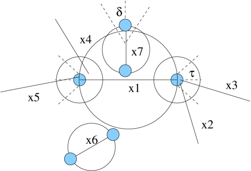
Figure 1: Connection and alignment interaction between segments. The circle around a segment represents the rejection region, whereas the circles around its extremities indicate the connection region. The values $\tau$ and $\delta$ are the curvature values allowing segments to align and to cross, respectively.

In Fig. 1 we show an example of a configuration of segments. The free segments are $x_{2},x_{4},x_{6}$ and $x_{7}$, this because the segment $x_{2}$ does not fullfil the orientation requirements for the connection and the others do not respect the connection condition. The segments $x_{3}$ and $x_{5}$ are singly connected, whereas the segment $x_{1}$ is doubly connected.

Similarly, the attraction region of a segment $\eta$ is the union of both circles centered at each extremity with a radius $r_{o}=l_{\eta}/4$. Two segments $\eta$ and $\zeta$ exhibit alignment interaction $\eta\sim_{o}\zeta$ if $d(k_{\eta},k_{\zeta})>\frac{1}{2}\max\{l_{\eta},l_{\zeta}\}$, if only one extremity of a segment is in the attraction region of the other segment, and if $\min\{\|\theta_{\eta}-\theta_{\zeta}\|,\pi-\|\theta_{\eta}-\theta_{\zeta}\|\}>\tau$, with $\tau$ a threshold value. The Candy model penalizes the segments having alignment interaction.

In the configuration shown in Fig. 1 $x_{3}\not\sim_{o}x_{1}$ and $x_{5}\not\sim_{o}x_{1}$, while the segments $x_{2}\sim_{o}x_{1}$ and $x_{4}\sim_{o}x_{1}$ because these pairs of segments exhibit high differences between their orientations.

Connectivity is a stronger interaction than alignment. Still, as we look for the filaments fitting the data in a random way, this last interaction gives us the possibility not to eliminate from the current configuration the segments with low data energy, which are almost connected.

Every segment $\eta$ is provided with a rejection region given by a circle centered in $k_{\eta}$ and of a radius $r_{r}=l_{\eta}/2$. Two segments $\eta$ and $\zeta$ exhibit rejection interaction if $d(k_{\eta},k_{\zeta})<\frac{l_{\eta}+l_{\zeta}}{2}$ and if $\|\|\theta_{\eta}-\theta_{\zeta}\|-\pi/2\|>\delta$, where $\delta$ is a threshold value. The Candy model forbids configurations containing rejecting (overlapping) segments.

If $d(k_{\eta},k_{\zeta})\leq\frac{1}{2}\max\{l_{\eta},l_{\zeta}\}$ and if $\|\|\theta_{\eta}-\theta_{\zeta}\|-\pi/2\|\leq\delta$, then the segments may cross or form a “T” junction. The configurations with crossing segments $\eta\sim_{x}\zeta$ are forbidden by the Candy model, whereas the “T” junctions are allowed.

Clearly, in Fig. 1 the segments $x_{1}$ and $x_{6}$ do not reject each other since they are far enough apart, while the segments $x_{1}$ and $x_{7}$ do not cross, forming a ”T” junction.

For any configuration of segments ${\bf x}=\{x_{1},\ldots,x_{n}\}$ with $i=1,\ldots,n$, we are able now to write for the probability density of the Candy model

$$\begin{array}[]{ccl}p_{r}({\bf x})&\propto&\left\{\prod_{i=1}^{n({\bf x})}\exp\left[\frac{l_{i}-l_{\max}}{l_{\max}}+\frac{w_{i}-w_{\max}}{w_{\max}}\right]\right\}\times\\ &&\gamma_{d}^{n_{d}({\bf x})}\gamma_{f}^{n_{f}({\bf x})}\gamma_{s}^{n_{s}({\bf x})}\gamma_{o}^{n_{o}({\bf x})}\times\\ &&\prod_{i<j}{\bf 1}\{x_{i}\not\sim_{r}x_{j}\}{\bf 1}\{x_{i}\not\sim_{x}x_{j}\}\end{array}$$ (5)

where $\gamma_{d},\gamma_{f},\gamma_{s}>0$ and $\gamma_{o}\in(0,1)$ are the model parameters, $n_{d}({\bf x}),n_{f}({\bf x}),n_{s}({\bf x})$ are the numbers of doubly, free and singly connected segments, and $n_{o}({\bf x})$ is the number of pairs of segments which are not well aligned. In order to avoid too many small segments in the configuration, the model favours segments covering a large area. Clearly the interaction energy is obtained taking $U_{r}({\bf x})=-\log p_{r}({\bf x})$.

With respect to the classical definition of the Candy model in van Lieshout & Stoica (2003a), the model described by Eq. (5) contains differences in the definition of interactions between segments. We kept the same name for our model, as we believe that the modifications required to apply it to cosmological data do not change the basic premises of the classical Candy model. Concerning connectivity, the present modifications were introduced in order to eliminate some “undesired” configurations, such as a segment being connected with itself or a segment being connected at one extremity with both extremities of another segment. Furthermore, the new modifications allow us to build more appropriate tailored moves for the Metropolis-Hastings dynamics simulating the model. The rejection region was extended, as the filaments we observe may be rather wide, hence we want to avoid overlapping of segments when the data are good enough. This is also the reason why the width penalty was introduced. Nevertheless, it is easy to prove that under these modifications, together with the one concerning the crossing interaction the Candy model is still locally stable and (Ripley-Kelly) Markovian (Ripley & Kelly 1977).

3.2 The data energy

The data energy checks whether a segment belongs to the network or not (Stoica 2001; Stoica et al. 2002, 2004). A segment $x$ is considered a part of the filament network, if its geometrical shape $\tilde{x}$ covers as many galaxies as possible. Still, we want to avoid the case where segments are found in a cloud of points rather than in a filament. Clouds of points can also be considered as inter-cluster filaments, but we want to favour the selection of the shoelace-like filaments, which are the more common morphological type (Colberg et al. 2004; Pimbblet & Drinkwater 2004), although other shapes (ribbons and sheets) can still be detected by the Candy model. To do this, we consider the shadow segments $x_{r}$ and and $x_{l}$ – the segments situated to the right and to the left of the segment $x$, as in Fig. 2. The above-mentioned case is avoided if the number of galaxies covered by $\tilde{x_{r}}$ and $\tilde{x_{l}}$ is small. Therefore, let us define the quantity $v_{{\bf y}}(x)$ given by

$$v_{{\bf y}}(x)=2n({\bf y}\cap\tilde{x})-n({\bf y}\cap\tilde{x_{r}})-n({\bf y}\cap\tilde{x_{l}}),$$ (6)

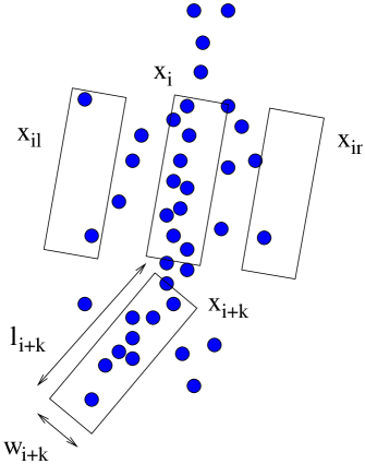
Figure 2: Locating segments in a pattern of points.

where $n({\bf y}\cap\tilde{x})$ is the number of galaxies covered by the geometrical shape of the segment $x$. Now, if the following three conditions: $v_{{\bf y}}(x)\geq 3$, $n({\bf y}\cap\tilde{x})>n({\bf y}\cap\tilde{x_{r}})$, and $n({\bf y}\cap\tilde{x})>n({\bf y}\cap\tilde{x_{l}})$ are simultaneously fulfilled, the data energy contribution of a segment is $V_{{\bf y}}(\{x\})=-v_{{\bf y}}(x)$. If one of the three conditions is not fulfilled then $V_{{\bf y}}(\{x\})=V_{\max}$, with $V_{\max}>0$ a positive fixed value.

The total data energy is defined as the sum of the data energy contributions of every segment in the configuration

$$U_{{\bf y}}({\bf x})=\sum_{x\in{\bf x}}V_{{\bf y}}(\{x\})$$ (7)

3.3 Simulation dynamics and optimization

The equations (5) and (7) provide us with all the ingredients needed to construct the Gibbs point process given by Eq. (3). The estimate of the network (Eq. 4) is obtained by means of a simulated annealing algorithm.

This algorithm iteratively samples the law $[p_{{\bf y}}({\bf x})]^{\frac{1}{T}}$ while slowly decreasing the temperature $T$. At high positive temperature values the state space is explored. When the temperature goes down to zero, $T\rightarrow 0$, the configurations of minimal energy are reached. A polynomial decreasing scheme $T_{k+1}=cT_{k}$ with $c\in[0.99,1.00]$ may be used for cooling.

For sampling from a probability density of a point process several Monte Carlo methods are available, such as the spatial birth-and-death process, the Metropolis-Hastings and reversible jumps dynamics, or the much more recent exact simulation techniques such as coupling from the past or clan of ancestors (Geyer & Møller 1994; Geyer 1999; Green 1995; Kendall & Møller 2000; van Lieshout 2000; van Lieshout & Stoica 2003b; Preston 1977). The Candy point process exhibits rather complicated interactions, hence the use of the spatial birth-and-death process or the cited exact simulation techniques are useful in practice only for a limited range of the model parameters. Therefore, for our present model we opted for a sampling algorithm based on the Metropolis-Hastings dynamics. Details concerning the implementation of samplers for the Candy model based on Metropolis-Hastings or reversible jumps processes can be found in van Lieshout & Stoica (2003a); Stoica (2001); Stoica et al. (2002, 2004).

4 Data

Figure 3: The spectral density used for the 2-D simulation ($P_{2}$), the corresponding spectral density for the 3-D case ($P_{3}$), and the spectral energy per unit logarithmic wavenumber interval $\Delta^{2}$, versus the wavenumber $k$.

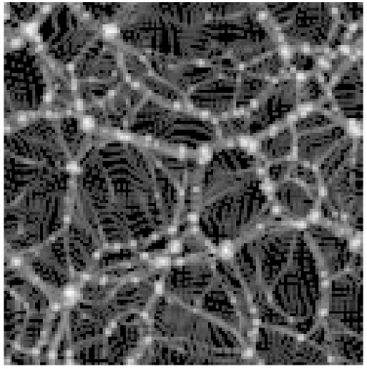
Figure 4: Dark matter density (logarithmic scale) for the data set B.

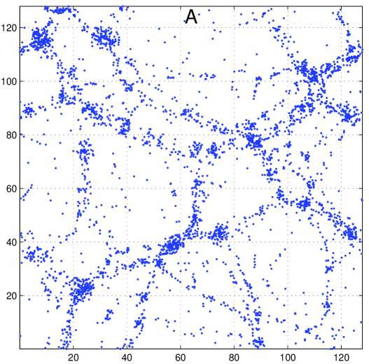
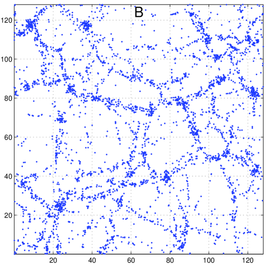
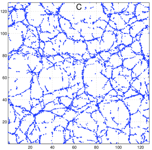
Figure 5: The simulated galaxy distribution for the three sets of data. Panel B corresponds to the dark matter distribution shown in Fig. 4. In this and the following figures the units of distance are $h^{-1}$Mpc, though in a 2-D world.

Table 1: Parameters of the data sets: $a$ is the cosmological expansion factor, $n$ is the number of galaxies, $\alpha$ is the void density threshold and $\beta$ is the biasing amplitude.

Case	$a$	$n$	$\alpha$	$\beta$
A	1.0	4127	0.5	0.20
B	0.6	4249	0.5	0.18
C	0.2	8879	1.0	0.49

The Candy process and its applications have been developed for 2-D maps. So the natural way to introduce them in cosmology is to consider 2-D cases, also. This will allow us to compare the results, and will make it easier to understand the problems arising. Our final goal is to apply the Candy process to describe 3-D networks of filaments, as the large-scale structure maps fill the space. The 3-D network consists of complete filaments, as do the 2-D geographical road maps, so the filaments in the test data should also be complete.

The observational galaxy maps showing filaments mainly have the geometry of a thin slice. Although such data have been used to study the large-scale filamentary structure, the slices do not provide proper data for that. The thickness of these slices is much smaller than the typical size of a filament, and although the maps give a visual impression of filaments, the filaments we see are pieces of real filaments, obtained by planar cuts through the real 3-D structure.

Another possibility is to use thicker slices, which can be selected, e.g., from the only large-scale contiguous data set for the moment, the 2dF survey (Colless et al. 2003). But this choice carries its own difficulties – thick slices give us the 2-D projection of the 3-D network, smearing essential details.

Simulations of the formation and evolution of large-scale structure can also provide us with galaxy maps. As a demonstration that we understand the basic features of the process, these maps show filamentary structure. How and why an initial Gaussian random density field develops filaments under self-gravitation is well explained by Bond et al. (1996).

The usual simulations give us 3-D universes, but it is easy to also simulate the evolution of structure in a 2-D universe. This has been done before, to obtain better numerical resolution (see, e.g., Beacom et al. 1991); we used 2-D simulations to get complete cosmological networks of model galaxies.

The present-day large-scale structure is determined, first, by the expansion history of the cosmological model, and, second, by the initial density and velocity fields at the start of the simulation. We chose the standard ’concordance’ cosmological model (Tegmark et al. 2001) to describe the expansion. As the initial fields are assumed to be Gaussian random fields, they are described by their power spectra (the spectral density of the density perturbations $P(k)$, where $k$ is the module of the wave-vector; see, e.g., Martínez & Saar 2002). We chose a simple expression for the spectral density that describes reasonably well the Cold Dark Matter (CDM) model (Jenkins et al. 1998) and modified it to get the same spectral energy contribution to the variance per unit logarithmic wavenumber interval, $\Delta^{2}(k)$, in our 2-D universe as in the real 3-D universe. In a 3-D universe this quantity is defined as

$$\Delta^{2}_{3}(k)=\frac{1}{2\pi^{2}}P_{3}(k)k^{3},$$

and in a 2-D universe as

$$\Delta^{2}_{2}(k)=\frac{1}{2\pi}P_{2}(k)k^{2};$$

the equality of the above quantities gives

$$P_{2}(k)=\frac{k}{\pi}P_{3}(k)$$

(the lower indices show the dimensionality of the space). This is the spectral density we used, with $P_{3}(k)$ taken from Jenkins et al. (1998). Both the spectral densities and the spectral energy used are shown in Fig. 3. As usual, the wavenumber is given in units of $h/\mbox{Mpc}$ where $h$ is the dimensionless Hubble parameter, the spectral densities are in units of Mpc${}^{3}/h^{3}$ ($P_{3}(k)$), Mpc${}^{2}/h^{2}$ ($P_{2}(k)$), and $\Delta^{2}(k)$ is dimensionless.

We selected the scales and spectrum amplitudes to get a picture similar to that we see in 3-D models (the size of the patch we modelled was $128h^{-1}$Mpc, and we used a $256^{2}$ grid with the same number of cold dark matter particles). These numbers are not really important, as this is a mock model, anyway. Then we ran a 2-D dynamical $N$-body simulation, developing the initial perturbations into large-scale structures – the present-day density and velocity fields.

These density fields describe the dark matter content of the universe. Populating model universes with galaxies is a complex problem, but for our purposes simple recipes are sufficient. We used two well-known properties of the large-scale galaxy distribution. First, galaxies avoid large low-density regions, known as voids; we modeled this by selecting a density threshold $\alpha$ (all our densities are given in the units of the mean density). In regions with density lower than this threshold no galaxies were placed. Secondly, galaxy density is biased in respect to the dark matter density. We found that the model galaxy distribution best resembled the observational maps for a nonlinear biasing law:

$$\rho_{\mbox{\scriptsize gal}}=\beta\sqrt{\rho_{\mbox{\tiny CDM}}},\qquad\rho_{\mbox{\tiny CDM}}\geq\alpha.$$ (8)

We chose the amplitudes $\alpha$ and $\beta$ to produce approximately the same number of galaxies as observed in cosmological slices of similar size.

Finally, we generated a realization of a Cox point process, using the galaxy density given by Eq. (8) as the driving probability. In order to see how well the Candy model works in different situations, we chose three different time moments from the simulation, with a different filamentary structure. As the earliest of them (our case C) has a very rich set of filaments, we generated about twice as many galaxies for that data set as for other sets. As usual in cosmology, we characterize the time moments by the value of the expansion factor $a$. This factor equals unity at the present epoch, and the earlier the epoch, the smaller is the expansion factor (our universe expands). The parameters for our three data sets are given in Table 1, and the dark matter density and galaxy distributions are compared for the set B in Fig. 4.

All the data sets are shown in Fig. 5.

4.1 Experimental results

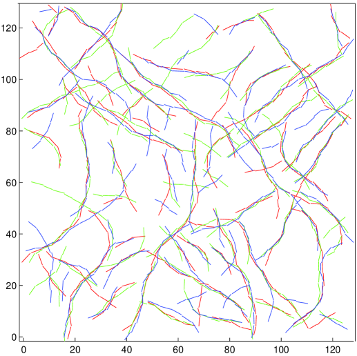
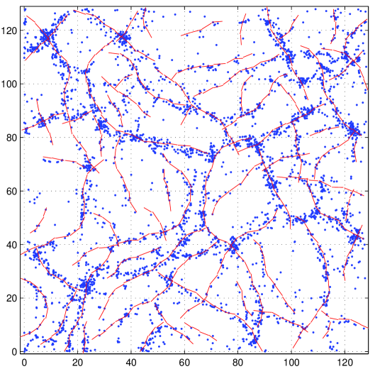
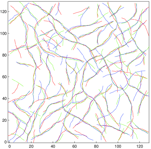
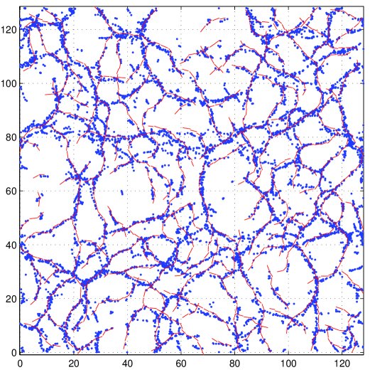
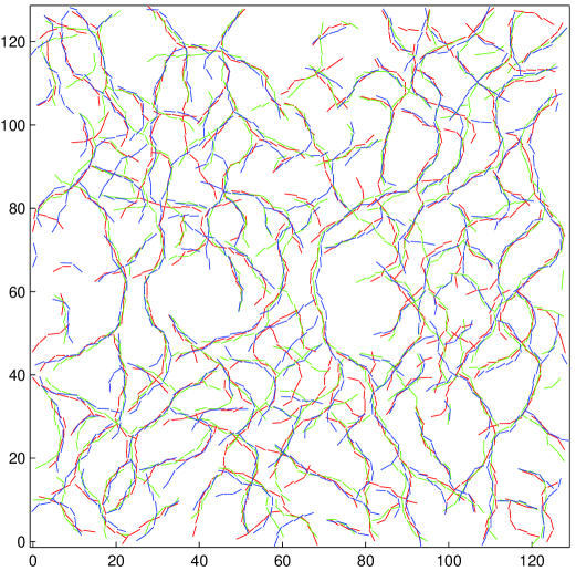
Figure 6: Results obtained for the three data sets: A (top row), B (middle row), and C (bottom row). The left panels show the “best network” extraction superposed on the data, the right panels show the three networks superposed. The networks for the first parameter set are shown by red curves, for set 2 by blue curves, and for set 3 by green curves.

Figure 7: Filament length distribution histograms for the three data sets (marked in the panels). Solid lines indicate parameter set 1, dashed lines set 2, and dotted lines set 3. The combined filament length distribution histograms for the three data sets is shown in the bottom right panel. Solid line indicates data set A, dashed line set B, and dotted line set C.

Table 2: The interaction parameters.

	Sets
Parameters	1	2	3
$-\log\gamma_{d}$	$-10$	$-10$	$-10$
$-\log\gamma_{f}$	8	7	7
$-\log\gamma_{s}$	2	2	1
$-\log\gamma_{o}$	3	3	3
$\quad V_{\max}$	25	25	25

A simulated annealing algorithm was implemented based on Metropolis-Hastings dynamics. The parameter for the cooling scheme was taken as $c=0.9995$ and the initial temperature was set to $10$. The algorithm was run for $10^{7}$ iterations, and the temperature was lowered every $10^{3}$ steps.

The Candy model has a large number of parameters, and these should be chosen carefully in order to get a good representation of the filaments in the data. The segment parameters (segment lengths and widths) have to be chosen such that the model filaments follow those in the data. Thus, for the first two data sets, the segment parameters were $l_{\min}=3,l_{\max}=5,w_{\min}=1,w_{\max}=2$; for the third data set, smaller segments were considered: $l_{\min}=2,l_{\max}=3,w_{\min}=0.95,w_{\max}=1.05$ (all distances are given in $h^{-1}$ Mpc). The interaction regions were defined by choosing the radius of the connecting region $r_{c}=0.5$ and the rejection parameter that forbids segments to cross, $\delta=0.1$ radians. The orientation parameter, which limits the local curvature of filaments, was chosen to be $\tau=0.5$ radians for the first two data sets and to be $\tau=0.75$ radians for the data set C.

We experimented with a large number of interaction parameters. Here we show the results for the three sets; they give almost equally good results. The interaction parameters for these sets are given in Table 2. The optimization method was run for each data set. High potentials were given to undesired configurations such as single and free segments, badly aligned pairs of segments with respect to the parameter $\tau$, and badly placed segments with respect to the data term.

The best filament network and the comparison between the three networks for each set of data is shown in Fig. 6. Note that we do not use the periodicity of the data — although numerical simulations are mostly periodic, the real galaxy distribution is not. Thus there is no sense in complicating the numerical procedure.

The best set of parameters for data set A was set 1. Examining the top row of Fig. 6 we see that the procedure works well. All obvious filaments that one would draw by eye are found, and the placement of “secondary” filaments in more sparsely populated regions is also good. Note also that galaxy concentrations (“clusters”) do not destroy the filamentary pattern; filaments usually branch in these regions.

The difference between the sets is slight, all parameter sets represent the network fairly well. All strong filaments coincide, the difference is in the small and weak filaments, built on a few points only. This is well seen in the right panel, where all three networks are superposed. Parameter set 2, for instance, generates spurious filaments in the sparsely populated upper central region of the point distribution, and set 3 produces several very short isolated filaments. On the other hand, it also provides a perfect branching point at $x=90,\,y=30$, which sets 1 and 2 do not find.

The middle row of Fig. 6 illustrates the filament networks found for data set B. This data set has a richer and more uniform selection of filaments than set A. As these sets have approximately the same number of galaxies, individual filaments in set B are more sparse and harder to identify. Nevertheless, the method works well, especially for the parameter set 1, the best set; this network is shown in the middle left panel of Fig. 6. There are only a few questionable short filaments, e.g. around $x=70,\,y=120$ and $x=10,\,y=50$. Parameter set 2 generates considerably more short isolated filaments, which do not represent the data well, and the filaments for parameter set 3 tend to deviate in wrong directions.

Data set C has the richest set of filaments. These are shorter and not as pronounced as the filaments in the first two data sets — this is the way the large scale structure develops in the universe. The early structure that set C describes evolves by concentrating into larger and larger clusters and filaments; small-scale structure becomes weaker and disappears gradually. In order to apply the Candy model, we had to generate about twice as many galaxies for this set as for the other two. As shown in the bottom row of Fig. 6, our procedure delineates the filamentary network satisfactorily here, too, although probably the segments should have been even smaller. As seen in the bottom left panel for the best parameter set (set 1 in this case, too), segments sometimes jump from an obvious filament to another (e.g., at $x=47,\,y=20$); there is also a tendency to form short filaments for a collection of a few points, as at $x=7,\,y=60$ and $x=75,\,y=107$.

Parameter set 2 is in this case about as good as set 1; it misses a few obvious filaments, however (e.g., at $x=124,\,y=50$), and has difficulties in resolving interaction regions (knots in the network), see the region at $x=70,\,y=110$. This region has been equally difficult to model for all three parameter sets. And, finally, parameter set 3 gives the worst filament placement among the three.

4.2 Length distribution

As the Candy model is able to reconstruct the filamentary network, given a point process (galaxy map), the collection of its parameters can be considered as a description of the network. When determined from the data by a likelihood procedure, they can serve as statistics of the network. But there are simple statistics we can already study; the simplest one is the probability distribution of the lengths of individual filaments (sets of connected segments). A similar problem, that of the length of the largest filament, has been addressed recently, using a pixel-based method to define filaments and finding the pixel size where the filaments are still statistically significant (Bharadwaj et al. 2004). As filaments delineate voids, the distribution of the lengths of filaments is also connected with the distribution of void sizes. This subject has a long history; see, e.g., Martínez & Saar (2002) and an interesting recent theoretical paper by Sheth & van de Weygaert (2004).

Comparison of the length histograms in Fig. 7 reveals a series of peaks, several distinct characteristic lengths in the filamentary network. These peaks are especially prominent for data sets A and C, and smeared out for set B. Also, the locations of the peaks do not depend much on the specific parameter set, the peaks more or less coincide. And although the sample sizes are a bit too small for the first two data sets to draw firm conclusions, inspection of the probability distributions shows that the peaks are real.

Another feature of the distributions is their pronounced tails – the lengths of filaments reach about 90, almost the full size of the box. Inspection of Fig. 6 shows that long filaments are those that pass through the branching points and are really collections of several filaments. So, in the future we have to find a recipe for locating the branching points and breaking the filaments; otherwise we shall lose connection with the void distribution. For the histograms in Fig. 7 this means that there would be additional contributions to the 20-40 length range, which are presently missing.

As the locations of the peaks are almost independent of the parameter set used, we combined the length data for the three parameter sets. These distributions for the three data sets are compared in the bottom right panel of Fig. 7. Thus these peaks are significant, revealing discrete scales in the data. We also see that the overall length distribution is shifted to the shorter sizes for set C, compared with A and B.

5 Other approaches

Figure 8: A Candy model (left panel) and the minimal spanning tree (right panel) for the same set of data (set A)).

There exist only a few methods to describe the observed filamentary network of galaxies. The best known approach is that of minimal spanning trees (MST) (Barrow et al. 1985). The minimal spanning tree connects all data points, and its length distribution function describes mainly the nearest-neighbour distance distributions, not the large-scale network we see. The MST also has to connect all points in the clusters, while the Candy model can be tuned to ignore them (as we have seen, clusters usually become branching points of the filament network in the Candy model). The differences between the MST and the Candy model can be well seen in Fig. 8. Nevertheless, the MST has been used extensively to describe the filamentary network; as the Candy model looks much better and is well suited for incomplete samples, it should lead to a better description of the cosmic filaments.

Using a technique based on multiscale geometric analysis Arias-Castro et al. (2003) have showed how filaments can be detected when they are embedded in a uniformly distributed background of points. This algorithm is specially aimed at finding hidden filamentary patterns in images or nearly Poissonian point processes. Our approach is different and is better suited for finding many filaments in clustered point processes, because the Candy model produces smoother maps and is able to better combine both local and large scale characteristics of the galaxy distribution.

Another, more recent approach to describing filaments (Bharadwaj et al. 2004) proceeds by binning the map (calculating a density field), and using Minkowski functionals of the isodensity contours to estimate the filamentarity of the objects. While this approach will classify all objects, it has two free parameters, the smoothing length (size of the density bin), and the isodensity level. True, in some respects our approach is similar to that, as the segments of the Candy model have a finite width (we are also estimating a density field). But our density estimator is anisotropic and adaptive, in principle, and we trace only filamentary structures.

A third approach that is also based on a density field, is to determine the saddle points and to build a network of field lines (directed along the gradient of the field), connecting saddle points with local maxima – the skeleton (Novikov et al. 2003). This approach could reconstruct well the cellular network of filaments (so far it has been applied to studying the pixelized cosmic microwave background data by Eriksen et al. 2004), but it will also depend on the density estimation procedure. And, as the authors say, this approach is computationally complex.

6 Conclusion and perspectives

The parameter values for our method were chosen by trial and error. Under these circumstances, parameter estimation using Monte Carlo maximum likelihood methods may be considered (Geyer 1999; van Lieshout & Stoica 2003a). These parameters could then be considered as statistics describing the filamentary network. They will certainly be much better suited for this task than the moments of the density distribution in real or in Fourier space which are commonly used in cosmology.

The data term is a very simple test. Much more sophisticated techniques such as testing the alignment of the points covered by a segment, or statistical tests such as the complete randomness test need investigation.

To our knowledge there is no proof for the existence of an optimal cooling scheme when using Metropolis-Hastings dynamics for simulating point processes in a simulated annealing algorithm. There is such a proof for the spatial birth-and-death process, but in practice the authors sample the model using a fixed cold temperature (van Lieshout 1994). The choice we opted for, a slow polynomial decreasing scheme, does not guarantee that the global optimum is reached.

But overall, as we have seen, the results are good, the Candy model can be tuned to trace the filamentary network well. And it can be naturally generalized to describe the real 3-D filamentary networks of galaxy maps; see Gregori et al. (2004). As we already said above, it can also be considered as a tool for providing statistics of filamentary networks. These are the future directions of our work.

7 Acknowledgements

We thank the referee Kevin Pimbblet for interesting comments that improved the paper. Enn Saar and Radu Stoica want to thank the Observatori Astronòmic de la Universitat de València where part of this work was done for its hospitality. This work has been supported by Valencia University through a visiting professorship for Enn Saar, by the Spanish MCyT project AYA2003-08739-C02-01 (including FEDER), by the Generalitat Valenciana project GRUPOS03/170, and by the Estonian Science Foundation grant 4695. We thank Rien van de Weygaert for his code to calculate the MST. The work of Jorge Mateu and Radu Stoica was carried out, respectively, under the grants BFM2001-3286 of the Spanish MCyT and SB2001-0130 from MECD.

References

- Arias-Castro et al. (2003) Arias-Castro, E., Donoho, D., & Huo, X. 2003, Adaptive multiscale detection of filamentary structures embedded in uniform random points, Technical report, Stanford University
- Barrow et al. (1985) Barrow, J. D., Sonoda, D. H., & Bhavsar, S. P. 1985, MNRAS, 216, 17
- Beacom et al. (1991) Beacom, J. F., Dominik, K. G., Melott, A. L., Perkins, S. P., & Shandarin, S. F. 1991, ApJ, 372, 351
- Bharadwaj et al. (2004) Bharadwaj, S., Bhavsar, S. P., & Sheth, J. V. 2004, ApJ, 606, 25
- Bond et al. (1996) Bond, J. R., Kofman, L., & Pogosyan, D. 1996, Nat, 380, 603
- Colberg et al. (2004) Colberg, J. M., Krughoff, K. S., & Connolly, A. J. 2004, astro-ph/0406665
- Colless et al. (2003) Colless, M., Peterson, B. A., Jackson, C., et al. 2003, astro-ph/0306581
- Cross et al. (2004) Cross, N. J. G., Driver, S. P., Liske, J., et al. 2004, MNRAS, 349, 576
- Dietrich et al. (2004) Dietrich, J. P., Schneider, P., Clowe, D., Romano-Diaz, E., & Kerp, J. 2004, astro-ph/0406541
- Ebeling et al. (2004) Ebeling, H., Barrett, E., & Donovan, D. 2004, ApJ, 609, L49
- Eriksen et al. (2004) Eriksen, H. K., Novikov, D. I., Lilje, P. B., Banday, A. J., & Górski, K. M. 2004, ApJ, 612, 64
- Geyer (1999) Geyer, C. J. 1999, in Stochastic geometry, likelihood and computation, ed. O. Barndorff-Nielsen, W. S. Kendall, & M. N. M. van Lieshout (CRC Press/Chapman and Hall, Boca Raton)
- Geyer & Møller (1994) Geyer, C. J. & Møller, J. 1994, Scan. J. Stat., 21, 359
- Gray et al. (2002) Gray, M. E., Taylor, A. N., Meisenheimer, K., et al. 2002, ApJ, 568, 141
- Green (1995) Green, P. 1995, Biometrika, 82, 711
- Gregori et al. (2004) Gregori, P., Mateu, J., & Stoica, R. S. 2004, in Spatial point process modelling and its applications, ed. A. Baddeley, P. Gregori, J. Mateu, R. S. Stoica, & D.Stoyan (Publicacions de la Universitat Jaume I, Castellon)
- Jenkins et al. (1998) Jenkins, A., Frenk, C. S., Pearce, F. R., et al. 1998, ApJ, 499, 20
- Kendall & Møller (2000) Kendall, W. S. & Møller, J. 2000, Adv. Appl. Prob., 32, 844
- Lacoste et al. (2002) Lacoste, C., Descombes, X., & Zerubia, J. 2002, A comparative ctudy of point processes for line network extraction in remote sensing, Research report 4516, INRIA Sophia-Antipolis
- Martínez & Saar (2002) Martínez, V. J. & Saar, E. 2002, Statistics of the Galaxy Distribution (Chapman & Hall/CRC, Boca Raton)
- Novikov et al. (2003) Novikov, D., Colombi, S., , & Doré, O. 2003, astro-ph/0307003
- Pimbblet & Drinkwater (2004) Pimbblet, K. A. & Drinkwater, M. J. 2004, MNRAS, 347, 137
- Pimbblet et al. (2004) Pimbblet, K. A., Drinkwater, M. J., & Hawkrigg, M. C. 2004, MNRAS, 354, L61
- Pimbblet et al. (2001) Pimbblet, K. A., Smail, I., Edge, A. C., et al. 2001, MNRAS, 327, 588
- Preston (1977) Preston, C. J. 1977, Bull. Int. Stat. Inst., 46, 371
- Reiss (1993) Reiss, R. D. 1993, A course on point processes (Springer-Verlag, New York)
- Ripley & Kelly (1977) Ripley, B. D. & Kelly, F. P. 1977, J. London Math. Soc., 15, 188
- Ruelle (1969) Ruelle, D. 1969, Statistical mechanics (Wiley, New York)
- Sheth & van de Weygaert (2004) Sheth, R. K. & van de Weygaert, R. 2004, MNRAS, 350, 517
- Stoica et al. (2004) Stoica, R., Descombes, X., & Zerubia, J. 2004, Int. J. Computer Vision, 57(2), 121
- Stoica (2001) Stoica, R. S. 2001, PhD thesis, Nice Sophia-Antipolis University
- Stoica et al. (2002) Stoica, R. S., Descombes, X., van Lieshout, M. N. M., & Zerubia, J. 2002, in Spatial statistics through applications, ed. J. Mateu & F. Montes (WIT Press, Southampton, UK)
- Tegmark et al. (2001) Tegmark, M., Zaldarriaga, M., & Hamilton, A. J. S. 2001, Phys. Rev. D, 63, 043007
- van Lieshout (1994) van Lieshout, M. N. M. 1994, Adv. Appl. Prob., 26, 281
- van Lieshout (2000) van Lieshout, M. N. M. 2000, Markov point processes and their applications (Imperial College Press/World Scientific Publishing, London/Singapore)
- van Lieshout & Stoica (2003a) van Lieshout, M. N. M. & Stoica, R. S. 2003a, Stat. Neerlandica, 57, 1
- van Lieshout & Stoica (2003b) van Lieshout, M. N. M. & Stoica, R. S. 2003b, Perfect simulation for marked point processes, Research report PNA-0306, CWI