A 1200$\mu$m MAMBO survey of ELAIS N2 and the Lockman Hole: I. Maps, sources and number counts

Abstract

We present a deep, new 1200$\mu$m survey of the ELAIS N2 and Lockman Hole fields using the Max Planck Millimeter Bolometer array (MAMBO). The areas surveyed are 160 arcmin² in ELAIS N2 and 197 arcmin² in the Lockman Hole, covering the entire SCUBA ‘8 mJy Survey’. In total, 27 (44) sources have been detected at a significance $\geq$4.0$\sigma$ ($\geq$3.5$\sigma$). The primary goals of the survey were to investigate the reliability of (sub)millimetre galaxy (SMG) samples, to analyse SMGs using flux ratios sensitive to redshift at $z\rm>3$, and to search for ‘SCUBA drop-outs’, i.e. galaxies at $z\rm>>3$. We present the 1200$\mu$m number counts and find evidence of a fall at bright flux levels. Employing parametric models for the evolution of the local 60$\mu$m IRAS luminosity function (LF), we are able to account simultaneously for the 1200 and 850$\mu$m counts, suggesting that the MAMBO and SCUBA sources trace the same underlying population of high-redshift, dust-enshrouded galaxies. From a nearest-neighbour clustering analysis we find tentative evidence that the most significant MAMBO sources come in pairs, typically separated by $\sim$23^′′. Our MAMBO observations unambiguously confirm around half of the SCUBA sources. In a robust sub-sample of 13 SMGs detected by both MAMBO and SCUBA at a significance $\geq$3.5$\sigma$, only one has no radio counterpart. Furthermore, the distribution of 850/1200$\mu$m flux density ratios for this sub-sample is consistent with the spectroscopic redshift distribution of radio-detected SMGs (Chapman et al. 2003). Finally, we have searched for evidence of a high-redshift tail of SMGs amongst the 18 MAMBO sources which are not detected by SCUBA. While we cannot rule out that some of them are SCUBA drop-outs at $z>>\rm 3$, their overall 850-to-1200$\mu$m flux distribution is statistically indistinguishable from that of the 13 SMGS which were robustly identified by both MAMBO and SCUBA.

1 Introduction

In a time of ‘high-precision cosmology’ one of the fundamental questions about which we remain largely ignorant is the formation and evolution of galaxies and clusters of galaxies. One of the most important breakthroughs in this field was the discovery of a significant population of far-IR-luminous, high-redshift sources in surveys at submillimetre (submm) and millimetre (mm) wavelengths using SCUBA and MAMBO (Smail, Ivison & Blain 1997; Hughes et al. 1998; Barger et al. 1999; Eales et al. 2000; Bertoldi et al. 2000), resolving at least half of the far-IR/submm background detected by the DIRBE and FIRAS experiments (e.g. Hauser et al. 1998).

It is widely believed that the large far-IR luminosities ($\mathrel{\raise 1.50696pt\hbox{$\scriptstyle>$}\kern-6.00006pt\lower 1.72218pt\hbox{{$\scriptstyle\sim$}}}$10${}^{12}\,\mbox{L${}_{\odot}\,$}$) of these sources is caused by intense UV light from starbursts and/or active galactic nuclei (AGN) being absorbed by dust and re-radiated longwards of $100$$\mu$m . The negative $k$-correction at $\lambda\geq 400$$\mu$m allows submm/mm observations to select star-forming galaxies at $z>1$ in an almost distance-independent manner, providing an efficient method of finding obscured, star-forming galaxies at 1 $<z<$ 10 (Blain & Longair 1993).

The large star-formation rates ($\sim$1000 $\mbox{M${}_{\odot}\,$}\,\mbox{yr}^{-1}$) found for (sub)mm galaxies (hereafter SMGs) are sufficient to construct a giant elliptical ($\sim$10${}^{11}\,\mbox{M${}_{\odot}\,$}$) in less than a Gyr, providing that the starburst is continuously fueled. This has led people to speculate that SMGs could be the progenitors of such galaxies (e.g. Dunlop 2001), a scenario which is further strengthened by the fact that the co-moving number density of SMGs appears to be consistent with that of today’s massive ellipticals (Scott et al. 2002; Dunne, Eales & Edmunds 2003). However, the nature of SMGs, and in particular their relationship with possible present-day counterparts, is not known, just as their relation to other high-redshift populations such as Lyman-break galaxies (LBGs) and extremely red objects (EROs) is not well understood.

Progress has been hampered by the large positional uncertainties of the SMGs. The relatively large beams of (sub)mm telescopes (11–14^′′, fwhm) makes it impossible to reliably tie an SMG to an optical or near-IR counterpart, unless additional data at a complementary wavelength are available. Since a characteristic feature of both starburst galaxies and AGN is radio emission, deep radio imaging has proven to be a highly efficient way of accurately identifying optical/near-IR counterparts to SMGs (Ivison et al. 1998, 2000, 2002; Smail et al. 2000).

Use of the radio-to-submm spectral index as an redshift indicator (Hughes et al. 1998; Carilli & Yun 1999, 2000) has shown that the SMGs lie at high redshift, with an estimated median redshift of $\geq 2$ (Ivison et al. 2002). Recently, Chapman et al. (2003, 2004) have obtained spectroscopic redshifts for $\sim$90 SMGs and found they span 0.8 $<z<$ 4, with a median of 2.4, although they cautioned that the distribution might be skewed towards lower redshifts since a requirement for getting a spectrum was that the SMGs had $\mu$Jy counterparts in the radio.

In a very deep radio survey of the Lockman Hole and ELAIS N2 fields, Ivison et al. (2002) found that about one third of SMGs did not have radio counterparts. One plausible explanation was that some of these radio-blank SMGs lie at very high redshifts. Such a population of SMGs — the so-called ‘high-redshift tail’ — would ask difficult questions of popular hierarchical models. The high-redshift SMGs would have low $S_{850\mu\rm{m}}/S_{1200\mu\rm{m}}$ flux ratios (see Eales et al. 2003) and would be readily detectable with MAMBO.

Blain, Barnard & Chapman (2003), amongst others, have pointed out the limitations of photometric redshift techniques: the redshift is degenerate with the far-IR luminosity as parametrised by the dust temperature, $T_{\rm d}$. In principle, however, a comparison between the $850$, $1200$$\mu$m and 1.4-GHz flux densities allows us, in some cases at least, to break this degeneracy, assuming that SMGs follow the radio/far-IR correlation. For example, an SMG which has a ’warm’ $S_{850\mu\rm{m}}/S_{1200\mu\rm{m}}$ ratio but has no radio counterpart is likely to be at high redshift. The $S_{850\mu\rm{m}}/S_{1200\mu\rm{m}}$ redshift estimator is particular sensitive at $z>\rm 3$ and is currently the most effective way to assess whether there is a significant high-redshift tail of SMGs.

The primary advantage of a mapping survey, rather than pointed photometry (on–off) observations of known sources (e.g. Eales et al. 2003), is that one obtains an unbiased view of the sky. Data are not skewed by the choice of targets, by possible errors in coordinates, or by potentially spurious assumptions about how the sky is expected to appear. A key goal of our new survey was to determine unbiased flux densities for the radio-blank SCUBA sources using MAMBO, and to search for new populations of mm-bright sources, in particular a sign of a dusty, star-forming $z\rm>>5$ population — ‘SCUBA drop-outs’ — that would be expected to be below the typical SCUBA detection threshold at $850$$\mu$m but detectable by MAMBO at $1200$$\mu$m .

In this paper we present a new, unbiased $1200$$\mu$m survey, using MAMBO on the IRAM 30m telescope, of the Lockman Hole and ELAIS N2, the two regions observed by the SCUBA 8 mJy survey (Scott et al. 2002; Fox et al. 2002). A plethora of multi-wavelength observations exist for both fields, including very deep X-ray, optical, near-IR, mid-IR and radio imaging (Hasinger et al. 2001; Manners et al. 2002; Ivison et al. 2002; Almaini et al. 2002). Our observations, data reduction and maps are described in §2 and 3. The source extraction technique and the source catalogues for each field are presented in §4, as are the results of Monte Carlo simulations to assess completeness, positional accuracy, flux boosting, etc. In §5 and 6 we present our measurements of the source counts and the clustering properties of MAMBO sources. Finally, §7 describes our joint analysis of the $850$ and $1200$$\mu$m samples, and implications for ongoing (sub)mm surveys and for the redshift distribution of SMGs.

Throughout, we have adopted a flat cosmology, with $\Omega_{m}=0.3$, $\Omega_{\Lambda}=0.7$ and $H_{0}=70$ km ${\rm s^{-1}}$ Mpc^-1.

2 Observations

The survey was carried out with the 37- and 117-channel MPIfR Max Planck Millimeter Bolometer arrays (MAMBO-I and MAMBO-II; Kreysa et al. 1998) at the IRAM 30m telescope on Pico Veleta near Granada in Spain. Both MAMBO-I and MAMBO-II are He³-cooled arrays operating at an effective frequency of 250 GHz or $1200$$\mu$m with a half-power spectral bandwidth of 80 GHz. At $1200$$\,\mu$m, the 30m telescope has an effective beam of 10.7^′′ (fwhm). The arrays are background limited and the performance of the array routinely gives noise equivalent flux densities (NEFDs) of 30 – 45 mJy Hz^-1/2. The bolometer feedhorns are arranged in a compact hexagonal pattern each with a diameter of $2F\lambda$ which ensures an optimal coupling to the incoming radiation from a point source. MAMBO-II is amongst the largest (sub)mm bolometer arrays currently in use. In combination with the IRAM 30m dish which has a surface accuracy of 75 $\mu$m rms, it is the most powerful tool for large blank-field surveys at (sub)mm wavelengths, and will remain so until the advent of APEX/LABOCA, JCMT/SCUBA2 and LMT/Bolocam.

Scan-mapping along the azimuthal direction is the only method available at the 30m to map large areas of the sky. The signal from the sky is modulated by the secondary mirror (the wobbler) which is wobbling in the the scan direction (azimuth). The wobbler frequency is 2 Hz which reflects a compromise between wanting to eliminate changes in the atmosphere on as short a timescale as possible and the challenges involved in moving a 2m secondary at this frequency and keeping it mechanically stable. We used a standard on-the-fly MAMBO scan-map, typically $300\arcsec\times 320\arcsec$ in size, scanned at a velocity of 5^′′ s^-1, and with an elevation spacing between each subscan of 8^′′. Hence, a map consists of 41 subscans of 60s each. This results in a fully-sampled map over a $300\arcsec\times 320\arcsec$ region in $\sim$43 min (this includes $\sim 3$s of overhead per subscan). In order to obtain uniform coverage, a regular grid with a grid-spacing of 2$\arcmin$ was defined across each of the two fields. Each grid position was observed once which in practice means that, in the final map, each point on the sky has been observed at least two times. In principle, this ensures that an rms of $\sim$0.8 mJy beam^-1 is reached across most of the field. In practice, however, scans were taken in slightly different weather conditions which means that the noise is not entirely uniform. In order to eliminate any possible systematics and any residual effects from the double beam profile, wobbler throws in the range $36\mbox{${}^{\prime\prime}$}-45\mbox{${}^{\prime\prime}$}$ were used. Furthermore, maps were taken with different scan-directions, just as care was taken to map each grid position once while the field was rising and once while it was setting. All this served the purpose of minimising any systematic effects from the atmosphere and/or instrument which may otherwise had arisen from observing the same grid-position in two consecutive maps using identical wobbler- and scan-configuration.

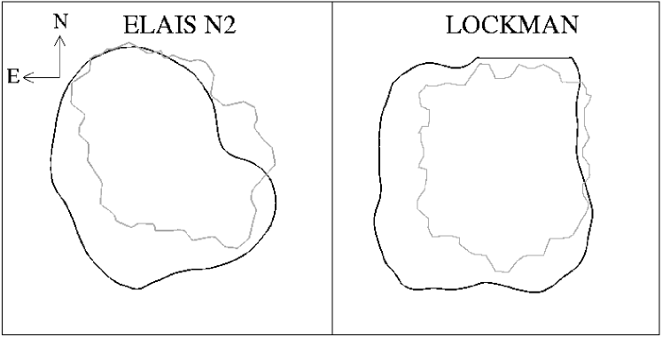
Figure 1: The MAMBO survey regions (outlined in black) of the ELAIS N2 and Lockman Hole fields. The mapped areas are 160 and 197 sq. arcmin in ELAIS N2 and Lockman Hole, respectively. For comparison, the coverage of the SCUBA UK 8 mJy Survey (Scott et al. 2002) is also shown (grey curve). The boxes are $21\mbox{$\stackrel{{\scriptstyle\prime}}{{\textstyle.}}$}7\times 21\mbox{$\stackrel{{\scriptstyle\prime}}{{\textstyle.}}$}7$.

The two fields were only observed when above $30\mbox{${}^{o}$}$ and below $70\mbox{${}^{o}$}$ in elevation. The latter constraint, which avoids distorted scan-maps, was particularly troublesome for the ELAIS N2 field which reaches a maximum elevation of $85\mbox{${}^{o}$}$ at Pico Veleta.

Since observations were pooled, they were done only under good weather conditions, i.e.  when the atmospheric zenith opacity at $1200$$\mu$m was less than 0.3, with low sky-background variations. After each map, i.e. every hour, the telescope was pointed and focused. The opacity of the atmosphere was measured every other hour by doing a skydip but was also continuously monitored with a radiometer located next to the telescope. Variations in the sky-background were monitored from the pointings by on-line measurements of the correlation of the horns across the array. Also quick on-offs of the pointing sources were done throughout the night in order to check the sky noise and calibration. In order to tie down the absolute flux calibration, primary flux calibrators (including planets when available) were observed at the beginning and end of each run, and resulted in an absolute flux calibration of better than 20 per cent.

In total, 34 scan-maps, corresponding to 26 hrs, went into the final map of ELAIS N2, all of which were obtained with MAMBO-II as part of the pooled observing mode during the winter period of the 2001-2002 and 2002-2003 seasons. The bulk of the observations of the Lockman Hole were also obtained during that time using MAMBO-II, although, early observations of the Lockman Hole during the winter of 2000–01, and to some extent also 2001–02, were obtained with the 37-channel MAMBO-I array. For the Lockman Hole, 19 and 51 scan-maps taken with MAMBO-I and MAMBO-II, respectively, were used for the final map, equivalent to a total integration time of 53 hr.

The areas surveyed were 160 arcmin² in the ELAIS N2 field and 197 arcmin² in the Lockman Hole. In the case of ELAIS N2 the MAMBO observations were designed to cover the region observed at $850$$\mu$m as part of the SCUBA UK 8 mJy Survey (Scott et al. 2002). The small fraction of the SCUBA map which is not covered by our observations (Fig. 1) is also the most noisy, and no $850$$\mu$m sources were detected in that region. However, in the Lockman Hole the overlap between MAMBO and SCUBA observations is complete, as is seen from Fig. 1. The Lockman Hole MAMBO data presented in this paper are part of the larger area MAMBO Deep Field Survey (Bertoldi et al. 2000; Dannerbauer et al. 2002; Bertoldi et al. 2004, in prep.). In addition, the Lockman Hole is being targeted by SCUBA as part of the SCUBA Half Degree Extragalactic Survey (SHADES — http://www.roe.ac.uk/ifa/shades/), and the data presented here constitute only a small part of the area surveyed at (sub)mm wavelengths in that part of the sky.

3 Data reduction

The data were reduced using the mopsi software package (Zylka 1998). Bolometers which were either dead or very noisy were flagged from the data reduction, and the remaining data streams were de-spiked, flat-fielded and corrected for atmospheric opacity.

Since all bolometers look through the same region of the atmosphere at any given time, there will be a correlated signal across the array which will have to be removed in order to recover the (uncorrelated) astronomical signal. In mopsi the removal of this correlated sky background is done in an iterative way. For each bolometer an inner and outer radius from the channel is specified, and the correlation with every bolometer lying within this annulus is computed. In our case, we chose an inner and outer radius of 1^′′ and 60^′′, respectively, which is suitable for compact weak sources. The correlated signals of the surrounding 6 channels with the best correlation were then chosen and the average correlated noise subtracted from the bolometer in question. This procedure is then repeated until the sky background has been removed satisfactorily across the array.

Up until this point in the data reduction, the signal from each chopping position (called the on and off phase) was processed separately, the reason being that in a single phase the bolometers correlate much better which results in a much more reliable subtraction of the background. mopsi then calculated the phase difference, thereby effectively removing any electronic systematics between the data obtained in one wobbler position and the other. Additional de-spiking and baseline-fitting was then done on the phase differences, from which the weights for each bolometer were calculated.

Finally, the data were restored and rebinned using a shift-and-add technique which for each map produces a positive image bracketed by two negative images of half the intensity located one wobbler throw away. The rebinning was done onto a grid of 1 square arcsec pixels, with the flux in each pixel being a noise-weighted average of the bolometers hitting that position. mopsi also outputs a weight image, $W$, which at pixel position $(i,j)$ is given by $W(i,j)=\sum_{k}1/\sigma_{k}^{2}$, i.e. the error on the noise-weighted average, where $k$ denotes summing over the bolometers ’seen’ by pixel $(i,j)$.

The noise maps are shown in Figure 2. The rms noise in the deepest parts of the maps is $\sim$0.6 mJy beam^-1, increasing towards the edges. The Lockman Hole received more integration time than the ELAIS N2 field and as a result it is slightly deeper and has more uniform noise properties than the latter.

4 Source extraction and Monte Carlo Simulations

4.1 Source extraction

Scan-mapping is the only option for large area mapping at the IRAM 30m telescope, and as a result the chopping direction is not fixed on the sky but varies with time which means that the chops are smeared out in the final map. Hence, unlike SCUBA jiggle maps, one cannot utilise the extra information contained in the position of the negative side-lobes for source extraction. Instead, a simple matched-filtering technique was adopted, using a Gaussian as the filter. However, as is seen from the noise images shown in Figure 2, the noise is not entirely uniform across the two fields and any attempt at extracting sources has to take this into account. This was done by adopting a noise-weighted convolution technique similar to that of Serjeant et al. (2003). In order to account for the 10.7^′′ beam and the typical pointing error of 3^′′ rms, a Gaussian PSF, $P(x,y)$, with a fwhm of $\sqrt{10\mbox{$\stackrel{{\scriptstyle\prime\prime}}{{\textstyle.}}$}7^{2}+3\mbox{$\stackrel{{\scriptstyle\prime\prime}}{{\textstyle.}}$}0^{2}}=11.1\mbox{${}^{\prime\prime}$}$ was fitted to each pixel in the image $S(i,j)$ by minimising the following expression:

$$\chi^{2}(i,j)=\sum_{x,y}W(i-x,j-y)\left(S(i-x,j-y)-FP(x,y)\right)^{2}$$ (1)

where $W$ is the weight image which is related to the noise by $W=1/N^{2}$, and $F$ is the best-fit flux value to pixel $(i,j)$ and is given by:

$$F(i,j)=\frac{\sum_{x,y}S(i-x,j-y)W(i-x,j-y)P(x,y)}{\sum_{x,y}W(i-x,j-y)P(x,y)^{2}}.$$ (2)

The error on the flux can then be shown to be:

$$\Delta F(i,j)=\frac{1}{\sqrt{\sum_{x,y}W(i-x,y-j)P(x,y)^{2}}}.$$ (3)

The signal-to-noise images, $F/\Delta F$, obtained in this way are shown in Figure 3 and 4 for the ELAIS N2 field and Lockman Hole, respectively. The final source catalogues for ELAIS N2 and the Lockman Hole are listed in Table LABEL:table:source-list-n2 and LABEL:table:source-list-lh. We find a total of 13 sources at significance $\geq$$4.0\sigma$, and 21 sources with $\geq$$3.5\sigma$ in the ELAIS N2 region while the number of sources in the Lockman Hole are 14 and 23 at $\geq$$4.0\sigma$ and $\geq$$3.5\sigma$, respectively.

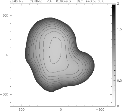
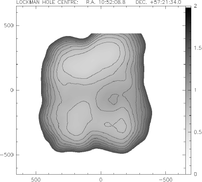
Figure 2: Noise maps of the ELAIS N2 and Lockman Hole East fields. Contours are at 0.7, 0.8 … 1.5 mJy beam^-1. The axes denote the offset (arcsec) from the map centre, and the intensity scale is in units of mJy beam^-1.

Table 1: $1200$$\mu$m MAMBO source catalogue in the ELAIS N2 field. The rms noise in the centre of the map is $\sim$0.65 mJy beam ^-1 and increases towards the edges. The area surveyed in the ELAIS N2 field is 160 arcmin ².

ID	MAMBO ID	RA (J2000)	Dec (J2000)	$S_{1200\mu\rm{m}}\pm\sigma_{1200\mu\rm{m}}$	$S/N$
$\sigma\geq 4.0$ Detections
MM J163647+4054	N2 1200.1	16:36:47.9	+40:54:46	$4.0\pm 0.8$	5.00
MM J163639+4053	N2 1200.2	16:36:39.1	+40:53:26	$5.0\pm 1.0$	5.00
MM J163635+4055	N2 1200.3	16:36:35.7	+40:55:59	$3.9\pm 0.8$	4.87
MM J163639+4056	N2 1200.4	16:36:39.1	+40:56:36	$3.4\pm 0.7$	4.85
MM J163632+4059	N2 1200.5	16:36:32.1	+40:59:46	$5.7\pm 1.2$	4.75
MM J163708+4054	N2 1200.6	16:37:08.3	+40:54:18	$4.2\pm 0.9$	4.66
MM J163640+4056	N2 1200.7	16:36:40.7	+40:56:46	$3.2\pm 0.7$	4.57
MM J163710+4055	N2 1200.8	16:37:10.5	+40:55:02	$4.0\pm 0.9$	4.44
MM J163705+4054	N2 1200.9	16:37:05.8	+40:54:26	$4.0\pm 0.9$	4.44
MM J163650+4057	N2 1200.10	16:36:50.3	+40:57:36	$3.1\pm 0.7$	4.42
MM J163656+4058	N2 1200.11	16:36:56.3	+40:58:14	$2.5\pm 0.6$	4.16
MM J163713+4054	N2 1200.12	16:37:13.8	+40:54:03	$4.9\pm 1.2$	4.08
MM J163619+4054	N2 1200.13	16:36:19.5	+40:54:00	$5.7\pm 1.4$	4.07
$4.0>\sigma\geq 3.5$ Detections
MM J163640+4058	N2 1200.14	16:36:40.4	+40:58:44	$3.1\pm 0.8$	3.87
MM J163636+4057	N2 1200.15	16:36:36.2	+40:57:19	$3.1\pm 0.8$	3.87
MM J163644+4102	N2 1200.16	16:36:44.8	+41:02:01	$2.7\pm 0.7$	3.85
MM J163706+4053	N2 1200.17	16:37:06.7	+40:53:15	$4.2\pm 1.1$	3.81
MM J163655+4059	N2 1200.18	16:36:55.9	+40:59:12	$2.2\pm 0.6$	3.66
MM J163658+4104	N2 1200.19	16:36:58.3	+41:04:37	$2.9\pm 0.8$	3.62
MM J163647+4055	N2 1200.20	16:36:47.9	+40:55:39	$2.5\pm 0.7$	3.57
MM J163715+4055	N2 1200.21	16:37:15.6	+40:55:40	$3.9\pm 1.1$	3.54

Table 2: $1200$$\mu$m MAMBO source catalogue in the Lockman Hole field. The rms noise is $\sim$0.6 mJy beam^-1 at the centre where the map is deepest, and increases towards the edges. The total area surveyed is 197 arcmin².

ID	MAMBO ID	RA (J2000)	Dec (J2000)	$S_{1200\mu\rm{m}}\pm\sigma_{1200\mu\rm{m}}$	$S/N$
$\sigma\geq 4.0$ Detections
MM J105238+5724	LE 1200.1	10:52:38.3	+57:24:37	$4.8\pm 0.6$	8.00
MM J105238+5723	LE 1200.2	10:52:38.8	+57:23:22	$4.1\pm 0.6$	6.83
MM J105204+5726	LE 1200.3	10:52:04.1	+57:26:58	$3.6\pm 0.6$	6.00
MM J105257+5721	LE 1200.4	10:52:57.0	+57:21:07	$5.7\pm 1.0$	5.70
MM J105201+5724	LE 1200.5	10:52:01.3	+57:24:48	$3.4\pm 0.6$	5.66
MM J105227+5725	LE 1200.6	10:52:27.5	+57:25:15	$2.8\pm 0.5$	5.60
MM J105204+5718	LE 1200.7	10:52:04.7	+57:18:12	$3.2\pm 0.7$	4.57
MM J105142+5719	LE 1200.8	10:51:42.0	+57:19:51	$4.1\pm 0.9$	4.55
MM J105227+5722	LE 1200.9	10:52:27.6	+57:22:20	$3.1\pm 0.7$	4.42
MM J105229+5722	LE 1200.10	10:52:29.9	+57:22:05	$2.9\pm 0.7$	4.14
MM J105158+5717	LE 1200.11	10:51:58.3	+57:17:53	$2.9\pm 0.7$	4.14
MM J105155+5723	LE 1200.12	10:51:55.5	+57:23:10	$3.3\pm 0.8$	4.12
MM J105246+5724	LE 1200.13	10:52:46.9	+57:24:47	$2.4\pm 0.6$	4.00
MM J105200+5724	LE 1200.14	10:52:00.0	+57:24:25	$2.4\pm 0.6$	4.00
$4.0>\sigma\geq 3.5$ Detections
MM J105245+5716	LE 1200.15	10:52:45.1	+57:16:05	$3.1\pm 0.8$	3.87
MM J105244+5728	LE 1200.16	10:52:44.8	+57:28:12	$5.0\pm 1.3$	3.84
MM J105121+5718	LE 1200.17	10:51:21.5	+57:18:40	$4.8\pm 1.3$	3.69
MM J105157+5728	LE 1200.18	10:51:57.7	+57:28:00	$2.2\pm 0.6$	3.66
MM J105128+5719	LE 1200.19	10:51:28.4	+57:19:47	$4.0\pm 1.1$	3.63
MM J105224+5724	LE 1200.20	10:52:24.4	+57:24:20	$1.8\pm 0.5$	3.60
MM J105131+5720	LE 1200.21	10:51:31.3	+57:20:06	$3.6\pm 1.0$	3.60
MM J105203+5715	LE 1200.22	10:52:03.0	+57:15:46	$2.8\pm 0.8$	3.50
MM J105223+5715	LE 1200.23	10:52:23.4	+57:15:27	$2.8\pm 0.8$	3.50

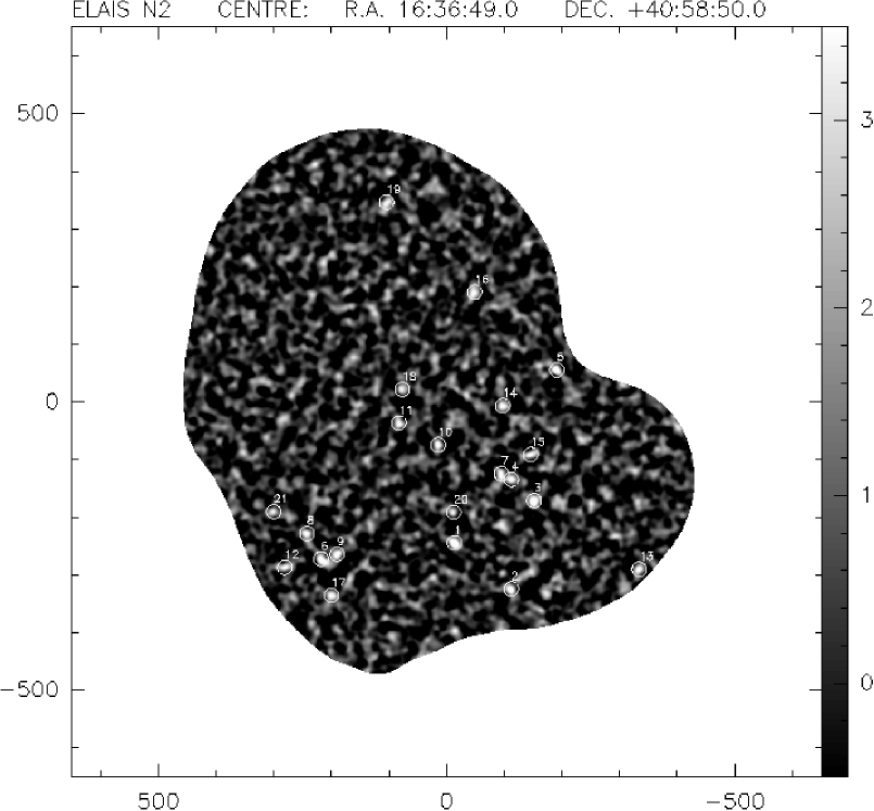
Figure 3: $1200$$\mu$m MAMBO signal-to-noise map of the ELAIS N2 field. Sources detected at $\geq$$3.5\sigma$ are circled in white, and are numbered in order of significance. The axes denote the offset (arcsec) from the map centre.

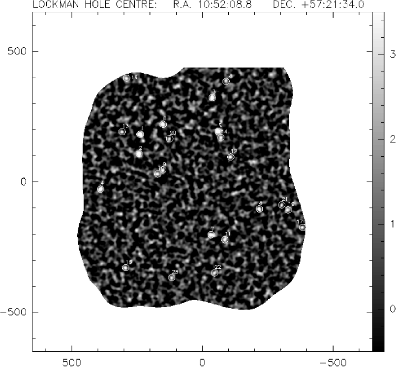
Figure 4: $1200$$\mu$m MAMBO signal-to-noise map of the Lockman Hole field. Sources detected at $\geq$$3.5\sigma$ are circled in white, and are numbered in order of significance. The axes denote the offset (arcsec) from the map centre.

4.2 Monte Carlo Simulations

Extensive Monte Carlo simulations were performed in order to determine the reliability of the source extraction technique, i.e. how large a fraction of the extracted sources are due to spurious noise peaks, and how well does the extraction reproduce fluxes and positions as a function of signal-to-noise? Due to the slight difference in survey depth and also geometry between the ELAIS N2 and Lockman Hole maps, we decided to perform separate Monte Carlo simulations for each of the two fields.

In order to assess the contamination from spurious noise peaks to the source catalogues, we produced maps based on the real data but with the astrometry corrupted. This was done by randomising the array parameters of each scan and then producing final maps using the same mopsi data reduction pipeline as for the real map. The advantage of this method is that the correlated noise in the raw data is preserved, and is taken out during the data reduction process in the same manner as for the real map. As a result, this method should give a realistic picture of the number of spurious noise peaks expected in our maps. We produced 100 such astrometrically corrupted maps and counted the number of positive spurious sources as a function of detection threshold. The results are shown in Figure 5 with empty and filled circles referring to the ELAIS N2 and Lockman Hole maps, respectively. As expected, the number of spurious detections drops off exponentially as a function of signal-to-noise threshold. From Figure 5 we find that a threshold of $4.0\sigma$ results in less than one spurious source expected at random, while a cut-off at $3.5\sigma$ yields less than 2 spurious sources per field. We adopt $3.5\sigma$ as the detection cut-off for sources in both fields since it provides a good compromise between catalogue size and source reliability.

Monte Carlo simulations were also used to test the completeness and reliability of the flux and position estimates. Sources in the flux range 1–12 mJy were added to the map in steps of 0.5 mJy, one at a time and each at a random position, with 50 sources in each flux bin. We used a scaled beam pattern as the template for the artificial sources. However, due to sky-rotation, the double-beam profile varies across the map and as a result a separate multi-beam PSF had to be constructed for each source, depending on its position in the map. To accomplish this, the source — with its correct intensity and position — was added to the data stream and then the data were reduced in the same manner as the real data. Thus, each artificial source added to the map had exactly the right multi-beam profile corresponding to its position in the map. Finally, sources were extracted using the same detection threshold as used for the real map. If a simulated source happened to fall within half a beam width of a real source in the map, it was discarded from the analysis. The results from these Monte Carlo simulations are shown in Figure 6, again with open and filled circles representing results based on the ELAIS N2 and Lockman Hole fields, respectively.

Figures 6a and b show the completeness of the survey, i.e. the percentage of recovered sources in our Monte Carlo simulations as a function of input flux density. As expected the source extraction does well in extracting all of the brighter sources, but fares less well for sources close to the detection threshold. In both fields the completeness is seen to be $\sim$50 per cent at a flux level of $\simeq$2.5 mJy, increasing to about 95 per cent at 3 mJy. The solid curves are best fits of the function $f(S_{in})=1-exp(A(S_{in}-B)^{C})$.

In Figures 6c and d we have plotted the ratio between the input and output fluxes $S_{out}/S_{in}$, as a function of the input flux density. It is seen that fainter sources tend to have higher extracted fluxes than brighter sources. This effect — ’flux boosting’ in Scott et al. (2002) — is due to the instrumental noise from the array itself and the confusion noise from faint sources below the detection threshold conspiring to scatter the retrieved fluxes upwards. As expected, flux boosting has the greatest impact at faint flux levels, where we find it can be as high as $\sim$30 per cent. However, for input fluxes $\geq$2 mJy the boosting is on average no more than $\sim$20 per cent, which is comparable to the calibration errors, see section 2. It is also comparable to the boosting factor reported by Eales et al. (2003) from a comparison of MAMBO fluxes obtained from a map and from photometry observations. An average flux boosting factor of $\sim$15 per cent was derived by Scott et al. (2002) from Monte Carlo simulations of their 8 mJy Survey. The solid lines in Figures 6c and d represent best fits to the data points of the function $f(S_{in})=1+Aexp(BS_{in}^{C})$.

The average positional offset between the input and output positions of the added sources is shown as a function of flux density in Figures 6e and f. Not surprisingly, the source extraction reproduces the true positions less well for faint sources than for brighter sources. It is seen that, in the flux range 2–5 mJy where most of our sources lie, the positional error is of the order 1.5–3.0^′′. This is slightly better than the 3–4^′′ errors typically quoted by SCUBA surveys (Webb et al. 2003; Scott et al. 2002; Borys et al. 2003) and may be due to the smaller MAMBO beam.

Figure 5: Expected average number of spurious positive sources in ELAIS N2 (empty circles) and the Lockman Hole (filled circles) as a function of signal-to-noise ratio. The solid and dashed lines are the expected number of positive spurious sources in the ELAIS N2 and Lockman Hole, assuming the noise is purely Gaussian and the MAMBO beam is a Gaussian with a fwhm of $10.7\mbox{${}^{\prime\prime}$}$.

Figure 6: Results from Monte Carlo simulations. The solid lines in all three panels represent best fits to the points, see text for details. As in Figure 5, empty and filled circles refer to results from the ELAIS N2 and Lockman Hole maps. Top: Percentage of added sources recovered against input flux in the range 1 to 12 mJy. Middle: The ’boosting’ factor, i.e. the factor by which the input flux is scattered upwards due to instrumental and confusion noise (Eddington bias), plotted against input flux. Bottom: Deviations between true (input) positions and the positions derived from the source extraction technique as a function of input flux.

5 Number counts of MAMBO sources

In order to derive the $1200$$\mu$m number counts we must correct the raw number counts for the effects of flux boosting and the fact that the survey is not complete at faint flux levels. Finally, we need to assess to what degree spurious sources contaminate the number counts.

Addressing the last issue first, it is seen from Figure 5 that at a detection threshold of $4.0\sigma$ we expect no spurious positive sources; at a threshold of $3.5\sigma$ we expect at most two. Furthermore, the flatness of the curves at $3.5\sigma$ implies that a slight error in the noise estimate will not change the number of false sources dramatically. This would not have been the case had we used a lower threshold of $3.0\sigma$. As a result, we have used the $\geq$$3.5\sigma$ catalogues to derive the number counts. While we cannot predict which flux bins the spurious sources will fall into, it is seen from Tables LABEL:table:source-list-n2 and LABEL:table:source-list-lh that the $\geq$$3.5\sigma$ sources span a wide range in flux. It is therefore unlikely that the spurious sources will be restricted to a single flux bin, and as a result their effect on the number counts is expected to be negligible.

Flux boosting was corrected for in a statistical way by applying the best-fit curves in Figures 6c and d to the raw output fluxes. The boost-corrected number counts obtained in this way were then corrected for completeness using the fitted completeness curves in Figures 6a and b.

The final integrated number counts in flux bins 2.75, 3.25, 3.75, 4.25, 4.75, and 5.25 mJy are given in Table LABEL:table:number-counts-table along with the raw number counts. The table shows the counts derived for the ELAIS N2 and Lockman Hole separately, as well as the combined number counts. The quoted errors correspond to the 95 per cent two-sided confidence level of a Poissonian distribution. The number counts derived from the two fields separately are seen to agree well within the error. In Figure 7 we have plotted the corrected accumulative $1200$$\mu$m number counts as derived from the MAMBO survey presented in this paper. While the surface density of SCUBA sources detected at $850$$\mu$m has been fairly well constrained over a large range in flux density thanks to a number of large submm surveys (Smail et al. 1997; Scott et al. 2002), only one other published MAMBO survey has so far attempted to constrain the $1200$$\mu$m number counts (Bertoldi et al. 2000).

For comparison we have also plotted the $850$$\mu$m source counts as derived from a number of SCUBA surveys. It is seen that the $1200$$\mu$m counts are lower than those at $850$$\,\mu$m. This is expected if one assumes that the MAMBO and SCUBA sources trace the same population of dust-enshrouded galaxies: the lower MAMBO counts are due to the fact that one is sampling further down the Rayleigh-Jeans tail than at $850$$\,\mu$m. Thus, if one scales the MAMBO fluxes by a factor of $\sim$2.5, which roughly corresponds to the $850/1200$$\mu$m flux ratio for a starburst at $z\sim\rm 2.5$, the MAMBO counts are found to coincide with the SCUBA counts. The overall similarity between the shape of the $1200$ and $850$$\mu$m number counts lends support to the view that the MAMBO and SCUBA sources are the same population viewed at slightly different wavelengths.

At flux levels fainter than $\sim$4 mJy the MAMBO counts display a power-law slope of $\alpha\simeq-2.2$, similar to that of the SCUBA counts in the flux range 2–9 mJy. The $1200$$\mu$m source counts appears to show a break at $\sim$4 mJy beyond which the slope of the counts steepens to $\alpha\sim-4.7$. The dot-dashed curve in Figure 7 represents a Schechter-type function of the form $dN/dS\propto(S/4\rm{mJy})^{-2.3}exp(-S/4\rm{mJy})$. The Schechter function has a natural break at 4 mJy and appears to provide a somewhat better match than a power law, although the data do not allow for a statistically significant distinction between a power law and a Schechter function. At the bright end of the $850$$\mu$m counts there is some disagreement between the SCUBA surveys, with the Scott et al. (2002) counts dropping off more steeply than found by Borys et al. (2003). The $1200$$\mu$m counts show tentative evidence for a break at a flux level which corresponds to the $850$$\mu$m flux at which the SCUBA counts by Scott et al. (2002) appear to turn over, suggesting that this feature is real. In order to better constrain the bright end of the number counts, larger surveys such as the one square degree MAMBO Deep Field Survey (Bertoldi et al., in preparation) and SHADES are needed. Confirmation of our tentative findings would be important — the bright (and very faint) ends of the number counts hold the biggest potential in terms of discriminating between models.

At $1200$$\mu$m the extragalactic background amounts to $I_{\nu}\nu\sim 0.16$ nW m² sr^-1 (Fixsen et al, 1998). By integrating up $SdN/dS$ over the flux range 2.25–5.75 mJy using the above Schechter function, we estimate that our survey has resolved about 10 per cent of the background light at $1200$$\,\mu$m. This is comparable to the UK 8 mJy Survey which also resolved $\sim 10$ per cent of the extragalactic background at $850$$\,\mu$m.

Table 3: $1200$$\mu$m source counts as derived from the ELAIS N2 field (columns 2–4), Lockman Hole (columns 5–7), and the combined fields (columns 8–10). Only the $\geq$$3.5\sigma$ catalogue is used. The area surveyed in the three cases are 160, 197, and 357 arcmin², respectively. The errors corresponds to 95 per cent two-sided confidence levels of a Poissonian distribution.

		ELAIS N2					LOCKMAN					TOTAL
$S$	$N_{raw}(>S)$	$N(>S)$	$N(>S)$			$N_{raw}(>S)$	$N(>S)$	$N(>S)$			$N_{raw}(>S)$	$N(>S)$	$N(>S)$
		corrected	corrected				corrected	corrected				corrected	corrected
$[$mJy$]$			$[$deg${}^{-2}]$					$[$deg${}^{-2}]$					$[$deg${}^{-2}]$
2.75	16	19.99	$450^{+218}_{-187}$			14	17.49	$320^{+178}_{-136}$			30	37.48	$378^{+136}_{-113}$
3.25	11	11.47	$258^{+185}_{-134}$			9	9.39	$172^{+141}_{-96}$			20	20.86	$210^{+101}_{-85}$
3.75	9	9.05	$204^{+181}_{-111}$			6	6.03	$110^{+128}_{-70}$			15	15.08	$152^{+98}_{-66}$
4.25	4	4.00	$90^{+140}_{-65}$			4	4.00	$73^{+114}_{-53}$			8	8.00	$81^{+78}_{-46}$
4.75	4	4.00	$90^{+140}_{-65}$			2	2.00	$37^{+96}_{-32}$			6	6.00	$61^{+71}_{-38}$
5.25	2	2.00	$45^{+117}_{-40}$			1	1.00	$18^{+84}_{-18}$			3	3.00	$30^{+58}_{-24}$

If indeed MAMBO and SCUBA sources are the same, then it should be possible to construct models which can simultaneously reproduce the $850$ and $1200$$\mu$m counts.

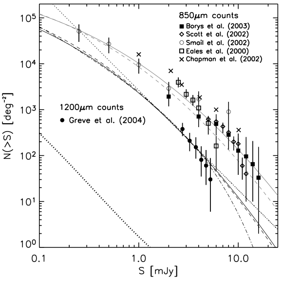
Figure 7: Cumulative number counts at $1200$$\mu$m (solid circles) based on the $\geq$$3.5\sigma$ MAMBO source catalogue presented in this paper. The error bars represent 95 per cent two-sided confidence levels on a Poissonian distribution. Also shown are $850$$\mu$m cumulative number counts from a number of recent SCUBA surveys. The dashed black and grey lines show the number counts at $1200$ and $850$$\mu$m , respectively, as predicted by a pure luminosity scenario in which $g(z)=(1+z)^{3}$ out to $z\rm=2$, beyond which no further evolution occurs. The solid black and grey curves represent predicted number counts at $1200$ and $850$$\,\mu$m, respectively, based on the galaxy evolution model by Jameson et al. (1999), see text for details. The thin dotted line corresponds to a simple power law with slope $\alpha=-2.2$, while the dark solid curve represents the Schechter function $dN/dS\propto(S/S_{o})^{-\alpha}exp(-S/S_{o})$, where $\alpha=2.3$ and $S_{o}=4$ mJy. Finally, the thick dotted line represent a no-evolution scenario.

In order to do so, we considered a simple parametric model which is based on the local $60$$\mu$m LF, $\Phi_{o}(L_{60})$, as derived from IRAS data (Saunders et al. 1990). The latter provides the best estimate of the far-IR LF of dusty galaxies in the local Universe to date, and is thus a useful template to try and model the number counts of dusty high-redshift galaxies. While a local $850$$\mu$m LF has been established by Dunne et al. (2000), who used SCUBA to observe a large number of galaxies from the IRAS Bright Galaxy Sample, the bright end of this function is still highly uncertain. Furthermore, if the majority of the MAMBO sources are at redshifts $z\rm>2$ and have similar dust temperatures to the IRAS galaxies (30–40 k), then the $60$$\mu$m LF will be a better approximation to the rest-frame far-IR LF of the MAMBO sources. We have therefore adopted the $60$$\mu$m LF as the reference LF at $z\rm=0$. In order to assess the evolution in the far-IR LF, we used a simple approach in which the LF at redshift $z$ is given by a simple scaling and/or translation of the local LF, i.e. $\Phi(L,z)=f(z)\Phi_{o}(L/g(z))$, where $f(z)$ and $g(z)$ are parametric models of the evolution in number density and luminosity, respectively. It is then straightforward to compute the cumulative source counts per unit solid angle brighter than a given flux density, $S_{\nu}$, as

$$N(\geq S_{\nu})=\int_{0}^{z_{max}}\int_{L_{min}(S_{\nu},z)}^{\infty}f(z)\Phi_{o}\left(\frac{L}{g(z)}\right)dlogL\frac{dV_{c}}{dz}dz,$$ (4)

where $dV_{C}/dz$ is the co-moving volume element per redshift increment, and $L_{min}(S_{\nu},z)=4\pi D^{2}_{L}S_{\nu}(1+z)^{-1}L_{\nu}/L_{\nu(1+z)}$ is the minimum luminosity observable for a source at redshift $z$ and a survey flux limit of $S_{\nu}$. The evolution functions $f(z)$ and $g(z)$ are constrained by the fact that their predictions of the extragalactic background, the observed number counts and redshift distribution has to be consistent with observations.

In Figure 7 we have plotted the predicted $1200$ and $850$$\mu$m number counts from a model with a luminosity evolution of $g(z)=(1+z)^{3}$ out to $z\rm=2$, beyond which the evolution is unchanged out to $z\rm=10$, which marks the high-redshift cut-off of the model. The model assumes the same SED for all sources — here we have adopted $T_{\rm d}=44$ k, $\beta=+1.2$, and a critical frequency of $\nu_{c}=2$ THz. While this pure-luminosity evolution model does an excellent job at reproducing the number counts at $1200$$\mu$m it fares less well at $850$$\,\mu$m, where it tends to slightly underpredict the number counts at bright flux levels.

Another parametric model is that of Jameson (1999) which employs a pure luminosity evolution of the form

$$g(z)=(1+z)^{3/2}sech^{2}\left(b\ln(1+z)-c\right)cosh^{2}c,$$ (5)

where $b=2.2\pm 0.1$ and $c=1.84\pm 0.1$, see also Smail et al. (2002). This model is arguably the most realistic of the parametric models, since it is motivated by semi-analytical models, i.e. models based on dark matter halo merging trees and assumptions about the astrophysics of the gas in halos. Furthermore, the model is not only in agreement with predictions of the chemical enrichment as a function of cosmic time but it also naturally includes a peak in the evolution at $z\rm\simeq 2$ which is in agreement with the recently determined redshift distribution of radio-identified SMGs (Chapman et al. 2003). In Figure 7 we have plotted the predicted $1200$ and $850$$\mu$m number counts for this model, under the assumption that the SEDs of all MAMBO and SCUBA sources are well matched by modified blackbody law with $T_{\rm d}=37$ k, $\beta=+1.5$, and a critical frequency of $\nu_{c}=2$ THz. It is seen that this physically more realistic model is able to reproduce both the MAMBO and SCUBA number counts extremely well, suggesting that the MAMBO and SCUBA sources trace the same population of high-redshift, far-IR-luminous, starburst galaxies.

While the mm number counts at faint as well as bright flux levels is still too poorly determined to warrant a detailed test of models of galaxy evolution, it is clear from the comparison with simple analytical model made above, that a scenario in which no evolution takes place at all, as illustrated by the thick dotted line in Figure 7, can be ruled out.

6 Clustering of MAMBO sources

The next big step forward in our understanding of SMGs is likely to come from determining how they are clustered. Their clustering properties may then provide a link to a present-day population of galaxies. If SMGs are the progenitors of massive elliptical galaxies, as suggested by their star-formation rates, molecular/dynamical masses and co-moving space densities, then they are expected to be strongly clustered. This follows from the way peaks in the density field in the early Universe are biased in mass (e.g. Benson et al. 2001). Giant ellipticals, being the most luminous objects in the local Universe, are often found residing in the centres of galaxy clusters; as such they pin-point the most overdense and therefore mass-biased regions in the Universe.

Submm surveys of various depths and sizes have searched for clustering among SMGs and have all failed to detect a significant signal (Scott et al. 2002; Webb et al. 2003; Borys et al. 2003). This has been due largely to the limited size of the survey regions, though efforts are further hampered by the fact the (sub)mm population spans a broad range in redshift — the quartile range is $z$ = 1.9–2.8 (Chapman et al. 2003, 2004) with a possible high-redshift tail extending to $z\rm\mathrel{\raise 1.50696pt\hbox{$\scriptstyle>$}\kern-6.00006pt\lower 1.72218pt\hbox{{$\scriptstyle\sim$}}}4$ — and any clustering signal will thus, when projected onto the sky, become heavily diluted. Any detection of angular clustering will therefore be a lower limit on the real 3D clustering. One lesson learned from these surveys was that very large ($\sim$1 square degree) areas containing several hundred sources with strong redshift constraints are required in order to determine the clustering properties of SMGs. Here, we present the results for the the MAMBO population using two independent clustering statistics.

The first test calculates the angular two-point correlation function, $w(\theta)$, which quantifies the excess probability of finding a source within an angle, $\theta$, of a randomly selected source, over that of a random distribution, i.e.

$$\delta P(\theta)=N^{2}(1+w(\theta))\delta\Omega_{1}\delta\Omega_{2},$$ (6)

where $\delta P(\theta)$ is the probability of finding a source within a solid angle $\delta\Omega_{1}$, and another source in another solid angle $\delta\Omega_{2}$ within a angular distance $\theta$ of each other (see e.g. Coles & Lucchin 2002). $N$ is the mean surface density of objects on the sky.

Several estimators of $w(\theta)$ have been suggested in the literature, and here we shall use the one first proposed by Landy & Szalay (1993):

$$w(\theta)=\frac{\langle DD\rangle-2\langle DR\rangle+\langle RR\rangle}{\langle RR\rangle},$$ (7)

where $\langle DD\rangle$ is the number of real source pairs which fall within a bin of width $\delta\theta$ in the map. $\langle RR\rangle$ is the number of random–random pairs extracted from simulated maps in which the sources are randomly distributed. Similarly, $\langle DR\rangle$ is the number of data–random pairs. In order to generate the random catalogues we created simulated maps by drawing sources from a source count model and placing them randomly throughout the field. We used the best fit to the observed number counts as provided by the Schechter function in section 5. Noise was added using one of the pure noise maps obtained by randomising the array parameters (section 4.2) thereby ensuring that the noise mimicked the properties of the real map as closely as possible. Mock source catalogues were then generated by applying our source extraction technique to the simulated maps. This exercise was repeated 500 times. By taking the ensemble average, the catalogues $\langle RR\rangle$ and $\langle DR\rangle$ were obtained. Furthermore, the $\langle RR\rangle$ and $\langle DR\rangle$ catalogues were normalised to have the same number of objects as $\langle DD\rangle$. The clustering analysis described here is similar to that of Borys et al. (2003) in the sense that our analysis takes the negative off-beams properly into account when estimating the clustering: our simulated maps have the same global chop-pattern as the real map. However, this effect is expected to be very small for MAMBO maps, where the off beams are smeared out due to sky rotation.

Figure 8: Angular two-point correlation function for ELAIS N2 (top) and the Lockman Hole (bottom). The two-point correlation function based on the $\geq$$3.0\sigma$ sample (empty squares) uses a bin size of $30\mbox{${}^{\prime\prime}$}$, while the correlation function based on the $\geq$$3.5\sigma$ catalogue (filled circles) is derived using a bin size of $35\mbox{${}^{\prime\prime}$}$. The solid line is the best-fit power-law correlation function found by Daddi et al. (2000) for EROs with $R-K>\rm 5$ and $K<\rm 18.5$. The dotted line represents the correlation function for LBGs as determined by Giavalisco & Dickinson (2001). The errors are given by $\delta w(\theta)=\left(\frac{1+w(\theta)}{\langle DD\rangle}\right)^{1/2}$.

The resulting two-point correlation functions obtained using the $\geq$$3.5\sigma$ as well as the $\geq$$3.0\sigma$ catalogues for the ELAIS N2 and Lockman Hole fields are shown in Figure 8. The bin sizes used were $\delta\theta=35\mbox{${}^{\prime\prime}$}$ and $30\mbox{${}^{\prime\prime}$}$, respectively, both of which roughly corresponds to two times the MAMBO beam and furthermore ensures an adequate number of sources in each bin. It is seen from Figure 8 that the two-point correlation function for the Lockman Hole is consistent with zero within the error bars at all angular scales. In the ELAIS N2 field, however, the correlation function has a gradient, showing a slight excess correlation at small angular scales and an anti-correlation at scales of $\sim 500\mbox{${}^{\prime\prime}$}$. The correlation functions based on the $\geq$$3.5\sigma$ and $\geq$$3.0\sigma$ catalogues both show this trend. The correlation seen at $\theta\mathrel{\raise 1.50696pt\hbox{$\scriptstyle<$}\kern-6.00006pt\lower 1.72218pt\hbox{{$\scriptstyle\sim$}}}100\mbox{${}^{\prime\prime}$}$ seems to be apparent by looking at the map, from which it appears that the sources are distributed in ’clusters’, one of which is located $\sim$200^′′ south-west of the map centre, and another $\sim$350^′′ south-east from centre. Within these clusters, the sources are typically separated by $\sim$20–80^′′, which could explain the excess correlation seen on these scales. The anti-correlation at $\theta\sim 500\mbox{${}^{\prime\prime}$}$ is reflected in the overall distribution of sources in the ELAIS N2 field which shows the sources to be distributed around a void slightly north-east of the map centre. A similar void, although less significant, is seen south-east of the centre of the Lockman Hole map. These voids appear to be real: not only are there no sources detected in these regions with SCUBA, but the $\mu$Jy radio population also seems to have a similar spatial distribution (Ivison et al. 2002). The good correspondence between these three populations suggests that the structure seen is real large-scale structure. A more detailed analysis of this will be presented in a future paper (Greve et al., in preparation).

An alternative test for clustering is the so-called nearest-neighbour analysis (Scott & Tout 1989). This considers the distribution of nearest neighbour separations, $\theta$, of sources on a sphere. For a random distribution of sources, the probability density function can be shown to be:

$$P(\theta)d\theta=\frac{N-1}{2^{N-1}}\sin\theta(1+\cos\theta)^{N-2}d\theta,$$ (8)

where $N$ is the number of objects in the sample — see Scott & Tout (1989) for details. We performed a nearest-neighbour analysis on the $\geq$$4.0\sigma$ source catalogues in each field, and the resulting nearest-neighbour distributions are shown as black lines in Figure 9. First of all, it is notable that the nearest-neighbour distributions for the two fields look remarkably similar. In particular, both distributions show a significant peak at angular scales of $\sim$23^′′. Changing the bin size to values in the range 11–17^′′ does not alter the overall appearance of the distributions significantly, and the over-density of sources in the 15–30^′′ bin remains. In order to compare the angular distribution of MAMBO sources with a random distribution, we used the same 500 $\langle RR\rangle$-catalogues which were used in connection with the two-point correlation function. The ensemble-averaged nearest-neighbour distributions for these simulated maps are shown as grey curves in Figure 9.

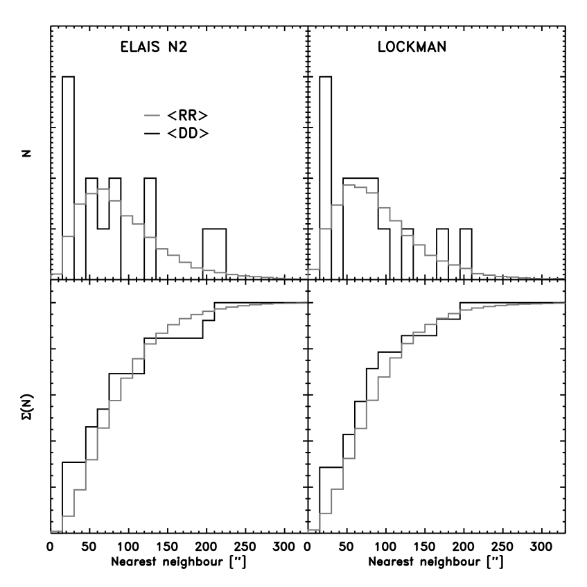
Figure 9: Distributions of nearest-neighbours in the ELAIS N2 (left column) and the Lockman Hole (right column). The black curves represent the actual data (the $\geq$$4.0\sigma$ source catalogues), while the red curves are the ensemble averaged distributions obtained from 500 simulated maps of the two fields.

It is seen that the random distributions do not peak at $\sim$15–30^′′ but at $\theta\simeq 60\mbox{${}^{\prime\prime}$}$ which is in accordance with the probability density function in eq. 8. From a Kolmogorov-Smirnoff (K–S) test we find that in both fields the probability of the $\langle DD\rangle$ and $\langle RR\rangle$ distributions being drawn from the same underlying distribution is about 10 per cent. In other words, there is a 10 per cent chance of a random distribution yielding a more paired distribution than that observed for the MAMBO sources. A similar analysis on the $\geq$$3.5\sigma$ sample shows a similar significant peak at $\sim$15–30^′′.

Thus, while we haven’t found a significant clustering signal from the two-point correlation function, there is tentative evidence from the nearest-neighbour analysis that MAMBO sources are not randomly distributed but tend to come in pairs. This is qualitatively in agreement with a recent study which utilises the results from the spectroscopic survey of radio-bright SMGs to search for pairs and/or triplets of sources in redshift space. This has yielded a significant detection of the clustering of SMGs and has constrained the correlation length to $r_{0}\simeq 6.1\pm 2.1$h^-1 Mpc (Blain et al. 2004; Smail et al. 2003).

7 Comparison with the SCUBA UK 8 mJy Survey

While a detailed analysis of the properties of the MAMBO sources at radio and optical/near-IR wavelengths shall be presented in Paper II (Greve et al., in preparation), it is appropriate here to compare the MAMBO and SCUBA maps. Such a comparison is meaningful since as we saw in section 5 both surveys reach very similar integral counts, and a ’typical’ $z\sim 2.5$ starburst SED will hit the flux limit in both surveys almost simultaneously.

7.1 The reliability of (sub)mm surveys

First of all, such a cross-check between the MAMBO and SCUBA catalogues will allow us to assess the reliability of (sub)mm surveys. As already mentioned, (sub)mm surveys in general have adopted detection thresholds at low signal-to-noise ratios (typically $3.0$–$3.5\sigma$ - see e.g. Eales et al. 2000; Scott et al. 2002; Webb et al. 2003; this work), and confusion has been a major issue for these surveys. In addition, different surveys have used different data-reduction software, and widely differing source extraction techniques have been adopted.

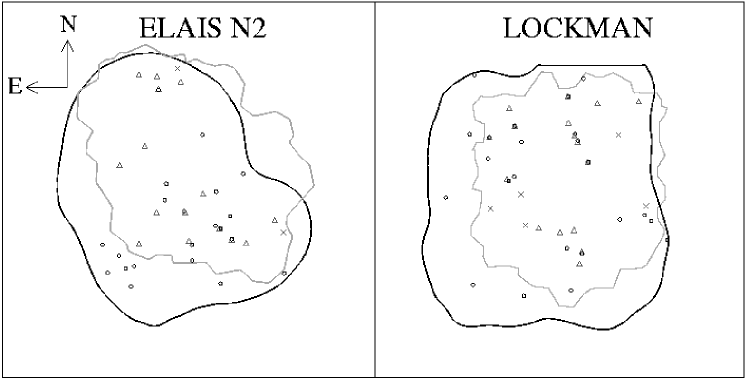
Figure 10: Distribution of MAMBO and SCUBA sources detected at $\geq$$3.5\sigma$ in the ELAIS N2 and Lockman Hole fields (this paper; Scott et al. 2002). The black circles are sources detected by MAMBO while grey triangles are SCUBA detections. The crosses denote the seven SCUBA sources which were deemed spurious and therefore rejected by Ivison et al. (2002) due to their lack of radio identifications and high associated noise levels. The MAMBO and SCUBA survey regions are outlined in black and grey, respectively, see also Figure 1. The boxes are $21\mbox{$\stackrel{{\scriptstyle\prime}}{{\textstyle.}}$}7\times 21\mbox{$\stackrel{{\scriptstyle\prime}}{{\textstyle.}}$}7$.

The comparison between the MAMBO and SCUBA $\geq$$3.5\sigma$ source catalogues is shown in Figure 10, which shows the outline of the MAMBO and SCUBA maps with the $\geq$$3.5\sigma$ $850$$\mu$m sample as given by Scott et al. (2002) and the $\geq$$3.5\sigma$ $1200$$\mu$m sources presented in this paper overplotted. It is seen immediately that four SCUBA sources in ELAIS N2 are unambiguously detected at $1200$$\,\mu$m, while in the Lockman Hole eight SCUBA sources have been confirmed with MAMBO.

It is interesting to see how these MAMBO identifications are distributed in terms of signal-to-noise and whether the identification rate increases if we lower the source detection threshold to $3.0\sigma$. In order to do so, we have compared the $4.0$, $3.5$, and $3.0\sigma$ SCUBA source lists of Scott et al. with our corresponding MAMBO source catalogues, and for each SCUBA source we computed the distance to the nearest MAMBO source. The resulting distributions are shown in Figure 11. For both fields the distribution is seen to peak at offsets smaller than 10^′′. In fact, both distributions seem to show that a cutoff in positional offset of $<10\mbox{${}^{\prime\prime}$}$ is a natural selection criterion as to whether a MAMBO source is a genuine counterpart to a SCUBA source or not. This is in line with what we would expect given the fwhms of the MAMBO and SCUBA beams. Adopting this criterion and using the $\geq$$3.0/3.5/4.0\sigma$ catalogues from both surveys, we confirm 6/4/3 out of 36/17/7 SCUBA sources in the ELAIS N2 field and 9/8/5 out of 36/21/12 SCUBA sources in the Lockman Hole, respectively. Thus, the identification rate clearly increases with signal-to-noise, from 17–25 per cent for the $3.0\sigma$-catalogues to 43 per cent in ELAIS N2 and 42 per cent in the Lockman Hole for the $4.0\sigma$-catalogues. At face value, our MAMBO survey thus confirms about half of the most significant SCUBA sources.

Figure 11: Distribution of offsets between SCUBA sources and their nearest MAMBO counterpart in the ELAIS N2 (top panel) and Lockman Hole fields (bottom panel). The $4.0$, $3.5$, and $3.0\sigma$ MAMBO samples are compared with the $4.0$, $3.5$, and $3.0\sigma$ SCUBA samples of Scott et al. (2002), and the corresponding distributions are shown as solid, dashed and dotted curves, respectively.

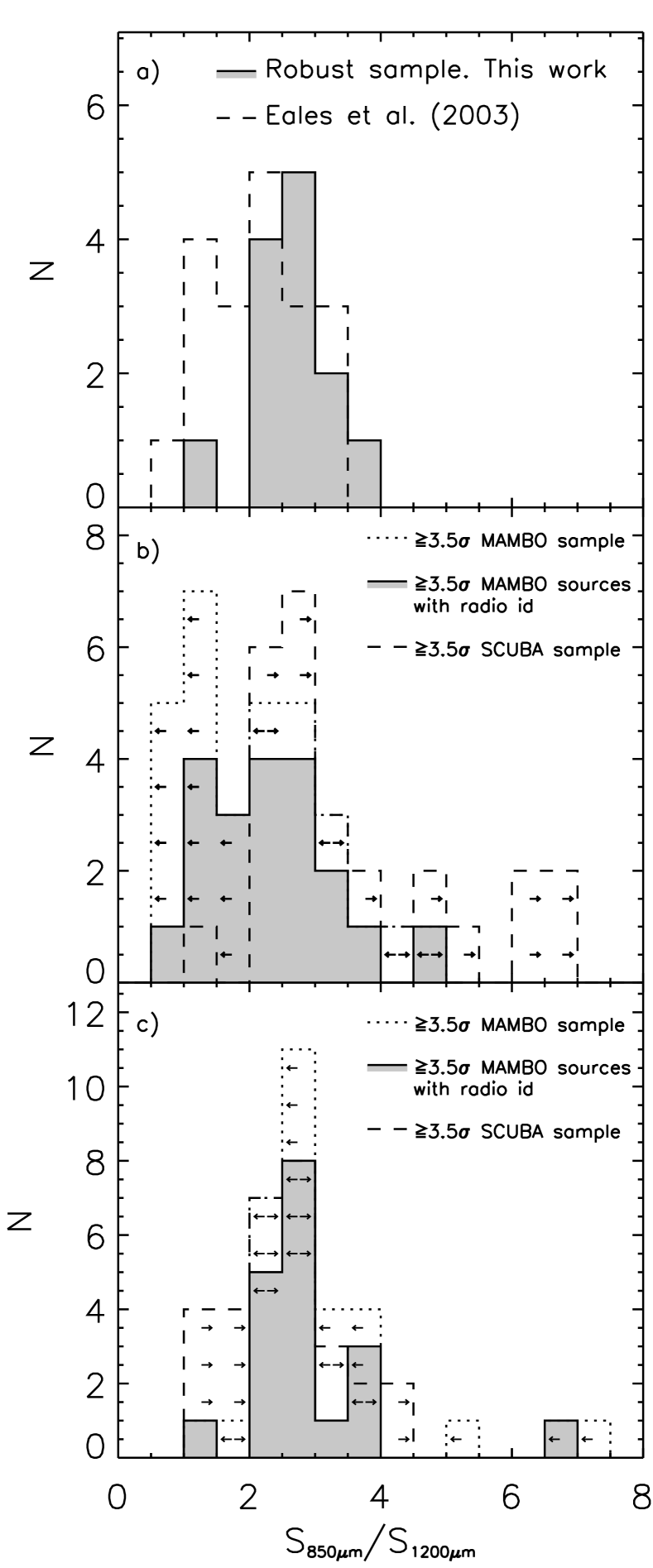
Figure 12: a) The distribution of $850/1200$$\mu$m flux ratios for the 13 $\geq$$3.5\sigma$ SCUBA sources identified with MAMBO in this paper (light-grey shaded area), and for the sample presented by Eales et al. (2003) (dashed line). b) The dotted histogram is the flux ratio distribution for all the $\geq 3.5\sigma$ MAMBO sources within the SCUBA regions, including the ones which were not detected by SCUBA. In the latter case upper flux limits were estimated as the peak flux within an aperture of radius 10^′′centered on the MAMBO position in the SCUBA map. The distribution of flux ratios for all the $\geq 3.5\sigma$ SCUBA sources (dashed histogram) were obtained in a similar manner by measuring the peak flux in the MAMBO map within a 10″radius of the SCUBA position. The light-grey shaded histogram represents the distribution for the subset of MAMBO sources which were robustly identified in the radio. c) The same as b) except more conservative upper flux limits ($2\sigma+F$) were adopted, see text for details.

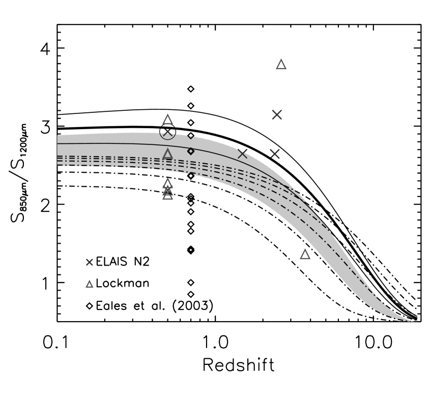
Figure 13: The $850/1200$$\mu$m flux density ratio for SCUBA sources detected by MAMBO in the ELAIS N2 (crosses) and Lockman Hole (triangles). Six of the sources have spectroscopic redshifts (see Chapman et al. 2003, 2004), while the remainder have been placed at $z\rm=0.5$. The two encircled sources have no radio counterpart. Shown as diamonds are the $850/1200$$\mu$m flux ratios for the sample of Eales et al. (2003). The thick solid curve represents the expected flux ratio for an optically thin modified blackbody with $T_{\rm d}=45$ K and $\beta=+1.5$, typical for a local ULIRG. This curve is enveloped by two thin solid curves which correspond to changes in the dust temperature and spectral index of $\Delta T_{\rm d}=\pm 5$ K and $\Delta\beta=\pm 0.2$. The light-grey shaded area corresponds to a modified blackbody with $T_{\rm d}=(35.6\pm 5.0)$ K and $\beta=(+1.3\pm 0.2)$. The dot-dashed curves corresponds to SEDs with $\beta=1.0$ and $T_{d}=20...70$ K in step if 10 K.

An additional 24 hr of $850$$\mu$m data — not used in the original 8 mJy Survey — resulted in a slightly different source catalogue than that given in Scott et al. (2002). With the inclusion of the new data, the significance of N2 850.17 drops from $3.5\sigma$ to $3.3\sigma$, with a new flux density of $5.3\pm 1.7$ mJy, while N2 850.16 disappears (see Ivison et al. 2002). At the position of N2 850.17 in the MAMBO map, we detect a source at the $2.7\sigma$ significance level, suggesting that N2 850.17 is a real source, even though it is just below the formal $3.5\sigma$ detection threshold of the 8 mJy Survey. N2 850.16, however, is not detected at $1200$$\mu$m at greater than $1\sigma$ significance, confirming that this was a spurious source in the original Scott et al. map.

Based on extremely deep radio imaging of the 8 mJy fields, Ivison et al. (2002) concluded that six of the original SCUBA sources in the ELAIS N2 and Lockman Hole fields were likely to be fake sources. Not only were they extracted from extremely noisy regions, but they also lacked a radio counterpart despite being amongst the brightest SMGs in the sample. The sources in question were LE 850.9, LE 850.10, LE 850.11, LE 850.15, LE 850.20, and N2 850.14. From Figure 10 it is seen that none of these sources, which are denoted by grey crosses, coincide with a $\geq$$3.5\sigma$ MAMBO source. In fact, the highest significance 1200$\mu$m detection of the above sources was at the 1.6-$\sigma$ level. Hence, our MAMBO maps strengthen the conclusion of Ivison et al. (2002) that these sources are spurious. If we compare the MAMBO catalogue with the refined SCUBA source catalogue, in which the above mentioned SCUBA sources (including N2 850.16 and N2 850.17) have been omitted, we find that at the $\geq$$3.0/3.5/4.0\sigma$ level, we confirm 6/4/3 out of 33/14/7 SCUBA sources in the ELAIS N2 field and 9/8/5 out of 31/16/9 SCUBA sources in the Lockman Hole, respectively. Hence, the MAMBO identification rate of SCUBA sources in the Lockman Hole increases to 56 per cent, which is becoming comparable to fraction of SMGs detected in deep radio maps (Smail et al. 2000; Ivison et al. 2002).

An important point to make in this context is that Figure 10 clearly shows that while not all SCUBA sources are detected by MAMBO, there is a good overall spatial correspondence between SCUBA and MAMBO sources, as was also pointed out in section 6. One way to interpret this result is that the two surveys represent two different realisations of the same large-scale structure. From two independent but similar (sub)mm surveys of the same region, we would expect to find the most significant sources in both surveys, but this is not necessarily true of the fainter sources near the detection threshold.

Table 4: MAMBO and VLA radio identifications of the SCUBA 8 mJy Survey $\geq$$3.5\sigma$ source catalogue (Scott et al. 2002). The $850$$\mu$m and 1.4 GHz radio flux densities are from Scott et al. (2002) and Ivison et al. (2002), respectively.

SCUBA ID	$S_{850\mu\rm{m}}\pm\sigma_{850\mu\rm{m}}$	MAMBO ID	$S_{1200\mu\rm{m}}\pm\sigma_{1200\mu\rm{m}}$	SCUBA/MAMBO Offset	RADIO	$S_{1.4\rm{GHz}}\pm\sigma_{1.4\rm{GHz}}$
	mJy		mJy	′′		$\mu$Jy
$\sigma\geq 4.0$ Detections
N2 850.1	$11.2\pm 1.6$				yes	$45\pm 16$
N2 850.2	$10.7\pm 2.0$	N2 1200.39	$3.4\pm 1.1$	8.4	yes	$92\pm 16$
N2 850.3	$8.5\pm 1.6$	N2 1200.19	$2.9\pm 0.8$	5.1	no	$<44$
N2 850.4	$8.2\pm 1.7$	N2 1200.10	$3.1\pm 0.7$	4.5	yes	$221\pm 17$
N2 850.5	$8.5\pm 2.2$	N2 1200.3	$3.9\pm 0.8$	1.0	yes	$77\pm 31$
N2 850.6	$9.2\pm 2.4$				no	$38\pm 19$
N2 850.7	$9.0\pm 2.4$	N2 1200.4	$3.4\pm 0.7$	4.0	yes	$159\pm 27$
$4.0>\sigma\geq 3.5$ Detections
N2 850.8	$5.1\pm 1.4$				yes	$74\pm 29$
N2 850.9	$9.0\pm 2.5$				yes	$33\pm 12$
N2 850.10	$5.4\pm 1.5$				no	$58\pm 24$
N2 850.11	$7.1\pm 2.0$				no	$<44$
N2 850.12	$5.5\pm 1.6$				no	$32\pm 17$
N2 850.13‡	$6.3\pm 1.9$				yes	$99\pm 23$
N2 850.14∗	$11.2\pm 3.3$				no	$<44$
N2 850.15	$5.0\pm 1.5$				no	$31\pm 20$
N2 850.16†	$12.9\pm 3.9$				no	$<44$
N2 850.17††	$5.3\pm 1.7$				no	$<44$
$\sigma\geq 4.0$ Detections
LE 850.1	$10.5\pm 1.6$	LE 1200.5	$3.4\pm 0.6$	5.1	yes	$73\pm 10$
LE 850.2	$10.9\pm 2.4$	LE 1200.1	$4.8\pm 0.6$	1.3	yes	$29\pm 11$
LE 850.3	$7.7\pm 1.7$	LE 1200.11	$2.9\pm 0.7$	6.2	yes	$98\pm 12$
LE 850.4	$8.3\pm 1.8$				no	$19\pm 8$
LE 850.5	$8.6\pm 2.0$				no	$<25$
LE 850.6	$11.0\pm 2.6$	LE 1200.10	$2.9\pm 0.7$	7.7	yes	$54\pm 14$
LE 850.7	$8.1\pm 1.9$				yes	$135\pm 13$
LE 850.8	$5.1\pm 1.3$	LE 1200.14	$2.4\pm 0.6$	3.9	yes	$58\pm 12$
LE 850.9∗	$12.6\pm 3.2$				no	$<23$
LE 850.10∗	$12.2\pm 3.1$				no	$<25$
LE 850.11∗	$13.5\pm 3.5$				no	$26\pm 12$
LE 850.12	$6.2\pm 1.6$				yes	$278\pm 12$
$4.0>\sigma\geq 3.5$ Detections
LE 850.13	$9.8\pm 2.8$				no	$18\pm 11$
LE 850.14	$9.5\pm 2.8$	LE 1200.3	$3.6\pm 0.6$	2.0	yes	$72\pm 12$
LE 850.15∗	$11.7\pm 3.4$				no	$<21$
LE 850.16	$6.1\pm 1.8$	LE 1200.6	$2.8\pm 0.5$	2.6	yes	$41\pm 12$
LE 850.17	$9.2\pm 2.7$				no	$<23$
LE 850.18	$4.5\pm 1.3$	LE 1200.12	$3.3\pm 0.8$	3.1	yes	$47\pm 10$
LE 850.19	$5.5\pm 1.6$				no	$<27$
LE 850.20∗	$10.3\pm 3.1$				no	$<24$
LE 850.21	$4.5\pm 1.3$				yes	$21\pm 10$
‡ Detected with MAMBO at the $2.8\sigma$ level.
∗ Excluded from the refined 8 mJy sample of Ivison et al. (2002).
† This source vanished with the inclusion of an additional 24 hr of SCUBA data.
†† This source dropped from $3.5$ to $3.3\sigma$ with the inclusion of additional SCUBA data. It is detected with MAMBO at $2.7\sigma$.

Deep radio observations provide an alternative route to reliably identify SMGs. About two thirds of SMGs are detected in the radio where the ratio of submm to radio flux detection thresholds is above $\sim$400 (Smail et al. 2000; Ivison et al. 2002). However, it remains an open question whether the third of the population which are radio-blank are SMGs at very high redshifts ($z>>3$), or cooler, less-far-IR-luminous objects at similar redshifts as the bulk of the population, or simply spurious sources. All three scenarios would explain the lack of radio counterparts.

In Table LABEL:table:scubo-list we list all the $\geq$$3.5\sigma$ SCUBA sources with a MAMBO counterpart detected at $\geq$$3.0\sigma$ significance within 10^′′, along with their positional offsets and flux densities at $1200$ and $850$$\,\mu$m. Of the 12 $\geq$$3.5\sigma$ SCUBA sources in the ELAIS N2 field which were not detected by MAMBO, only four had a radio identification. Of the eight radio-blank SCUBA sources, only one — N2 850.3 — was confirmed by MAMBO, indicating that it could be cool, or lie at $z>>3$. In the Lockman Hole, none of the radio-blank SCUBA sources were detected at $1200$$\,\mu$m, and only three of the 11 radio-identified SCUBA sources were not detected by MAMBO.

Since the depth of the MAMBO maps at $1200$$\mu$m is comparable to that of the SCUBA maps at $850$$\mu$m it is hard to conceive of a way in which an $850$$\mu$m source with no radio counterpart could fail to be detected at $1200$$\mu$m . The only plausible explanations require that the sources are spurious or confused.

In Table 5 we have summarised the above findings. They suggest strongly that the fraction of robust SCUBA sources, i.e. sources confirmed by MAMBO, which are not detected in the radio is low: 20 per cent (1/5) in ELAIS N2 and 0 per cent in the Lockman Hole. These findings suffer from small number statistics and we await a comparison between the much larger map of the Lockman Hole being obtained with MAMBO (Bertoldi et al. in prep.) and the SCUBA map of that region which is being obtained as part of SHADES (see http://www.roe.ac.uk/ifa/shades/).

In the light of current and future (sub)mm surveys, our findings underline the importance of multi-wavelength follow-up in order to establish the reality of (sub)mm sources, and the dependence only on the most robust samples to draw meaningful statistical conclusions (cf. Dannerbauer et al. 2004).

Table 5: The number (and percentage) of SCUBA sources identified by MAMBO divided into radio and non-radio ID categories. Note, that all the number in this table are based on the comparison with the $\geq$$3.5\sigma$ 8 mJy Sample of Scott et al. (2002) and the $\geq$$3.0\sigma$ MAMBO sample presented in this paper.

	MAMBO ID			No MAMBO ID
Field
	Radio ID	No Radio ID	Total	Radio ID	No Radio ID	Total
ELAIS N2	4	1	5	4	8	12
Lockman	8	0	8	3	10	13
Total	12 (92%)	1 (8%)	13	7 (28%)	18 (72%)	25

7.2 The $850/1200$$\mu$m flux density ratio

Another valuable piece of information which can be gleaned from a comparison of the MAMBO and SCUBA maps is the $850/1200$$\mu$m flux ratios for a large sample of (sub)mm galaxies. Beyond $z\geq\rm 3$ this flux ratio becomes a strong function of redshift, and can thus be used as a crude discriminator between low- and high-redshift sources (Eales et al. 2003), much in the same way that the radio-to-submm spectral index acts as a redshift estimator for sources at $z\mathrel{\raise 1.50696pt\hbox{$\scriptstyle<$}\kern-6.00006pt\lower 1.72218pt\hbox{{$\scriptstyle\sim$}}}\rm 3$ (Carilli & Yun 1999, 2000). Thus, the two redshift estimators complement each other, and if used in combination can potentially be used to probe the redshift distribution of (sub)mm sources. However, both of these redshift estimators suffer from the $T_{\rm d}-z$ degeneracy first pointed out by Blain (1999), which implies that a low-redshift source with a cold dust temperature is indistinguishable from a warm source at high redshift.

The distribution of $850/1200$$\mu$m flux ratios for the 13 $\geq$$3.5\sigma$ SCUBA sources which were robustly identified by our MAMBO survey are plotted in Figure 12a, along with the ratios for a sample of SCUBA-observed MAMBO sources by Eales et al. (2003). Using SCUBA in its photometry mode, they observed 21 MAMBO-selected sources from the MAMBO Deep Field Survey (Bertoldi et al., in preparation). While there is a considerable overlap between the two distributions, the latter has a significant over-density at low values which is not reproduced by our sample. From our sample we find a median value of $S_{850}/S_{1200}=2.6\pm 0.6$, marginally higher than the median value of $2.1\pm 0.7$ found by Eales et al. (2003), although within the scatter.

In Figure 13 we have plotted the measured $850/1200$$\mu$m flux ratios of our sample and the Eales et al. sample along with curves showing the predicted $850/1200$$\mu$m flux density ratios against redshift for an SED with $T_{\rm d}=45$ K and $\beta=+1.5$, and an SED with $T_{\rm d}=35.6$ K and $\beta=+1.3$. The former SED provides a good match to the local ULIRG, Arp 220, while the latter is based on the average $T_{\rm d}$ and $\beta$ values derived from the SCUBA Local Universe Galaxy Survey (Dunne et al. 2000). In addition, we have also plotted the $S_{850\mu\rm{m}}/S_{1200\mu\rm{m}}$–$z$ relationship for a set of SEDs with $\beta=1$ and $T_{d}=20,30...70$ K, i.e. SEDs which have very different dust properties from local ULIRGs. Note, the above dust temperatures are at a redshift of zero. In order to account for the increasing cosmic microwave background radiation (CMBR) temperature with redshift and its thermal coupling with the dust we have used

$$T_{d}(z)=\left(T_{d,z=0}^{4+\beta}+T_{\rm CMBR}^{4+\beta}\left[(1+z)^{4+\beta}-1\right]\right)^{1/(4+\beta)},$$ (9)

where $T_{\rm CMBR}$ is the present epoch CMBR temperature, (see e.g. Eales & Edmunds 1996). The effect is only significant when the dust is cold relative to the CMBR temperature, and therefore becomes more important at very high redshifts. The slight downward trend in the $S_{850\mu\rm{m}}/S_{1200\mu\rm{m}}$ curves at low redshifts is due to the negative spectral slope ($\alpha=-0.7$) of the radio continuum emission which boosts the $1200$$\mu$m flux relative to the flux at $850$$\mu$m . However, this effect is completely negligible at redshifts beyond $z\sim\rm 0.5$.

The low flux ratios found by Eales et al. (2003) led them to conclude that a significant fraction of SMGs must lie at very high redshifts ($z\rm>>3$) or possess dust properties different from low-redshift starburst galaxies. In contrast, we find no conflict between our measured $S_{850\mu\rm{m}}/S_{1200\mu\rm{m}}$ ratios and SEDs based on local ULIRGs. From a subset of five sources which have been targeted spectroscopically by Chapman et al. (2003, 2004), and thus are placed at their correct redshift in Figure 13, we can conclude that the observed flux ratios for at least four of the five sources are consistent with the range of SEDs expected from local ULIRGs. The one exception is the outlying point at $S_{850\mu\rm{m}}/S_{1200\mu\rm{m}}=\rm 3.8$ This data point corresponds to the source LE 850.6/LE 1200.10 which has another source (LE 1200.9) close to it. This source was detected by MAMBO but not by SCUBA, and it is likely that LE 1200.9 contributes to the 850$\mu$m flux of LE 850.6, leading to an artificially high flux ratio for this source.

Our sample is taken from two unbiased surveys at slightly different (sub)mm wavelengths and is thus independent of any radio selection bias. Furthermore, it is clear from Figure 13 that the SMG without a radio counterpart (circled symbol) does not have a lower $850/1200$$\mu$m flux ratio than the rest of the sample. This suggest that the source is blank in the radio because it is a cooler, less-far-IR-luminous object at similar redshifts to the bulk of the population, not because it lies at a very high redshift.

Candidates for very-high-redshift sources, i.e. 850$\mu$m dropouts, should be sought amongst sources detected by MAMBO but not SCUBA. From Figure 10 it is seen that 9 MAMBO sources in the ELAIS N2 field and 9 in the Lockman Hole fall within the regions observed by SCUBA, yet are not detected at $\geq$$3.5\sigma$ significance at $850$$\,\mu$m. Upper limits on the flux densities at $850$$\mu$m of these sources were measured, taking the peak flux in a 10″radius aperture region of the SCUBA map coincident with the MAMBO position. These limits were then merged with the $850$$\mu$m fluxes of the robust sample, resulting in $850$$\mu$m flux estimates (or upper limits) for all the 9+9+13=31 MAMBO sources which lie within the SCUBA regions. The resulting distribution of $850$-to-$1200$$\mu$m flux ratios is shown as the dotted curve in Figure 12b. The distribution appears to have two peaks, one at $S_{850\mu\rm{m}}/S_{1200\mu\rm{m}}\sim 1$ which reproduces the low-end tail of Eales et al. (2003) rather well and is almost entirely due to the MAMBO sources not detected by SCUBA, and another at $\sim 2.5$ which stems from the 13 sources robustly identified at both 1200$\mu$m and 850$\,\mu$m.

In order to make a fair comparison with the flux ratios of the SCUBA sample, we estimated 1200$\mu$m fluxes for all the SCUBA sources. This was done in an identical fashion as above, i.e. upper 1200$\mu$m flux limits were derived for the SCUBA sources not detected with MAMBO using the peak flux within a 10^′′radius aperture region of the MAMBO map centered on the SCUBA position, and concatenated with the robust sample. This distribution is shown as the dashed histogram in 12b.

The dotted and dashed distributions appear to be distinct, and in order to determine the probability of the two samples being drawn from the same parent distribution, we have employed the standard ’survival analysis’ tests (Feigelson & Nelson 1985), which are appropriate in the case where the samples contain upper or lower limits (censored data). This included the Gehan, log rank, Peto-Peto, and Peto-Prentice tests, the latter being perhaps the most conservative and least sensitive to differences in the censoring patterns. However, common to all the tests is that they are unable to compare samples with mixed censor indicators, i.e. one cannot compare a sample containing upper limits with a sample containing lower limits. As a result we ran the tests where only one of the samples contained censored data, assuming that the limits in the other sample were not limits but measured values, and vice versa. In both cases the tests yielded probabilities less than 0.01, thereby strongly suggesting that the two distributions are significantly different. This argues in favour of there being a low-end tail consisting of galaxies at either high redshifts or with cool dust temperatures. Consistent with these findings is the distribution of MAMBO sources with radio counterparts (shaded histogram in Figure 12b) which shows that few of the sources with flux ratios $\mathrel{\raise 1.50696pt\hbox{$\scriptstyle<$}\kern-6.00006pt\lower 1.72218pt\hbox{{$\scriptstyle\sim$}}}1.5$ are identified in the radio. This is what one would expect if they were at high redshifts or cool, not very far-IR luminous systems.

In addition to the two astrophysical explanations (i.e. cold dust or high redshift) Eales et al. also suggest more mundane reasons for their low flux ratios, the most important of which is astrometric errors (see discussion in Eales et al. 2003). For all but five of their 21 sources, they used positions derived from radio observations or mm-wave interferometry. For the remaining sources they used the MAMBO positions. With our dataset, in conjunction with the 8 mJy Survey images, we can reproduce the Eales et al. experiment in the case where only MAMBO positions are available. In order to do this we consider the sample of 13 sources which were detected by both MAMBO and SCUBA. However, instead of using the 850$\mu$m fluxes reported by Scott et al. (2002), we measure the 850$\mu$m flux at the MAMBO position in the SCUBA map using the peak flux within a 10^′′aperture. In general, we find that the effects of positional errors are small, and the flux ratios are not skewed towards lower values.

Finally, it is possible that contamination by spurious or flux-boosted MAMBO sources is responsible for at least some of the low flux ratios observed. However, based the Monte Carlo simulations in section 4.2 we expect no more than 2 sources to be spurious in each of the MAMBO maps. This is an upper limit, given that the overlap between the SCUBA and MAMBO regions is only about 68 per cent of the areas covered by MAMBO.

While the above analysis suggests that astrometrical errors and spurious/flux-boosted sources are unable to account for the 12 MAMBO sources with $S_{850\mu\rm{m}}/S_{1200\mu\rm{m}}\mathrel{\raise 1.50696pt\hbox{$\scriptstyle<$}\kern-6.00006pt\lower 1.72218pt\hbox{{$\scriptstyle\sim$}}}\rm 1.5$, we caution that the low flux ratio could be due to the way we have estimated the upper flux limits. Simply adopting the peak flux within a 10″aperture might in some cases result in too low flux estimates and would tend to bias the MAMBO and SCUBA distributions towards lower and higher flux ratios, respectively. In Figure 12c we have adopted a more conservative approach in which the upper limits on the fluxes were estimated by adding $2\times\sigma$ to the peak flux, where $\sigma$ is the local rms noise. Clearly, the overlap between the two distributions is now much greater, and the two distributions appear to be indistinguishable. This is confirmed by the ’survival analysis’ tests which yield probabilities in the range 0.22 (log rank) to 0.11 (Peto-Prentice) and similar for the reverse comparison, i.e. comparing the SCUBA distribution with the uncensored MAMBO distribution. Thus, adopting what is arguably more realistic upper flux limits we find no evidence for SMGs with unusually low 850-to-1200$\mu$m flux ratios as reported by Eales et al. (2003). If this is the case, the major implication is that, beyond the few completely unrepresentative submm-loud AGN at $z>4$, there is no significant population of SMGs at very high redshifts. The redshift distribution of radio-identified SCUBA sources, as determined by Chapman et al. (2003, 2004), would be applicable to virtually all of the (sub)mm population.

However, while we find no conclusive evidence for ’850$\mu$m -dropouts’ a handful of MAMBO sources do seem to be good candidates for SMGs at $z>>5$. In particular, LE 1200.2 is one of the brightest sources in our survey, yet it is not detected by SCUBA nor is it seen in the radio. Pointed SCUBA photometry observations of this source would provide an accurate accurate estimate of its 850$\mu$m flux and confirm or dismiss its status as a ’850$\mu$m -dropout’.

Furthermore, with the completion of the MAMBO Deep Field Survey and the SCUBA Half Degree Extragalactic Survey, which will not only provide us with much larger samples but also a multitude of observations at complementary wavelengths, we should be able to obtain a much better census of the high-redshift tail of (sub)mm sources.

8 Conclusions

In this paper we have presented results from a MAMBO $1200$$\mu$m blank-field survey of the ELAIS N2 and Lockman Hole fields, covering a total of 357 arcmin² to a rms level of $\sim$0.8 mJy beam^-1. We detect 27 sources at $\geq$$4.0\sigma$ significance, and more than 40 sources at $\geq$$3.5\sigma$.

From the $\geq$$3.5\sigma$ catalogue we have derived accurate number counts over the flux range 3–5.5 mJy, and find evidence for a break at $S_{1200\mu\rm{m}}\rm\simeq 4$ mJy. This corresponds to a far-IR luminosity of $\sim 10^{13}\,\mbox{L${}_{\odot}\,$}$ for a modified blackbody with $T_{\rm d}=40$ K and $\beta=+1.5$ at $z\rm=2.5$. The observed $1200$$\mu$m source counts can be successfully reproduced by a simple parametric model for the evolution the local ULIRG population. Furthermore, this model also fits the $850$$\mu$m source counts which suggests that the MAMBO and SCUBA sources are drawn from the same population of dust-enshrouded starburst at high redshift.

Two independent tests were carried out with the aim of detecting clustering in the MAMBO population. Although, the angular two-point correlation function showed no evidence of clustering, a nearest neighbour analysis suggests that the most significant MAMBO sources are not randomly distributed but come in pairs, typically separated by 23^′′. Furthermore, the spatial distribution of sources appears to be non-random, with sources tending to reside in clusters surrounding large voids. The reality of these structures is strengthened by the good overall spatial correlation between the SCUBA, MAMBO and $\mu$Jy-level radio sources. This suggests that co-spatial surveys at the two slightly different (sub)mm wavelengths skim the brightest members of a numerous but faint population, yielding two similar but low-signal-to-noise visualisations of the true (sub)mm sky.

Our MAMBO survey confirms roughly half of the refined $\geq$$3.5\sigma$ SCUBA 8 mJy Survey sample (Scott et al. 2002; Ivison et al. 2002). This is comparable to the radio identification rate of SCUBA and MAMBO sources. As a by-product of this analysis, we have produced a extremely robust sub-sample of 13 SMGs detected at $\geq$$3.5\sigma$ by both SCUBA and MAMBO. We find that only one ($\sim$8 per cent) has no radio counterpart, a significantly lower fraction than the third which the radio-blank SMGs have generally been believed to constitute. Our results thus suggest that the population of SMGs which are detected by both SCUBA and MAMBO has no significant tail at $z\rm>>3$. This conclusion is further strengthened by the observed distribution of $850/1200$$\mu$m flux density ratios for the 13 sources in our sample. We find their flux density ratios to be consistent with the SEDs found for local ULIRGs and in agreement with the spectroscopic redshift distribution of SMGs as determined by Chapman et al. (2003, 2004).

Finally, we have identified 18 MAMBO sources within the SCUBA UK 8 -mJy regions which are not detected at $850$$\mu$m at greater than $3.0\sigma$ significance. Any high-redshift SMGs should be sought amongst this population of ’850$\mu$m -dropouts’. However, using conservative upper flux limits we find that the distribution of $850$-to-$1200$$\mu$m flux ratios for these sources is statistically indistinguishable from that of the sources identified robustly in both wavelengths.

References

- Barger et al. (1999) Barger, A.J., Cowie, L.L., & Sanders, D.B. 1999, ApJ, 518, 5L.
- Benson et al. (2001) Benson, A.J., Frenk, C.S., Baugh, C.M., Cole, S., & Lacey, C.G. 2001, MNRAS, 327, 1041.
- Bertoldi et al. (2000) Bertoldi, F., Menten, K.M., Kreysa, E., Carilli, C.L., & Owen, F. 2000, 24th meeting of the IAU, Joint Discussion 9, Manchester, England.
- Blain & Longair. (1993) Blain, A.W. & Longair, M.S. 1993, MNRAS, 265, L21.
- Blain (1999) Blain, A.W. 1999, MNRAS, 309, 955.