GRS 1915$+$105: The first three months with INTEGRAL

Abstract

GRS 1915$+$105 is being observed as part of an Open Time monitoring program with INTEGRAL. Three out of six observations from the monitoring program are presented here, in addition to data obtained through an exchange with other observers. We also present simultaneous RXTE observations of GRS 1915$+$105. During INTEGRAL Revolution 48 (2003 March 6) the source was observed to be in a highly variable state, characterized by 5-minute quasi-periodic oscillations. During these oscillations, the rise is faster than the decline, and is harder. This particular type of variability has never been observed before. During subsequent INTEGRAL revolutions (2003 March–May), the source was in a steady or “plateau” state (also known as class $\chi$ according to Belloni et al. 2000). Here we discuss both the temporal and spectral characteristics of the source during the first three months of observations. The source was clearly detected with all three gamma-ray and X-ray instruments onboard INTEGRAL.

1 Introduction

GRS 1915$+$105 has been extensively observed at all wavelengths ever since its discovery. It was originally detected as a hard X-ray source with the WATCH all-sky monitor on the GRANAT satellite (Castro-Tirado, Brandt & Lund 1992) with a flux of 0.35 Crab in the 6–15 keV range (Castro-Tirado et al. 1994). Subsequent monitoring with BATSE on CGRO showed it to be the most luminous hard X-ray source in the Galaxy (Paciesas et al. 1996), with L${}_{\rm 20-100keV}\sim 3-6\times 10^{38}$ erg s^-1 (for a distance of 12.5 kpc). Apparent superluminal ejections have been observed from GRS 1915$+$105 on at least two occasions: the first time in 1994 with the VLA (Mirabel & Rodríguez 1994) and the second time in 1997 with MERLIN (Fender et al. 1999). Both times the true ejection velocity was calculated to be $>0.9c$. Following the ejections of 1997, Fender et al. (1999) gave an upper limit for the distance to the source of 11.2$\pm$0.8 kpc. Recently, Chapuis & Corbel (2004) refined the distance to GRS 1915$+$105 to be 9.0$\pm$3.0 kpc. High optical absorption ($\geq 33$ magnitudes) towards GRS 1915$+$105 prevented the identification of the non-degenerate companion until recently. However, using the VLT, Greiner et al. (2001) identified the mass-donating star to be of spectral type K-M III. The mass of the black hole was deduced by Harlaftis & Greiner (2004) to be $14\pm 4.4\,{\rm M}_{\odot}$. The Rossi X-ray Timing Explorer (RXTE) has observed GRS 1915$+$105 since its launch in late 1995 and has shown the source to be highly variable on all timescales from milliseconds to months (see e.g. Belloni et al. 2000; Morgan, Remillard & Greiner 1997). Belloni et al. (2000) categorized the variability into twelve distinct classes. The source was detected up to $\sim$ 700 keV during OSSE observations (Zdziarski et al. 2001).

GRS 1915$+$105 is being observed extensively with the European Space Agency’s International Gamma-Ray Astrophysical Laboratory (INTEGRAL, Winkler et al. 2003) as part of the Core Program and also within the framework of an Open Time monitoring campaign. We also have a simultaneous observing campaign with RXTE to concentrate on timing analysis – these data are presented in Rodriguez et al. (2004a, b). First results from Revolution 48 were described in detail elsewhere (Hannikainen et al. 2003). During Revolution 48, the source was found to exhibit a new type of variability. Here we summarize the results from Revolution 48 and we present the results from two other observations which took place between 2003 April and May. In addition to our dedicated observations, GRS 1915$+$105 was in the field-of-view of INTEGRAL observations of Aql X-1 (Molkov et al. 2003) and SS 433 (Cherepaschuk et al. 2003). We exchanged data with both the PIs of the latter observations.

Table 1: Log of the INTEGRAL observations of GRS 1915$+$105. Data from Revolutions 49, 51, 53, 56, 58, and 60 were obtained from Molkov et al. (2003). Data from Revolution 70 obtained from Cherepaschuk et al. (2003).

Revolution #	Date	Exposure time
	(2003)	(ksec)
48	March 6	100
49	March 10	55
51	March 17	55
53	March 23	55
56	March 30	55
58	April 6	55
59	April 9	100
60	April 12	55
69	May 9	100
70	May 12	100

2 Observations

2.1 INTEGRAL and RXTE

As part of a monitoring program which consists of six 100 ks observations separated by approximately one month, INTEGRAL observed GRS 1915$+$105 for the first time for this campaign on 2003 Mar 6. Our campaign also included simultaneous coverage with the Rossi X-ray Timing Experiment (RXTE) – these data are discussed in Rodriguez et al. (2004a, 2004b). Two other observations were conducted in April and May 2003, and a further two in November (these latter will be discussed in a forthcoming paper). Table 1 shows the log of the Open Time observations of GRS 1915$+$105 – these include three from the monitoring program plus several obtained from the data exchange with other observers. Figure 1 shows the RXTE/ASM 2–10 keV lightcurve, and the shaded area indicates the dates from 2003 March 6 to May 12.

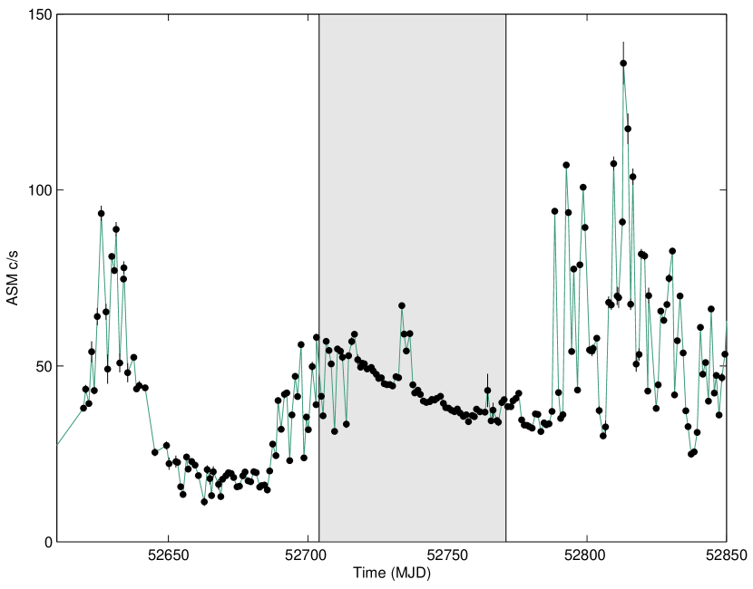
Figure 1: The RXTE/ASM 1-day average 2–10 keV lightcurve. The shaded area indicates the dates from 2003 Mar 6 (Rev48) to May 12 (Rev70).

The INTEGRAL observations were undertaken using the hexagonal dither pattern (Courvoisier et al. 2003) for Revolutions 48, 59 and 69: this consists of a hexagonal pattern around the nominal target location (1 source on-axis pointing, 6 off-source pointings, each 2 degrees apart and each science window of 2200 s duration). This means that GRS 1915$+$105 was always in the field-of-view of all three X-ray (JEM X-2) and gamma-ray (IBIS and SPI) instruments throughout the whole observation. For the other revolutions, a $5\times 5$ dither pattern was used (Courvoisier et al. 2003); however, with the latter observing pattern GRS 1915$+$105 is not always in the field of view of JEM X-2. Hence we note that to fully exploit the JEM X instrument, the hexagonal dither pattern is the preferred observing mode.

2.2 Ryle Telescope

The Ryle Telescope is an 8-element interferometer operating at 15 GHz (2cm wavelength). The elements are equatorially mounted 13 m Cassegrain antennas, on an (almost) E-W baseline. The Ryle monitors GRS 1915$+$105 on a daily basis, performing several observations per day.

Figure 2: The lightcurves from Revs. 48–70. Top: The RXTE/ASM lightcurve. Middle: The ISGRI 20–40 and 40–80 keV lightcurves. Bottom: The Ryle 15 GHz lightcurve.

2.3 Multiwavelength coverage

Fig. 2 shows the multiwavelength lightcurves of GRS 1915$+$105 for the period covering 2003 Mar 6 to May 12, ie encompassing Revolutions 48 through 70. The revolutions shown are tabulated in Table 1. In addition, we show two revolutions – 57 and 62 – that are dealt with elsewhere (see Fuchs et al. these proceedings and Fuchs et al. 2003).

3 Revolution 48

Although the main results from Rev 48 are presented in Hannikainen et al. (2003) we will summarize some of the most important points here.

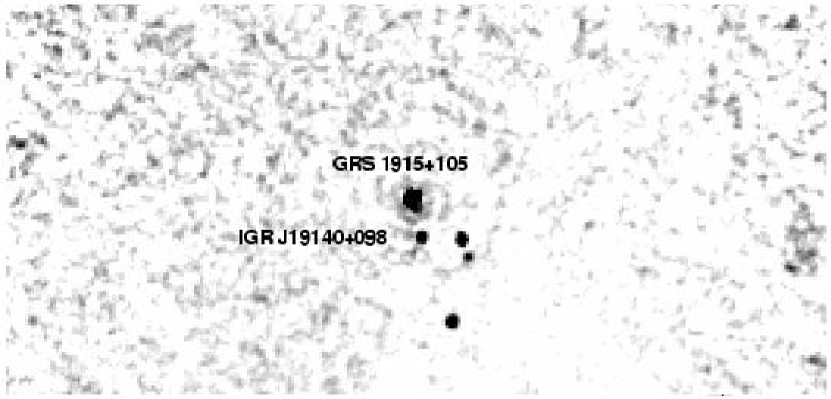
Figure 3: The IBIS/ISGRI 20–40 keV ($\sim 22^{\circ}$ width and $\sim 10^{\circ}$ height) image, showing the location of GRS 1915$+$105 and three other bright sources in the field, including the new transient IGR J1914$+$098 discovered during the observation of 2003 Mar 6. North is up and East is to the left.

Fig. 3 shows the IBIS/ISGRI 20–40 keV ($\sim 22^{\circ}\times\sim 10^{\circ}$) mosaicked image of the field of GRS 1915$+$105, with an exposure time of 98300 s. The elongation of the source is due to its apparent brightness in the mosaic. A preliminary background correction was performed (Terrier et al. 2003).

A new transient was discovered during the Rev. 48 observation, IGR J19140$+$098 (SIMBAD corrected name IGRJ 19140$+$0951; Hannikainen, Rodriguez & Pottschmidt 2003). See Schultz et al. (these proceedings), Cabanac et al. (2004) and Hannikainen et al. (in preparation) for details on this source.

Figure 4: The ISGRI lightcurves from Rev. 48. The 20–40 keV lightcurve (top) and the 40–80 keV lightcurve (bottom). The dashed line shows the 50 mCrab level in both energy ranges. The bin size is one science window, or 2200 s.

Fig. 4 shows that GRS 1915$+$105 was highly variable during Rev. 48. The dashed horizontal line in both panels indicates the 50 mCrab level in the given energy ranges. As can be inferred, the luminosity of the source varies between $\sim 30-100$ mCrab in the 20–40 keV range, and between $\sim 24-50$  mCrab in the 40–80 keV range.

Figure 5: Top. The JEM X-2 lightcurve from Rev. 48, showing how the source varied between 0.15 and 2 Crab. Bottom. A zoom of the JEM X-2 lightcurve showing the 5-min QPOs. The bin size is 8 s.

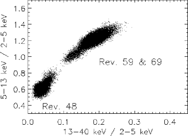
Figure 6: The RXTE/PCA color-color diagram for Revs. 48, 59 and 69. The time bin is 1s. The x- and y-scales correspond to those used for the $\chi$ classes in Fig. 2C in Belloni et al. (2000).

The Joint European X-ray monitor, JEM-X (Lund et al. 2003) consists of two identical coded mask instruments – however, during the time of these observations, only JEM X-2 was operational. Fig. 5 shows the JEM X-2 lightcurve from the whole of Rev. 48 (top), and a zoom covering 1.2 hours (bottom). As can be seen, the source was in a very variable state, with the flux varying between 0.25 to 2 Crab with a mean of $\sim 0.5$ Crab. The zoomed plot shows particularly striking rapid oscillations. Of particular interest are the main peaks separated by $\sim 5$ minutes. Although this kind of variability resembles the $\rho$-heartbeat, $\nu$ and $\phi$ oscillations (variability classes of Belloni et al. (2000)), these are more uniform and occur on shorter timescales. Recently, Tagger et al. (2004) have shown from a work of Fitzgibbon et al. (priv. comm.) that GRS 1915$+$105 seems to follow the same pattern of transition through all the 12 classes. This may suggest that GRS 1915$+$105 simply displays a continuum of all possible configurations and that we caught it in an intermediate class between two previously known ones. Our RXTE observations did not cover the entire 100 ks INTEGRAL data but were simultaneous. They confirm the variability seen by JEM X-2. We produced a color-color (CC) diagram for the RXTE data in the same manner as in Belloni et al. (2000) (note that the energy-channel conversion for PCA corresponds to epoch 5). The resultant plot is shown in Fig. 6. This CC-diagram and the JEM X-2 lightcurve seem to indicate a new type of variability not seen in the 12 classes by Belloni et al. (2000).

Fig. 7 shows the mean of nine RXTE/PCA pulses. As can be seen, the ‘ups’ were harder than the ‘downs’ – this behavior is opposite to that seen in the $\rho$, $\nu$ and $\phi$ oscillations. The rise is also faster than the decline. This type of behavior is very unusual for GRS 1915$+$105. In each case, there is a pre-flare not seen in the hard X-rays.

In order to have a first overview of the JEM X-2 capability in timing analysis, we carried out a Fourier Transform of the whole JEM X-2 lightcurves and obtained a power spectrum (Fig. 8). After removing artefacts due to some gaps in the data, we can identify a Quasi-Periodic Oscillation (QPO) at a frequency $3.32\times 10^{-3}$ Hz ($\sigma=3.6\times 10^{-4}$ Hz). At the current stage, the exact power of the feature cannot be known exactly since it requires a precise background estimate. The observation of such a low QPO with JEM X-2 is, however, of prime importance since it opens the studies of low frequencies (difficult to access with RXTE due to its 90-minute orbit, and usually shorter observations) through the long, continuous INTEGRAL observations. The frequency of this QPO is in agreement with the 5-minute timescale of the main peaks in the lightcurve. The fact that such a feature is detected from the Fourier transform of the whole 100 ks JEM X-2 lightcurve indicates that this class of variability is dominated by the 5-min oscillations. The power density spectrum was constructed for the whole 100 ksec of the observation and at times the oscillation disappears – hence the relative amplitude of the QPO is lower. A deeper analysis of the variability is in progress and will be published elsewhere. We conclude here that we have discovered a new type of variability in the JEM X-2 lightcurve of GRS 1915$+$105.

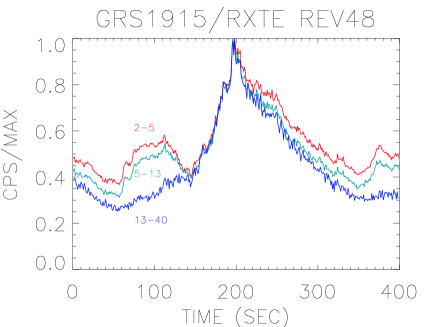
Figure 7: The mean of nine RXTE/PCA pulses (2–5 keV, 5–13 keV and 13–40 keV). The ‘ups’ are harder than the ‘downs’. The rise is faster than the decline, which is very unusual behavior for GRS 1915$+$105.

Figure 8: The JEM X-2 power spectrum. The QPO is at a frequency of 3.32$\times 10^{-3}$ Hz.

More on the timing analysis of GRS 1915$+$105 can be found in Rodriguez et al. (2004a, 2004b).

4 Revolutions 49 through 70

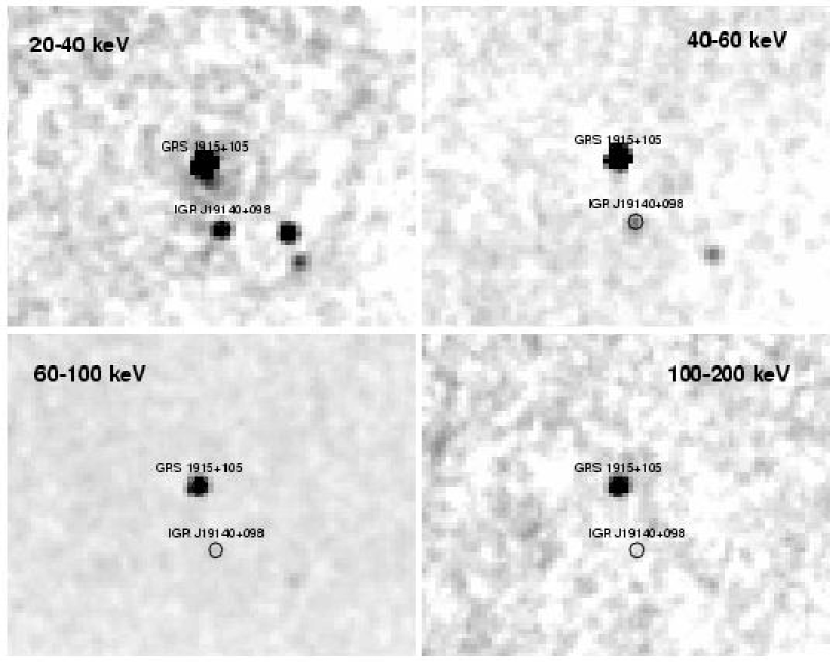
Figure 9: A mosaic from Revolutions 49, 51, 53, 56, 58, 59, 60, 69 and 70 in the 20–40 keV (top left), 40–60 keV (top right), 60–100 keV (bottom left) and 100–200 keV ranges (bottom right). The size of each image is approximately 6.15 (width) $\times$ 4.65 (height) degrees.

Figure 10: The JEM X-2 (top), ISGRI 20–40 and 40–80 keV (middle), and Ryle 15 GHz (bottom) lightcurves for Revs. 69 and 70. The JEM X-2 bin size is 500 s, while for ISGRI it is again one science window, ie 2200 s.

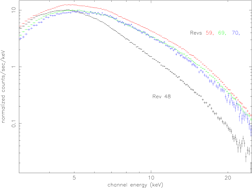
Figure 11: The JEM X-2 spectra from Revolutions 48, 59, 69 and 70. The figure shows how the spectrum from Rev. 48 is softer than those from Revs. 59, 69 and 70. However, one must bear in mind that the spectrum from Rev. 48 is in fact an average over the extreme variability observed during that revolution. For clarity, the systematic errors have been left out for this figure.

Fig. 9 shows the IBIS/ISGRI mosaicked image from revolutions 49, 51, 53, 56, 58, 59, 60, 69 and 70, in the 20–40 keV, 40–60 keV, 60–100 keV and 100-200 keV energy ranges. The figure shows that GRS 1915$+$105 is visible up to 200 keV. It also shows that the new source, IGR J19140$+$098, is clearly detected up the 60–100 keV range with a significance of 6.33$\sigma$.

Fig. 10 shows the lightcurves from revolutions 69 and 70 (Rev. 59 was omitted for clarity). The plot clearly demonstrates that the source was in a steady, “plateau” state, with a constant level of emission in the ISGRI and JEM X-2 energy ranges. One can also see that the radio emission is at the $\sim 50$ mJy level. This is characteristic of the $\chi$ state. More specifically, the level of radio emission allows us to identify the source as being in the $\chi 1-\chi 3$ state, ie a radio loud hard state (Muno et al. 2001), also known as the type II state (Trudolyubov 2001). For a comprehensive account of multiwavelength observations of the source in this state, see Fuchs et al. (2003) and Fuchs et al. (these proceedings).

Figure 6 shows the color-color diagram for Rev. 59 and 69. It is immediately evident that Revs. 59 and 69 are virtually identical to each other, and that they differ significantly from Rev. 48.

5 Spectral analysis

5.1 JEM X-2: Revs 48–70

Fig. 11 shows the JEM X-2 spectra from Revolutions 48, 59, 69 and 70. The spectrum from Revolution 48 is an average over the variability observed during that revolution. Data below 3 keV and above 25 keV were ignored. The spectra were fitted with an (absorbed) disk blackbody $+$ powerlaw $+$ Gaussian. Systematic errors of 20% were added up to energy 4 keV, 10% to the energy range 4–7 keV, and 2% in the range 7–25 keV. The results of the fits are shown in Table 2. The column density was fixed to $N_{H}=5\times 10^{22}\,{\rm cm}^{-2}$. A Gaussian of centroid 6.5 keV was needed for the fits in all four cases. The results show that during Rev. 48, the inner disk temperature was cooler than for the other revolutions. The luminosity of the source ranges from $8.0\times 10^{37}\,{\rm erg}\,{\rm s}^{-1}$ in Rev. 48, to $1.4\times 10^{38}\,{\rm erg}\,{\rm s}^{-1}$ in Rev. 59, based on a distance of 9 kpc (Chapuis & Corbel 2004).

Table 2: Results of the spectral fits to the JEM X-2 data.

Rev. #	$T_{in}$	$\Gamma$	$\chi^{2}_{\nu}$	Flux†
	(keV)			(3–20 keV)
48	$2.16^{+0.26}_{-0.20}$	$3.36^{+0.08}_{-0.08}$	0.93	0.822
59	$3.61^{+0.22}_{-0.20}$	$2.54^{+0.10}_{-0.09}$	0.70	1.461
69	$3.59^{+0.26}_{-0.21}$	$2.45^{+0.10}_{-0.09}$	0.66	1.178
70	$3.03^{+0.33}_{-0.21}$	$2.23^{+0.27}_{-0.35}$	0.82	1.117

^† $\times 10^{-8}$ erg cm^-2 s^-1

5.2 JEM X-2, ISGRI and SPI: Revs. 59–70

During Revs. 59 through 70, GRS 1915$+$105 was in a steady “plateau” state, as shown in Fig. 10 for Revs. 69 and 70. Figure 12 shows the resulting broadband spectrum obtained from JEM X-2, ISGRI and SPI. The discrepancy in the cross-calibration between SPI and the other two instruments, JEM X-2 and ISGRI, is a well-known fact and is taken into account by introducing a constant which is allowed to vary freely in the fitting procedure. The JEM X-2 spectrum is from Rev. 59, while the ISGRI spectrum is extracted from the mosaic image and the SPI spectrum is co-added from Revs. 59, 69 and 70. Energy ranges $<3$ keV and $>25$ keV were ignored in the JEM X-2 data, $<20$ keV in the ISGRI data and $>200$ keV in the SPI data.

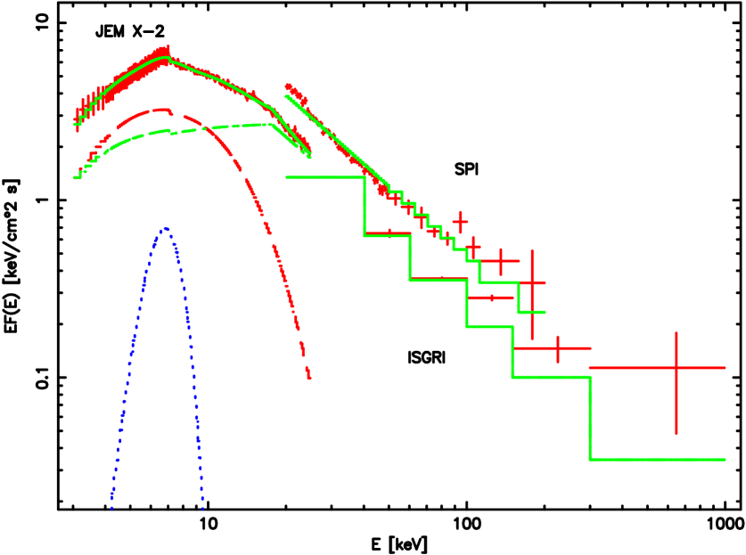
Figure 12: The INTEGRAL broadband spectrum: JEM X-2 + ISGRI + SPI.

Two models were fitted to the data, a simple broken powerlaw, and an (absorbed) disk blackbody + broken powerlaw + gaussian. Both fits yielded values comparable to those found by Trudolyubov (2001) for the Type II state. However, for the broken powerlaw only model, both the $\alpha_{1}$ and the break energy were slightly lower in our data, while in the disk blackbody + broken powerlaw the $\alpha_{1}$ was again slightly lower but the break energy was slightly higher. For the disk blackbody + broken powerlaw model a gaussian was needed, which was frozen to 6.5 keV. In both cases the column density was again fixed to $N_{H}=5\times 10^{22}\,{\rm cm}^{-2}$. In addition to the JEM X-2 systematics, overall systematics of 5% were added to the spectra. Table 3 shows the results of the fitting. Here we consider the simple broken powerlaw models for a direct comparison with Trudolyubov’s (2001) results. More physical models will be treated in future work. For now, it is tempting to consider that the origin of the second powerlaw may arise in the compact jet which is detected in the radio (for a discussion on the compact jet see Fuchs et al. 2003 and Rodriguez et al. 2004b). Fig. 2 shows that there is radio emission present throughout our observations at a fairly strong level, which most likely arises from the compact jet.

Table 3: Results of the spectral fits to the JEM X-2, ISGRI and SPI data.

Model	Broken powerlaw
$\alpha_{1}$	$2.07^{+0.06}_{-0.07}$
Break E (keV)	$9.98^{+0.43}_{-0.21}$
$\alpha_{2}$	$3.23^{+0.02}_{-0.03}$
$\chi^{2}_{\nu}$	1.40
Model	Disk blackbody + broken powerlaw
$T_{in}$ (keV)	$2.56^{+0.98}_{-0.16}$
$\alpha_{1}$	$1.99^{+0.50}_{-0.20}$
Break E (keV)	$17.63^{+3.28}_{-0.22}$
$\alpha_{2}$	$3.30^{+0.02}_{-0.05}$
$\chi^{2}_{\nu}$	0.85

6 Summary

We have presented INTEGRAL results from the first three months of monitoring of GRS 1915$+$105. We have shown that GRS 1915$+$105 exhibited two very distinct states during our observations: in Rev. 48 a new type of variability was discovered, while in Revs. 59, 69 and 70 the source was in the radio loud hard state (Muno et al. 2001), also known as the type II state (Trudolyubov 2001). Spectral fits to the JEM X-2, ISGRI and SPI data yielded parameters similar to those expected for the type II state, while spectral fits to the JEM X-2 data alone showed the source had a high inner disk temperature during the “plateau” states.

References

- Belloni et al. (2000) Belloni, T., Klein-Wolt, M., Méndez, M., van der Klis, M. & van Paradijs, J. 2000, A&A, 355, 271
- Cabanac et al. (2004) Cabanac, C., Rodriguez, J., Petrucci, P.-O., Henri, G., Hannikainen, D. & Durouchoux, P. 2004, astro-ph/0401308
- Castro-Tirado et al. (1992) Castro-Tirado, A.J., Brandt, S., & Lund, N. 1992, IAUC 5590
- Chapuis & Corbel (2004) Chapuis, C. & Corbel, S. 2004, A&A, 414, 659
- Cherepaschuk et al. (2003) Cherepaschuk, A.M., Sunyaev, R.A., Sefina, E.V., Panchenko, I.V., Molkov, S.V. & Postnov, K.A. 2003, A&A, 411, L441
- Courvoisier et al. (2003) Courvoisier, T. J. L., Walter, R., Beckmann, V., et al. 2003, A&A, 411, L53
- Fender et al. (1999) Fender, R.P., Garrington, S.T., McKay, D.J., et al., 1999, MNRAS, 304, 865
- Fuchs et al. (2003) Fuchs, Y., Rodriguez, J., Mirabel, I.F., et al. 2003, A&A, 409, L35
- Greiner et al. (2001) Greiner, J., Cuby, J.G., McCaughrean, M.J., Castro-Tirado, A. & Mennickent, R.E. 2001, A&A, 373, L37
- Hannikainen et al. (2003) Hannikainen, D.C., Vilhu, O., Rodriguez,J., et al. 2003, A&A, 411, L415
- Hannikainen, Rodriguez & Pottschmidt (2003) Hannikainen, D.C., Rodriguez, J.& Pottschmidt, K. 2003, IAUC 8088
- Harlaftis & Greiner (2004) Harlaftis, E. & Greiner, J. 2004, A&A, 414, L13
- Lund et al. (2003) Lund N., Budtz-Jørgensen C., Westergaard N.J., et al, 2003, A&A, 411, L231
- Mirabel & Rodríguez (1994) Mirabel, I.F. & Rodríguez, L.F. 1994, Nature, 371, 46
- Molkov et al. (2003) Molkov, S., Lutovinov, A. & Grebenev, S. 2003, A&A, 411, L357
- Morgan et al. (1997) Morgan, E.H, Remillard, R.A. & Greiner, J. 1997, ApJ, 482, 993
- Muno et al. (2001) Muno, M., Remillard, R., Morgan, E., et al., 2001, ApJ, 556, 515
- Paciesas et al. (1996) Paciesas, W.S, Deal, K.J., Harmon, B.A., et al. 1996, A&AS, 120, 205
- Rodriguez et al. (2004) Rodriguez, J., Fuchs, Y., Hannikainen, D.C., Vilhu, O., Shaw, S.E., Belloni, T. & Corbel, S. 2004a, astro-ph/0403030
- Rodriguez et al. (2004) Rodriguez, J., et al., 2004b, submitted to ApJ
- Tagger et al. (2004) Tagger, M., Varnière, P., Rodriguez, J. & Pellat, R., ApJ, in press, astro-ph/0401539
- Terrier et al. (2003) Terrier, R., Lebrun, F., Sauvageon, A., et al., 2003, A&A, 411, L167
- Trudolybov et al. (2001) Trudolyubov, S. 2001, ApJ, 558, 276
- Winkler et al. (2003) Winkler, C., Courvoiser, T.J.-L., DiCocco, G., et al. 2003, A&A, 411, L1
- Zdziarski et al. (2001) Zdziarski, A.A., Grove, J.E., Poutanen, J., Rao, A.R. & Vadawale, S.V. 2001, ApJ, 554, L45