Iron $K\alpha$ Fluorescent Line Profiles from Spiral Accretion Flows in AGNs

Abstract

We present 6.4 keV iron $K\alpha$ fluorescent line profiles predicted for a relativistic black hole accretion disk in the presence of a spiral motion in Kerr geometry, the work extended from an earlier literature motivated by recent magnetohydrodynamic (MHD) simulations. The velocity field of the spiral motion, superposed on the background Keplerian flow, results in a complicated redshift distribution in the accretion disk. An X-ray source attributed to a localized flaring region on the black hole symmetry axis illuminates the iron in the disk. The emissivity form becomes very steep because of the light bending effect from the primary X-ray source to the disk. The predicted line profile is calculated for various spiral waves, and we found, regardless of the source height, that: (i) a multiple-peak along with a classical double-peak structure generally appears, (ii) such a multiple-peak can be categorized into two types, sharp sub-peaks and periodic spiky peaks, (iii) a tightly-packed spiral wave tends to produce more spiky multiple peaks, whereas (iv) a spiral wave with a larger amplitude seems to generate more sharp sub-peaks, (v) the effect seems to be less significant when the spiral wave is centrally concentrated, (vi) the line shape may show a drastic change (forming a double-peak, triple-peak or multiple-peak feature) as the spiral wave rotates with the disk. Our results emphasize that around a rapidly-rotating black hole an extremely redshifted iron line profile with a noticeable spike-like feature can be realized in the presence of the spiral wave. Future X-ray observations, from Astro-E2 for example, will have sufficient spectral resolution for testing our spiral wave model which exhibits unique spike-like features.

1 Introduction

It is generally known that Seyfert 1s spectra exhibit reprocessed X-ray emission, such as broad Fe K$\alpha$ fluorescence at 6.4 keV and Compton reflection (high energy hump) around $\sim 30$ keV, from an illuminated accretion disk around a supermassive black hole. If the origin of such a reflection component can be attributed to a surrounding accretion disk (disk-line model), more precise spectral observations might allow us to better understand the physics in the vicinity very close to the central black hole. In standard disk-line models (Fabian et al., 1989; Laor, 1991; Kojima, 1991), accreting matter is normally considered to be in Keplerian orbit around a central black hole. The disk is then illuminated by an external X-ray source located somewhere near the innermost disk region and produces a broad, skewed fluorescent emission line at a particular photon energy (6.4 keV for neutral-like iron, 6.7 keV for He-like iron, and 6.9 keV for H-like iron, for instance) depending on the ionization state. See Fabian et al. (2002) and Reynolds & Nowak (2003) for comprehensive review.

Past X-ray observations with the Japan/USA X-ray satellite ASCA (the best resolving power of $\sim 120$ eV) revealed such a relativistically broadened iron line from various Seyfert 1 galaxies, particularly from a very bright source MCG-6-30-15 (Tanaka et al., 1995; Fabian et al., 1995). The observational data seems to be well-fitted with the standard disk-line model in terms of the characteristic double-peak feature, which is thought to be due to the longitudinal Doppler motion of the emitting matter in the disk, and the asymmetry in the profile is also believed to originate from the special relativistic, directional beaming effect. Furthermore, the observed emission line occasionally contains a very extended red tail that is interpreted to be a consequence of the general relativistic effect (i.e., gravitational redshift).

Apart from the standard disk-line models in which an axially symmetric flow with Keplerian circular motion is assumed under no perturbations, some authors have argued other accretion theories from different aspects. According to the past literatures, there seem to be three distinct issues of studies involved with such modifications: those (i) focusing on modified disk geometry instead of a simplified thin disk in the equatorial plane, (ii) more complex X-ray source geometry, and (iii) perturbed accretion flow (i.e., non-Keplerian flows). These issues (i)-(iii) seem to be independent of each other but they all modify the standard line profiles in terms of the redshift of photons, the line shape, and/or the line variabilities. As far as issue (i) is concerned, the actual disk geometry may not be so simple as geometrically-thin in the equatorial plane. For instance, Hartnoll & Blackman (2000) has discussed warping of the disk where a part of the disk surface is geometrically skewed and tilted from the equatorial plane. On the other hand, a thin disk might become hotter as the gas approaches the hole, forming a geometrically-thick disk (or an accretion torus). Such a thick disk model (accretion torus) has been studied by a number of authors, e.g., Shapiro, Lightman, & Eardley (1976), Tritz & Tsuruta (1989), and Kojima & Fukue (1992), while dense clouds embedded in a thick disk has been discussed by Guilbert & Rees (1988), Sivron & Tsuruta (1993) and Hartnoll & Blackman (2001). The second standpoint (ii) includes a stationary/dynamical, off-axis X-ray source (i.e., a non-axisymmetric point source) instead of a typically postulated axisymmetric X-ray source. That is, the primary source (for example, an orbiting flare in a corona or high energy particles due to shock accelerations) is either located off-axis or moving around with some bulk motion relative to the disk (Reynolds & Begelman, 1997; Ruszkowski, 2000; Dabrowski & Lasenby, 2001; Lu & Yu, 2001). A flaring activity induced in the disk itself might irradiate the Keplerian matter to produce iron fluorescence (Nayakshin & Kazanas, 2001). They found a very narrow line owing to the small height of the flare.

With regard to the third issue (iii), Keplerian motion may not be a very practical assumption since a thin disk is known to be subject to various kinds of instabilities to perturbations. For instance, disk oscillations can be triggered in the form of the (p,g,c)-mode in the innermost disk region (Kato, 2001a, b), in which case the local emissivity is no longer axisymmetric (Yamada & Fukue, 1993; Sanbuichi, Fukue, & Kojima, 1994; Karas, Martocchia, & Subr, 2001). Also, magnetohydrodynamic (MHD) instabilities such as the magneto-rotational instability (MRI) can induce spiral density waves in the presence of the magnetic field. This has been phenomenologically confirmed by two-dimensional numerical studies of a magnetized disk in Newtonian gravity where a multiple-armed spiral wave evolves into a single-armed spiral over some time (Caunt & Tagger, 2001, hereafter CT01). On the other hand, a recent three-dimensional MHD simulation of the black hole accretion by Machida & Matsumoto (2003, hereafter MM03) suggests that an X-ray flare via magnetic reconnections could take place in the plunging region (i.e., the region inside the marginally stable orbit) as a result of the non-axisymmetric (one-armed) spiral density structure, which is initially caused by MRI due to a differential rotation of frozen-in plasma. Hawley (2001, hereafter H01) has independently predicted a similar formation of tightly wrapped spiral waves using the Pseudo-Newtonian potential. It is also demonstrated by Armitage (2002) that the intensity of the magnetic fields in the accretion disk tends to be amplified by shearing, which could be a potential source of the observed X-rays. Additionally, a gravitational perturbation (tidal force) by a nearby star or a massive gas can trigger such a spiral wave which eventually steepens into shocks (Chakrabarti & Wiita, 1993a). The line profiles under such spiral patterns have been found by several authors (Chakrabarti & Wiita, 1993b, 1994) in the Newtonian geometry. In all these cases, the accreting flow is no longer Keplerian because of a substantial radial velocity component. Therefore, the velocity field should be somewhat deviated from a circular one. For instance, Hartnoll & Blackman (2002, hereafter HB02) considered the possible effects of such a spiral motion on the effective line profile in an approximate Schwarzschild geometry. HB02 found a quasi-periodic bump and many step-like features purely due to the velocity field of spiral waves. In their work, predicted profiles are obtained for various spiral wave parameters, and these authors concluded that the multiple sub-peaks are generally more prominent for larger spiral wave numbers.

In our current paper we will focus our attention on issues (ii) and (iii) where an X-ray source geometry and the velocity field are both important ingredients for determination of the iron line. Our model, being motivated by both HB02 and MM03, postulates a localized X-ray flare via a relatively small magnetic reconnection (small enough not to destroy the main structure) somewhere above the innermost region of the accretion disk around a rapidly-rotating black hole, in the presence of the spiral accretion flow superposed onto the background Keplerian motion, which is a different set-up from HB02. We also consider a different height of the flare. The X-ray flare will then illuminate the nearby disk material and produce cold iron fluorescent emission line at 6.4 keV in the rest frame. The iron is considered to be either neutral or only weakly ionized (i.e., Fe1-Fe16) in the case of a moderately weak flare. Thus, the effective iron line profile in our model will be determined primarily by both the spiral velocity field and the location of the flare.

The structure of this paper is as follows. In §2 we will introduce the assumptions made and establish our flare model in the context of the thin-disk line model in the presence of the spiral motion. The results are presented in §3 where we will show our theoretical line profiles for various situations including all the special/general relativistic effects, both from the flare source to the disk and from the disk to the observer. The apparent disk image (redshift and blackbody temperature) are also presented. The discussion and concluding remarks are given in the last section, §4.

2 Assumptions & Basic Equations

First, we construct a spiral motion, superimposed onto the unperturbed Keplerian orbit, in such a way that it qualitatively mimics to some degree the characteristic velocity field found in H01 and MM03. Then we introduce the geometry of our postulated flare X-ray source. For computing relativistic geodesics of emitted photons from the iron to the observer, the ray-tracing method is employed. All the general/special relativistic effects (longitudinal Doppler shift, relativistic beaming effect, bending of light, and the gravitational redshift) are included in our computations, both from the flare to the disk and from the disk to the flare.

2.1 Spiral Motion with the Keplerian Flow in the Disk

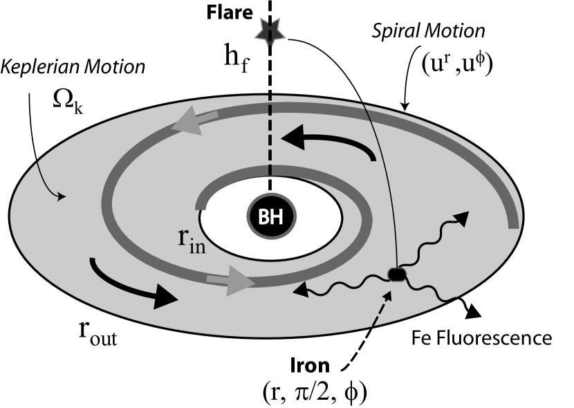
Figure 1: A cartoon of the the accretion disk in the presence of the spiral motion. The black hole is situated at the center above which an X-ray source (flare) is emitting primary photons. Not drawn to scale.

Let us first assume that the space-time is stationary ($\partial/\partial t=0$) and axially symmetric ($\partial/\partial\phi=0$) in the equatorial plane ($\theta=\pi/2$). Following the standard thin-disk models, the disk is considered to be geometrically-thin ($h/r\sim 0.1$) and optically-thick ($\tau_{es}>1$), ranging from an inner radius $r_{in}$ to an outer radius $r_{out}$. Here, $h$ is the scale-height of the thin disk, and $\tau_{es}$ is the electron scattering optical depth. The schematic geometry of our model is illustrated in Figure 1. It shows a schematic view of the innermost region along with a local flare at height $h_{f}$ above the disk surface at ($r,\pi/2,\phi$). The physical meaning of the illustrated notations will be explained in later sections.

The background geometry is described in the Boyer-Lindquist coordinates as

$$ds^{2} = -\left(1-\frac{2Mr}{\Sigma}\right)dt^{2}-\frac{4aMr\sin^{2}\theta}{\Sigma}\,dtd\phi$$ (1)

$$+\frac{A\,\sin^{2}\theta}{\Sigma}\,d\phi^{2}+\frac{\Sigma}{\Delta}\,dr^{2}+\Sigma\,d\theta^{2}\ ,$$

where $\Delta\equiv r^{2}-2Mr+a^{2},~{}\Sigma\equiv r^{2}+a^{2}\cos^{2},~{}A\equiv(r^{2}+a^{2})^{2}-a^{2}\Delta\sin^{2}\theta$, and $M$ and $a$ are the black hole mass and its specific angular momentum, respectively. The metric signature is $(-,+,+,+)$. Geometrized units are used such that $G=c=1$ where $G$ and $c$ are respectively the gravitational constant and the speed of light. In this paper, distance is normalized by the gravitational radius $r_{g}\equiv GM/c^{2}$. For instance, $r_{g}\sim 1.5\times 10^{12}$ cm for $10^{7}M_{\sun}$ black hole mass. The unperturbed accretion disk possesses the Keplerian accretion flow with the angular velocity $\Omega_{k}=1/(r^{3/2}+a)$ where $r$ is the position of the emitter (i.e., iron) in the disk surface. In order to discuss physical quantities let us introduce a zero angular momentum observer (ZAMO) in a locally non-rotating reference frame (LNRF) which is a locally flat space. As seen by a ZAMO, the physical three-velocity (radial and azimuthal components) of the unperturbed Keplerian flow is described by

$$v^{\hat{r}}_{k} = 0\ ,$$ (2)

$$v^{\hat{\phi}}_{k} = \frac{A}{\Sigma\Delta^{1/2}}(\Omega_{k}-\omega)\ ,$$ (3)

where $\omega\equiv 2aMr/A$ is the angular velocity of the ZAMO and the subscript “k” denotes the Keplerian value and $\hat{}$ (hat) represents quantities measured by the ZAMO. We set $r_{out}=30r_{g}$ in our calculations for two reasons. It is both because we are interested in the relativistic line broadening in the inner region of the disk and because our attention is focused on the broad redtail. The inner radius $r_{in}$ coincides with the marginally stable circular orbit at $r_{ms}$ below which the accreting flow starts spiralling-in towards the event horizon at $r_{h}$ along geodesics (free-fall with $u^{r}\neq 0$). Since the radial-gradient of the density within $r_{ms}$ (in the plunging region) is very large due to the free-fall trajectory, the optical depth $\tau_{es}$ there is not large enough to maintain the optically-thick assumption. Thus, we do not consider the accreting matter within $r_{ms}$ for fluorescence.

As suggested by H01 and MM03, the accretion disk is no longer Keplerian in the presence of magnetic fields because the field lines, which the accreting particles are frozen-in to, start interacting with one another. The MRI under a differential rotation is then expected to occur and trigger the perturbations on the otherwise ordered Keplerian flow. As a result, the density distribution starts appearing as an asymmetric, tightly wrapped spiral pattern. There could be multiple-armed spiral waves, but H01, MM03 and CT01 show that the spiral structure will eventually evolve into a single-armed pattern after a certain rotation period. For instance, in MM03 a one-armed spiral starts appearing at $t\sim 10t_{0}$ where $t_{0}$ is one orbital time at $r\sim 50r_{g}$, while CT01 has found a single-armed spiral pattern after about 200 orbits. Due to these findings by various previous authors, we only consider a one-armed spiral wave here. In H01, the specific angular momentum of the flow tends to fluctuate around the Keplerian value due to the MRI, and therefore we will phenomenologically include a similar effect caused by the spiral perturbations in the velocity. In order to qualitatively reproduce similar spiral motions found in their numerical results, we follow HB02 and use a simple representation of the bulk velocity field (radial and azimuthal components) of the spiral wave in the LNRF as

$$v^{\hat{r}}_{sw} = -A_{r}~{}e^{-(r-r_{in})/\Delta_{sw}}\sin^{\gamma_{o}}\left[k_{r}(r-r_{in})+m\phi/2-\phi_{sw}/2\right]\ ,$$ (4)

$$v^{\hat{\phi}}_{sw} = A_{\phi}~{}e^{-(r-r_{in})/\Delta_{sw}}\sin\left[k_{r}(r-r_{in})+m\phi-\phi_{sw}\right]\ ,$$ (5)

where the subscript “sw” denotes the spiral wave. Such a spiral motion can qualitatively mimic the velocity perturbation discovered by H01 and MM03, and hence it is not an arbitrary choice. The characteristic structure of the spiral motion is thus uniquely determined by a set of parameters $(A_{r},A_{\phi},m,k_{r},\Delta_{sw},\gamma_{o},\phi_{sw})$.

The number of parameters can be reduced by making reasonably acceptable assumptions in the following way. CT01 and MM03 both show that the azimuthal wave number $m$ is fixed to be $m=1$ for a single-armed spiral wave in a late stage of the spiral evolution. $\gamma_{o}$ determines the width of the spiral pattern and turns out to be ineffective to the qualitative features of the line profile. Therefore, it is held constant at $\gamma_{o}=2$. Given these fixed parameters, the actual free parameters are $(A_{r},A_{\phi},k_{r},\Delta_{sw},\phi_{sw})$. MM03 shows that the wave amplitude $A_{r}$ and $A_{\phi}$ are unlikely to be very large ($u^{r}$ only exceeds 0.1c). Besides, a large amplitude could perturb and destroy the whole disk structure. Therefore the amplitude is chosen to be relatively small ($A_{r}=A_{\phi}=0.1$) in most of our calculations in §3.1. However, we look for the possible effects of amplitude variations. $k_{r}$ characterizes a tightness (the number of winding) of the spiral pattern, and the effective (radial) range of the spiral motion is controlled by $\Delta_{sw}$. For instance, the spiral is more tightly packed when $k_{r}$ is large, and it is more centrally (i.e., radially inward) concentrated when $\Delta_{sw}$ is small. $\phi_{sw}$ denotes the phase of the spiral. $\phi_{sw}$ becomes an important factor for determining the line profile in the phase-dependent case. It is fixed otherwise. It is clear that the spiral motion is non-axisymmetric and dependent on its phase $\phi_{sw}$. To avoid the phase-dependence of the line profile, we hold the spiral phase constant, leaving us the few free parameters ($A_{r},A_{\phi},k_{r},\Delta_{sw}$), for specifying a spiral motion. However, we will later investigate the phase-evolved line profile holding every parameter fixed except for $\phi_{sw}$. Note that $\phi=270\arcdeg$ (equivalently $-90\arcdeg$) coincides with the observer’s azimuthal angle, and $v^{\hat{r}}_{sw}<0$ for accretion. $v^{\hat{r}}$ and $v^{\hat{\phi}}$ are set to be in-phase in equation (4) and equation (5), which turns out to be unimportant to the end results.

We assume that the effective accretion flow seen by a ZAMO in the LNRF is described as the sum of these velocity fields; the spiral orbit being superposed onto the unperturbed Keplerian orbit. By adding each physical three-velocity field in the LNRF, we get

$$v^{\hat{r}} = v^{\hat{r}}_{k}+v^{\hat{r}}_{sw}\ ,$$ (6)

$$v^{\hat{\phi}} = v^{\hat{\phi}}_{k}+v^{\hat{\phi}}_{sw}\ .$$ (7)

Since $(v^{\hat{r}},v^{\hat{\phi}})$ is not axisymmetric, the net velocity field is also non-axisymmetric. The corresponding four-velocity field of the effective flow is then written as

$$(u^{t},~{}u^{r},~{}u^{\theta},~{}u^{\phi})=u^{t}\left(1,~{}\frac{\Delta}{A^{1/2}}v^{\hat{r}},~{}0,~{}\frac{\Sigma\Delta^{1/2}}{A\sin\theta}v^{\hat{\phi}}+\omega\right),$$ (8)

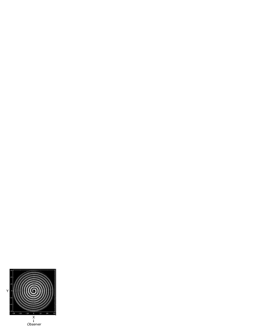
Figure 2: The spiral structure of the radial four-velocity component $u^{r}$ with $k_{r}=1.0,~{}\Delta_{sw}=30r_{g}$ and $A_{r}=A_{\phi}=0.1$. The inner disk region ($-30r_{g}\leq X\leq 30r_{g}$ and $-30r_{g}\leq Y\leq 30r_{g}$) is shown. A distant observer is situated in the azimuthal direction of $270\arcdeg$.

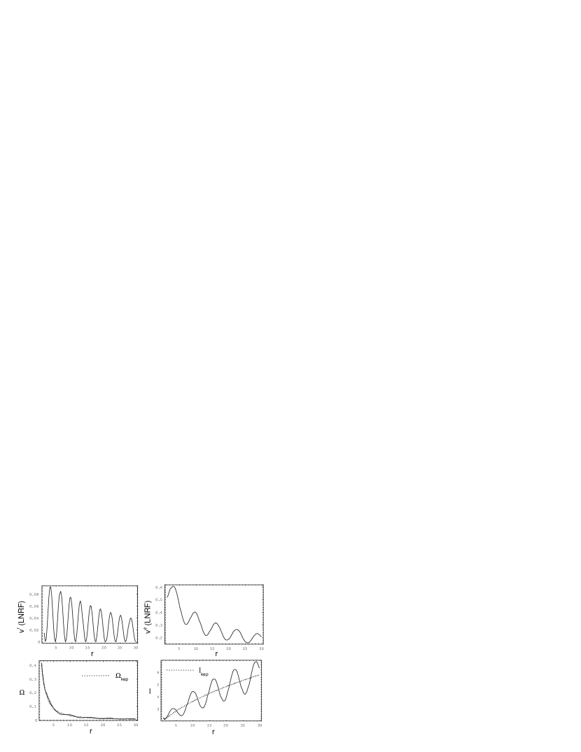
Figure 3: The velocity profiles corresponding to Figure 2. The radial three-velocity $v^{\hat{r}}$ (upper-left) in LNRF, the azimuthal three-velocity $v^{\hat{\phi}}$ (upper-right) in LNRF, the effective angular velocity $\Omega$ (lower-left) and the specific angular momentum $\ell$ (lower-right) are respectively displayed along the X-axis ($\phi=0\arcdeg$) for $k_{r}=1.0,~{}\Delta_{sw}=30r_{g}$ and $A_{r}=A_{\phi}=0.1$. The dotted curves are for the unperturbed Keplerian orbit.

where $u^{t}=[-\hat{V}^{2}\Delta\Sigma/A+1-2r/\Sigma+A\omega^{2}/\Sigma]^{-1/2}$ and $\hat{V}^{2}\equiv(v^{\hat{r}})^{2}+(v^{\hat{\phi}})^{2}$ is the square of the physical three-velocity of the perturbed flow in the LNRF. $\omega\equiv 2Mar/A$ is the angular velocity of the ZAMO with respect to a distant inertial frame. Thus, the effective velocity field including the spiral motion in Keplerian background orbit is determined once we specify $v^{\hat{r}}_{sw}$ and $v^{\hat{\phi}}_{sw}$ through a set of free parameters $(A_{r},A_{\phi},k_{r},\Delta_{sw})$. Figure 2 shows an example of a perturbed accreting flow where the radial four-velocity component $u^{r}$ described by equation (8) is plotted in the equatorial plane ($-30\leq X\leq 30$ and $-30\leq Y\leq 30$). The adopted parameters are $k_{r}=1.0,~{}\Delta_{sw}=30r_{g}$ for illustration purpose. The corresponding velocity profile at $\phi=0\arcdeg$ (along Y=0 in Figure 2) is shown in Figure 3. From upper-left clockwise, the radial three-velocity $v^{\hat{r}}$, the azimuthal three-velocity $v^{\hat{\phi}}$, the effective angular velocity $\Omega$ and the specific angular momentum of the gas $\ell$ are displayed, respectively. For comparison, the dotted curves are also shown for Keplerian motion.

2.2 A Localized X-ray Flare Source

In our model the X-ray flare source is a locally stationary active region (e.g., flaring sites in corona) at some height $h_{f}$ on the symmetry axis above the innermost disk. Following the practice adopted in many standard disk-corona model for the Fe fluorescent lines, we also approximate such a source as a point-like X-ray source on the black hole symmetry axis (see Figure 1). This assumption should be justified because the hottest region should be above the innermost disk because the multi-color disk temperature scales as $\propto r^{-3/4}$. That should be very close to the rotation axis of the hole. We also assume that the entire disk is neutral or at most only weakly ionized by such a radiation source, producing a neutral-like fluorescence at $6.4$ keV in the source frame. In this manner we can investigate the effects exclusively due to the spiral wave alone, by comparing our results with those obtained for the standard Keplerian disk model without spiral waves.

2.3 Relativistic Disk Emissivity

In Newtonian geometry, specifying the height of the X-ray source $h_{f}$ would simply allow us to compute the emissivity law of the illuminated disk. In addition, it is also important, especially in the innermost region in the relativistic disk, to take into account the general relativistic bending effect (either redshift or blueshift) on the photons from the flare to the disk. Due to this effect, the intensity of the illuminating photon flux at the disk should be subject to a significant deviation from the Newtonian case. Reynolds & Begelman (1997) calculated this effect for their iron lines predicted for Schwarzschild geometry, whereas Martocchia & Matt (1996) calculated the photon trajectories from an on-axis source to the underlying accretion disk in Kerr geometry. We adopt and modify the work of the latter authors who found the redshift factor $g_{sd}$ measured in a local disk frame (i.e., ZAMO) as

$$g_{sd}=\sqrt{\frac{(r^{2}+a^{2}-2r)(r^{2}+a^{2}+2a^{2}/r)}{(1-\hat{V}^{2})(r^{2}+a^{2}-2r)(h^{2}_{f}+a^{2})}},\$$ (9)

where we adopt the extreme Kerr parameter $a=0.998$ according to recent theoretical/observational speculations that a black hole is likely to rotate rapidly in some AGNs (Iwasawa et al., 1996a, b; Young, Ross, & Fabian, 1998; Fabian et al., 2002; Wilms et al., 2001). Given the canonical photon power-law index ($\Gamma_{PL}\sim 1.9$) for Seyfert 1s (Nandra & Pounds, 1994), the actual local emissivity is weighted by the factor of $g^{1.9}_{sd}$, which yields the net local axisymmetric emissivity as

$$\tilde{\epsilon}_{d}=\epsilon_{d}~{}g^{1.9}_{sd}\ ,$$ (10)

where $\epsilon_{d}$ is the local Newtonian emissivity of the disk expressed as

$$\epsilon_{d}=\frac{h_{f}}{\left(r^{2}+h_{f}^{2}\right)^{3/2}}\ .$$ (11)

Here, $r$ is the radial position of the emitter (iron) in the disk.

2.4 Photon Trajectories

When fluorescent photons emitted from the disk reach a distant observer or telescope, the following geodesic equation in the integral form must be satisfied (Carter, 1968; Chandrasekhar, 1983):

$$\int_{r_{em}}^{r_{obs}}{{1\over\sqrt{R(r)}}\,dr}=\pm\int_{\theta_{em}}^{\theta_{obs}}{{1\over\sqrt{\Theta(\theta)}}\,d\theta}\ ,$$ (12)

where

$$R(r,\lambda,Q) = r^{4}+(\lambda^{2}-Q)^{2}+2(Q+\lambda^{2})r-Q,$$ (13)

$$\Theta(\theta,\lambda,Q) = Q-(\lambda\cdot cot\theta)^{2},$$ (14)

Here an observer’s distance $r_{obs}$ and its inclination angle $\theta_{obs}$ need to be specified. $(r_{em},\theta_{em})$ is the emitter’s (i.e., iron) position on the disk. For a distant observer, we take $r_{obs}=\infty$. $\lambda$ and $Q$ are two constants of motion along a geodesic, which are closely related to the axial component of the angular momentum of photons Carter (1968). We will make full use of the elliptic integrals to numerically evaluate equation (12) in the ray-tracing approach (Cadez, Fanton, & Calvani, 1998; Fanton et al., 1997) for efficient computations. We will first search for an observable photon emitted from $r_{em}$ in the disk, and then calculate the corresponding redshift $g_{do}$. Given the 4-velocity of the perturbed flow (iron) and the 4-momentum of the null geodesic (photon), we obtain the redshift by

$$g_{do}\equiv\frac{E_{obs}}{E_{em}}=1/[u^{t}(1-\lambda\Omega-v^{\hat{r}}\sqrt{R}/r^{2})]\ ,$$ (15)

where the observer at a distant location $r_{obs}$ is stationary. $E_{em}$ and $E_{obs}$ are the local photon energy and its observed energy, respectively. We consider a photographic plate of the observer’s (or telescope’s) window at $r_{obs}$ facing straight the accretion disk with the inclination angle $\theta_{obs}$. Images of the disk are projected onto this window with ($\alpha,\beta$) where $\alpha,\beta$ are the impact parameters of the observed photons in observer’s sky. In our calculations, the window roughly contains $280\times 280$ pixels (corresponding to the spatial resolution of $\sim 0.23r_{g}$) in which the images of the disk are generated in false color. We only consider the observed photons normal to this window.

2.5 Predicted Fluorescent Emission Lines

Once we know the redshift factor $g_{do}$ and the surface emissivity of the disk $\epsilon_{d}$ including the bending effect expressed by $g_{sd}$, the observed photon flux is obtained by

$$F_{obs}(E_{obs})=\int_{source}g_{do}^{4}~{}I_{em}~{}d\Omega,$$ (16)

where d$\Omega$ is the solid angle subtended by the disk in the observer’s frame. Here, the local intensity is approximated by the $\delta$-function of the monochromatic photon energy $E_{em}$ in the source frame as $I_{em}=\tilde{\epsilon}_{d}\cdot\delta(E_{obs}-E_{em})$. Broadening of the line photons due to turbulence may be insignificant (Fabian et al., 2000). The local emitting region is assumed to be optically thick in the absence of a thick electron-scattering atmosphere above the disk so that the limb-darkening effect is unimportant, especially for a small inclination angle $\theta_{obs}$(Chen & Eardley, 1991; Laor, 1991; Bao, Hadrava, & Ostgaard, 1994). In a statistical sense, it seems to be favored that the averaged $\theta_{obs}$ for Seyfert 1s is around $\sim 30\arcdeg$ (Antonucchi & Miller, 1985; Schmitt et al., 2001). Therefore, we adopt $\theta_{obs}=30\arcdeg$ throughout this paper. Notice that the additional redshift factor $g_{sd}$ due to the photon bending (from the source to the disk plane) is included via our emissivity prescription $\tilde{\epsilon}_{d}$ in the modified local intensity $I_{em}$.

Using the obtained fluorescent flux, we can estimate the equivalent blackbody temperature measured by a distant observer $T_{obs}$ from the Stefan-Boltzmann law

$$T_{obs}=(F_{obs}/\sigma_{SB})^{1/4}\ ,$$ (17)

which is a function of the redshift factor $g_{do}$, the position of the emitter in the disk $(r,\pi/2,\phi)$ for a given height of the flare $h_{f}$. $T_{obs}$ will allow us to see the temperature distribution in the perturbed disk. If the spiral wave is fixed in the rotating disk frame, the line profile becomes phase-dependent of $\phi_{sw}$, and its characteristic rotational period should be the Keplerian value.

3 Results

Since there are a few degrees of freedom in our parameter space that primarily characterize the line shape, we need to carefully and systematically examine the effects of each parameter alone. First, we will see the effects of various spiral patterns by varying ($k_{r},~{}\Delta_{sw}$) for a given spiral phase $\phi_{sw}=0\arcdeg$. Later in §3.1.2, the spiral phase $\phi_{sw}$ is varied under the assumption that the spiral structure is fixed in the rotating disk frame. Our primary goal in the present paper is to demonstrate any detectable features seen in the iron line exclusively caused by a spiral perturbed velocity field, but for comparison purpose let us consider two different source height: $h_{f}=4r_{g}$ (a flare close to the hole) and $h_{f}=10r_{g}$ (a relatively distant flare). The selected parameters for various models are tabulated in Table 1. In all cases we set $A_{r}=A_{\phi}$ (equal amplitude) unless otherwise stated.

3.1 Predicted Iron Line Profile

Using the ray-tracing method, we are able to find roughly $\sim 6\times 10^{4}$ photon trajectories between the accretion disk and the observer. In the subsequent binning process for various photon energy, we set the spectral resolution to be $E/\Delta E\sim 600$, equivalent to $\sim 10$ eV, which can be achieved with X-ray Spectrometer (XRS) on board Astro-E2. We will first show the dependence of the wave pattern ($A_{r},A_{\phi},k_{r},\Delta_{sw}$) in §3.1.1. Lastly, in §3.1.2 we will explain the phase-dependence of the profile.

3.1.1 Effects of Various Spiral Motions

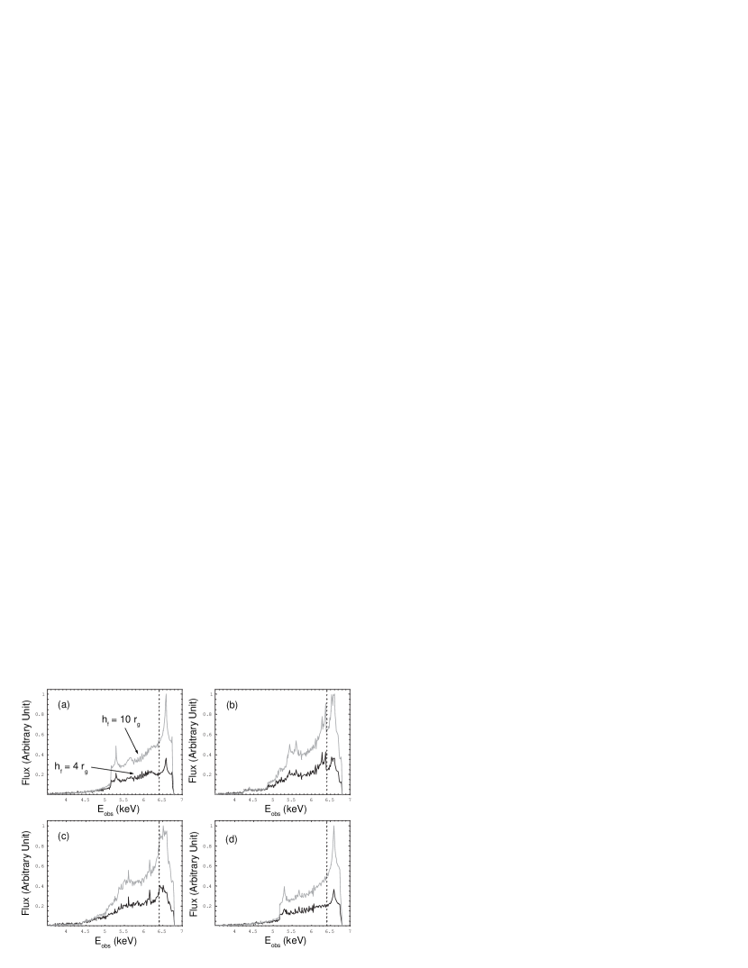
Figure 4: The predicted iron line profiles for various $k_{r}$ with $\Delta_{sw}=30r_{g}$. $k_{r}=0.4,~{}1.0,~{}1.5$ and $0.4$ for (a), (b), (c) and (d), respectively. $A_{r}=A_{\phi}=0.1$ in all cases but (d) where $A_{r}=0.1A_{\phi}=0.01$. A different source height is considered: a nearby-source ($h_{f}=4r_{g}$) in the dark curve and a distant source ($h_{f}=10r_{g}$) in the light grey curve. The spectral resolution $E/\Delta E$ is $\sim 600$ (corresponding to $\sim 10$ ev) achievable with Astro-E2 XRS. The vertical dotted line denotes 6.4 keV line in the rest frame.

Figure 4 shows the predicted line profiles for various $k_{r}$ with $\Delta_{sw}=30r_{g}$. The horizontal axis shows the observed photon energy in keV while the vertical axis denotes the observed photon flux in an arbitrary unit. $k_{r}=0.4,~{}1.0$ and $1.5$ for (a), (b) and (c), while in (d) $k_{r}=0.4$ but $A_{r}=0.1A_{\phi}=0.01$ in order to see $v^{\hat{r}}$-dependence. The dark solid curve represents the case where $h_{f}=4r_{g}$ while the light grey curve denotes the case with $h_{f}=10r_{g}$. The vertical dotted line shows a cold fluorescent line at 6.4 keV in the rest frame. In general, randomly formed sub-peaks are present due to the spiral velocity field, consistent with HB02. We further discover that there are normally two types of peaks existing in the profile: (i) relatively sharp sub-peaks and (ii) very spiky quasi-periodic multiple-peaks. The two kinds of peaks are in general simultaneously formed and are distinguishable in many cases, which is a new result inherent to our model. The spike-like features (ii) seem to be more prominent as $k_{r}$ increases because the winding of the spiral arm is amplified although the sharp sub-peaks (i) are less obvious. We can clearly observe an unusual double-peak structure (or a quasi-triple-peak structure) in (a). As $k_{r}$ becomes larger, quasi-periodic spike-like peaks tend to dominate over the sharp peaks, smoothing out the (classical) prominent peaks. When the spiral wave is tightly packed ($k_{r}=1.5$), the profile seems to become almost monotonic in the sense that the sharp sub-peak structure described as (i) is no longer clearly formed and instead be dominated by spiky multiple-peaks classified as (ii). This is justified from another model with $k_{r}=2.0$ (not shown here). The radial velocity component $v^{\hat{r}}$ appears to be unimportant (or relatively insignificant) in the qualitative formation of the randomly distributed peaks. The flux with a distant X-ray source ($h_{f}=10r_{g}$) is larger than that with a nearby source ($h_{f}=4r_{g}$) at most of the energy $E_{obs}$ band. This can be understood by the fact that for $h_{f}=4r_{g}$ the emissivity form $\tilde{\epsilon}_{d}$ becomes extremely centrally-concentrated because of a huge effect of light bending via $g_{sd}$, which yields a very steep emissivity in the innermost region. In this case, the innermost gas with a high redshift factor (hence emitting low energy photons) plays an important role in producing the iron line, which has almost no significant contributions to high energy fluorescent photons. In the case of $h_{f}=10r_{g}$, on the other hand, the bending of light is not as crucial as the previous case, and therefore such a relatively distant X-ray source can illuminate the whole disk (gas) in an even manner to produce more flux of blueshifted photons.

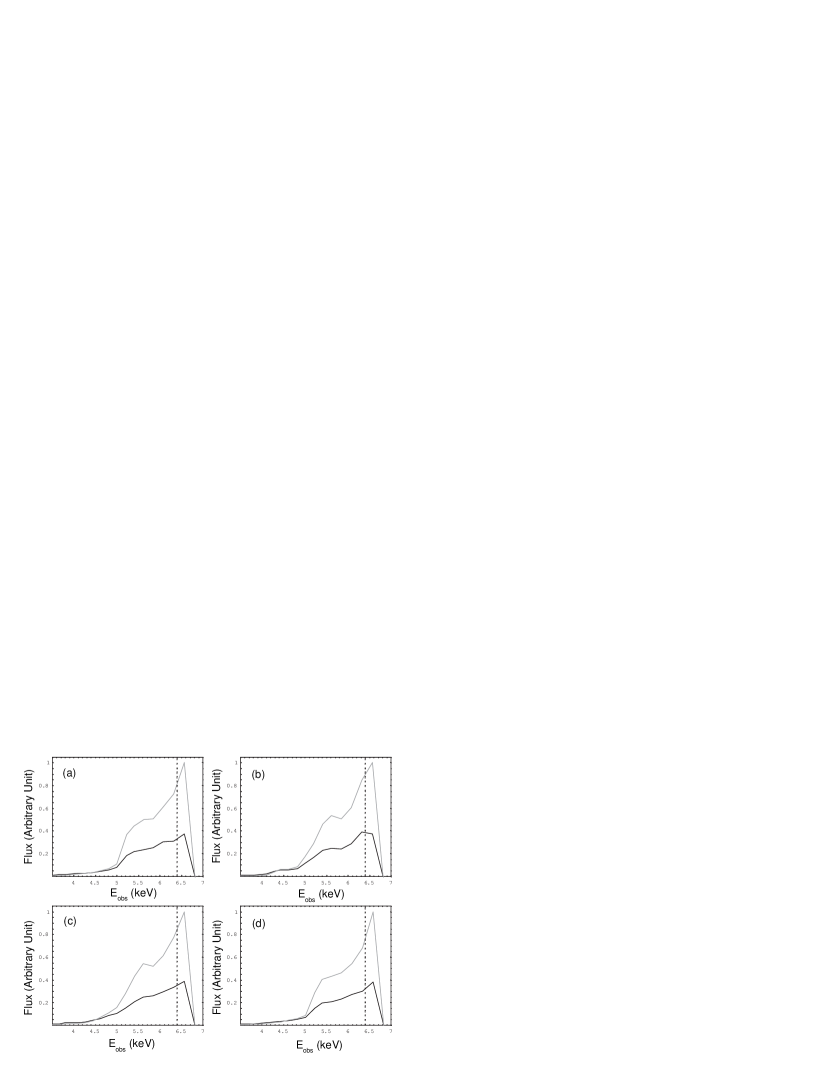
Figure 5: The predicted iron line profiles with the same parameter sets as in Figure 4 except that the spectral resolution $E/\Delta E$ is $\sim 50$ (corresponding to $\sim 120$ eV) already achieved with ASCA.

To better illustrate an observational difference associated with a currently available spectral resolution, the same line profiles are obtained with $E/\Delta E=50$ (corresponding to $\sim 120$ eV already achieved with ASCA) in Figure 5 where for comparison the same parameter sets are adopted as in Figure 4. With such an energy resolution, it seems very difficult to differentiate one model from the other (for instance, the one with low $k_{r}$-value and the one with high $k_{r}$-value) and even impossible to distinguish the present model (with perturbations) from the standard disk-line model. This, however, will be distinguishable observationally with a much better spectral resolving power that should be available in the next generation X-ray telescopes such as Astro-E2.

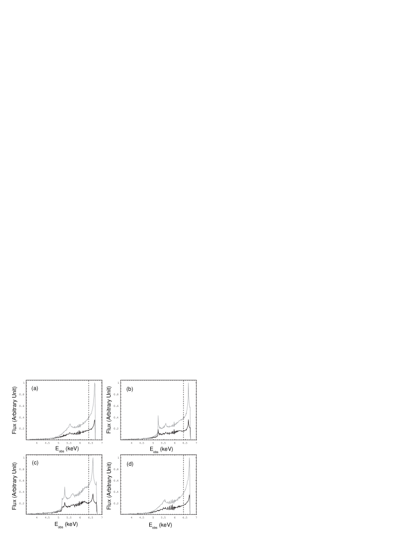
Figure 6: The predicted iron line profiles for various $\Delta_{sw}$ with $k_{r}=0.4$. $\Delta_{sw}/r_{g}=5,~{}15,~{}30$ and $5$ for (a), (b), (c) and (d), respectively. $A_{r}=A_{\phi}=0.1$ in all cases but (d) where $A_{r}=0.1A_{\phi}=0.01$.

Figure 6 displays the profiles for various $\Delta_{sw}$ with $k_{r}=0.4$ where $\Delta_{sw}$ determines the effective (radial) distance of the spiral perturbation. We use $\Delta_{sw}/r_{g}=5,~{}15$ and $30$ for (a), (b) and (c), respectively, while in (d) we adopt $\Delta_{sw}/r_{g}=5$ and $A_{r}=0.1A_{\phi}=0.01$. The degree of the spiky multiple-peak looks roughly unchanged in every case regardless of $\Delta_{sw}$, and those multiple-peaks are already present even when the spiral is centrally concentrated in (a). However, the overall line shape in (a) is similar to that of the standard model in terms of the double-peak structure (the third peak between the red one and the blue one is almost unseen). Therefore, it may be difficult to detect significant spiral effects when the perturbation is concentrated radially-inward. Again, the radial component of the spiral motion appears to be unimportant in this case, too.

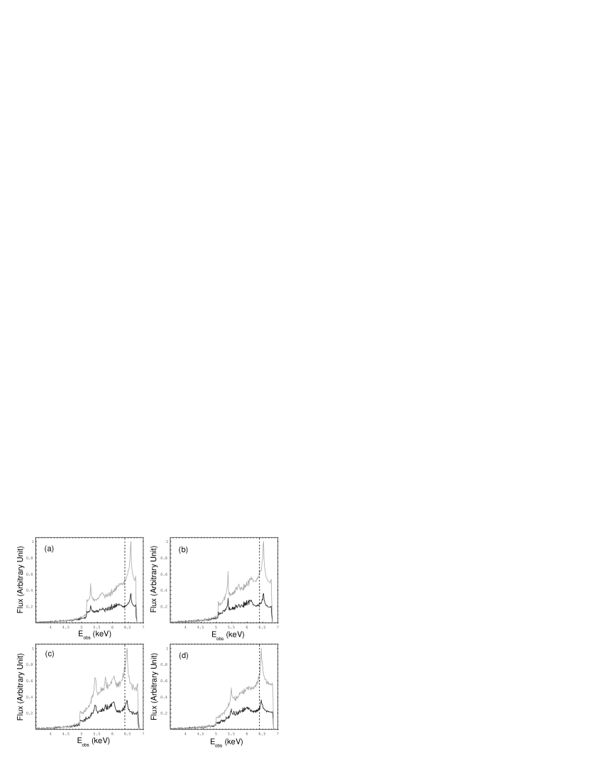
Figure 7: The predicted iron line profiles for various amplitude ($A_{r},A_{\phi}$) with $k_{r}=0.4$ and $\Delta_{sw}=30r_{g}$. $A_{r}=A_{\phi}=0.1,~{}0.15$ and $0.2$ for (a), (b) and (c), respectively. In (d), $A_{r}=0.1A_{\phi}=0.02$.

As we earlier mentioned, more effects of the spiral motion is intuitively expected when the amplitude is large. In Figure 7, $A_{r}=A_{\phi}=0.1,~{}0.15$ and $0.2$ in (a), (b) and (c), respectively while in (d) $A_{r}=0.1A_{\phi}=0.02$. As expected, a large amplitude tends to complicates the line shape more effectively. Specifically, the number of sharp sub-peaks appears to increase whereas the degree of the spiky multiple-peaks remains almost unchanged when the amplitude increases. For example, the number of sub-peaks can be as high as $\sim 6$ when $A_{r}=0.2$ in (c) while it is $\sim 3$ when $A_{r}=0.1$ in (a). For a small radial component in (d), there seems to be no significant difference from (a).

From what we find so far, it seems reasonable to say that the resulting line profile can be made very different from the classical one basically in two ways: (1) a tightly packed spiral wave with large $k_{r}$ tends to produce more spiky multiple-peaks (wiggling) or (2) a large azimuthal amplitude $A_{\phi}$ tends to produce more sharp sub-peaks, unless the spiral wave is restricted to the very inner region (small $\Delta_{sw}$).

3.1.2 Phase-Dependence

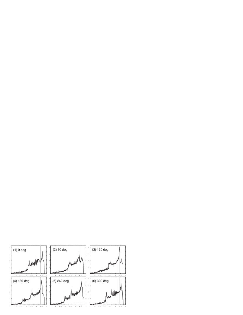
Figure 8: The phase-evolved iron line profiles from a spiral wave with $k_{r}=0.4,~{}\Delta_{sw}=30r_{g}$ and $A_{r}=A_{\phi}=0.1$. The source height is at $h_{f}=4r_{g}$. The phase of the spiral wave $\phi_{sw}$ is progressing from (1) $0\arcdeg$ to (6) $300\arcdeg$ by $60\arcdeg$. The horizontal axis is the observed photon energy $E_{obs}$ (keV) while the vertical axis shows the observed photon flux in arbitrary units.

In Figure 8 we show the phase-dependence of the line profiles for a fixed spiral structure, with $k_{r}=0.4,~{}\Delta_{sw}=30r_{g}$ and $A_{r}=A_{\phi}=0.1$, varying $\phi_{sw}$ from $0\arcdeg$ to $300\arcdeg$ by $60\arcdeg$. The source height is $h_{f}=4r_{g}$. The spiral wave is now fixed to the rotating disk frame. In other words, the spiral is corotating with the accreting gas. The distant observer at $r_{obs}\sim\infty$ is situated at $270\arcdeg$ (or equivalently $-90\arcdeg$) in its azimuthal position.

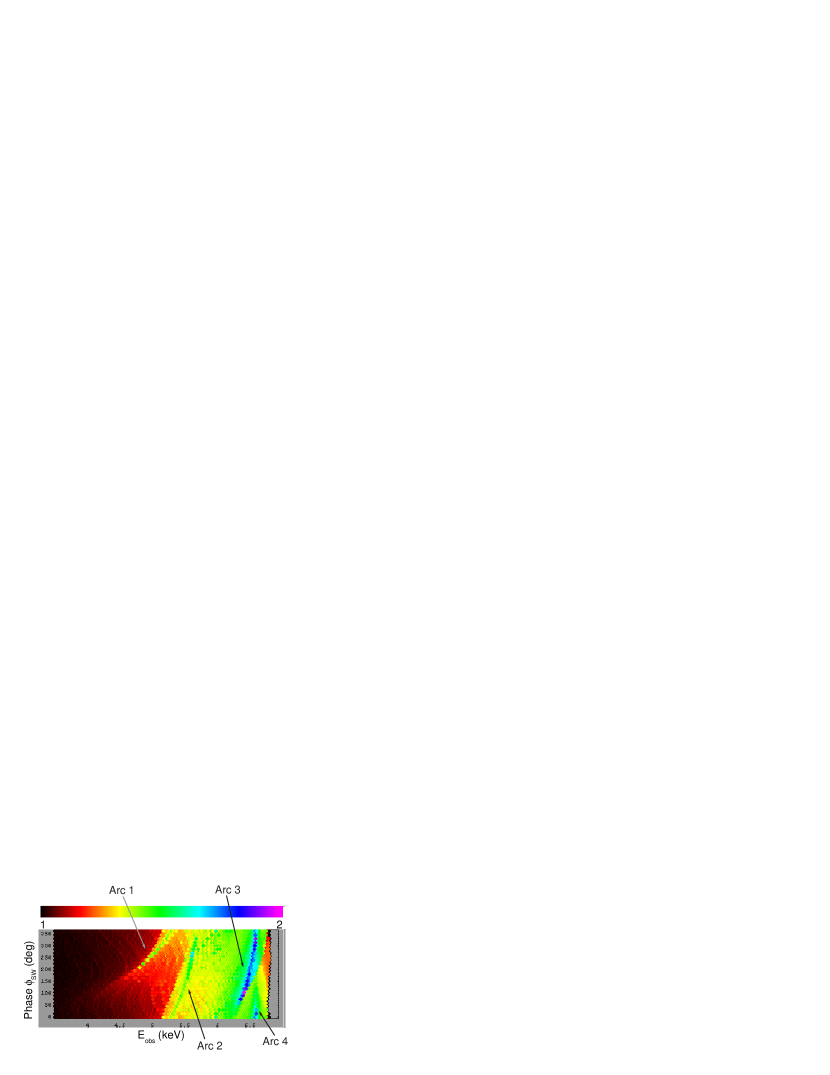
Figure 9: The intensity map of the global evolution of the iron line in the energy-phase $E_{obs}-\phi_{sw}$ space corresponding to Figure 8 with the same parameter set being used. The phase of the spiral wave $\phi_{sw}$ is progressing from $0\arcdeg$ to $345\arcdeg$ by $15\arcdeg$.The intensity is normalized between 1 and 2. [A color version of this figure is available at the electronic edition of the Journal.]

First of all, the profile appears to be constantly broadened over the photon energy $E_{obs}$ ($\gtrsim$ 4 keV) for the entire phase of the spiral wave $\phi_{sw}$ probably due to a small radius of the marginally stable orbit $r_{ms}$. The line shape also normally contains a triple-peak structure (left-end peak, middle-peak and right-end peak) with the dominating blue peak (or right-end peak) at all the times. It can be classified as belonging to roughly two categories depending on its characteristic shape: (i) the left-end peak above 5 keV such (1), (2), (3) and (6) and (ii) the left-end peak below 5 keV such as (4) and (5). The line energy of each peak then shifts towards either higher energy or lower energy depending on the phase $\phi_{sw}$ (i.e., peak transition). This trend can be viewed in relation to the spiral phase $\phi_{sw}$ in the following. The main cause of this complicated variation primarily originates from the fact that some parts of the accretion disk is more redshifted while the other parts, on the other hand, are more blueshifted depending on the phase $\phi_{sw}$. Hence, non-axisymmetry in the net velocity field is directly responsible for producing such a variability for a fixed X-ray source $h_{f}$. As discussed earlier, a choice of nearby source (smaller $h_{f}$) tends to generate more frequent sub-peaks due to more exclusive contribution from the innermost gas where the spiral perturbation is greater. On the other hand, spiky quasi-periodic peaks do not seem to change very much over the phase $\phi_{sw}$. We have also confirmed that the above variation (or the transition of peaks) with phase $\phi_{sw}$ is not so obvious when $k_{r}$ is large because the velocity field becomes somewhat quasi-axisymmetric (that is, the perturbation becomes more or less uniform everywhere). Hence, the noticeable line variability would be more expected when the perturbing spiral wave is not so tightly packed (i.e., small $k_{r}$). The corresponding global variation with $\phi_{sw}$ can also be seen in Figure 9 where the normalized line intensity is plotted as a function of the observed photon energy $E_{obs}$ (in keV) and the spiral phase $\phi_{sw}$ (in degrees), corresponding to Figure 8. [A color version of this figure is available at the electronic edition of the Journal.] The intensity is normalized between 1 (its minimum) and 2 (its maximum). An interesting pattern here is the existence of four distinct “arcs (i.e., the transition of peaks)” present at different energy $E_{obs}$: arc 1 ($E_{obs}\sim 4.5-5.3$ keV), arc 2 (5.3-5.7 keV), arc 3 (6.3-6.5 keV) and arc 4 ($\sim$ 6.6 keV), respectively. They individually correspond to the sharp peaks seen in the Figure 8. Besides such arcs, a randomly-distributed, wiggling variation of the line intensity is clearly present, especially at $E_{obs}\sim 6$ keV, due to the perturbed velocity field. This corresponds to the quasi-periodic multiple-peaks in Figure 8.

3.2 Redshift & Temperature Distribution

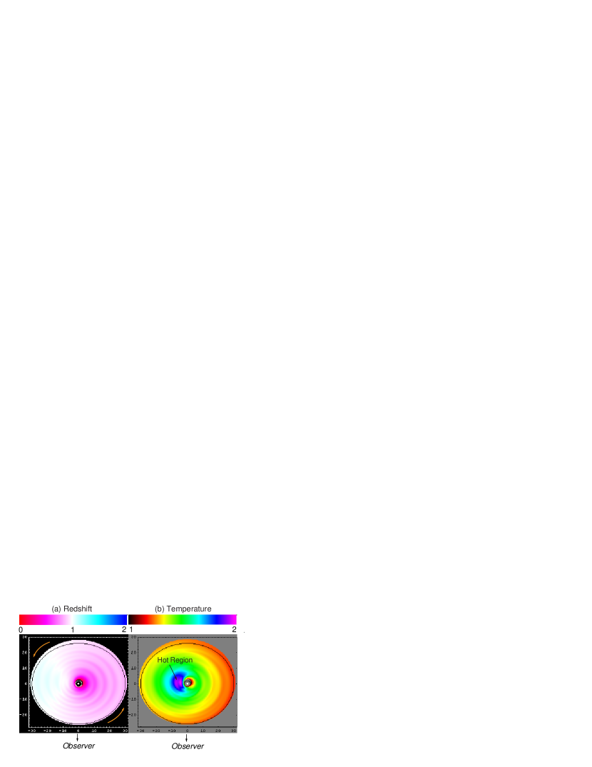
Figure 10: The redshift distribution $g_{do}$ of the emitted photons in the disk (left panel) and the equivalent blackbody temperature distribution $T_{obs}$ of the disk (right panel) for $k_{r}=1.0,~{}\Delta_{sw}=30r_{g}$, and $A_{r}=A_{\phi}=0.1$. The phase of the spiral is $\phi_{sw}=0$ and the source is at $h_{f}=4r_{g}$. A distant observer is situated in the direction of $270\arcdeg$ (or equivalently $-90\arcdeg$). The redshift $g_{do}$ of the observed photons is scaled between 0 and 2 in the left panel while the apparent disk temperature $T_{obs}$ is normalized between 1 and 2 in the right panel. The inner circle denotes the event horizon $r_{h}$ while the outer circle denotes the Newtonian circle with the radius of $30r_{g}$. The arrow in the left panel indicates the rotational direction of the disk. A distant observer is situated in the illustrated azimuthal position. [A color version of this figure is available at the electronic edition of the Journal.]

Assuming the blackbody emission from the fluorescent photons, we estimate the equivalent temperature $T_{obs}$ measured by a distant observer. Figure 10 displays the spatial distribution of the redshift $g_{do}$ and the temperature $T_{obs}$ of the accreting gas for $k_{r}=1.0,~{}\Delta_{sw}=30r_{g},~{}A_{r}=A_{\phi}=0.1$ and $\phi_{sw}=0\arcdeg$ where the redshift $g_{do}$ is scaled between 0 (maximum redshift) and 2 (maximum blueshift) whereas the temperature $T_{obs}$ is normalized by 1 (minimum temperature) and 2 (maximum temperature), respectively. The source height is $h_{f}=10r_{g}$ in this case. [A color version of this figure is available at the electronic edition of the Journal.] In the left panel the redshift factor $g_{do}$ is projected onto the observer’s local plane ($\alpha,~{}\beta$). The outer circle and the inner circle denote the Newtonian radius of $30r_{g}$ and the event horizon at $r_{h}$, respectively. The central dot is the origin $(0,0)$ of the coordinate system. The observer is situated at the azimuthal position of $270\arcdeg$ (or $-90\arcdeg$). The spiral structure is clearly seen in both panels along the spiral wave. In this figure, the accreting gas rotates counterclockwise as indicated by the arrow. The receding part of the disk ($-90\arcdeg\leq\phi\leq 90\arcdeg$) is relatively more redshifted (darker) due to the classical Doppler motion. As $k_{r}$ increases, inhomogeneity of the redshift becomes more apparent. In the right panel the apparent blackbody temperature $T_{obs}$ is shown for the same parameter set. Again the spiral pattern is present due to $T_{obs}\propto g_{do}$. The inner edge of the disk shows a rapid temperature drop because of the extreme gravitational Doppler redshift. The approaching side appears to be hotter than the other regions due mainly to the classical Doppler blueshift even under the spiral perturbation. Such a hot region appears to be spatially narrow forming an interesting two-dimensional shape (“hot spot”) in the approaching side of the disk (this can be better seen in the color version of the Figure 10). Interestingly, the spatial size of this “hot spot” is variable as the spiral phase $\phi_{sw}$ progresses whereas in the unperturbed disk it is constant. Although we do not show the exact variable temperature map here, it is found that the effective area of the “hot spot” appears to vary periodically as the spiral wave rotates with the accreting gas, which is due to the perturbed velocity field (and thus the perturbed redshift distribution). The variation is found to be larger when the spiral wave is mildly wounded (i.e., small $k_{r}$). In the case of $h_{f}=10r_{g}$, we also find a similar periodicity except that the “hot spot” appears further out. This may imply that such a variation can be manifested as a quasi-periodic change in the observed photon flux with the Keplerian frequency of $\Omega_{k}/(2\pi)\sim 4\times 10^{-4}$ Hz at $r\sim 6r_{g}$.

4 Discussion and Concluding Remarks

We modified and extended the work of HB02 on the iron lines under spiral perturbing waves, by carrying out fully relativistic (both special and general) calculations in the Kerr geometry. We furthermore assume realistically that the net velocity field of the accreting gas should be the sum of Keplerian motion and the perturbing orbit in our model. The presence of spiral waves in the magnetized accretion disk has been suggested already by various previous numerical simulations (e.g., CT01, H01 and MM03). The primary motivation of our current work is based on the numerical results by these previous authors, which indicate that one-armed spiral velocity field may be produced at a late stage of the disk evolution due to the MRI for a differentially rotating disk. We carefully chose the spiral velocity field in such a way that it does qualitatively mimic the velocity perturbation already found by H01 and MM03.

Our results in many respects confirms the work of HB02. However, there are some important differences due to new results. Our present work is new and original in various ways. For instance, we extended the work of HB02 under an approximate Schwarzschild geometry, to a full Kerr geometry. As a consequence, first of all, our model generally allows for a very long redtail (below 4 keV), whereas the lines by HB02 extend at most only down to 4.5 keV. This is clearly due to our adoption of the Kerr geometry which allows a smaller radius of marginal stability $r_{ms}$. In terms of comparison with observations, our model is more realistic than that of HB02 since observed lines sometimes exhibit such very long redtail.

Moreover, we included general relativistic bending of photons, both from the X-ray source to the disk and from the disk to the observer. Bending of photons from the source to the disk enables us to account for a more realistic centrally-concentrated emissivity profile. Because of this effect, the net intensity of the photon flux is altered from the Newtonian case. On the other hand, HB02 does not include this bending effect although a similar source geometry is assumed here.

We confirm that quasi-periodic peaks in the profile due to the spiral motion in the accreting gas, which was reported by HB02 for an approximate Schwarzschild geometry, are exhibited in the Kerr geometry also. In addition, we newly find that the standard iron line (meaning a broadened line with a double-peak structure) could be dramatically modified depending on the type and/or degree of such a spiral perturbation. Our results show that: (i) the profile may commonly exhibits a multiple-peak (or non-standard double-peak) even under a relatively small spiral perturbation, (ii) the produced peaks can be divided into two kinds: sharp sub-peaks and spiky multiple-peaks, (iii) the profile may possess many spiky multiple-peaks for a tightly packed spiral wave, (iv) a larger amplitude of the perturbation may produce more sharp sub-peaks rather than spiky multiple-peaks, (v) the effect of the spiral may not be significantly large enough for detection when the perturbation is centrally concentrated, and from the phase-evolution we have learned that (vi) the characteristic line shape (i.e., relative position of the line peaks) seems to be very sensitive to the azimuthal phase of the spiral wave, especially for large $k_{r}$ and/or a small $h_{f}$.

The result (i) is qualitatively similar to what HB02 has found. However, in addition we find more new features in our results (ii) through (v) for various spiral patterns. We further find clearer line variability (e.g., peak transition) in (vi) assuming that the spiral wave is fixed in the rotating disk frame, although this is not so obvious in HB02. If such a periodicity is found from future observations, it may be attributed to the presence of such a spiral rotation.

Finally, one of our goals is to find any possible observable signatures due to the spiral motion imprinted in the iron fluorescent line. It is beyond the sensitivity of the current X-ray missions, such as Chandra and XMM-Newton, to detect some of our predicted features, such as the sharp sub-peaks and/or very narrow multiple-peaks. However, it will be observationally feasible to detect such signatures by future X-ray missions - if the spiral wave is actually involved in the production of fluorescent emission line. For instance, we choose the spectral resolving power to be $E/\Delta E\sim 600$ (equivalent to $\sim$ 10 eV) in all the computations, which can be reached by next generation X-ray missions. For instance, Japan/USA Astro-E2, scheduled to be launched in 2005, should be able to achieve $E/\Delta E\sim 500-700$ (equivalent to the spectral resolution of 10-13 eV or 6 eV of FWHM) around 6.4 keV, and NASA’s Constellation-X is designed to accomplish $E/\Delta E\sim 300-1500$. Also, the next European X-ray satellite, XEUS, a potential successor to XMM-Newton, will have $E/\Delta E\sim 1000$ at 6 keV. These energy resolutions should be more than sufficient to identify the predicted multiple sub-peaks in the profile. Therefore, our model can be tested with these future observations (e.g. Reynolds & Nowak, 2003). Then it will allow us to evaluate whether our proposed model (perturbed accreting gas) can correctly describe the observed line profiles. If so, further, careful comparison with observation may enable us to narrow down some of the parameters for the spiral wave structure.

Previous standard disk-corona models explain rather well various Seyfert 1s iron line features already observed. However, these models do not include the effect of spiral waves, which have been already shown to be a natural outcome of the presence of magnetic fields in the accretion disk. Note that magnetic fields must be present to produce corona. Before closing, we emphasize that inclusion of spiral waves in a realistic disk-corona model, as shown in our current paper, gives rise to new features, such as multiple fine peak structures, which can be tested by future observations.

Table 1: Adopted Model Parameters.

Model	$k_{r}$	$\Delta_{sw}$	$A_{r}$	Description of Model	Figure
1	0.4	30	$0.1$	Mildly Packed	4-(a)
2	1.0	30	$0.1$	Moderately Packed	4-(b)
3	1.5	30	$0.1$	Tightly Packed	4-(c)
4	0.4	30	$0.01$	Rotation-Dominated	4-(d)
5	0.4	5	$0.1$	Centrally-Concentrated 1	6-(a)
6	0.4	15	$0.1$	Centrally-Concentrated 2	6-(b)
1	0.4	30	$0.1$	Centrally-Concentrated 3	6-(c)
7	0.4	5	$0.01$	Rotation-Dominated	6-(d)
1	0.4	30	$0.1$	Small Amplitude	7-(a)
8	0.4	30	$0.15$	Intermediate Amplitude	7-(b)
9	0.4	30	$0.2$	Large Amplitude	7-(c)
10	0.4	30	$0.02$	Rotation-Dominated	7-(d)

References

- Antonucchi & Miller (1985) Antonucchi, R. R., & Miller, J. S. 1985, ApJ, 297, 621
- Armitage (2002) Armitage, P. J. 2002, MNRAS, 330, 895
- Bao, Hadrava, & Ostgaard (1994) Bao, G., Hadrava, P., & Ostgaard, E. 1994, ApJ, 435, 55
- Cadez, Fanton, & Calvani (1998) Cadez, A., Fanton, C., & Calvani, M. 1998, New Astronomy, 3, 647
- Carter (1968) Carter, B. 1968, Phys. Rev., 174, 1559
- Caunt & Tagger (2001) Caunt, S. E., & Tagger, M. 2001, A&A, 367, 1095 (CT01)
- Chakrabarti & Wiita (1993a) Chakrabarti, S. K., & Wiita, P. J. 1993a, A&A, 271, 216
- Chakrabarti & Wiita (1993b) Chakrabarti, S. K., & Wiita, P. J. 1993b, ApJ, 411, 602
- Chakrabarti & Wiita (1994) Chakrabarti, S. K., & Wiita, P. J. 1994, ApJ, 434, 518
- Chandrasekhar (1983) Chandrasekhar, S. 1983, The Mathematical Theory of Black Holes, Oxford University Press, London
- Chen & Eardley (1991) Chen, K., & Eardley, D. M. 1991, ApJ, 382, 125
- Dabrowski & Lasenby (2001) Dabrowski, Y., & Lasenby, A. N. 2001, MNRAS, 321, 605
- Fabian et al. (1989) Fabian, A. C., Rees, M., Stella, L., & White, N.E. 1989, MNRAS, 238, 729
- Fabian et al. (1995) Fabian, A. C., Nandra, K., Reynolds, C. S., Brandt, W. N., Otani, C., Tanaka, Y., Inoue, H., & Iwasawa, K. 1995, MNRAS, 277, L11
- Fabian et al. (2000) Fabian, A. C., Iwasawa, K., Reynolds, C. S., & Young, A. J. 2000, PASP, 112, 1145
- Fabian et al. (2002) Fabian, A. C., Vaughan, S., Nandra, K., Iwasawa, K., Ballantyne, D. R., Lee, J. C., De Rosa, A., Turner, A., & Young, A. 2002, MNRAS, 335, L1
- Fanton et al. (1997) Fanton, C., Calvani, M., de Felice, F., & Cadez, A. 1997, PASJ, 49, 159
- Guilbert & Rees (1988) Guilbert, P. W., & Rees, M. J. 1988, MNRAS, 233, 475
- Hartnoll & Blackman (2000) Hartnoll, S. A., & Blackman, E. G. 2000, MNRAS, 317, 880
- Hartnoll & Blackman (2001) Hartnoll, S. A., & Blackman, E. G. 2001, MNRAS, 324, 257
- Hartnoll & Blackman (2002) Hartnoll, S. A., & Blackman, E. G. 2002, MNRAS, 332, L1 (HB02)
- Hawley (2001) Hawley, J. F. 2001, ApJ, 554, 534 (H01)
- Iwasawa et al. (1996a) Iwasawa, K., Fabian, A. C., Mushotzky, R. F., Brandt, W. N., Awaki, H., & Kunieda, H. 1996a, MNRAS, 279, 837
- Iwasawa et al. (1996b) Iwasawa, K., Fabian, A. C., Reynolds, C. S., Nandra, K., Otani, C., Inoue, H., Hayashida, K., Brandt, W. N., Dotani, T., Kunieda, H., Matsuoka, M., & Tanaka, Y. 1996b, MNRAS, 282, 1038
- Karas, Martocchia, & Subr (2001) Karas, V., Martocchia, A., & Subr, L. 2001, PASJ, 53, 189
- Kato (2001a) Kato, S. 2001a, PASJ, 53, 1
- Kato (2001b) Kato, S. 2001b, PASJ, 53, L37
- Kojima (1991) Kojima, Y. 1991, MNRAS, 250, 629
- Kojima & Fukue (1992) Kojima, Y., & Fukue, J. 1992, MNRAS, 256, 679
- Laor (1991) Laor, A. 1991, ApJ, 376, 90
- Lu & Yu (2001) Lu, Y., & Yu, Q. 2001, ApJ, 561, 660
- Machida & Matsumoto (2003) Machida, M., & Matsumoto, R. 2003, ApJ, 585, 429 (MM03)
- Martocchia & Matt (1996) Martocchia, A., & Matt, G. 1996, MNRAS, 282, L53
- Nandra & Pounds (1994) Nandra, K., & Pounds, K. A. 1994, MNRAS, 268, 405
- Nayakshin & Kazanas (2001) Nayakshin, S., & Kazanas, D. 2001, ApJ, 553, L141
- Reynolds & Begelman (1997) Reynolds, C. S., & Begelman, M. C. 1997, ApJ, 488, 109
- Reynolds & Nowak (2003) Reynolds, C. S., & Nowak, M. A. 2003, Phys.Rept., 377,389
- Ruszkowski (2000) Ruszkowski, M. 2000, MNRAS, 315, 1
- Sanbuichi, Fukue, & Kojima (1994) Sanbuichi, K., Fukue, J., & Kojima, Y. 1994, PASJ, 46, 605
- Schmitt et al. (2001) Schmitt, H. R., Antonucci, R. R. J., Ulvestad, J. S., Kinney, A. L., Clarke, C. J., & Pringle, J. E. 2001, ApJ, 555, 663
- Shapiro, Lightman, & Eardley (1976) Shapiro, S. L., Lightman, A. P., & Eardley, D. M. 1976, ApJ, 204, 187
- Sivron & Tsuruta (1993) Sivron, R., & Tsuruta, S. 1993, ApJ, 402, 420
- Tanaka et al. (1995) Tanaka, Y., et al. 1995, Nature, 375, 659
- Tritz & Tsuruta (1989) Tritz, B. G., & Tsuruta, S. 1989, ApJ, 340, 203
- Yamada & Fukue (1993) Yamada, T., & Fukue, J. 1993, PASJ, 45, 97
- Young, Ross, & Fabian (1998) Young, A. J., Ross, R. R., & Fabian, A. C. 1998, MNRAS, 300, L11
- Wilms et al. (2001) Wilms, J., Reynolds, C. S., Begelman, M. C., Reeves, J., Molendi, S., Staubert, R., & Kendziorra, E. 2001, MNRAS, 328, L27