Internal Color Properties of Resolved Spheroids in the Deep HST/ACS field of UGC 10214

F. Menanteau¹¹affiliation: Department of Physics and Astronomy, Johns Hopkins University, 3400 North Charles Street, Baltimore, MD 21218. , H.C. Ford¹¹affiliation: Department of Physics and Astronomy, Johns Hopkins University, 3400 North Charles Street, Baltimore, MD 21218. , G.D. Illingworth³³affiliation: UCO/Lick Observatory, University of California, Santa Cruz, CA 95064. , M. Sirianni¹¹affiliation: Department of Physics and Astronomy, Johns Hopkins University, 3400 North Charles Street, Baltimore, MD 21218. , J.P. Blakeslee¹¹affiliation: Department of Physics and Astronomy, Johns Hopkins University, 3400 North Charles Street, Baltimore, MD 21218. , G.R. Meurer¹¹affiliation: Department of Physics and Astronomy, Johns Hopkins University, 3400 North Charles Street, Baltimore, MD 21218. , A.R. Martel¹¹affiliation: Department of Physics and Astronomy, Johns Hopkins University, 3400 North Charles Street, Baltimore, MD 21218. , N. Benítez¹¹affiliation: Department of Physics and Astronomy, Johns Hopkins University, 3400 North Charles Street, Baltimore, MD 21218. , M. Postman²²affiliation: STScI, 3700 San Martin Drive, Baltimore, MD 21218. , M. Franx⁷⁷affiliation: Leiden Observatory, Postbus 9513, 2300 RA Leiden, Netherlands. , D.R. Ardila¹¹affiliation: Department of Physics and Astronomy, Johns Hopkins University, 3400 North Charles Street, Baltimore, MD 21218. F. Bartko⁴⁴affiliation: Bartko Science & Technology, P.O. Box 670, Mead, CO 80542-0670. , R.J. Bouwens¹¹affiliation: Department of Physics and Astronomy, Johns Hopkins University, 3400 North Charles Street, Baltimore, MD 21218. , T.J. Broadhurst⁵⁵affiliation: Racah Institute of Physics, The Hebrew University, Jerusalem, Israel 91904. , R.A. Brown²²affiliation: STScI, 3700 San Martin Drive, Baltimore, MD 21218. , C.J. Burrows²²affiliation: STScI, 3700 San Martin Drive, Baltimore, MD 21218. , E.S. Cheng⁶⁶affiliation: NASA Goddard Space Flight Center, Laboratory for Astronomy and Solar Physics, Greenbelt, MD 20771. , M. Clampin²²affiliation: STScI, 3700 San Martin Drive, Baltimore, MD 21218. , N.J.G. Cross¹¹affiliation: Department of Physics and Astronomy, Johns Hopkins University, 3400 North Charles Street, Baltimore, MD 21218. , P.D. Feldman¹¹affiliation: Department of Physics and Astronomy, Johns Hopkins University, 3400 North Charles Street, Baltimore, MD 21218. , D.A. Golimowski¹¹affiliation: Department of Physics and Astronomy, Johns Hopkins University, 3400 North Charles Street, Baltimore, MD 21218. , C. Gronwall⁸⁸affiliation: Department of Astronomy and Astrophysics, The Pennsylvania State University, 525 Davey Lab, University Park, PA 16802. , G.F. Hartig²²affiliation: STScI, 3700 San Martin Drive, Baltimore, MD 21218. , L. Infante⁹⁹affiliation: Departmento de Astronomía y Astrofísica, Pontificia Universidad Catǿlica de Chile, Casilla 306, Santiago 22, Chile. R.A. Kimble⁶⁶affiliation: NASA Goddard Space Flight Center, Laboratory for Astronomy and Solar Physics, Greenbelt, MD 20771. , J.E. Krist²²affiliation: STScI, 3700 San Martin Drive, Baltimore, MD 21218. , M.P. Lesser¹⁰¹⁰affiliation: Steward Observatory, University of Arizona, Tucson, AZ 85721. , G.K. Miley⁷⁷affiliation: Leiden Observatory, Postbus 9513, 2300 RA Leiden, Netherlands. , P. Rosati¹¹¹¹affiliation: European Southern Observatory, Karl-Schwarzschild-Strasse 2, D-85748 Garching, Germany. , W.B. Sparks²²affiliation: STScI, 3700 San Martin Drive, Baltimore, MD 21218. , H.D. Tran¹¹affiliation: Department of Physics and Astronomy, Johns Hopkins University, 3400 North Charles Street, Baltimore, MD 21218. , Z.I. Tsvetanov¹¹affiliation: Department of Physics and Astronomy, Johns Hopkins University, 3400 North Charles Street, Baltimore, MD 21218. , R.L. White¹¹affiliation: Department of Physics and Astronomy, Johns Hopkins University, 3400 North Charles Street, Baltimore, MD 21218. ²²affiliation: STScI, 3700 San Martin Drive, Baltimore, MD 21218. & W. Zheng¹¹affiliation: Department of Physics and Astronomy, Johns Hopkins University, 3400 North Charles Street, Baltimore, MD 21218.

Abstract

We study the internal color properties of a morphologically selected sample of spheroidal galaxies taken from the Hubble Space Telescope (HST) Advanced Camera for Surveys (ACS) ERO program of UGC 10214 (“The Tadpole”). By taking advantage of the unprecedented high resolution of the ACS in this very deep dataset we are able to characterize spheroids at sub-arcseconds scales. Using the $V_{606}$ and $I_{814}$ bands, we construct $V-I$ color maps and extract color gradients for a sample of spheroids at $I_{814W}<24$ mag. We assess the ability of ACS to make resolved color studies of galaxies by comparing it with the multicolor data from the Hubble Deep Fields (HDFs). Here, we report that with ACS/WFC data of $\lower 2.15277pt\hbox{$\;\buildrel>\over{\sim}\;$}10\times$ less exposure time than in the WFPC2 HDFs it is possible to confidently carry out resolved studies of faint galaxies at similar magnitude limits. We also investigate the existence of a population of morphologically classified spheroids which show extreme variation in their internal color properties similar to the ones reported in the HDFs. These are displayed as blue cores and inverse color gradients with respect to those accounted from metallicity variations. Following the same analysis we find a similar fraction of early-type systems ( $\sim 30\%-40\%$ ) that show non-homologous internal colors, suggestive of recent star formation activity. We present two statistics to quantify the internal color variation in galaxies and for tracing blue cores, from which we estimate the fraction of non-homogeneous to homogeneous internal colors as a function of redshift up to $z\mathbin{\lower 3.0pt\hbox{$\hbox to0.0pt{\raise 5.0pt\hbox{$\char 60\relax$}\hss}\mathchar 29208\relax$}}1.2$ . We find that it can be described as about constant as a function of redshift, with a small increase with redshift for the fraction of spheroids that present strong color dispersions. The implications of a constant fraction at all redshifts suggests the existence of a relatively permanent population of evolving spheroids up to $z\mathbin{\lower 3.0pt\hbox{$\hbox to0.0pt{\raise 5.0pt\hbox{$\char 60\relax$}\hss}\mathchar 29208\relax$}}1$ . We discuss the implications of this in the context of spheroidal formation.

Subject headings:

galaxies: elliptical and lenticular, cD — galaxies: fundamental parameters — galaxies: evolution

^†^†slugcomment: Accepted for publication in the Astrophysical Journal

1. Introduction

In recent years, the use of field elliptical galaxies has become a conventional tool for testing between very different structures of formation, where the main competing views of galaxy formation at high and low redshift are often referred as monolithic or early formation and hierarchical or late formation (Peebles, 2002). Many observational studies have been devoted to study a number of “scaling relations” in ellipticals in rich clusters; i.e. the low scatter in the fundamental plane (Djorgovski & Davis, 1987; Dressler et al., 1987; van Dokkum & Franx, 1996; Treu et al., 1999) and in the color-magnitude relation (CMR) (Sandage & Visvanathan, 1978; Bower et al., 1992; Ellis et al., 1997). These imply a high degree of homogeneity in the stellar population which reinforced the idea of a monolithic collapse model in which ellipticals formed during a rapid collapse at high redshift (Eggen et al., 1962).

The simple view of early formation contrasts with the predictions of models where galaxies assemble hierarchically as the result of the merging of smaller sub-units, at a rate governed by the merger of cold dark matter halos (White & Rees, 1978; White & Frenk, 1991; Baugh et al., 1996). Although the prevailing view in the past was that ellipticals in the field formed in isolation in a high-redshift initial burst of formation, as did their clustered counterparts, several authors have shown that the observational properties of field spheroids (collectively E and S0s) are incompatible with the bulk of the population forming at high redshift (Zepf, 1997; Barger et al., 1999; Menanteau et al., 1999; Trager et al., 2000). Most of these studies were prompted by the success of hierarchical models in the predictions of a large quantity of observable properties of galaxies, suggesting that massive field ellipticals could only have been assembled recently ( $z<1$ ). The general consensus that arose is that a single short period of formation at high redshift is incompatible with the observations. There is growing evidence of the existence of blue spheroids with perturbed colors at intermediate redshift and a deficit of red systems compared to monolithic models predictions (Treu & Stiavelli, 1999; Menanteau et al., 2001a; Kodama et al., 1999; Zepf, 1997). More recently, however, Bell et al. (2004) have reported using a large sample of HST galaxies that E/S0s dominate the red-sequence of galaxies at $z\sim 0.7$ . As the outcome of these new studies a new view of elliptical formation is emerging.

A surprising result from this wave of studies is the existence of field spheroids with blue central regions at intermediate redshifts $0.4<z<1.0$ . These objects were originally detected from their $V_{606}-I_{814}$ color maps (Abraham et al. 1999; Menanteau, Abraham, & Ellis 2001a) in the Hubble Deep Fields (HDFs), and are suggestive of recent star-formation activity associated to central region of the galaxy. The presence of blue core spheroids in the HDFs has generated interest in reproducing their observed properties using both semi-analytic models (Benson, Ellis, & Menanteau, 2002) and extended monolithic collapse (Jimenez et al. 1998; Menanteau, Jimenez, & Matteucci 2001b). The hierarchical description of Benson, Ellis, & Menanteau (2002) accurately predicts the number of spheroids and the degree of color variations observed in spheroids, but misses most of the red spheroids in the sample. On the other hand multi-zone chemo-dynamical models can predict the existence of blue cores and homogeneous colors of evolved ellipticals with success, by adjusting the redshift of formation of the galaxy, although the cosmological mechanisms responsible for detailing the formation of spheroids are somewhat unclear. (Menanteau, Jimenez, & Matteucci, 2001b; Friaça & Terlevich, 2001)

The use of resolved colors in evolutionary studies, although largely unexploited for characterizing distant galaxies (see Tamura et al., 2000; Abraham et al., 1999; Menanteau et al., 2001a; Hinkley & Im, 2001, for examples) supplies a new set of independent constraints to the traditional use of counts and redshift distributions alone, particularly useful when attempting to discriminate between models of elliptical formation. Moreover, it is appealing to examine independent spheroid samples that look for galaxies with color inhomogeneities like those reported in the HDFs. Over larger datasets, they can provide important clues for determining the fraction of spheroids still experiencing star formation. Unfortunately, until the arrival of the ACS, resolved colors analysis have been limited only to superb signal-to-noise and highly time consuming datasets such as the HDFs. In this paper we explore the advantages arising from exploiting the unprecedented capabilities of the ACS in obtaining HDF-like datasets with only a fraction of the integration time. We use the first data available from the ACS to study the resolved color properties of faint distant galaxies and compare them with previous results from the HDFs.

A plan for the paper follows. In Section 2, we describe the observations and data reduction of the ACS images and our morphological classification of galaxies utilized in segregating spheroids. In Section 3 we discuss the resolved color properties and the construction of color maps of spheroids in our sample. In Section 4 we present our methodology for characterizing the resolved color properties using a model-independent approach. In Section 5, we discuss the results of our analysis and finally in section 6 we summarize our conclusions.

2. Spheroids in the ACS/WFC UGC 10214 field

Table 1Description of UGC 10214 observations

							Image depth ^b
Filter	RA(J2000)	DEC(J2000)	Expt time(s)	N exp	N orbits	Area (arcmin²) ^a	Overlapping	Shallow	HDF-S
F475W	16:06:17.4	55:26:46	$13600$	$12$	$6$	11.54 (14.48)	27.64 (27.86)	27.27 (27.49)	27.97 (27.90)
F606W	16:06:17.4	55:26:46	$8040$	$12$	$4$	11.54 (14.49)	27.48 (27.70)	27.14 (27.36)	28.47 (28.40)
F814W	16:06:17.4	55:26:46	$8180$	$12$	$4$	11.54 (14.46)	27.03 (27.25)	26.62 (26.84)	27.84 (27.77)

Note. — ^aThe values given in this column are the effective (i.e., ”Tadpole-less”) areas used in the analysis, and the accompanying values in parentheses are the total areas actually covered by the ACS observations. ^bHST image depths taken from Benítez et al. (2004) for point-like and extended (values in parentheses) sources.

The spheroids in our study were selected from one of the first science observations acquired by the ACS (Ford et al., 2002) Wide Field Channel (WFC) as part of the Early Release Observations (EROs) program. The ACS/WFC houses two $2048\times 4096$ butted CCDs separated by a $\sim 2^{\prime\prime}$ gap providing a FOV of $202^{\prime\prime}\times 202^{\prime\prime}$ with a pixel size of $0.05^{\prime\prime}$ .

2.1. ACS/WFC Observations

In our analysis we utilize the deep images of UGC10214 (also know as “The Tadpole”, VV029 and Arp 188), a bright spiral with long tidal tail at $z=0.03136$ , imaged in the F475W $(g)$ , F606W $(V)$ and F814W $(I)$ filters. Due to an error in telescope pointing observation in which the “head” of the Tadpole was cut off the ACS field of view, a second set of observations was performed soon after, leading to an extra deep exposure on the overlapping region. In Table 1 we report the observations of UGC 10214, including exposure times, number of orbits and depth. The final observations resulted in a superb multicolor dataset in which the depth limit is $\mathbin{\lower 3.0pt\hbox{$\hbox to0.0pt{\raise 5.0pt\hbox{$\char 60\relax$}\hss}\mathchar 29208\relax$}}1$ mag shallower than the southern HDF (HDF-S) for all the observed bands. The properties of the Tadpole galaxy itself and its formation activity in young stars in the tail have been studied in detail by Tran et al. (2003). In this paper, we focus instead on the properties of a sample of galaxies in the Tadpole field. It is important to point out that although the apparent large size of the Tadpole galaxy fills the whole frame, there is a large remaining area of the WFC image of 11.54 arcmin² which is essentially clean of any foreground interference and hence perfectly suited for the study of distant field galaxies in a similar fashion to those performed in the HDFs. Hereafter we will concentrate on and refer only to the objects in the background of the WFC image of UGC 10214. In figure 1 we show a composite color image of the field in which it is possible to appreciate the abundance of faint background galaxies.

Refer to caption — Figure 1.— Composite color image of UGC 10214 (“The Tadpole”). The image illustrates the abundance of background objects observed in this deep ACS image. The impressive depth and image resolution is shown in the figure insert.

2.2. Image Reduction and Object detection

Table 2ACS Photometric Zero Points in the AB and Vega systems

Filter	AB System	Vega
F475W	26.043	26.144
F606W	26.505	26.410
F814W	25.941	25.496

Note. — ACS/WFC photometric zero-points obtained from Sirianni et al. (2004).

The data were first processed by the STScI CALACS pipeline (Hack, 1999), which included bias and dark subtraction, flat fielding and counts-to-electrons conversion. The images were then processed by Apsis (ACS pipeline science investigation software) at Johns Hopkins University. This pipeline which measured rotations and offsets between dithered images from both pointings, rejected cosmic rays (CRs) and combined them into single geometrically corrected images using the drizzle method in each band and a combined image used for object detection. The reader is referred to Blakeslee et al. (2003) for a thorough description of Apsis.

Object detection, extraction and integrated photometry were taken from the SExtractor (Bertin & Arnouts, 1996) catalogs produced by the Apsis pipeline. Extensive simulations and tests were conducted to determine the optimal parameters for extraction and deblending of ACS/WFC field galaxy sources. A detailed description of the procedure and parameters is given by Benítez et al. (2004). In a nutshell, object extraction was carried out over a specially created detection image composed of the addition of the images in all bands. Objects detected above a certain threshold limit within the detection image are included and selected for subsequent photometry. Apsis provides –through SExtractor– a stream of magnitude measurements computed for each of the bandpasses. For the purpose of our analysis and object selection we choose the near-total magnitude MAG_AUTO based on Kron-like elliptical aperture magnitude measured within $k$ times the isophotal radius. While the SExtractor magnitudes are calibrated in the AB system as Apsis products, we transformed them into Vega magnitudes to ease the comparison with previous works, employing the photometric zero-points from the ACS photometric calibration program (Sirianni et al., 2004). Hereafter we will refer to magnitudes in the Vega system.

2.3. Selecting Spheroids

In selecting field spheroids we first choose objects with integrated magnitude $I_{814}<24$ , using MAG_AUTO from the SExtractor products. This is our starting point for segregating early-types. We decided on selecting objects brighter than $I_{814}<24$ —the same criteria adopted by Menanteau, Abraham, & Ellis (2001a) in the HDFs— as this enables both reliable morphological classification and abundant signal-to-noise pixel information on deep HST images and will provide us with the right tools to compare with the HDFs sample later. This lead us to an initial sample of 373 objects.

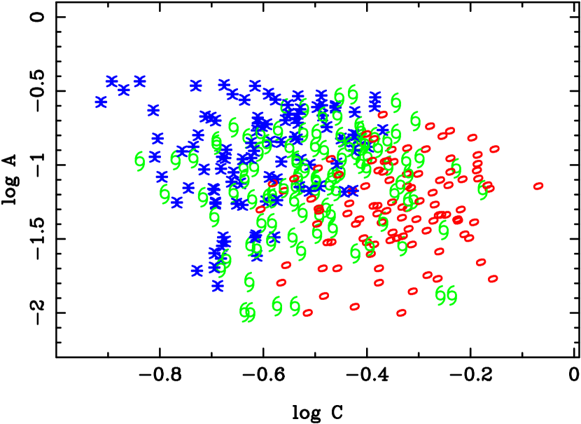
We employ the same procedure for selecting spheroids as described in Menanteau, Abraham, & Ellis (2001a) and Abraham et al. (1996) based on a combination of visual classification and machine morphological analysis. Stars were initially removed using the SExtractor star class parameter in addition to visual inspection of all objects in the sample. Here, we briefly summarize the strategy taken and refer the reader to these works for a full description of the methodology used. Galaxies in the Tadpole field were morphologically classified using an automated classification based on both the central concentration (C) and asymmetry (A) parameters (A – C) from Abraham et al. (1996), as well as using visual classifications made by one of us (FM). Visual classification have been shown to agree very well with A – C classes in previous studies (Brinchmann et al., 1998; Menanteau et al., 1999). The segregation of early-type systems is particularly robust as their chief diagnostic parameter for discrimination is central concentration. It is worth noting the key advantage in adding A – C to visual classes alone, as they represent objective measurements of the morphological properties of galaxies and can be modeled and easily reproduced in the future if required. In building our final sample of spheroids we used a combined criteria of using both A - C and visual classes, which we believe is a robust approach. In figure 2 we compare the A-C values computed for galaxies keyed to their visual classes in three broad categories: E/S0, spiral and irregular. We selected spheroid galaxies as objects which were visually classified as E, E/S0 and S0 in the Hubble scheme. When there were discrepancies between visual classes and A – C, they were examined in detail, to ensure an unbiased selection. In this fashion we constructed a final catalog containing 116 ACS spheroids, which is $\sim 43\%$ larger than the only other HST existing catalog; the HDFs fields with 79 spheroids.

2.4. Bayesian photometric redshifts

Despite the absence of spectroscopic information for galaxies in the Tadpole field, we enhance the sample with the photometric redshift estimates computed using the Bayesian Photometric Redshift package (BPZ) (Benítez, 2000) included in the Apsis pipeline products. BPZ follows a Bayesian statistical approach to estimate redshifts employing a set of galaxy templates and magnitude-redshift priors. While it is often assumed that several filters are necessary to achieve accurate measurements, the addition of priors can lead to reliable redshifts with only the F475W, F606W and F814W filters. As described in Benítez et al. (2004), when the Bayesian methodology is calibrated with the Northern HDF (HDF-N) spectroscopic sample, it has an excellent behavior at $z<1.5$ , without catastrophic outliers and much better performance than maximum likelihood alone. Furthermore, according to Benítez et al. (2004), simulations of the efficiency of the photometric redshifts as a function of magnitude confirmed that for bright objects, $I_{814}\mathbin{\lower 3.0pt\hbox{$\hbox to0.0pt{\raise 5.0pt\hbox{$\char 60\relax$}\hss}\mathchar 29208\relax$}}24$ the tipical uncertainties are $dz/(1+z)\sim 0.1$ , which coincides with the magnitude limit set for our sample where photometric estimates are most reliable. Despite the small estimated errors, we opt to take the safer approach of using the photometric redshift only over the integrated properties of the sample rather than those of individual galaxies.

3. Resolving Spheroids

Understanding the behavior of the point-spread function (PSF) becomes important when studying distant objects at pixel-scales. In the present analysis our main concern is that PSF variations as a function of wavelength may lead to spurious centrally concentrated inhomogeneities arising from some centrally concentrated profiles in some spheroids. To study this effect we made extensive simulations of the effect of the PSF by artificially creating spheroids which were subsequently analyzed using the same method applied to the observed data. These are presented in Appendix A. We conclude that the effect of the PSF will not significantly influence any of the indicators used in our analysis.

Prompted by the findings of spheroids with central blue cores in the HDFs (Menanteau, Abraham, & Ellis, 2001a), the first step in our analysis is to construct $V_{606}-I_{814}$ color maps for all the ellipticals in our sample. This color peculiarity has only been reported for early-types in the HDFs so far, and it is compelling to verify whether it will also be present in other unrelated samples such us the current one. For this, we compute pixel maps, surface brightness, $\mu$ , for all galaxies in all three bands, using the well-known transformation,

\mu={\rm zp}-2.5\log({\rm counts}/{\rm exptime})+5\log({\rm pixelscale})

where zp is the zero-point for a given filter in the Vega system from Table 2, the pixelscale is 0.05 arc/pixel and counts is the number of electrons in each pixel. Subsequently, color maps were computed, selecting only contiguous pixels above a surface brightness threshold of $\mu_{606}\leq 25$ mag/arc sec². We note that we use this surface brightness limit only in the computation of $\delta(V-I)$ in section 4.1 in order to maintain consistency when comparing with previous observations. However in section 4.2 we will discusss a more robust method for selecting and measuring the light of spheroids.

3.1. Old ellipticals vs Blue ellipticals

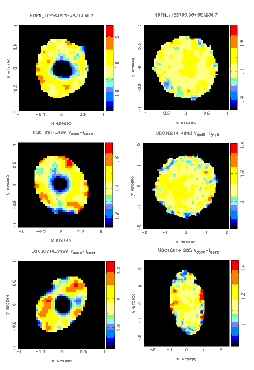
Our first objective is finding a population of spheroids with blue cores and inhomogeneous internal colors in the current ACS sample mirroring those found in the HDFs. After an initial inspection, we conclude that in most cases spheroids show fairly smooth and homogeneous $V_{606}-I_{814}$ color maps, but the existence of a subsample with perturbed internal colors is quite evident. We report a fraction of spheroids with blue cores comparable to the HDFs in our ACS sample, with similar sizes and strength in their color differences. It is important to remark that this is the first sample, apart from the HDFs in which resolved studies of distant galaxies are possible. To illustrate the similarities in our findings, in Fig. 3, we show examples of spheroids with normal and peculiar internal color properties in the HDF-N and the present sample of ACS spheroids. The similarities in the form of the blue nucleated ones in both samples are quite evident.

4. Methodology and analysis

After considering the color maps of spheroids, we want to investigate how the internal colors of field ellipticals vary as a function of redshift and quantify the fraction that departs from a passive evolving population. Although we can identify a distinctive population of spheroids with blue cores and color inhomogeneities from visual inspections alone, we wish to develop a method for quantifying its strength in an objective way. A standard tool for this purpose is to model their color properties using stellar synthesis population models (Abraham et al., 1999; Menanteau et al., 2001b). Unfortunately, these predictions are quite sensitive to the galaxy redshift of observation and our present sample only encompass photometric estimates, making this approach toward characterizing individual galaxies somewhat uncertain. Instead we chose to explore a model-free approach and focus on the integrated properties, which in our view represent a safer way to evaluate the trend of the population. For this purpose we revisit the internal color dispersion estimator from Menanteau, Abraham, & Ellis (2001a) and devise a new measurement based on the slope of the color gradients of a galaxy that we will show is more sensitive to the presence of central blue spots.

4.1. The internal color dispersion $\delta(V-I)$

The idea of studying the internal colors of an individual galaxy can be considered as a generalization of the use of the color-magnitude relation in the study of the history of elliptical galaxies in clusters (Bower, Lucey, & Ellis, 1992), where the photometric dispersion is employed as a powerful mechanism to determine variations in their star formation history. The first quantity that we present is the signal-to-noise weighted scatter in the internal $V_{606}-I_{814}$ colors of a galaxy, $\delta(V-I)$ , as defined in Menanteau, Abraham, & Ellis (2001a). This measurement has proven a good tracer of peculiarities in spheroid colors at pixel scales in the sense that objects with low values of $\delta(V-I)$ have very uniform and normal color maps, while those with higher values do present disturbed internal colors and in many cases blue cores.

A key motivation for re-visiting this estimator is that it has already been applied and calibrated with a similarly selected sample of galaxies in the HDFs, where it proved to be a good discriminant of objects with blue cores vs ellipticals with normal colors. This feature enable us to make direct comparison between the HDFs sample $\delta(V-I)$ measurements and the current one. In addition, it is a model independent method for studying differences in the star-formation histories of galaxies, making it free of assumptions regarding the epoch of formation in ellipticals.

In our estimates of $\delta(V-I)$ , we follow the same procedure used in the HDFs, and we also chose to concentrate only on the $V_{606}$ and $I_{814}$ bands for computing color dispersions, as the resulting $V_{606}-I_{814}$ color contains significantly smaller observational errors than $g_{450}-V_{606}$ , specially for systems dominated by old stellar populations (see Menanteau, Abraham, & Ellis, 2001a, for details). However, it is important to note that strong variations in the internal colors are also present when looking at the the $g_{450}-V_{606}$ colors. We select all contiguous pixels within a surface brightness limit of $<25$ mag/arcsec² in $V_{606}$ , to isolate the galaxy from the background sky and maximize the S/N ratio per pixel associated. Using only the pixels within this limit, $\delta(V-I)$ is computed from the weighted signal-to-noise distribution of $V_{606}-I_{814}$ colors for individual pixels, which in turn identifies the internal homogeneity of a galaxy, using the following recipe:

\delta(V-I)\propto\frac{\sum(x_{i}-\bar{x})^{2}S(x_{i}){\rm{SNR}}(x_{i})}{\sum S(x_{i}){\rm{SNR}}(x_{i})}

(1)

\bar{x}=\frac{\sum x_{i}S(x_{i}){\rm{SNR}}(x_{i})}{\sum S(x_{i}){\rm{SNR}}(x_{i})}

(2)

where $S(x)$ is a selection function for pixels with signal/noise above a certain threshold such that $S(x)=1$ for pixels above and $S(x)=0$ for pixel below the threshold. $SNR(x_{i})$ is the signal-to-noise ratio for a given pixel color $x_{i}$ . The selection function $S(x)$ and the weighting according to $SNR(x)$ address biases arising from noise variations at pixel-scales by rejecting low signal pixels and weighting the pixels’ contribution proportionally to their signal.

4.2. The mean $(V_{606}-I_{814})(r)$ slope of the galaxy

In addition to the color dispersion we wish to develop an alternative quantity to isolate spheroids with non-homogeneous internal colors. This should be suited to measure the strength of the blue cores and not prone to dispersions arising from particularly reddened core. For this we concentrate on a method that quantifies the variation in the color as a function of the galaxy radius. Given that in most of the cases, color peculiarities manifest themselves via the presence of blue cores, a clear pattern of this effect is the display of inverted (i.e. positive sign) color gradient, as opposed to “normal” passively evolving ellipticals which either show flat or slightly negative color gradients, as expected from metal enriched cores.

We focus on the $V_{606}-I_{814}$ colors to compute color gradients as a function of the radius $r$ , as these represent the bands where the signal-to-noise is higher and can be more directly related to $\delta(V-I)$ . In the extraction of the color gradients, initially we measure the centroid and second order moments ( $\overline{x^{2}}$ , $\overline{y^{2}}$ , $\overline{xy}$ ) of the galaxy utilizing the $I_{814}$ band, from which we determine the ellipticity parameters of the objects ( $a,b,\theta$ ). It is worth noting that we keep the same elongation ratio $e=a/b$ up to the isophotal limit to which the color gradient is computed. Next, using concentric ellipses, we calculate the $V_{606}-I_{814}(r_{i})$ gradients as the median color in the shell between $r_{i-1}$ and $r_{i+1}$ . To gauge the slope of the color gradient, we fit a fourth order polynomial function to the observed $(V_{606}-I_{814})(r)$ , up to a certain maximum radius $r_{max}$ , from where we measure the slope by simply obtaining the first derivative of the fitted polynomial function. In order to consistenly measure the slope of galaxies over similar physical areas on spheroids and at different redshifts, we compute the slope up to a radius $r_{max}$ following a similar aproach to the one described by Papovich et al. (2003) and Conselice et al. (2000). This consists of choosing the aperture radius $r_{max}$ of the galaxy as $r_{max}=1.5\times r_{p}$ with $(\eta=0.2)$ where $r_{p}$ is the Petrosian (1976) radius and $\eta(r)$ is defined as:

\eta(r)=I(r)/\langle I(r)\rangle

(3)

where $I(r)$ is the surface brightness of the galaxy in an annulus of radius $r$ and $\langle I(r)\rangle$ is its mean value up to the same radius. The Petrosian radius depends only on the galaxy surface brightness and it is independent of the redshift of observation. Formally, the mean $(V_{606}-I_{814})(r)$ slope of the galaxy can be expressed as:

\overline{slope}=\frac{\sum\frac{d}{dr}(V-I)(r)|_{r_{i}}\cdot\Delta r_{i}}{\sum\Delta r_{i}}

(4)

where the derivative is taken over the fitted function, $\Delta r_{i}$ is the size of the concentric shells and $r$ is measured in kpc. We repeat this procedure to all the galaxies in our sample. In Section 5 we will investigate how it performs compared with $\delta(V-I)$ and present examples.

4.3. Comparing the indicators

An important objective of our analysis, is to carry out direct comparisons of the internal color dispersions between the present ACS sample and those observed in the HDFs. For this purpose, we will include in our study the morphologically selected catalog of spheroids in HDF-N from Menanteau et al. (2001a). The HDF-N sample was constructed using the same selection limits and morphological classification, ensuring a robust comparison between samples. We decide to include only the Northern HDF as this contains the largest number of spectroscopic redshifts, making possible an investigation of how the internal color dispersions vary as a function of redshift as opposed to the photometric estimates in ACS spheroids. After computing $\delta(V-I)$ and the mean slope for all galaxies in the ACS and HDF-N samples we examine how they perform against each other and subsequently compare with HDF-N spheroids.

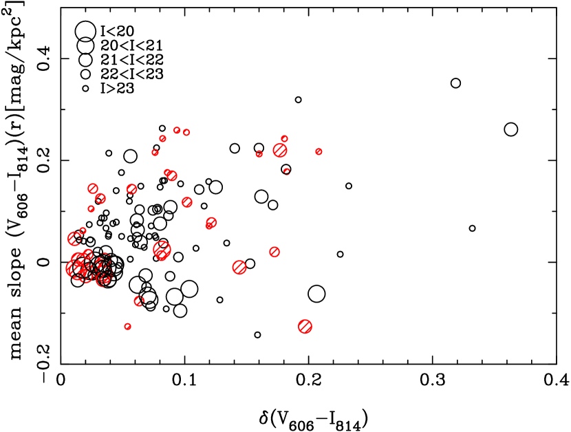
Figure 4 shows the values of $\delta(V-I)$ versus the mean slope $(V_{606}-I_{814})(r)$ for all spheroids in the Tadpole field. We can observe a clear correlation between both statistics for the larger part of the sample: galaxies with high positive mean slopes (indicative of blue cores) also show high values of $\delta(V-I)$ (i.e. high internal color dispersions). Although the inverse relation is true for most galaxies (i.e high color dispersion values ( $\delta(V-I)$ $\mathbin{\lower 3.0pt\hbox{$\hbox to0.0pt{\raise 5.0pt\hbox{$\char 62\relax$}\hss}\mathchar 29208\relax$}}0.06$ ) also have high positive slopes) we see in Fig. 4 that several high $\delta(V-I)$ galaxies have flat or even negative slopes in some cases. This results as galaxies with metal enriched cores tend to have redder centers, making their mean slopes slightly negative or flat, while keeping higher than normal values of $\delta(V-I)$ . From Fig. 4, we wish to highlight that the mean slope $(V_{606}-I_{814})(r)$ is a more robust statistic for tracing blue cores as spheroids with positive slopes and hence blue cores exhibit high internal color dispersion. Also in Fig. 4 we present the values computed for the HDF-N spheroids. It is reassuring that ellipticals populate the same region in the $\delta(V-I)$ —median slope space for both samples. After individually inspecting the objects with high $\delta(V-I)$ values but low or negative slopes, we confirm that these correspond to objects with reddened cores. We conclude that although both statistics succeed in tracing the observed color variations, the mean slope is a more robust statistic for tracing blue light in spheroids and is not prone to color differences arising from color gradients normally accounted for in passively evolved ellipticals.

5. Results

Establishing the existence of a population of field spheroids with marked color dispersions, resembling those exhibited by HDFs spheroids is a major objective of this paper. From the constructed color maps alone we can conclude that this is a property shared by field spheroids at intermediate redshifts regardless of the sample in study. The presence of strong variations in the internal color distributions suggests episodes of recent start-formation activity. However, detailed measurements regarding the intensity and timescales involved requires precise spectroscopic information, not available for the sample in our study. Instead, we opt to determine in a model-independent way the proportion of active systems as a function of redshift and based on this information, make educated guesses regarding the evolution of early-type galaxies.

Initially, we wish to investigate the behavior of $\delta(V-I)$ as a function of redshift. For this, in figure 5 we display the computed values of $\delta(V-I)$ as a function of their photometric estimations for the Tadpole field (open circles) and spectroscopic redshifts for the HDF-N (filled triangles). Error bars represent $1\sigma$ estimates obtained using the bootstrap resampling technique introduced by Efron & Tibshirani (1986). From figure 5 we observe how the fraction of spheroids with high $\delta(V-I)$ values slightly increases as a function of redshift in the same way as reported for HDF-N spheroids. We make a quantitative measurement and focus on the fraction of systems with high $\delta(V-I)$ values compared to low ones as this measurement is not prone to selection effects due to the redshift distribution of spheroids in our sample. We separate the sample into two redshift bins, such as $0<z_{bin1}\leq 0.6$ and $0.6<z_{bin2}\leq 1.2$ and calculate the fraction of spheroids with $\delta(V-I)>0.09$ to the total number. We report an increase from 28% in $z_{bin1}$ to 39% in $z_{bin2}$ . However, we point out that this might also be consistent with no increase given the relatively small number of objects involved.

It is reassuring to confirm that both samples show a very similar trend in the observed spread as well as its increase with redshift. Assuming that in most cases high values of $\delta(V-I)$ are associated with recent star formation activity within the galaxy, the rise of $\delta(V-I)$ with redshift indicates a clear trend in this sense. For the HDFs, Menanteau et al. (2001a) have computed simple models that can explain the existence of galaxies with high $\delta(V-I)$ as the result of small additional bursts of star formation activity.

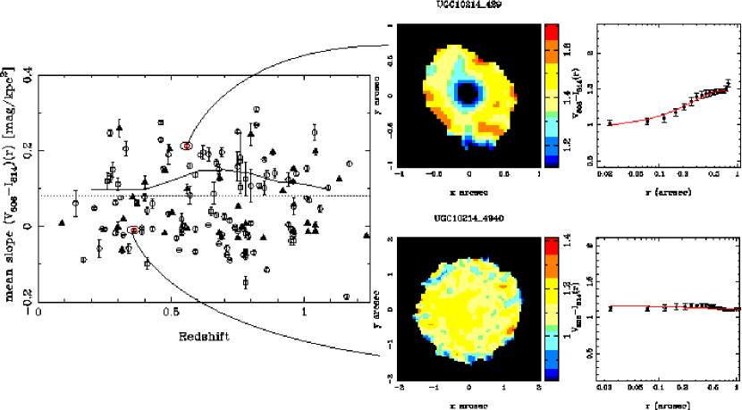
If we assume that strong internal color dispersion are indeed associated with recent star formation, it is interesting to obtain the fraction of evolving systems as a function of redshift. As observed from figure 4, the mean slope $(V_{606}-I_{814})(r)$ is better suited to probe blue cores and internal inhomogeneities than $\delta(V-I)$ , therefore we choose to use this instead of $\delta(V-I)$ for estimating the ratio of spheroids with strong internal color variations to the total number of objects. In figure 6 we show computed values of the mean slope $(V_{606}-I_{814})(r)$ as a function of redshift for both the Tadpole field and the HDF-N sample, using the same symbols as in figure 5. For completeness we also display the values for the HDF-N, as this allows to make consistency checks for variations that could arise between samples, in part due to the use of photometric redshifts. Error bars show $1\sigma$ computations calculated by carrying out Monte Carlo simulations over the data. To illustrate how the mean slope is used in probing galaxies with blue cores, in figure 6 we also show two galaxies of contrasting internal colors and the very distinctive values of the mean slope they have. It is interesting to note from this figure how galaxies tend to populate rather uniformly the redshift space.

5.1. The mean slope $(V_{606}-I_{814})(r)$ redshift dependence

In order to reliably make use of the mean slope $(V_{606}-I_{814})(r)$ in tracing blue light in spheroids, we need to investigate its variation as a function of redshift introduced from measuring the mean slope using the $V_{606}$ and $I_{814}$ filters. We attempt to reproduce through simulations the observed spatially resolved color properties of spheroids with blue nuclei. Our key assumption when modeling these spheroids is that at intermediate redshifts they can be described using a two component model: a young stellar central component (responsible for the blue light) superimposed on an old system. We modeled the integrated $V_{606}-I_{814}$ colors of both stellar component using spectral energy distributions (SED) from the Bruzual & Charlot (1996) (BC96) library. For the old stellar component we chose an SED corresponding to exponentially declining star formation ( $e$ -folding time $1$ Gyr) at age $12$ Gyr, which resembles the colors of a normal elliptical at $z\sim 0$ . For the central region we employ the SED of a recent star-forming elliptical as observed after $1$ Gyr since its formation. For each component their observed $V_{606}-I_{814}$ colors and apparent magnitudes are computed as as a function of redshift ( $K$ -correction only) assuming a flat universe ( $H_{0}=71$ km s^-1Mpc^-1, $\Omega_{0}=0.27$ , $\Omega_{\Lambda}=0.73$ ).

To emulate the geometrical properties of the modeled galaxies (as those of the blue nucleated spheroid in Fig. 6) we created artificial ellipticals from the two components using a customized version of the IRAF package ARTDATA. We used a fixed physical size of half-light radius $r_{e}=3$ kpc for a de Vaucouleurs profile for the old component. We assume that the blue central component corresponds to only $15\%$ of the total stellar mass of the galaxy $M=3\times 10^{11}M_{\sun}$ , as this supplies enough blue light to reproduce the observed blue colors, and effective radius of $0.15r_{e}$ .

For the resulting artificial galaxies we compute the mean slope $(V_{606}-I_{814})(r)$ between $0.2<z<1.2$ using the same procedure as for the real data. We show the results of the exercise in figure 6. The solid line represents the computed values of the mean slope $(V_{606}-I_{814})(r)$ recovered from the simulations. We observe that for simulated spheroids the mean slope changes little as a function of redshift, with a bump at $z\sim 0.65$ which coincides with the peak in the $\Delta(V_{606}-I_{814})$ colors difference between both components. We conclude that although our filter set is more favorable to trace blue light near $z\sim 0.65$ , the variations as a function of redshift are small enough that this will not significantly affect our results.

5.2. The fraction of active systems

When computing the active to total galaxies ratio, we need to calibrate the mean slope $(V_{606}-I_{814})(r)$ to differentiate between active versus passively evolved systems. Certainly high values of the mean slope are directly linked to large internal color variations, and for the high mean slope vs. redshift envelope, is where undoubtedly the most striking cases of blue cores arise. On the other hand, galaxies with small values, near zero or negative show no significant color variations. However, defining a limit that separate active vs passive systems is a rather uncertain and imprecise exercise. To assess this problem, we opt for interactively calibrating this limit, by visually inspecting all galaxies and their respective color maps. After extensive inspections, we resolve to chose a constant limit of mean slope $(V_{606}-I_{814})(r)$ $>0.08$ mags $/$ kpc² as a fiducial limit, that produces the cleanest separation (Fig. 6. Using this limit we proceed and compute the fraction of active to total spheroids as a function of redshift for all the ellipticals in the Tadpole field up to $z\sim 1.2$ . In order to avoid possible uncertainties arising from normal Poisson variations and the use of photometric redshifts, we opt for binning out the data using redshift bins of size $\Delta z=0.25$ , wide enough to smooth out major noise variations. In figure 7 we show the fraction of active to total systems as a function of their photometric redshifts. In order to incorporate the error in the measurement of the photometric redshifts, $1\sigma$ error bars in figure 7 were estimated by carrying out Monte Carlo simulations over the distributions. To estimate the uncertainties we recompute the histogram $N$ times ( $N\sim 1000$ ) in which the redshift of observation of the galaxies is modified such as $z_{o}^{\prime}=z_{o}\pm\alpha\delta z$ , in which $\alpha$ is a randomly generated number between $[-1,+1]$ and $\delta z$ is the nominal error estimation of BPZ equal to $\delta z=0.15(1+z)$ .

From figure 7 we report that the fraction of active spheroids is compatible with constant as a function of redshift (within the error bars). It is important to notice that the estimate for the lowest redshift bin, is quite uncertain as indicated by the large error bars, as the Tadpole sample is incomplete for lower redshift galaxies (see Benítez et al., 2004). Regarding the actual amount of the fraction of active spheroidals, we recognize that its absolute value is rather dependent in the limit used for selection. However, for the current limit adopted, this number mostly fluctuates around $30\%-40\%$ in good agreement with the values obtained for the HDF-N for Kodama et al. (1999) and Menanteau et al. (2001a). It is also worth noting that from tests performed on the sample, the shape of fraction distribution remains largely unchanged when adopting a different limit.

It is appealing to analyze our estimate of the number of active spheroids in the context of their evolutionary history using the simple methodology introduced in this paper. The relatively constant to small rise in the fraction of active systems is suggestive of the presence of a population of active spheroids, continuous at least up to $z\sim 1$ . This can also lead to the interpretation that spheroids are being constantly assembled since $z\sim 1$ . At the same time, the presence of spheroids with homogeneous colors and smooth color gradients is clear evidence of the presence of a relatively dominant population of normal evolved spheroids at all redshifts.

It is possible to ask then, what type of objects are the blue spheroids that we detect? And, what would be their low redshift counterparts? A possible explanation, might be that we are seeing these galaxies as they enter into the E/S0 class, possibly within the first Gyr, since their last star-formation activity. From the modeling of stellar synthesis populations (Menanteau et al., 2001a, b), it is believed that the existence of such populations is not long-lasting. We might be seeing the predecessors or proto-ellipticals, in the last period of star-formation before becoming normal ellipticals as we know them at low redshifts and in clusters of galaxies.

6. Conclusions

In this paper, we have used newly available data from the Advanced Camera for Surveys to study the internal color properties of sample of 116 morphologically selected spheroids. This represents the first deep dataset of spheroids available from the ACS, and we used it to investigate its superb ability to resolve distant galaxies.

Using an independent sample of ACS spheroids we have confirmed the presence of a population of spheroids with color inhomogeneities similar to those found in the HDFs. Using a model independent approach, we have introduced a new statistic, the mean slope $(V_{606}-I_{814})(r)$ which probes successfully the presence of blue cores and internal color inhomogeneities in spheroids. We compare our measurements with the HDF North with consistent results. Assuming that strong variations in the internal color dispersion of spheroids are linked to recent episodes of star formation, we use the mean slope to separate active and passively evolved systems as a function of redshift, and based on this, we estimate the fraction of active systems versus redshift. We found that within the uncertainties of our measurements, the fraction of active galaxies can be described as constant, with a trend to grow with redshift, with nominal values between $\sim 30\%-40\%$ of the sample, consistent with previous results. We take this as evidence for the continuous formation of spheroids since $z\sim 1$ , while the data also shows the presence of a population of old passively evolved ellipticals at all redshifts.

An important part of the challenge that lies ahead is try to understand the significance of the blue spheroids and whether or not these represent the early stages of what we expect to be an elliptical as defined at $z\sim 0$ . Additionally, alternative theories of galaxy formation need to be explored which can explain at the same time the presence of passive evolving systems and recent star-forming spheroids. It also remains to be learned what are the detailed internal properties of ellipticals in clusters are from upcoming ACS observations at $z\sim 1$ (Postman et al. 2004).

ACS was developed under NASA contract NAS 5-32864, and this research is supported by NASA grant NAG5-7697. We would like to thank the anonymous referee for his/her comments and suggestions which improved the paper.

References

Abraham et al. (1999) Abraham, R. G., Ellis, R. S., Fabian, A. C., Tanvir, N. R., & Glazebrook, K. 1999, MNRAS, 303, 641
Abraham et al. (1996) Abraham, R. G., Tanvir, N. R., Santiago, B. X., Ellis, R. S., Glazebrook, K., & van den Bergh, S. 1996, MNRAS, 279, L47
Barger et al. (1999) Barger, A. J., Cowie, L. L., Trentham, N., Fulton, E., Hu, E. M., Songaila, A., & Hall, D. 1999, AJ, 117, 102
Baugh et al. (1996) Baugh, C. M., Cole, S., & Frenk, C. S. 1996, MNRAS, 283, 1361
Bell et al. (2004) Bell, E. F., McIntosh, D. H., Barden, M., Wolf, C., Caldwell, J. A. R., Rix, H., Beckwith, S. V. W., Borch, A., Häussler, B., Jahnke, K., Jogee, S., Meisenheimer, K., Peng, C., Sanchez, S. F., Somerville, R. S., & Wisotzki, L. 2004, ApJ, 600, L11
Benítez (2000) Benítez, N. 2000, ApJ, 536, 571
Benítez et al. (2004) Benítez, N., Ford, H., Bouwens, R., Menanteau, F., Blakeslee, J., Gronwall, C., Illingworth, G., Meurer, G., Broadhurst, T. J., Clampin, M., Franx, M., Hartig, G. F., Magee, D., Sirianni, M., Ardila, D. R., Bartko, F., Brown, R. A., Burrows, C. J., Cheng, E. S., Cross, N. J. G., Feldman, P. D., Golimowski, D. A., Infante, L., Kimble, R. A., Krist, J. E., Lesser, M. P., Levay, Z., Martel, A. R., Miley, G. K., Postman, M., Rosati, P., Sparks, W. B., Tran, H. D., Tsvetanov, Z. I., White, R. L., & Zheng, W. 2004, ApJS, 150, 1
Benson et al. (2002) Benson, A. J., Ellis, R. S., & Menanteau, F. 2002, MNRAS, 336, 564
Bertin & Arnouts (1996) Bertin, E. & Arnouts, S. 1996, Astronomy and Astrophysics Supplement Series, 117, 393
Blakeslee et al. (2003) Blakeslee, J. P., Anderson, K. R., Meurer, G. R., Benítez, N., & Magee, D. 2003, in Astronomical Data Analysis Software and Systems XII ASP Conference Series, Vol. 295, 2003 H. E. Payne, R. I. Jedrzejewski, and R. N. Hook, eds., p.257, 257–+
Bower et al. (1992) Bower, R. G., Lucey, J. R., & Ellis, R. S. 1992, MNRAS, 254, 601+
Brinchmann et al. (1998) Brinchmann, J., Abraham, R., Schade, D., Tresse, L., Ellis, R. S., Lilly, S., Le Fevre, O., Glazebrook, K., Hammer, F., Colless, M., Crampton, D., & Broadhurst, T. 1998, ApJ, 499, 112
Conselice et al. (2000) Conselice, C. J., Bershady, M. A., & Jangren, A. 2000, ApJ, 529, 886
Djorgovski & Davis (1987) Djorgovski, S. & Davis, M. 1987, ApJ, 313, 59
Dressler et al. (1987) Dressler, A., Faber, S. M., Burstein, D., Davies, R. L., Lynden-Bell, D., Terlevich, R. J., & Wegner, G. 1987, ApJ, 313, L37
Efron & Tibshirani (1986) Efron, B. & Tibshirani, R. 1986, Statistical Science, 1, 1
Eggen et al. (1962) Eggen, O. J., Lynden-Bell, D., & Sandage, A. R. 1962, ApJ, 136, 748
Ellis et al. (1997) Ellis, R. S., Smail, I., Dressler, A., Couch, W. J., Oemler, A., J., Butcher, H., & Sharples, R. M. 1997, ApJ, 483, 582
Ford et al. (2002) Ford, H., Clampin, M., Hartig, G., Illingworth, G., Sirianni, M., Martel, A., Meurer, G., McCann, W. J., Sullivan, P., Bartko, F., Benitez, N., Blakeslee, J., Bouwens, R., Broadhurst, T., Brown, R., Burrows, Campbell, D., Cheng, E., Feldman, P., Franx, M., Golimowski, D., Gronwall, C., Kimble, R., Krist, J., Lesser, M., Magee, D., Miley, G., Postman, M., Rafal, M., Rosati, P., Sparks, W., Tran, H., Tsvetanov, Z., Volmer, P., White, R., & Woodruff, R. 2002, in Proc. SPIE Vol. 4854, p. 81-94, in Future EUV and UV Visible Space Astrophysics Missions and Instrumentation, J. C. Blades; O.H. Siegmund; Eds., 81–94
Friaça & Terlevich (2001) Friaça, A. C. S. & Terlevich, R. J. 2001, MNRAS, 325, 335
Hack (1999) Hack, W. J. 1999, ”CALACS Operation and Implementation” (STScI:Baltimore), ACS ISR–99–03
Hinkley & Im (2001) Hinkley, S. & Im, M. 2001, ApJ, 560, L41
Jimenez et al. (1998) Jimenez, R., Padoan, P., Matteucci, F., & Heavens, A. F. 1998, MNRAS, 299, 123
Kodama et al. (1999) Kodama, T., Bower, R. G., & Bell, E. F. 1999, MNRAS, 306, 561
Krist (2003) Krist, J. 2003, ACS ISR 2003-06, STScI:Baltimore
Menanteau et al. (2001a) Menanteau, F., Abraham, R. G., & Ellis, R. S. 2001a, MNRAS, 322, 1
Menanteau et al. (1999) Menanteau, F., Ellis, R. S., Abraham, R. G., Barger, A. J., & Cowie, L. L. 1999, MNRAS, 309, 208
Menanteau et al. (2001b) Menanteau, F., Jimenez, R., & Matteucci, F. 2001b, ApJ, 562, L23
Papovich et al. (2003) Papovich, C., Giavalisco, M., Dickinson, M., Conselice, C. J., & Ferguson, H. C. 2003, ApJ, 598, 827
Peebles (2002) Peebles, P. J. E. 2002, in ASP Conf. Ser. 283: A New Era in Cosmology, ed. N. Metcalfe & T. Shanks
Petrosian (1976) Petrosian, V. 1976, ApJ, 209, L1
Sandage & Visvanathan (1978) Sandage, A. & Visvanathan, N. 1978, ApJ, 225, 742
Sirianni et al. (2004) Sirianni, M., Ford, H. C., Illingworth, G. D., Clampin, M., Hartig, G., Becker, R. H., White, R. L., Bartko, F., Benítez, N., Blakeslee, J. P., Bouwens, R., Broadhurst, T. J., Brown, R., Burrows, C., Cheng, E., Cross, N., Feldman, P. D., Franx, M., Golimowski, D. A., Gronwall, C., Infante, L., Kimble, R. A., Krist, J., Lesser, M., Magee, D., Martel, A. R., McCann, W. J., Meurer, G. R., Miley, G., Postman, M., Rosati, P., Sparks, W. B., & Tsvetanov, Z. 2004, in preparation
Tamura et al. (2000) Tamura, N., Kobayashi, C., Arimoto, N., Kodama, T., & Ohta, K. 2000, AJ, 119, 2134
Trager et al. (2000) Trager, S. C., Faber, S. M., Worthey, G., & González, J. J. 2000, AJ, 120, 165
Tran et al. (2003) Tran, H. D., Sirianni, M., Ford, H. C., Illingworth, G. D., Clampin, M., Hartig, G., Becker, R. H., White, R. L., Bartko, F., Benítez, N., Blakeslee, J. P., Bouwens, R., Broadhurst, T. J., Brown, R., Burrows, C., Cheng, E., Cross, N., Feldman, P. D., Franx, M., Golimowski, D. A., Gronwall, C., Infante, L., Kimble, R. A., Krist, J., Lesser, M., Magee, D., Martel, A. R., McCann, W. J., Meurer, G. R., Miley, G., Postman, M., Rosati, P., Sparks, W. B., & Tsvetanov, Z. 2003, ApJ, 585, 750
Treu & Stiavelli (1999) Treu, T. & Stiavelli, M. 1999, ApJ, 524, L27
Treu et al. (1999) Treu, T., Stiavelli, M., Casertano, S., Møller, P., & Bertin, G. 1999, MNRAS, 308, 1037
van Dokkum & Franx (1996) van Dokkum, P. G. & Franx, M. 1996, MNRAS, 281, 985
White & Frenk (1991) White, S. D. M. & Frenk, C. S. 1991, ApJ, 379, 52
White & Rees (1978) White, S. D. M. & Rees, M. J. 1978, MNRAS, 183, 341
Zepf (1997) Zepf, S. E. 1997, Nature, 390, 377

Appendix A The effect of the ACS/WFC point-spread function

It is known that systematic variations present in the HST PSF may influence studies which depend on small aperture photometry or small galaxies with bright cores. Our main concern is the PSF variation as a function of wavelength, which might induce spurious centrally concentrated color inhomogeneities on sharply peaked light profiles. To investigate the bias level introduced by variations of the PSF in our internal color analysis of spheroids, we carried out Monte Carlo simulations following a procedure similar to the one described in Menanteau et al. (2001a). This consists of creating artificial galaxies using the IRAF package ARTDATA resembling the sizes and brightness as of those in our study. These were subsequently analyzed in the same fashion as the observed data. Initially we attempted to create artificial de Vaucouleurs profiles using a combination of averaged observed bright stars in the background of the Tadpole field as PSF. However, it was soon evident that there was a systematic variation in the PSF FWHM as a function of position in the WFC field. In addition, the small number of bright stars in The Tadpole field made the use of stars as real PSFs too challenging. The PSF variation across the WFC field has been extensively documented by Krist (2003). Although the PSF variations in ACS are less than other HST cameras, its does varies over the field, most notably for the WFC (see Fig. 1 in Krist 2003). Therefore, we chose to utilize the synthetic PSFs generated with the Tiny Tim software as it does take into account field variations.

We created a grid of $4\times 4$ PSFs at evenly distributed positions across both WFC chips with Tiny Tim for the $V_{606}$ and $I_{814}$ bands. These were incorporated into ACS mock raw images and later processed through Apsis using the same parameters as for the observed data. These yield a geometrically corrected grid image of synthetic PSFs. In Fig. 8 we show a diagram with the final positions. Using this grid, spheroids were synthesized at each PSF location with de Vaucouleurs profiles using IRAF’s ARTDATA. A set of simulated spheroids were generated for the $V_{606}$ and $I_{814}$ bands trying to mimic as much as possible the observed properties of spheroids. These include a range of half-light radius ( $r_{e}$ ) from $0.1^{\prime\prime}-0.7^{\prime\prime}$ which correspond to a physical length of $\sim 0.75-5.5$ kpc ( $H_{0}=71$ km s^-1Mpc^-1, $\Omega_{0}=0.27$ , $\Omega_{\Lambda}=0.73$ ) and a range of magnitudes consisted with our sample ( $18<I_{814}<24$ ). We processed the synthetic spheroids using the exact same procedure employed for real spheroids and calculated both estimators, $\delta(V-I)$ and the mean slope $(V_{606}-I_{814})(r)$ for the whole sample. To simplify the simulation we compute the mean slope as function of the object apparent size. As the influence of the PSF in the resolved colors is expected to be a strong function of the ’peakiness’ of light distribution of the galaxy, we probe the influence of the PSF on real and simulated galaxies against the central concentration parameter (section 2.3).

The results of this exercise are shown in Figs. 9 and 10, where we plot the values of $\delta(V-I)$ and the mean slope $(V_{606}-I_{814})(r)$ as a function of the central concentration respectively for the 16 PSF pointings. In all 16 positions we also plot the observed data (open squared) to compare with the simulation results. When confronting real and simulated values of $\delta(V-I)$ in Fig. 9 we can see that over the observed range of $C$ for the ACS spheroids (i.e. $0.3\mathbin{\lower 3.0pt\hbox{$\hbox to0.0pt{\raise 5.0pt\hbox{$\char 60\relax$}\hss}\mathchar 29208\relax$}}C\mathbin{\lower 3.0pt\hbox{$\hbox to0.0pt{\raise 5.0pt\hbox{$\char 60\relax$}\hss}\mathchar 29208\relax$}}0.7$ ) the values of $\delta(V-I)$ for the simulated galaxies as significantly lower that those obtained for the observed spheroids. Only for values of $C>0.8$ we enter into the regime in which the PSF can affect the recovered values of $\delta(V-I)$ as the PSF becomes important. However, our spheroids do not lie in this range. We notice some variation depending on the PSF position used, but this effect is too small for the scale of the real values of $\delta(V-I)$ . We also compare the central concentration with the mean slope $(V_{606}-I_{814})(r)$ using the same symbols as of Fig. 9. The simulated galaxies have mostly a uniform distribution of values of mean slope $(V_{606}-I_{814})(r)$ as a function of $C$ , also lower than the observed for the real data. We conclude that the bias level introduce by the variations in the WFC PSF will not seriously affect any of our conclusions.

Appendix B The Catalog of Spheroids in UGC102104

Table 3The catalog of selected spheroids from UGC102104

\tablenote

Complete table available at http://acs.pha.jhu.edu/ $\sim$ felipe/e-prints ID RA(J2000) DEC(J2000) F814W $\delta(V-I)$ mean slope $(V_{606}-I_{814})(r)$ BPZ A C 1041 16:06:16.49 +55:23:44.19 21.877 $0.0621\pm 0.0019$ $-0.0587\pm 0.0012$ 0.23 0.054 0.538 1076 16:06:03.55 +55:24:54.00 22.982 $0.0146\pm 0.0072$ $0.0292\pm 0.0335$ 0.67 0.032 0.392 1103 16:06:09.86 +55:24:28.60 21.767 $0.0393\pm 0.0026$ $0.0485\pm 0.0026$ 0.21 0.043 0.385 1109 16:06:19.18 +55:24:17.63 23.713 $0.1091\pm 0.0285$ $0.1515\pm 0.0350$ 0.47 0.067 0.275 1142 16:06:06.01 +55:24:53.35 23.408 $0.1284\pm 0.0277$ $-0.0982\pm 0.0386$ 0.41 0.047 0.365 1157 16:06:13.95 +55:24:57.49 21.760 $0.0964\pm 0.0086$ $-0.0765\pm 0.0030$ 0.78 0.052 0.466 1200 16:06:04.61 +55:25:58.07 23.408 $0.5834\pm 0.0079$ $-0.2479\pm 0.0304$ 0.85 0.051 0.477 1207 16:06:01.80 +55:26:17.99 20.447 $0.1038\pm 0.0013$ $-0.0751\pm 0.0009$ 0.71 0.081 0.653 1266 16:06:18.02 +55:24:31.97 23.362 $0.0802\pm 0.0219$ $0.1880\pm 0.0419$ 0.61 0.004 0.451 1275 16:06:19.02 +55:24:25.81 22.822 $0.0882\pm 0.0080$ $-0.0050\pm 0.0077$ 0.74 0.041 0.425 1282 16:06:15.43 +55:24:49.85 23.337 $0.0563\pm 0.0151$ $0.1083\pm 0.0159$ 0.83 0.130 0.476 1295 16:06:03.27 +55:24:57.76 20.654 $0.0701\pm 0.0058$ $-0.0658\pm 0.0473$ 0.78 0.090 0.428 1364 16:06:15.43 +55:24:52.52 23.303 $0.0330\pm 0.0469$ $0.1256\pm 0.0582$ 0.78 0.128 0.702 1475 16:06:19.52 +55:24:30.48 23.856 $0.0490\pm 0.0149$ $0.1673\pm 0.0175$ 0.67 0.040 0.379