Limits on the Optical Brightness of the $\epsilon$ Eridani Dust Ring¹

Abstract

The STIS/CCD camera on the Hubble Space Telescope (HST) was used to take deep optical images near the K2V main-sequence star $\epsilon$ Eridani in an attempt to find an optical counterpart of the dust ring previously imaged by sub-mm observations. Upper limits for the optical brightness of the dust ring are determined and discussed in the context of the scattered starlight expected from plausible dust models. We find that, even if the dust is smoothly distributed in symmetrical rings, the optical surface brightness of the dust, as measured with the HST/STIS CCD clear aperture at 55 AU from the star, cannot be brighter than about 25 STMAG/”². This upper limit excludes some solid grain models for the dust ring that can fit the IR and sub-mm data. Magnitudes and positions for $\approx\,$59 discrete objects between 12.5” to 58” from $\epsilon$ Eri are reported. Most if not all of these objects are likely to be background stars and galaxies.

1 Introduction.

A substantial fraction ($\approx 15$%) of main-sequence stars show evidence for excess IR or sub-mm flux due to thermal emission from dust located at distances of 30 AU or more from the stars; i.e., locations comparable to that of the Kuiper Belt in our own Solar System. This was first discovered using IRAS observations (e.g., Aumann et al. 1984; 1985; Gillett & Aumann 1983), and subsequently, observations with the James Clarke Maxwell Telescope’s Submillimeter Common-User Bolometer Array (JCMT/SCUBA) have directly imaged the dust distribution in a few of these systems (Holland et al. 1998), including $\epsilon$ Eri (Greaves et al 1998).

$\epsilon$ Eridani is a K2V main-sequence star at a distance of about 3.2 pc. It is believed to be a relatively young system ($<1$ Gyr; Song et al. 2000; Soderblom & Dappen 1989), with a mass slightly less than our own Sun. From radial velocity measurements, Hatzes et al (2000) have reported evidence for a planet in this system with a semimajor axis of 3.4 AU and $m\sin i=0.86M_{J}$.

The 850$\,\mu$m observations of Greaves et al. show a ring-like structure around $\epsilon$ Eri. The maximum surface brightness of this ring is located at a radius of $\approx\,$17” (55 AU) from the star, with some flux extending out as far as 36” (115 AU). The observed 850$\,\mu$m flux shows the ring to be asymmetrical, with several bright clumps. It has been suggested that structures of this kind can be caused by resonant interactions of dust with planets in or near the ring (Liou & Zook 1999; Ozernoy et al 2000; Quillen & Thorndike 2002).

In an attempt to detect an optical counterpart of this ring we undertook observations with the Hubble Space Telescope’s Space Telescope Imaging Spectrograph (HST/STIS) of $\epsilon$ Eri, using this instrument’s CCD camera, as part of HST GO program 9037 (Mario Livio PI). A full description of the STIS instrument can be found in Kim Quijano et al. (2003).

While this camera can be used with a number of coronagraphic wedges, saturation of the detector by the wings of the stellar PSF near the edges of the wedge would severely limit the exposure time achievable in a single image. Therefore, we instead used the 52”X52” clear CCD aperture and placed the star $\approx 5$” off the edge of the detector. The K0 IV star $\delta$ Eri was also observed as a PSF comparison star.

1.1 Details of Previous Observations

Gillett (1986) reconsidered the IRAS observations of $\epsilon$ Eri and concluded that the intrinsic FWHM of the source flux at 60$\,\mu$m was less than 17” in the IRAS scan direction and less than 11” in the perpendicular direction. If this suggestion is correct, it would imply that the bulk of the IRAS emission comes from a region inside of the ring detected by Greaves et al. (1998). However, both the sub-mm ring and the IRAS size limits suggested by Gillett are significantly smaller than the nominal IRAS 60$\,\mu$m resolution at of about 1’ (Beichman et al., 1985), and therefore Gillett’s conclusions should be treated cautiously.

Greaves et al. observed the system with SCUBA at both 850 and 450$\,\mu$m. The 850 $\,\mu$m observations used a beam of 15” FWHM, and Greaves et al published smoothed versions of the images produced by these observations. The S/N of the 450$\,\mu$m observations is too low to give any useful spatial information (no image was published), but it does supply a useful measure of the total flux.

Schütz et al. (2004) obtained 1200 $\mu$m measurements using a 25” beam, that are consistent with Greave et al.’s measurements. Several previous sub-mm observations (Chini et al. 1990; 1991; Zuckerman & Becklin 1993) at various wavelengths (800 – 1300 $\mu$m) had used single pointings with beam-sizes and background chopping too small to properly measure the structure detected by Greaves et al. (see also Weintraub & Stern 1994). While these observations may provide some useful constraints, they cannot be used as direct measures of the flux and are not further considered here.

We summarize the IRAS, Greaves et al., and Schütz et al. data in Table 1. In this table we adopt Greaves et al’s color corrections, as well as their corrections for the stellar contribution to the total flux, and present only the flux attributed to the dust alone.

At 55 AU, the IRAS and SCUBA data imply grain temperatures of about 30 K – close to the equilibrium black body temperature. The very flat 450$\,\mu$m to 850$\,\mu$m flux ratio ($4.6\pm 2.6$) requires the presence of large grains ($>100\,\mu$m), which can emit efficiently at sub-mm wavelengths. At this distance, the time scale for the orbital decay of 100$\,\mu$m grains due to the Poynting-Robertson effect is about $7\times 10^{8}\,$yr; a time scale which is comparable to the inferred age of the system. This would seem to argue against a substantial population of smaller grains in the outer parts of the system. However, recent works on various debris disk systems (e.g., Wyatt et al. 1999; Li, Lunine, & Bendo 2003) have shown that this kind of interpretation is overly simplistic. The sub-mm emissivity of grains drops rapidly enough with decreasing grain size that a substantial population of smaller grains has little effect on the sub-mm flux ratios, and the collision and fragmentation rate of the large grains required by the sub-mm data is still high enough to replenish the smaller grains faster than the Poynting-Robertson effect can remove them. We will see that the nature and abundance of these smaller grains has dramatic effects on the optical detectability of the dust in the $\epsilon$ Eri system.

2 Description of the Observations

The HST observations in this program were done on January 26, 2002 using six adjacent single-orbit visits (see Table 2). In each visit, after taking an ACQ exposure to determine the position of the targeted star, 15 offset exposures of 109 seconds each were taken using the unfiltered STIS CCD in imaging mode. During these offset exposures the bright star was located about 5” off the detector (near CCD pixel coordinates x=1127, y=514). The first and last orbits were used to observe the PSF of the comparison star, $\delta$ Eri at two different orientations differing by 30^∘. The four intermediate orbits were used to observe the primary target at four different orientations separated by 10^∘ intervals. In each of these latter exposures, the position of the brightest sub-millimeter clump observed by Greaves et al. was imaged on the 1024x1024 pixel detector.

The clear aperture used with the STIS CCD is designated as the ”50CCD” aperture in STIS documentation. It has a field of view of almost 52”$\times$52”, and has a very broad bandpass, with significant throughput from about 2000 Å to 10200 Å. Prior to the installation of ACS, STIS 50CCD observations provided the most sensitive HST mode for deep imaging. We will, for the most part, give our observed STIS magnitudes in STMAG units, where the magnitude is defined as $-2.5\log(F_{\lambda})-21.10$, with $F_{\lambda}$ in ergs$/$s$/$cm²/Å. For STIS 50CCD imaging, the conversion to a magnitude system that uses Vega as the zero point is VEGAMAG(50CCD)$=$STMAG(50CCD)$-0.36$.

In addition, at the beginning of each orbit a very short observation was taken of each star using the STIS CCD with the F25ND3 filter (Table 3).

3 Data Analysis

3.1 Basic Analysis

The standard STIS pipeline software was used to produce bias and dark subtracted and flat fielded images of individual subexposures (flt files). Comparison with median filtered images was done to identify and correct hot pixels that were not handled properly in the standard analysis; about 0.5% of pixels were corrected in this way.

Each of the 15 subexposure flt files was rearranged into five separate files, each containing three adjacent subexposures, and these files were input into the stsdas stis routine ocrreject to produce five separate cosmic ray rejected (crj) files for each of the six visits - 30 crj files in total.

In each of these crj files, the two diffraction spikes from the star ($\epsilon$ Eri or $\delta$ Eri) located 5” off the edge of the detector are the brightest features visible. These were used to register the images. As we are primarily interested in the relative offsets between the images, any small systematic offset from the real location of the star relative to the detector is unimportant. Each of the 30 crj files was then shifted so as to put the intersection of the diffraction spikes at the mean location measured for all visits. The shifts applied were up to $\pm 0.7$ pixels in x and $\pm 0.3$ pixels in y. Because we wanted to distort the high S/N pattern of the PSF as little as possible, we shifted the images using a seven point sinc interpolation function with the iraf imshift routine. The shifted crj files for each visit were then combined by again using the STIS ocrreject routine, producing a single aligned crj file for each visit.

We investigated whether there was any advantage in shifting each individual subexposure, rather than combining them first by groups of three before shifting and coadding, but this does not appear to significantly improve the final coadded image.

3.2 PSF subtraction

Subtraction of the PSF from the wings of the a bright star is very sensitive to small mismatches in the target and PSF star’s spectral energy distribution, as well as to small changes in telescope focus and breathing (i.e., changes in image quality caused by flexure of HST and STIS optical elements). We will use two separate techniques to subtract $\epsilon$ Eri’s PSF. Roll deconvolution techniques use the target as its own PSF star, by taking back-to-back observations at different orientations. Direct subtraction of the $\epsilon$ Eri and $\delta$ Eri observations will also be done. A comparison of different PSF subtraction techniques for STIS Coronagraphic observations was done by Grady et al. (2003), and much of their discussion will also be relevant here.

3.2.1 Roll Deconvolution of $\epsilon$ Eri

The goal of the roll deconvolution is to use images taken at different orientations to separate the real sky image from the PSF of the bright nearby star. This technique eliminates any problem with mismatches in the shape of the PSF due to differences in the spectral energy distributions, but it has the disadvantage that any circularly symmetric features or arc-like structures larger than the change in roll angle will be included with the PSF rather than as part of the sky image. Unfortunately these are exactly the type of structures most likely in a circumstellar debris disk.

To obtain a first approximation to the PSF of $\epsilon$ Eri, we combined the four aligned and coadded $\epsilon$ Eri crj images, rejecting points that were high or low by more than three sigma from the median value for that pixel location by using the iraf imcombine routine with the “ccdclip” algorithm. As the images were not yet rotated to align them on the sky, this clips out real objects as if they were cosmic rays. This trial PSF was then subtracted from each of the original images. These subtracted images were each rotated about the position of $\epsilon$ Eri to align the positions on the sky and then combined by taking a straight average of the values at each pixel, but with locations near the main diffraction spikes or the obstructed edges of the 50CCD aperture masked out of the average. We found that masking out a rather wide strip (about 3.4” in the diagonal direction) around the main diffraction spikes gave the best results.

A number of faint objects are clearly visible in the field of view. A mask was created for each unrotated image that identifies pixels that are affected by real objects on the sky.A final PSF for $\epsilon$ Eri was then made in the same way as the initial PSF image, but with these sky objects masked out before taking the average. The new PSF was then subtracted from the shifted crj images, and the subtracted files were again rotated into alignment and averaged after masking out the diffraction spikes and aperture edges.

To summarize, we masked out the sky objects when averaging the unrotated and unsubtracted images to create the PSF, and then masked out the diffraction spikes and aperture edges when averaging the rotated and PSF-subtracted images to create the image of the sky. In principle this procedure could be iterated to refine the separation between the sky and PSF images, but we will simply use the second version of the sky and PSF images produced by this procedure.

3.2.2 Direct Subtraction of $\epsilon$ and $\delta$ Eri’s PSFs

$\delta$ Eri PSF The procedure used to produce the $\delta$ Eri PSF was similar to that used to produce the $\epsilon$ Eri PSF. It was necessary to mask out a generous region around the brightest background star in each of the two $\delta$ Eri images to avoid introducing obvious artifacts in the subtraction.

Relative Normalization of the Two Stars

Before subtracting the $\delta$ Eri PSF from the observations of $\epsilon$ Eri, it is necessary to know both $r$, the relative normalization of the two PSFs, as well as $b$, the sky background level. The PSF subtracted images will then be calculated as $I=(I_{\epsilon}-b)-r(P_{\delta}-b)$.

To calculate the relative normalization we need to consider the spectral energy distributions (SEDs) of the two stars. We will approximate these SEDs by using the broad-band photometry (Table 4) taken from the Lausanne online database (Mermilliod, Mermilliod, & Hauck 1997). Longward of the $V$ band, the two stars have very similar spectral distributions, but $\epsilon$ Eri is a bit bluer at shorter wavelengths. We supplement this photometry with IUE data for shorter wavelengths to provide a rough spectral energy distribution for each star (Table 5), which is then used with SYNPHOT to predict STIS CCD imaging magnitudes in the 50CCD and F25ND3 filters. The predicted F25ND3 magnitudes are about 8% brighter than observed, but the predicted ratio of the two stars’ F25ND3 count rates matches the observed ratio to within 0.2%. This gives us a fair measure of confidence that the predicted flux ratio for STIS CCD imaging with the unfiltered 50CCD aperture will also be correct.

We have also constructed Tiny Tim (Krist 1993; 1995) models using the above spectral energy distributions as input. Tiny Tim only calculates on-axis PSFs for STIS, and does not calculate the PSF beyond  4.5” radius. The ratio of the Tiny Tim PSFs does show that, when normalized to the same total flux, the slightly bluer $\epsilon$ Eri SED results in a PSF at 4.5” that is about 0.4% lower than that of $\delta$ Eri. Taking the predicted 50CCD ratio of 0.837, and then assuming the same difference between the predicted and observed ratios as was found for the direct F25ND3 images ($0.837-0.845$), would give an expected ratio of 0.839. Extrapolating the radial color difference found in the Tiny Tim models, we estimate an additional correction of about $-0.005$ near 17”, yields an estimated normalization ratio of 0.834. If this ratio is adopted, it is also necessary to assume a mean sky background of $\approx$0.077 e^-/pixel/s if the farthest parts of the two PSFs are to match. This is comparable to the expected sky brightness.

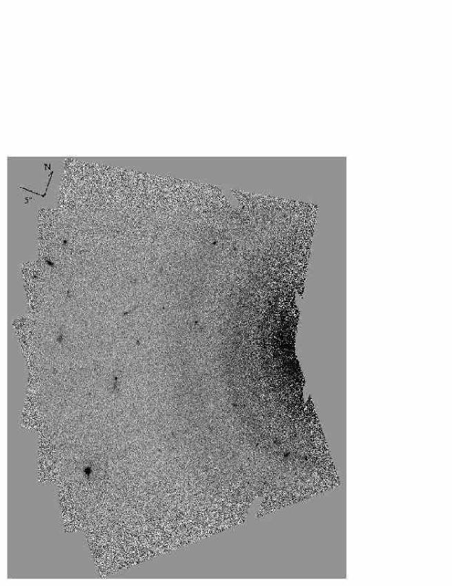
Figure 2: Result of subtracting the two stars’ PSF assuming a normalization factor of 0.834. This normalization leaves a central excess as well as two 5” wide rings with radii of approximately 18” and 28”.

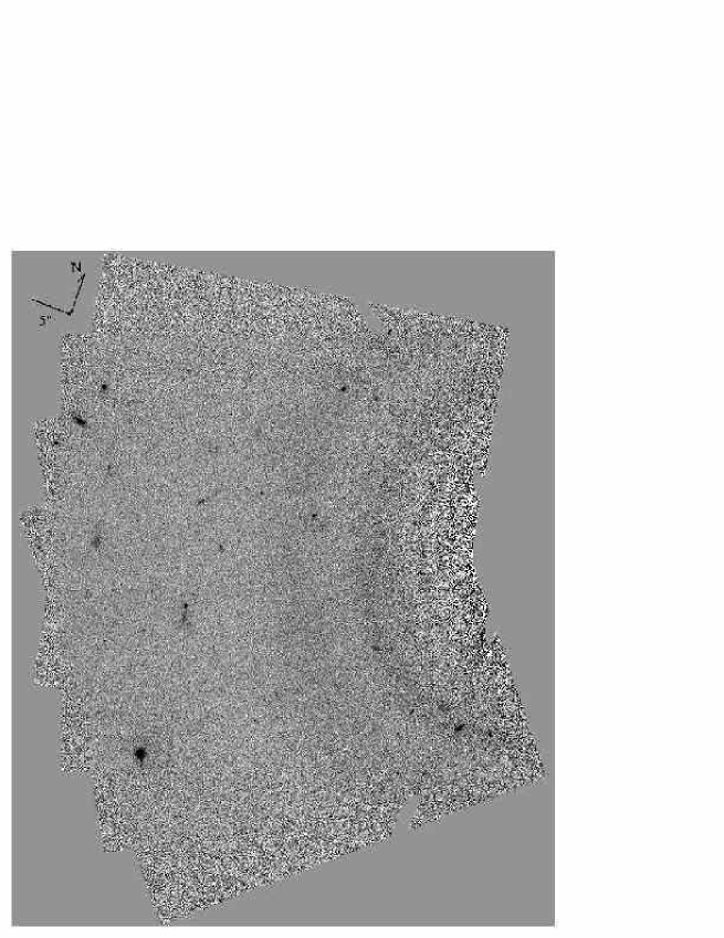
Figure 5: Result of subtracting the two stars’ PSF assuming a normalization factor of 0.842. This normalization minimizes the mismatch in flux close to the star, but the two broad rings remain.

The results of this subtraction are shown in Figure 2. There appears to be substantial excess light near $\epsilon$ Eri, amounting to about 1% of the unsubtracted PSF at the same radius, and a number of concentric rings are visible. To illustrate this diffuse structure we took the difference between the $\epsilon$ and $\delta$ Eri PSFs (with the sky objects removed), and measure the mean surface brightness as a function of radius (Figures 3 and 4). We can minimize the central halo around $\epsilon$ Eri by increasing the normalization constant to about 0.842 (see Fig. 5), but the concentric rings remain, with a mean surface brightness of 25.5 to 25 STMAG/arcsec^-2. If we assume the rings extend all the way around the star, this flatter normalization corresponds to a total integrated STMAG of 17.4 for the rings.

This structure seems suspiciously symmetrical to be consistent with the observed clumpiness in the sub-mm observations, but the radial distribution of the flux, with a broad hump between 15 and 30”, is roughly consistent with the radial dependence of the 850$\,\mu$m flux as shown in Figure 2 of Greaves et al. The rings are broader than PSF subtraction artifacts previously seen in STIS coronagraphic imaging (Grady et al. 2003), however few images expose the far PSF wings this deeply. One example of ACS coronagraphic observations of Arcturus did show that breathing induced changes between visits can lead to a ring in the subtracted image with a radius of 13” and a surface brightness 20.5 mag arcsec^-2 fainter than the star (see figure 5.12 of Pavlovsky et al. 2003). It may be that the rings in our STIS data are a similar artifact. However, we will not completely ignore the possibility that the rings might be real, and will consider whether they could be plausibly modeled by dust in the $\epsilon$ Eri system.

4 Results

4.1 Comparison of the STIS images with the sub-mm emission

4.1.1 Comparison with roll-subtracted images.

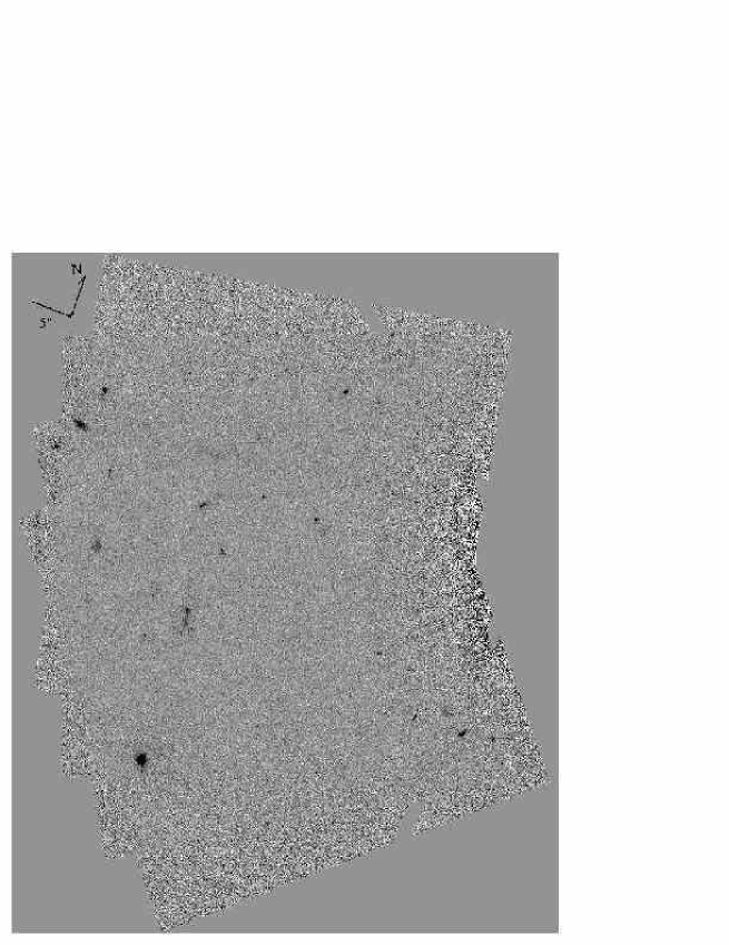
Figure 1: Full mosaiced, roll subtracted image of the targeted field near $\epsilon$ Eri. This, and other images of this field are aligned with the STIS observation o6eo03020, with the +y direction aligned 20 degrees east of north. The compass drawn in the upper left corner of this figure is 5” on a side.

Figure 6 shows the roll subtracted data from part of figure 1, but at two times the scale of that figure and after smoothing with a 5x5 boxcar filter to suppress the small scale noise. Overlaid on this figure is the sub-mm contour map of Greaves et al. (1998), positioned assuming that the sub-mm emission shares the proper motion of $\epsilon$ Eri. The inner contour level of the brightest sub-mm peak is about 5” in diameter.

There are a substantial number of faint objects detected in the region of the sub-mm emission, but the density of such objects is not appreciably greater than elsewhere in the image. There is no apparent correlation between these objects and the sub-mm flux, and most or all of these objects are probably background galaxies or stars. Note that the orbital period for material in the dust ring is about 500 years, and the expected orbital motion is only about 0.2” per year.

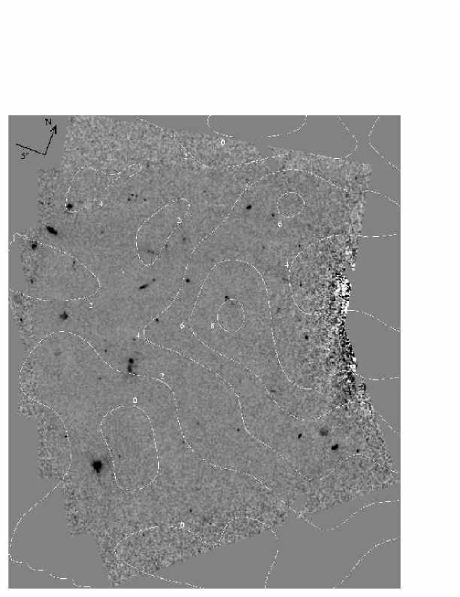
Figure 7: The same as figure 6, but without correcting the sub-mm contours for the proper motion of $\epsilon$ Eri.

Figure 7 shows the same data, but leaves the sub-mm contours at where they were actually observed in 1997-1998; i.e., they are not corrected for the $\approx$4” that $\epsilon$ Eri moved during the intervening years. In this figure, the brightest sub-mm clump is just outside the 2” sub-mm pointing uncertainty of what appears to be a background galaxy with STMAG=24.7 (this brightness includes all the clumps in this extended object).

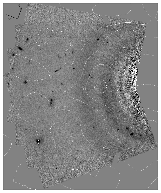
Figure 8: The same as figure 6, except that this time the contours are compared with the sky image made by subtracting the PSF derived from the $\delta$ Eri observations (see Fig 5).

Figure 8 compares the proper motion corrected sub-mm contours with a 5x5 boxcar smoothing of the image that results when subtracting the $\delta$ Eri PSF from the $\epsilon$ Eri data. One of the bright rings is roughly at the location of the sub-mm emission, but there is no correlation with the bright knots.

4.2 Detected Objects Near $\epsilon$ Eri

Nearly sixty distinct objects are visible in the field of view, including about half a dozen within 20” of $\epsilon$ Eri. Most of these objects appear to be slightly extended, and many have complex morphologies. There is no apparent increase in their density at close distances to $\epsilon$ Eri, and most are probably background galaxies. Two relatively bright point sources are visible at distances of 51.5” (STMAG=19.6) and near 54” (STMAG=22.2). A list of detected objects, their locations, and their magnitudes is given in the appendix (Tab. 9). For comparison, we estimate, from the magnitudes and colors given by Chabrier et al. (2000) for models of 1 Gyr old brown dwarfs with dusty atmospheres, that a $0.05M_{\odot}$ brown dwarf in the $\epsilon$ Eri system would have a STIS 50CCD STMAG of about 19, and a $0.03M_{\odot}$ brown dwarf an STMAG of about 27.5.

4.3 Point Source and Surface Brightness Detection Limits

We measured the pixel-to-pixel rms variation in apparently blank regions of the final composite roll-subtracted image as a function of radius from epsilon Eri. The point-to-point rms noise varies smoothly and can be fit as $\sigma\approx 31/r^{3.16}+0.011$ e-/sec, where r is the distance in arc-sec from epsilon Eri. The measured noise is close to that predicted by a simple noise model based on the read noise and the total number of counts in the PSF as a function of radius. Within 30” of the star, the noise in the PSF subtracted image is dominated by the Poisson noise of the star’s PSF wings (although the PSF has been subtracted, its Poisson noise still affects the subtracted image). Since surface brightness of the stellar PSF increases steeply closer to the star, our limiting magnitudes become significantly brighter. At distances greater than 30”, the accumulated read noise dominates the total noise. The measured and predicted noise are listed in Table 7. This noise will be somewhat higher in regions which were not observed at all four orients. Note that a total count rate of 1 e^-/s corresponds to a 50CCD STMAG of 26.405, and that the magnitude of $\epsilon$ Eri in these same units is 4.02.

For extremely red objects, as little as 10% of the total point source counts will fall into the central pixel of 50CCD images. For an unambiguous point source detection, this central pixel should be at least 5$\sigma$ above the rms noise. These assumptions lead to the detectability limits given in the final column of Table 7.

For extended objects, the entire flux should be considered, but a 5 sigma detection will still be required. If noise in different pixels was uncorrelated, then the upper limit for detecting a fixed value of the surface brightness would decrease as the square root of the area. For very large areas, however, any low-spatial frequency noise sources would limit the practically achievable faint limit.

We empirically tested the real faint limit for extended sources by masking out discrete sky objects and then comparing the measured background counts in a number of separate regions at various distances from $\epsilon$ Eri in the roll subtracted image. Taking the standard deviation of the mean fluxes in boxes of a given size at a given distance as the $1\,$sigma error in the background measurement together with the Poisson noise from the potential source, we derive the $5\,\sigma$ detection limits given in Table 8. For boxes $<0.5$”$\times 0.5$”, we found about the variance expected from scaling the point-to-point fluctuations by $1/\sqrt{n_{\rm pix}}$, but for larger areas, the fluctuations were bigger than would be expected from Poisson statistics. For example, when averaging over a $3.5"\times 3.5"$ box at 20”, the measured pixel-to-pixel variance would imply a $5\,\sigma$ detection limit of about 27.2 STMAG/arcsec^-2 – about 1 mag fainter than the directly measured limit. This difference could be due in part to real sources on the sky, but the lack of a clear correlation of these fluctuations with the sub-mm map or distance from the star, requires us to treat such fluctuations as noise.

Note that at 20” from the star, the shift in position from a 10 degree roll change is about 3.5”. Circular or arc-like structures much larger than the roll separation will tend to be washed out in the roll-subtracted image. Unfortunately, long narrow arc-like structures oriented in the tangential direction are precisely the kind of structures that are most likely in circumstellar debris disks. This limits the utility of the roll subtracted image for detecting circumstellar structures much larger than a few arc-seconds in extent.

5 Modeling the dust in the $\epsilon$ Eri system

5.1 The size distribution of dust in circumstellar debris disks.

Collisional fragmentation in a sufficiently dense debris disk will lead to a collisional cascade that generates a wide spectrum of particle sizes. Wyatt et al. (1999), discussed extensively the processes that influence the resulting size distribution. Theoretical arguments predict that, when collisions produce similar fragmentation at all size scales, the cascade leads to a distribution of particle sizes $dn(a)\propto a^{n}da$ (Dohnanyi 1969; Tanaka, Inaba, & Nakazawa 1996), with $n\simeq-3.5$. Such a distribution has most of the mass concentrated in the biggest objects, but with most of the surface area being dominated by particles near the lower end of the size distribution. When the emissivity is constant for all sizes, then the observable characteristics will then be dominated by the smallest particles.

The distribution may, however, be considerably flattened if the orbital evolution of the smaller particles affects them rapidly enough. The lower cutoff to the distribution is set either by the size at which the time scale for Poynting-Robertson driven orbital decay is smaller than the lifetime of these particles against collisional creation, or when the smallest grains can be blown out of the system by radiation pressure.

A small particle broken off a large object in a circular orbit will be on an unbound hyperbolic orbit when the ratio of radiation to gravitational forces $\beta_{\rm rad}>0.5$. We can calculate $\beta_{\rm rad}$ using the same Mie calculations and stellar spectrum used to calculate the dust spectrum (see § 5.2.1).

The time for Poynting-Robertson orbital decay is proportional to the ratio of gravitation to radiative forces on a dust grain. The time scale for Poynting-Robertson drag to change a circular orbit from an radius $r_{1}$ to $r_{2}$ is (Burns, Lamy, & Soter 1979)

$$t_{pr}=400(M_{\odot}/M_{*})(r_{1}^{2}-r_{2}^{2})/\beta_{\rm rad}\rm{\ yr},$$ (1)

where $r_{1}$ and $r_{2}$ are given in AU. For numerical comparisons we will define the time needed for the orbit to decay by 20% of its initial radius as the time scale for Poynting-Robertson drag; this is 36% of the time to decay to zero radius. At a distance of 60 AU from $\epsilon$ Eri, and assuming the age of the system to be about 0.5 – 1 Gyr, the Poynting-Robertson effect would be expected to remove any grains smaller than $\approx$100$\,\mu$m size unless the disk is dense enough that the small particles are still being generated in collisions.

For the smallest particles in a debris disk, Wyatt et al. (1999) estimated that the collisional time scale is of order $t_{\rm{orb}}/4\pi\tau$, where $t_{\rm{orb}}$ is the orbital period and $\tau$ is the effective face on optical depth (i.e., the geometric filling factor). They also estimated that particles will only be destroyed in collisions with particles larger than a factor of $0.03\left[(M_{\odot}/M_{*})(r/r_{\oplus})\right]^{1/3}$ times their own size (about 12% at 60 AU from $\epsilon$ Eri), so we will define $\tau_{d}$ to be a function of the particle size by integrating only over the appropriate size range, and the time scale in years for fragmenting collisions is then:

$$t_{d}={\sqrt{(r/r_{\oplus})^{3}(M_{\odot}/M_{*})}\over{4\pi\tau_{d}}}\simeq 3.7\times 10^{5}\left[\left({r\over 60r_{\oplus}}\right)^{3/2}\left({M_{*}\over M_{\odot}}\right)^{-1/2}\left({\tau_{d}\over 10^{-4}}\right)^{-1}\right]\,yr.$$ (2)

For a dust model to be self consistent, this time scale should be shorter than $t_{pr}$ for even the smallest particles in the model. We will see below that this condition is easily satisfied for the debris disk around $\epsilon$ Eri.

5.2 Calculation of dust models.

5.2.1 Calculating the spectrum of optically thin circumstellar dust

Given an assumed grain composition and the associated wavelength dependent optical constants, we performed standard Mie theory calculations for spherical particles covering a wide range of radii $a$ using the code of Wiscombe (1979; 1980). This gives, among other quantities, the standard scattering and absorption coefficients $Q_{\lambda,sca}$ and $Q_{\lambda,abs}$. (The emission coefficient at each wavelength $Q_{\lambda,em}=Q_{\lambda,abs}).$

For the dust calculations we adopt the flux from a standard solar abundance Kurucz model atmosphere with $T_{\rm eff}=5180K$ and $\log g$=4.75, normalized to a total stellar luminosity of 0.35$\,L_{\odot}$. The dust is assumed to be optically thin, and the temperature of each dust grain can be determined by the equilibrium between absorbed stellar radiation and thermal emission. Once the temperature of the grain is determined, then we can calculate the total light from a dust grain at each wavelength as the sum of the scattered starlight and the thermal emission. We will assume that the dust grain is small enough that the thermal emission is isotropic. The scattered light, however, will be highly anisotropic. The angular phase function $f(\theta)$ for this scattering can be easily derived from the Mie calculation, and we normalize this function so that $f(\theta)=1$ for isotropic scattering. Then, when viewed at a scattering angle $\theta$, the apparent flux of the dust grain will be

$$F_{\lambda,g}=\pi a^{2}Q_{\lambda,sca}F_{\lambda,d}f(\theta)+4\pi a^{2}\pi B_{\lambda}(T)Q_{\lambda,em}$$ (3)

This result will be used below to calculate the expected optical spectrum for a given dust distribution.

5.2.2 Dust composition and porosity

The observable dust particles in circumstellar debris disks are presumed to be collisionally produced fragments of larger objects resembling those in the solar system’s Kuiper belt. These larger objects were probably formed as very porous agglomerations of interstellar grains early in the history of the system.

For the composition and optical properties of these grains we will adopt the model of interstellar and circumstellar dust developed by Li & Greenberg (1997; 1998), which assumes that the dust grains are a mixture of silicates, organic refractories, and voids, with some fraction of the voids possibly filled in by water ice. The Bruggemann mixing rule (Krügel 2003) is used to calculate the effective optical constants for the resulting mixtures from the optical constants of organic refractories and amorphous silicates given by Li & Greenberg (1997), and that of vacuum.

Wyatt & Dent (2002) were able to fit the sub-mm and IRAS data for the debris ring around the A3V star Fomalhaut by assuming solid (non-porous) grains consisting of 1/3 silicate and 2/3 organic refractory material by volume, and a grain size distribution close to the theoretically expected $n^{-3.5}$ that extended down to the radiation blowout limit for that star. While they could not completely exclude models with some degree of porosity in the grains, they argued that the collisional fragmentation should have resulted in significant compaction of the grains despite the high porosity expected in the primordial parent bodies.

In contrast, Li & Greenberg (1997; 1998), and Li & Lunine (2003ab) favor models for the debris disks around HD 141569A, $\beta$ Pictoris, and HR 4796A that assume highly porous grains, with vacuum fractions, $P\approx 0.7$ to 0.9. In some cases these require a dust size distribution close to $dn\propto a^{-3}da$, significantly flatter than the theoretically expected $dn\propto a^{-3.5}da$.

Li, Lunine, & Bendo (2003) have recently fit such a model to the available data for $\epsilon$ Eri. They find that a model assuming highly porous particles, and a rather flat size distribution, can provide an excellent fit to both the IRAS and sub-mm data. They assumed that the same dust-size distribution function applies at all distances from the star, and only varied the total number density of grains as a function of radius to match the distribution of the observed 850$\,\mu$m flux. It is not clear whether or not this is realistic. Moro-Martín’s & Malhotra’s (2002; 2003) dynamical studies of dust produced in our own Solar System’s Kuiper belt found that the size distribution function is expected to change substantially as a function of radius. However, the Li et al. (2003) model does give an excellent fit to both the total sub-mm and IRAS fluxes observed in the $\epsilon$ Eri system.

This model assumes $dn\propto a^{-3.1}da$, lower and upper size limits to the distribution ,$a_{1}=1\,\mu$m, and $a_{2}=1\,$cm, a porosity, $P=0.9$. The solid portion of the grains is assumed to consist of an organics/silicate mix in a 58:42 ratio by volume. The radial distribution of dust density is modeled as a Gaussian centered at 55 AU, with a FWHM of 30 AU. We repeated Li et al’s calculations for the flux from such a dust distribution, but also included the contribution of the scattered light, assuming a scattering angle of 90 degrees (i.e., a face on disk, as indicated by the morphology of the 850 $\mu$m flux).

It is instructive to examine the radiative forces and time scales for this model of the dust distribution. Figure 9 shows $\beta_{\rm{rad}}$, the ratio of radiative to gravitational forces, for dust grains of the modeled composition in the $\epsilon$ Eri system (see also Figure 3 of Sheret et al 2003). At large grain sizes, the low density of porous grains substantially increases the effects of radiation pressure relative to that on solid grains of the same composition and size. At small sizes, however, the porous grains no longer effectively scatter radiation, and $\beta_{\rm{rad}}$ drops below that of solid grains, never becoming large enough ($\beta_{\rm{rad}}>0.5$) for such grains to be efficiently blown out of the system. In reality, it is likely that the grains become less porous as they are fragmented to very small sizes. In any case, the time scale for fragmenting collisions expected for the model of Li et al (2003) is much shorter than $t_{\rm{pr}}$ at all sizes (Fig. 10), so small grains should be abundant, but predicting the detailed distribution of grain size and porosities at the lower end of the distribution will be difficult.

Attempts made to fit solid grains models ($P=0$) have not resulted in as good a fit as the Li et al. (2003) model. However, Sheret, Dent, & Wyatt (2003) found that a simple model of a thin ring at 60 AU with solid silicate/organic grains, $a_{1}=1.75\,\mu$m, $a_{2}=5\,$m, and $dn\propto a^{-3.5}da$, fits the IR and sub-mm data with a reduced $\chi^{2}$ of 2.8.

5.2.3 Optical Brightness of dust models normalized to mean sub-mm flux

Near 55 AU from $\epsilon$ Eri the typical $850\,\mu$m surface brightness observed by Greaves et al. is about 0.02 mJy/arcsec^-2. After subtracting the mean emission of the ring, the 850$\,\mu$m flux in the brightest clump totals to about 2.6 mJy. If the angular extent of the clump is comparable to the SCUBA beam-size, this amounts to a surface brightness enhancement of an a additional 0.015 mJy/arcsec^-2.

In Figure 11, we show, for a dust model with the parameters of Li et al. (2003), the calculated total spectral energy distribution for the whole dust cloud, and also for just the dust at 55 AU. Normalizing this model to an 850$\,\mu$m surface brightness at 55 AU of 0.02 mJy/arcsec^-2, yields a predicted STIS 50CCD surface brightness of 27.9 STMAG/arcsec^-2 (equivalent to $6.5\times 10^{-4}$ cnts/pixel/sec).

If we instead assume the parameters of the Sheret et al. (2003) solid grain model, we predict an optical 50 CCD surface brigtness of 24.5 STMAG – rather brighter than the rings in the directly subtracted image.

In the roll subtracted image, any tangential feature large than the roll change between images will show up in the PSF rather than in the sky image, and so circular rings would be invisible. The bright clump might be detectable if it were not too diffuse or too spread out in the tangential direction. If the dust parameters in the clump are the same as in the rest of the ring, we would predict a total 50CCD optical brightness of 22.6 STMAG. Spread over a SCUBA beam area, this would give a surface brightness of about 28 STMAG/arcsec^-2 – well below our most optimitic detection limits of $\approx 27$ STMAG/arcsec^-2. The clump would have had to be concentrated within an area of no more than 1/4 of the SCUBA beam size before we would have expected to see it.

This assumes that the dust distribution in the clump is the same as that of the ring as a whole. If the clump was created by resonant interactions of dust with a Neptune-like planet in the $\epsilon$ Eri system, smaller particles, which are strongly perturbed by radiation pressure, may be less likely to collect in the same resonances. If, for the enhancement in the clump, we change the lower limit of the size distribution to be $150\,\mu$m, and again normalize to 0.015 mJy/arcsec^-2 at $850\,\mu$m, then the predicted surface brightness of the clump drops to about 29.8 STMAG/arcsec^-2 ($1.5^{-4}\,$cnts/pixel/s). Such a model also substantially reduces the clump’s contrast against the rest of the ring in the thermal IR.

The rings seen in the directly subtracted image ($\epsilon$ Eri$-\delta$ Eri), with a surface brightness of about 25 STMAG/arcsec^-2, are much brighter than the predictions of Li et al. (2003), but slightly fainter than predicted by the model of Sheret et al (2003). If the rings are PSF subtraction artifacts, they are bright enough to obscure the expected signal from the dust. If real, they would imply a much larger abundance of small grains that scatter efficiently in the optical than does the model of Li et al. The lack of obvious counterparts in the optical ring corresponding to the sub-mm clumpiness might be explained by the very different dynamical behavior of the small grains.

Unfortunately available modeling of the HST/STIS PSF at distances of 20” is inadequate to provide a clear answer regarding the reality of the ring-like features seen after the subtraction of the two stars’ PSFs.

5.2.4 Variations of models

Both the models of Li et al. (2003) and Sheret et al. (2003) assume that all excess IR and sub-mm flux in the $\epsilon$ Eri system is due to a single dust distribution that is well traced by the 850$\,\mu$m emission. If a substantial fraction of the IR-excess is instead due to an inner zodiacal cloud of particles that contributes little at 850$\,\mu$m, then constraints on possible models are considerably relaxed, although the IRAS measurements will still provide an upper limit to the allowed IR flux from the 55 AU ring.

For example, if we change the model of Li et al. (2003) by simply allowing the upper limit of the size distribution to extend to $10^{7}\,\mu$m instead of $10^{4}\,\mu$m, and adjust the overall normalization to again match the observed $850\,\mu$m flux, then both the predicted IRAS band and optical fluxes drop by a factor of about 4. If we instead assume Li et al’s parameters, but with solid rather than porous grains, the predicted IRAS fluxes drop by a factor of two to three, but the optical surface brightness increases by a factor of four. However, without better information on the spatial distribution of the 10 to $100\,\mu$m flux it is difficult to choose among the different possible models. Such information will eventually be provided by SIRTF images of the $\epsilon$ Eri system. However, there is still unique information about the distribution of small grains that would be provided by direct detection of the optical scattered light that cannot be obtained from even the most detailed observations of the thermal dust emission.

The simple models discussed here clearly have some limitations. Real dust does not consist of the perfectly smooth spheres assumed in Mie theory, but will have considerable surface roughness. For example, Lisse et al. (1998) in a study of cometary dust found that considering the expected fractal structure of the dust could increase the optical scattering at 90 degrees by as much as a factor of three. Also, the porosity is unlikely to be the same for all grain sizes. Even if the parent bodies are highly porous, at sufficiently small sizes the dust may either be significantly compacted by collisions, or will have broken up into smaller but more solid component particles. However, currently there are insufficient observational data for the $\epsilon$ Eri dust ring to constrain the additional free parameters needed by such models. This situation will improve substantially when Spitzer Infrared Telescope images of this system become available.

6 Conclusions

Our deep optical observations of the $\epsilon$ Eri sub-mm ring have not provided clear evidence for detection of an optical counterpart. The upper limits measured are consistent with existing models of the dust in the sub-mm ring, and provide some constraints on the nature and amount of the smallest dust grains. Our optical limits should provide tighter constraints once Spitzer Infrared Telescope images are available for this system.

We found approximately 59 objects between 12.5” and 58” from $\epsilon$ Eri, with brightnesses between 19.8 and 28 magnitude (STIS/50CCD STMAG). If any of the more compact of these objects were associated with the $\epsilon$ Eri system, they would correspond to brown dwarfs of $\approx$ 0.03 to 0.05 $M_{\odot}$. However, it is much more likely that the majority of these objects are background stars and galaxies unrelated to the $\epsilon$ Eri system. A second epoch HST observation of comparable depth would immediately determine whether any of these objects shares $\epsilon$ Eri’s 0.98 ”/year proper motion.

Appendix A Appendix

Table 9 contains a list of detected objects. Some of the listed objects close into the star may well be noise or PSF subtraction artifacts, while other faint but real objects may still be omitted from this list. For each object the J2000 coordinates at epoch 2002.071, the distance from $\epsilon$ Eri, the approximate size of the object, and the total brightness in STIS 50CCD STMAG units are listed. For compact objects, the size given is the FWHM from a Moffat fit, while for more extended objects the dimensions given are an approximate estimate. One STIS CCD pixel corresponds to about 0.05071” on the sky.

Macintosh et al. (2003), performed a $K$ band adaptive optics search for close companions around $\epsilon$ Eri, and found 10 candidates, although none are proper motion companions to $\epsilon$ Eri. Four of these objects lie in our field of view. Objects #4 and #6 correspond to extended galaxies and are noted in the table below. Their objects #5 and #9 have no optical counterparts.

Figure 3: The solid line shows the mean count rate (e-/arcsec^-2/s) as a function of radius from $\epsilon$ Eri, after subtracting the $\delta$ Eri PSF with a normalization factor of 0.834 (see Fig. 2). If we change this normalization factor to 0.842, (dashed line) then the overall gradient is minimized, but the rings remain, as shown in Fig. 5

Figure 4: The same as figure 3, but in units of STMAGs per arcsec^-2.

Figure 6: A 5x5 boxcar smoothed version of the roll subtracted data is compared with the sub-mm contour map, assuming the sub-mm emission shares $\epsilon$ Eri’s proper motion. The white numerals give the value of Greaves et al.’s (1998) 850$\,\mu$m contour levels in units of mJy per SCUBA beam area.

Figure 9: The ratio of radiative to gravitational forces, $\beta_{\rm{rad}}$ in the $\epsilon$ Eri system for the porous grains assumed by Li et al. (2003) are plotted as a function of grain size (dashed line). For comparison, $\beta_{\rm{rad}}$ for solid grains of the same composition is also plotted (solid line).

Figure 10: The Poynting-Robertson orbital decay time-scale is compared for solid ($P=0$) and porous ($P=0.9$) grains. This time scale is always much larger than the time-scale for the fragmentation rate of grains ($t_{\rm{d}}$) we calculate for the parameters of the Li et al. (2003) dust model.

Figure 11: The dotted line shows our calculation of the total spectral energy distribution for Li et al’s (2003) favored model for the dust ring around $\epsilon$ Eri, including the contribution from scattered optical light. The solid line shows this model added to the stellar SED. The (+) show the observed IRAS and sub-mm flux observations, and the (diamonds) show the flux values after subtracting the star light. The dashed line, shows the SED of the surface brightness of this model at 55 au (surface brightness values given on right axis), with the scales shifted to overlap the curves at 850$\,\mu$m. The dash-dot line shows the SED for the parameters of the thin ring solid grain model of Sheret et al. (2003). Also marked are the approximate surface brightness levels corresponding to STIS 50CCD brightnesses of 25 and 27 magnitudes/arcsec^-2. These levels roughly correspond to the brightness of the rings seen after the direct PSF subtraction, and the upper limit to the surface brightness determined for the roll subtracted PSF image respectively.

Table 1: IR and sub-mm measurements of dust around $\epsilon$ Eri.

Wavelength	Dust Flux	Source	Comments
($\mu$m)	(mJy)
1200	$21.4\pm 5.1$	Schütz et al 2004
850	$40\pm 3$	Greaves et al.
450	$185\pm 103$	Greaves et al.
100	$1780$	IRAS	Photospheric Flux Subtracted
60	$1340$	IRAS	Photospheric Flux Subtracted
25	$270$	IRAS	Photospheric Flux Subtracted

Table 2: Deep Offset 50CCD Observations

Target	dataset	RA	Dec	y-axis orient	Expected clump
				(∘e of N)	location (pixels)
$\delta$ Eri OFF1	o6eo01020	03 43 16.95	$-$09 45 52.09	10.0544	…
$\epsilon$ Eri OFF1	o6eo02020	03 32 57.75	$-$09 27 35.20	10.0546	735, 446
$\epsilon$ Eri OFF2	o6eo03020	03 32 57.66	$-$09 27 40.42	20.0547	729, 515
$\epsilon$ Eri OFF3	o6eo04020	03 32 57.50	$-$09 27 45.31	30.0548	734, 584
$\epsilon$ Eri OFF4	o6eo05020	03 32 57.29	$-$09 27 49.74	40.0550	752, 651
$\delta$ Eri OFF4	o6eo06020	03 43 16.49	$-$09 46 06.64	40.0548	…

Table 3: F25ND3 Observations

Target	dataset	expo. time
		(s)
$\delta$ Eri	o6eo01010	0.4
$\epsilon$ Eri	o6eo02010	0.6
$\epsilon$ Eri	o6eo03010	0.6
$\epsilon$ Eri	o6eo04010	0.4
$\epsilon$ Eri	o6eo05010	0.4
$\delta$ Eri	o6eo06010	0.6

Table 4: Photometry of $\epsilon$ Eri and $\delta$ Eri

band	$\epsilon$ Eri	$\delta$ Eri
$V$	3.726	3.527
$B-V$	0.882	0.922
$U-B$	0.584	0.686
$V-R_{c}$	0.504	0.505
$R_{c}-I_{c}$	0.440	0.434
$V_{c}-I_{c}$	0.940	0.939
$J-K$	0.55	0.56

Table 5: Adopted flux distributions for $\epsilon$ Eri and $\delta$ Eri for PSF calculations.

$\lambda$ (Å)	$\epsilon$ Eri	$\delta$ Eri	ratio
2700	$3.67\times 10^{-12}$	$2.75\times 10^{-12}$	1.335
3000	$1.15\times 10^{-11}$	$1.11\times 10^{-11}$	1.036
3646.235	$3.63\times 10^{-11}$	$3.82\times 10^{-11}$	0.950
4433.491	$8.74\times 10^{-11}$	$1.01\times 10^{-10}$	0.865
5492.883	$1.14\times 10^{-10}$	$1.37\times 10^{-10}$	0.832
6526.661	$1.08\times 10^{-10}$	$1.30\times 10^{-10}$	0.831
7891.114	$8.92\times 10^{-11}$	$1.07\times 10^{-10}$	0.833
12347.43	$4.02\times 10^{-11}$	$5.02\times 10^{-11}$	0.801
22094.22	$8.38\times 10^{-12}$	$1.06\times 10^{-11}$	0.791

Table 6: STIS CCD Imaging Photometry

Filter	$\epsilon$ Eri	$\delta$ Eri	Flux ratio ($\epsilon/\delta$)
50CCD (predicted)	4.023	3.830	0.8371
F25ND3 (predicted)	4.038	3.842	0.8345
F25ND3 (observed)	3.956	3.762	0.837

Table 7: 50CCD Point Source Detection Limits in Roll Subtracted Image

distance	1$\sigma$ measured noise	1$\sigma$ predicted noise	5$\sigma$ point source
(”)	(e-/pixel/s)	(e-/pixel/s)	limiting mag
7	0.064	0.052	25.0
8	0.055	0.043	25.3
9	0.041	0.037	25.5
10	0.033	0.032	25.7
12	0.023	0.026	26.1
15	0.017	0.021	26.3
20	0.013	0.017	26.6
30+	0.012	0.015	26.7

Table 8: 50CCD Extended Source 5$\,\sigma$ Surface Brightness Limits in Roll Subtracted Image

distance from star	5$\,\sigma$ Limiting Surface Brightness (STMAG/arcsec-2) vs. box size
(”)	$0.5"\times 0.5"$	$1"\times 1"$	$3.5"\times 3.5"$	$5"\times 5"$
15	$24.85$	$25.34$	$26.61$	$27.29$
20	$25.06$	$25.60$	$26.20$	$26.92$
25	$25.39$	$26.00$	$27.01$	$27.33$
30	$25.46$	$26.28$	$27.15$	$27.25$
35	$25.33$	$26.04$	$26.90$	$26.97$

Table 9: Detected Objects near $\epsilon$ Eri, ordered by distance from the central star.

RA	Dec	dist	size	50CCD STMAG	notes
(J2000; Epoch 2002.07)		(”)	(pixels)
3:32:56.4185	$-$9:27:36.314	12.563	3x6	25.2
3:32:56.5551	$-$9:27:34.156	13.517	2.3	26.7
3:32:56.4763	$-$9:27:21.908	14.150	3.8	25.4
3:32:56.6711	$-$9:27:28.703	14.602	7	25.9
3:32:56.8063	$-$9:27:33.636	16.962	12	25.7	double object
3:32:56.8713	$-$9:27:28.768	17.549	2.0	26.7
3:32:56.8330	$-$9:27:22.815	18.370	2.3	26.1
3:32:55.9059	$-$9:27:49.906	20.223	26	24.2	fuzzy patch 1.3” diam.
3:32:56.5430	$-$9:27:46.244	20.642	3x7	25.9	faint line
3:32:55.4660	$-$9:27:50.758	21.065	3.4	25.1
3:32:55.7102	$-$9:27:51.351	21.406	8x16	23.0	oval
3:32:56.1177	$-$9:27:51.611	22.582	5x9	24.4	oval
3:32:57.1903	$-$9:27:25.101	22.740	2.9	26.4
3:32:56.5049	$-$9:27:09.433	23.767	3.0	25.6
3:32:57.2179	$-$9:27:19.614	24.862	3.2	25.8
3:32:57.3883	$-$9:27:34.610	25.586	3.0	25.1	extended flux
3:32:57.1796	$-$9:27:45.611	27.068	3x10	26.9	faint line
3:32:57.4928	$-$9:27:19.772	28.554	4x6	23.8	oval galaxy
3:32:56.7705	$-$9:27:54.110	28.991	2.3	25.4
3:32:57.6676	$-$9:27:29.800	29.281	3.4	26.2
3:32:57.2929	$-$9:27:11.811	29.844	3	26.4	on edge of FOV
3:32:57.8475	$-$9:27:34.308	32.240	4.4	24.5
3:32:57.2044	$-$9:27:55.359	33.897	3.7	26.2
3:32:58.0335	$-$9:27:28.253	34.728	6.1	26.1	extended structure mag 24.8
3:32:58.0057	$-$9:27:19.861	35.718	3.1	26.6
3:32:58.0150	$-$9:27:41.904	36.439	7.6	25.2
3:32:58.1936	$-$9:27:30.231	37.056	5x9	25.6	extended structure
3:32:57.2856	$-$9:27:58.997	37.445	4	26.1
3:32:58.1967	$-$9:27:36.068	37.606	4	26.1
3:32:58.2965	$-$9:27:37.911	39.394	4x10	24.1	long oval
3:32:58.3564	$-$9:27:31.950	39.514	1.5	25.6	extended structure
3:32:58.1802	$-$9:27:46.132	40.259	4.0	26.1
3:32:58.3193	$-$9:27:17.338	40.889	4	27.8
3:32:58.0451	$-$9:27:51.423	40.946	5	25.5	extended structure
3:32:58.1279	$-$9:27:49.574	41.079	3.2	23.2	double irr galaxy
3:32:58.5861	$-$9:27:24.382	43.210	2.0	27.4
3:32:56.9571	$-$9:28:08.992	43.308	3.7	25.3
3:32:58.6919	$-$9:27:24.300	44.772	3.2	27.1	extended structure mag 25.8
3:32:58.4244	$-$9:27:49.437	44.919	3.8	25.7
3:32:58.7317	$-$9:27:24.345	45.350	2.5	26.2
3:32:58.7489	$-$9:27:25.229	45.504	5	26.1
3:32:58.6853	$-$9:27:19.098	45.620	11	25.9	noise?
3:32:58.3840	$-$9:27:53.969	46.549	3	25.7
3:32:57.8873	$-$9:28:04.667	47.568	2.4	26.0
3:32:58.9032	$-$9:27:31.625	47.574	2	26.1
3:32:57.8779	$-$9:28:07.866	49.856	5	26.0
3:32:59.0790	$-$9:27:37.894	50.771	5.2	25.4
3:32:59.0779	$-$9:27:38.375	50.833	3	27.1
3:32:58.9754	$-$9:27:46.790	51.449	20	23.7	fuzzy patch $\approx$1” diam.
3:32:58.0864	$-$9:28:07.301	51.501	1.8	19.8	bright star
3:32:58.8881	$-$9:27:52.372	52.366	3.3	26.6
3:32:59.3340	$-$9:27:29.536	53.912	1.8	22.2	star
3:32:58.5123	$-$9:28:04.604	54.265	3.3	25.7
3:32:59.4291	$-$9:27:34.188	55.481	10x30	22.6	oval
3:32:59.3587	$-$9:27:16.223	55.970	4	28.3
3:32:59.4461	$-$9:27:42.934	57.069	5x10	25.6
3:32:59.5610	$-$9:27:30.327	57.267	4	26.0
3:32:59.5556	$-$9:27:37.599	57.698	3.5	23.5	oval outer isophote
3:32:59.4106	$-$9:27:49.428	58.392	4.2	25.1

References

- Aumann (1985) Aumann, H. H. 1985, PASP, 97, 885
- Aumann et al. (1984) Aumann, H. H. et al. 1984, ApJ, 278, L23
- Beichman et al. (1985) Beichman, C. A., Neugebauer, G., Habing, H. J., Clegg, P. E., & Chester, T. J. 1985, NASA STI/Recon Technical Report N, 85, 18898
- Burns, Lamy, & Soter (1979) Burns, J. A., Lamy, P. L., & Soter, S. 1979, Icarus, 40, 1
- Chabrier, Baraffe, Allard, & Hauschildt (2000) Chabrier, G., Baraffe, I., Allard, F., & Hauschildt, P. 2000, ApJ, 542, 464
- Chini, Kruegel, & Kreysa (1990) Chini, R., Krügel, E., & Kreysa, E. 1990, A&A, 227, L5
- Chini et al. (1991) Chini, R., Krügel, E., Kreysa, E., Shustov, B., & Tutukov, A. 1991, A&A, 252, 220
- Dohnanyi (1969) Dohnanyi, J. S. 1969, J. Geophys. Res., 74, 2431
- Gillett (1986) Gillett, F. C. 1986, ASSL Vol. 124: Light on Dark Matter, 61
- Gillett & Aumann (1983) Gillett, F. & Aumann, H. H. G. 1983, BAAS, 15, 788
- Grady et al. (2003) Grady, C. A. et al. 2003, PASP, 115, 1036
- Greaves et al. (1998) Greaves, J. S. et al. 1998, ApJ, 506, L133
- Hatzes et al. (2000) Hatzes, A. P. et al. 2000, ApJ, 544, L145
- Holland et al. (1998) Holland, W. S. et al. 1998, Nature, 392, 788
- Kim Quijano et al. (2003) Kim Quijano, J., et al. 2003, ”STIS Instrument Handbook”, Version 7.0, (Baltimore: STScI).
- Krist (1993) Krist, J. 1993, ASP Conf. Ser. 52: Astronomical Data Analysis Software and Systems II, 2, 536
- Krist (1995) Krist, J. 1995, ASP Conf. Ser. 77: Astronomical Data Analysis Software and Systems IV, 4, 349
- Kruegel (2003) Krügel, E. 2003, The physics of interstellar dust, by Endrik Krügel. IoP Series in astronomy and astrophysics, ISBN 0750308613. Bristol, UK: The Institute of Physics
- Li & Greenberg (1997) Li, A. & Greenberg, J. M. 1997, A&A, 323, 566
- Li & Greenberg (1998) Li, A. & Greenberg, J. M. 1998, A&A, 331, 291
- Li & Lunine (2003a) Li, A. & Lunine, J. I. 2003a, ApJ, 590, 368
- Li & Lunine (2003b) Li, A. & Lunine, J. I. 2003b, ApJ, 594, 987
- Li, Lunine, & Bendo (2003) Li, A., Lunine, J. I., & Bendo, G. J. 2003, ApJ, 598, L51
- Liou & Zook (1999) Liou, J. & Zook, H. A. 1999, AJ, 118, 580
- Lisse et al. (1998) Lisse, C. M., A’Hearn, M. F., Hauser, M. G., Kelsall, T., Lien, D. J., Moseley, S. H., Reach, W. T., & Silverberg, R. F. 1998, ApJ, 496, 971
- Macintosh et al. (2003) Macintosh, B. A., Becklin, E. E., Kaisler, D., Konopacky, Q., & Zuckerman, B. 2003, ApJ, 594, 538
- Mermilliod, Mermilliod, & Hauck (1997) Mermilliod, J.-C., Mermilliod, M., & Hauck, B. 1997, A&AS, 124, 349
- Moro-Martín & Malhotra (2002) Moro-Martín, A. & Malhotra, R. 2002, AJ, 124, 2305
- Moro-Martín & Malhotra (2003) Moro-Martín, A. & Malhotra, R. 2003, AJ, 125, 2255
- Ozernoy, Gorkavyi, Mather, & Taidakova (2000) Ozernoy, L. M., Gorkavyi, N. N., Mather, J. C., & Taidakova, T. A. 2000, ApJ, 537, L147
- Pavlovsky, C., et al. (2003) Pavlovsky, C., et al. 2003, “ACS Instrument Handbook”, Version 4.0, (Baltimore: STScI).
- Schütz et al. (2004) Schütz, O., Nielbock, M., Wolf, S., Henning, T., & Els, S. 2004, A&A, 414, L9
- Sheret, Dent, & Wyatt (2003) Sheret, I., Dent, W. R. F., & Wyatt, M. C. 2003, ArXiv Astrophysics e-prints, 11593
- Soderblom & Dappen (1989) Soderblom, D. R. & Dappen, W. 1989, ApJ, 342, 945
- Song et al. (2000) Song, I., Caillault, J.-P., Barrado y Navascués, D., Stauffer, J. R., & Randich, S. 2000, ApJ, 533, L41
- Tanaka, Inaba, & Nakazawa (1996) Tanaka, H., Inaba, S., & Nakazawa, K. 1996, Icarus, 123, 450
- Quillen & Thorndike (2002) Quillen, A. C. & Thorndike, S. 2002, ApJ, 578, L149
- Weintraub & Stern (1994) Weintraub, D. A. & Stern, S. A. 1994, AJ, 108, 701
- Wiscombe (1979) Wiscombe, W. J. 1979, NCAR Tech Note TN-140+STR, National Center For Atmospheric Research, Boulder, Colorado.
- Wiscombe (1980) Wiscombe, W. J. 1980, Appl. Opt., 19, 1505
- Wyatt & Dent (2002) Wyatt, M. C. & Dent, W. R. F. 2002, MNRAS, 334, 589
- Wyatt et al. (1999) Wyatt, M. C., Dermott, S. F., Telesco, C. M., Fisher, R. S., Grogan, K., Holmes, E. K., & Piña, R. K. 1999, ApJ, 527, 918
- Zuckerman & Becklin (1993) Zuckerman, B. & Becklin, E. E. 1993, ApJ, 414, 793