Abundances In Very Metal Poor Dwarf Stars

Abstract

We discuss the detailed composition of 28 extremely metal-poor (EMP) dwarfs, 22 of which are from the Hamburg/ESO Survey, based on Keck Echèlle spectra. Our sample has a median [Fe/H] of $-2.7$ dex, extends to $-3.5$ dex, and is somewhat less metal-poor than was expected from [Fe/H](HK,HES) determined from low resolution spectra. Our analysis supports the existence of a sharp decline in the distribution of halo stars with metallicity below [Fe/H] = $-3.0$ dex. So far no additional turnoff stars with $\mbox{[Fe/H]}<-3.5$ have been identified in our follow up efforts.

For the best observed elements between Mg and Ni, we find that the abundance ratios appear to have reached a plateau, i.e. [X/Fe] is approximately constant as a function of [Fe/H], except for Cr, Mn and Co, which show trends of abundance ratios varying with [Fe/H]. These abundance ratios at low metallicity correspond approximately to the yield expected from Type II SN with a narrow range in mass and explosion parameters; high mass Type II SN progenitors are required. The dispersion of [X/Fe] about this plateau level is surprisingly small, and is still dominated by measurement errors rather than intrinsic scatter. These results place strong constraints on the characteristics of the contributing SN.

The dispersion in neutron-capture elements, and the abundance trends for Cr, Mn and Co are consistent with previous studies of evolved EMP stars.

We find halo-like enhancements for the $\alpha$-elements Mg, Ca and Ti, but solar Si/Fe ratios for these dwarfs. This contrasts with studies of EMP giant stars, which show Si enhancements similar to other $\alpha$-elements. Sc/Fe is another case where the results from EMP dwarfs and from EMP giants disagree; our Sc/Fe ratios are enhanced compared to the solar value by $\sim$0.2 dex. Although this conflicts with the solar Sc/Fe values seen in EMP giants, we note that $\alpha$-like Sc/Fe ratios have been claimed for dwarfs at higher metallicity.

Two dwarfs in the sample are carbon stars, while two others have significant C enhancements, all with ¹²C/¹³C $\sim$7 and with C/N between 10 and 150. Three of these C-rich stars have large enhancements of the heavy neutron capture elements, including lead, which implies a strong $s$-process contribution, presumably from binary mass transfer; the fourth shows no excess of Sr or Ba.

1 Introduction

The most metal deficient stars in the Galaxy provide crucial evidence on the early epochs of star formation, the environments in which various elements were produced, and the production of elements subsequent to the Big Bang and prior to contributions from lower mass stars to the ISM. The major existing survey for very metal-poor stars is the HK survey described in detail by Beers, Preston & Shectman (1985, 1992). The stellar inventory of this survey has been scrutinized with considerable care over the past decade, but, as summarized by Beers (1999), only roughly 100 are believed to be extremely metal poor (henceforth EMP), with [Fe/H] $\leq-3.0$ dex.

We are engaged in a large scale project to find additional extremely metal poor stars exploiting the database of the Hamburg/ESO Survey (HES). The HES is an objective prism survey primarily targeting bright quasars (Wisotzki et al., 2000). However, it is also possible to efficiently select a variety of interesting stellar objects in the HES (Christlieb 2000; Christlieb et al. 2001a,b), among them EMP stars (Christlieb, 2003). The existence of a new list of candidates for EMP stars with [Fe/H] $<-3$ dex selected in an automated and unbiased manner from the HES, coupled with the very large collection area and efficient high resolution Echèlle spectrographs of the new generation of large telescopes, offers the possibility for a large increase in the number of EMP stars known and in our understanding of their properties. The results of our successful Keck Pilot Project to determine the effective yield of the HES for EMP stars through high dispersion abundance analyses of a sample of stars selected from the HES are presented in Cohen et al. (2002b) and Carretta et al. (2002), while Lucatello et al. (2003) discuss in detail the star of greatest interest found among that group.

Since the completion of the Keck Pilot Project, we have continued our efforts at isolating a large sample of EMP stars from the HES. In this paper we discuss a sample of 28 candidate EMP dwarfs, including 14 previously unpublished candidate EMP dwarfs selected from the HES. We study their abundances, their abundance ratios, the spread of these, and the implications thereof for nucleosynthesis and supernovae in the early Galaxy. We then compare our results for EMP dwarfs with those published by the First Stars Project (Cayrel et al., 2003) for a large sample of brighter EMP giants from the HK survey, and with the abundance ratios seen in Galactic globular clusters and in damped Ly$\alpha$ absorbers. After a brief preliminary investigation of the binary fraction, the paper concludes with a discussion of the implications of our results for the overall characteristics of the much larger HES sample.

2 Sample of Stars

Selection of EMP stars in the HES, reviewed by Christlieb (2003), is carried out by automatic spectral classification, using classical statistical methods. As described in Christlieb et al. (2001a), $B-V$ colors can be estimated directly from the digital HES spectra with an accuracy of $\sim 0.1$ mag, so that these samples can be selected not only on the basis of spectroscopic criteria but also with restrictions on $B-V$ color.

The principal spectroscopic criterion used for sample selection for EMP stars is the same as that used by the HK project, the absence/weakness of the 3933 Å line of Ca II. A visual check of the HES spectrum is then made to eliminate the small fraction of spurious objects (plate defects, misidentifications, etc.)

The present sample was selected from the HES database to have $0.3<B-V<0.5$ to focus on main sequence turnoff stars. The pool of candidates in the turnoff region consists of those stars which show in the HES spectra a Ca K line weaker than expected for a star with $\mbox{[Fe/H]}=-3.0$ at given $B-V$ color. For the hotter dwarf stars the Ca K line for [Fe/H] $<-3$ is not detected in the HES spectra; thus the initial sample contains some stars more metal-rich than [Fe/H]=$-3$ dex.

To make the best use of the limited observing time available on the largest telescopes, these candidates from the HES database must first be verified through moderate-resolution ($\sim$1–2 Å) follow-up spectroscopy at 4-m class telescopes. At this spectral resolution, [Fe/H](HK), a measure of the metallicity of the candidate based on the strength of the Ca II line at 3933Å and H$\delta$ (a temperature indicator) (see, e.g., Beers, Preston & Shectman, 1992; Beers et al., 1999), can be determined and used to select out the genuine EMP stars from the much more numerous stars of slightly higher metallicity – of interest in their own right – but not relevant for our present study. It is the overall efficiency of this multi-stage selection process for isolating genuine EMP stars which we tested in the Keck Pilot Project.

We note here that stars were selected for the present sample from among more than 1000 objects for which moderate resolution spectra were obtained at the ESO, Palomar or Las Campanas Observatories. The results from follow-up observations of more than 2000 metal-poor candidates from the HES will be described elsewhere (Christlieb et al.  in preparation). The upper panel of Figure 1 shows a histogram of [Fe/H](HK) for the dwarf sample from the HES observed to date at at ESO by Christlieb. Note the (expected) very wide distribution in metallicity and the significant fraction of stars at relatively high metallicities, which, however, is considerably reduced with respect to that present in the HK Survey candidate sample (see Figure 5 of Christlieb, 2003).

The sample studied here includes 28 candidate EMP dwarfs in the region of the main sequence turnoff having $T_{\mbox{\scriptsize eff}}$$>6000$ K. These stars have such weak lines that even the best moderate resolution follow up spectra cannot discern much more than their Balmer and 3933 Å (Ca II) line strengths; the G band of CH is undetectable in most of them. While dwarfs have weak metal lines, they are unevolved, with no internal nuclear processing beyond H burning and no known processes that could bring any products of nucleosynthesis from the stellar interior to the surface. We thus avoid the issue of mixing to the surface of the products of internal nuclear burning that might afflict EMP red giants, and definitely plague the study of red giants in globular clusters, discussed, for example, in Cohen, Briley & Stetson (2002a) and Cannon et al. (2003).

The middle panel of Figure 1 shows a histogram of [Fe/H](HK) for the sample of candidate EMP dwarfs chosen from the HES and the HK Survey for which we have obtained high resolution observations. Our sample includes 14 previously unpublished stars from the HES, two candidate EMP dwarfs from the HK survey and one high proper motion EMP dwarf from the NLTT catalog (Luyten, 1980) analyzed by Ryan, Norris & Bessell (1991). In addition, we add the data from the Keck Pilot Project for stars with suitable $T_{\mbox{\scriptsize eff}}$, as well as the peculiar dwarf HE2148$-$1247, discussed in detail in Cohen et al. (2003), for a total sample of 28 candidate EMP dwarfs.

3 HIRES Observations

Once a list of vetted candidates for EMP dwarfs from the HES database was created, observations were obtained at high dispersion with HIRES (Vogt et al., 1994) at the Keck I telescope for a detailed abundance analysis. A spectral resolution of 45,000 was achieved using a 0.86 arcsec wide slit projecting to 3 pixels in the HIRES focal plane CCD detector. For those stars presented here from the run of Sep. 2002, all of which have $V>15$ mag, a spectral resolution of 34,000 was used.

The spectra cover the region from 3840 to 5320 Å with essentially no gaps. Each exposure for the HES stars was broken up into 1200 sec segments. The spectra were exposed until a SNR of 100 per spectral resolution element in the continuum at 4500 Å was achieved; a few spectra, particularly from the May 2002 run, when the weather was very poor, have lower SNR. This SNR calculation utilizes only Poisson statistics, ignoring issues of cosmic ray removal, night sky subtraction, flattening, etc. The observations were carried out with the slit length aligned to the parallactic angle.

The list of new stars in the sample, their $V$ mags, and the detailed parameters of their HIRES exposures, including the exposure times and signal to noise ratios per spectral resolution element in the continuum, are given in Table 1.

This set of HIRES data was reduced using a combination of Figaro scripts and the software package MAKEE. MAKEE automatically applies heliocentric corrections to each of the individual spectra. The bias removal, flattening, sky subtraction, object extraction and wavelength solutions with the Th-Ar arc were performed within MAKEE, after which further processing and analysis was carried out within Figaro, where the individual spectra were summed. The continuum fitting to the sum of the individual spectra (already approximately corrected via the mean signal level in the flat field spectrum) uses a 4th-order polynomial to line-free regions of the spectrum in each order. The degree of the polynomial was reduced in orders with H and K of Ca II or Balmer lines where the fraction of the order available to define the continuum decreased significantly. A scheme of using adjacent orders to help define the polynomial under such conditions is included in the codes. The suite of routines for analyzing Echèlle spectra was written by McCarthy (1988) within the Figaro image processing package (Shortridge, 1993).

3.1 Equivalent Widths

The search for absorption features present in our HIRES data and the measurement of their equivalent width ($W_{\lambda}$) was done automatically with a FORTRAN code, EWDET, developed for a globular cluster project. Details of this code and its features are given in Ramírez et al. (2001). Except in regions affected by molecular bands, the determination of the continuum level in these very metal poor stars was easy as the crowding of lines is minimal. Hence the equivalent widths measured automatically should be quite reliable, and we initially use the automatic Gaussian fits for $W_{\lambda}$.

The list of lines identified and measured by EWDET was then correlated, taking the radial velocity into account, to a template list of suitable unblended lines with atomic parameters similar to that described in Cohen et al. (2003) to specifically identify the various atomic lines. The automatic identifications were accepted as valid for lines with $W_{\lambda}$ $\geq 15$ mÅ. They were checked by hand for all lines with smaller $W_{\lambda}$ and for all the rare earths. The resulting $W_{\lambda}$ for 167 lines in the spectra of the 14 previously unpublished candidate EMP dwarfs selected from the HES and in the three additional EMP stars are listed in Table 2.

Occasionally, for crucial elements where no line was securely detected in a star, we tabulate upper limits to $W_{\lambda}$. These are indicated as negative entries in Table 2; the upper limit to $W_{\lambda}$ is the absolute value of the entry.

4 Atomic Data and Solar Abundances

To the maximum extent possible, the the atomic data and the analysis procedures used here are identical to those developed for the Keck Pilot Project. The provenance of the transition probabilities of the lines in the template list is described in detail in Cohen et al. (2003) and is a slightly modified and updated version of the template list used in the Keck Pilot Project (Carretta et al., 2002). Many of the $gf$ values are taken from the NIST Atomic Spectra Database Version 2.0 (NIST Standard Reference Database #78), see Wiese et al. (1969), Martin et al. (1988), Fuhr et al. (1988) and Wiese et al. (1996).

In many of the program stars, the absorption lines are so weak that no correction for hyperfine structure is necessary. However, when required, for ions with hyperfine structure, we synthesize the spectrum for each line including the appropriate HFS and isotopic components. We use the HFS components from Prochaska et al. (2000) for the lines we utilize here of Sc II, V I, Mn I, Co I. For Ba II, we adopt the HFS from McWilliam (1998). We use the laboratory spectroscopy of Lawler, Bonvallet & Sneden (2001a) and Lawler et al. (2001b) to calculate the HFS patterns for La II and for Eu II. We have updated our Nd II $gf$ values to those of Den Hartog et al. (2003).

Based on the work of Baumüller & Gehren (1996) and Baumüller & Gehren (1997) we adopt a fixed non-LTE correction of $-$0.6 dex for Al I in these EMP dwarfs. No other non-LTE corrections were applied nor initially deemed necessary.

We use damping constants for Mg I from the detailed analysis of the Solar spectrum by Zhao, Butler & Gehren (1998). For lines of Si I, Al I, Ca I, Sr II and Ba II, we use the damping constants of Barklem, Piskunov & O’Mara (2000) which were calculated using the theory of Anstee, Barklem & O’Mara (Barklem, Anstee & O’Mara, 2000). For all other elements, the damping constants were set to twice that of the Unsöld approximation for van der Waals broadening following Holweger et al. (1991).

The regime in which we are operating is so metal poor that we cannot attempt to calculate Solar abundances corresponding to our particular choices of atomic data because the lines seen in the EMP dwarfs are far too strong in the Sun. We must rely on the accuracy of the $gf$ values for each element across the large relevant range of line strength and wavelength. We adopt the Solar abundances of Anders & Grevesse (1989) for most elements. For Ti and for Sr, we adopt the slightly modified values given in Grevesse & Sauval (1998). For the special cases of La II, Nd II and Eu II we use the results found by the respective recent laboratory studies cited above. For Mg, we adopt the slightly updated value suggested by Holweger (2001), ignoring the small suggested non-LTE and granulation corrections, since we do not implement such in our analyses.

For the CNO elements we use the recent results of Allende-Prieto, Lambert & Asplund (2002a), Asplund (2003) and Asplund et al. (2004). These values are considerably ($\sim$0.2 dex) lower than those of Anders & Grevesse (1989) and somewhat lower than those of Grevesse & Sauval (1998). The CNO elements play only a small role in the present work; we obtain approximate C abundances from the CH bands, and rough N abundances from the CN bands. Changes of a factor of two are small compared to the variations in C and N to be discussed here.

We adopt log$\epsilon$(Fe) = 7.45 dex for iron following the revisions in the Solar photospheric abundances suggested by Asplund et al. (2000) and by Holweger (2001). This value is somewhat lower than that given by Grevesse & Sauval (1998) and considerably lower than that recommended by Anders & Grevesse (1989). Some papers in the literature use the Grevesse & Sauval (1998) value and some older ones use 7.67 dex, the value recommended by Anders & Grevesse (1989). In such cases, their values of [Fe/H] will be 0.1 to 0.2 dex smaller than ours while their abundance ratios [X/Fe] the same amount larger than ours.

5 Stellar Parameters

The procedure used to derive effective temperatures for the EMP dwarfs is fully explained in §4-6 of Cohen et al. (2002b). Very briefly, $T_{\mbox{\scriptsize eff}}$ is derived from broad-band colors, taking the mean estimates deduced from the de-reddened $V-K$ and $V-J$ colors, where the infrared colors are from 2MASS (Skrutskie et al., 1997). The corrections due to slight differences in filter bandpasses between the 2MASS and the CIT JHK systems are small ($\leq 0.02$ mag) (Carpenter, 2001), and we ignore them. The $V$ photometry is largely from three runs with the Swope 1-m telescope at the Las Campanas Observatory. Other sources for individual stars can be found in the notes to Table 1. We corrected the colors for reddening, adopting the extinction maps of Schlegel, Finkbeiner & Davis (1998). Since the HES is restricted to $|b|\geq 30$ deg, the reddenings are low.

We used the grid of predicted broad-band colors and bolometric corrections of Houdashelt, Bell & Sweigart (2000), based on the MARCS stellar atmosphere code (Gustafsson et al., 1975) to determine the $T_{\mbox{\scriptsize eff}}$ for each star. This scale, comparing only $V-K$, is identical to that of the widely used scale of Alonso, Arribas & Martinez-Roger (1996) for [Fe/H] = $-3$ dex, and is hotter than that scale by 70 to 150 K at [Fe/H] = $-2$ dex.

There are now sufficient stellar angular diameter measurements from interferometers to provide a preliminary check on our $T_{\mbox{\scriptsize eff}}$ scale. Mozurkewich et al. (2003) used the Mark III interferometer to determine limb-darkenening corrected radii for a sample of very bright nearby stars. These are combined with a parallax to yield $T_{\mbox{\scriptsize eff}}$, then the observed colors of each interferometrically observed star are corrected for reddening to define a $T_{\mbox{\scriptsize eff}}$, $V-K$ relation. There is as yet insufficient data to split their sample into giants and dwarfs, low metallicity stars, etc. However, if we compare our adopted $T_{\mbox{\scriptsize eff}}$, $V-K$ relation from Houdashelt, Bell & Sweigart (2000), assuming a mean metallicity of $-$0.2 dex for the bright field stars with interferometric angular diameters, with that derived by Mozurkewich et al. (2003) we find good agreement, to within 50 K, at all values of $T_{\mbox{\scriptsize eff}}$ from 4000 to 6500 K.

Ignoring any systematic errors in the color-$T_{\mbox{\scriptsize eff}}$ relations, which are believed to be, as suggested by the above comparison, small, the uncertainty in $T_{\mbox{\scriptsize eff}}$ depends on the accuracy of the photometry, i.e. on the brightness of the star, with the errors at $J$ and at $K$ dominating. For the brightest stars considered here this is an uncertainty of 30 K, while for the fainter HES stars, an uncertainty of $\pm 100$ K results.

We adopt the surface gravity corresponding to our choice of $T_{\mbox{\scriptsize eff}}$ for each star from the 12 Gyr, [Fe/H] = $-3.3$ dex isochrone of Yi et al. (2001). There is little sensitivity to the choice of [Fe/H] in this range of $T_{\mbox{\scriptsize eff}}$ and [Fe/H]; a change in [Fe/H] of the isochrone of +1.0 dex produces, for a fixed age, a decrease in log(g) of $\sim$0.1 dex. Except at the TO itself, for a fixed $T_{\mbox{\scriptsize eff}}$, there are, however, two solutions for log(g), one more luminous than the TO, and one less luminous. Adopting the higher luminosity results in the inclusion of more distant objects in the magnitude limited HES sample, but there are far fewer subgiants than main sequence stars in a 12 Gyr isochrone. We initially take the higher luminosity (lower surface gravity) case, but sometimes the abundance analysis itself leads us to subsequently choose the solution with luminosity below that of the TO. The uncertainty in log($g$), once the choice of luminosity above or below that of the TO is made, is small, $\pm 0.1$ dex. The resulting stellar parameters are listed in Table 3.

We emphasize again that this procedure is completely consistent with that used in all our earlier work on globular clusters stars, e.g. Cohen et al. (2002b); Ramírez et al. (2001, 2002) for M71; Ramírez & Cohen (2003) for M5, and Cohen (2004) for Pal 12, and is identical to that we used in our earlier papers on EMP field stars from the HES, i.e. Cohen et al. (2002b), Carretta et al. (2002) and Cohen et al. (2003). Use of such a procedure eliminates many of the degeneracies between choice of damping constants, $v_{t}$ and $T_{\mbox{\scriptsize eff}}$ for dwarfs described by Ryan (1998).

The wavelength scale of our spectra is set by observations of a Th-Ar arc at least twice per night. The radial velocity measurement scheme developed for very metal poor stars in the HES relies upon a set of accurate laboratory wavelengths for very strong isolated features within the wavelength range of the HIRES spectra. The wavelengths were taken from the NIST Atomic Spectra Database Version 2.0 (NIST Standard Reference Database #78). Using an approximate initial $v_{r}$, the list of automatically detected lines, restricted to the strongest detected lines only in the spectrum of each star, was then searched for each of these features. A $v_{r}$ for each line was determined from the central wavelength of the best-fit Gaussian, and the average of these, with a 2.5$\sigma$ clipping reject cycle, defined the $v_{r}$ for the star. Appropriate heliocentric corrections are then applied. Because of concerns regarding slit filling in periods of good seeing and because of the complex reduction scheme involving two data reduction packages with different algorithms for representing the wavelength scale in the 2-D echelle spectra which we adopted here, these $v_{r}$ must be assigned an uncertainty of $\pm$1.5 km s^-1. Very metal poor stars which have been observed repeatedly by George Preston (see Preston & Sneden, 2001) are used as radial velocity standards. The observations of these stars are treated identically as the sample stars; they serve to monitor the accuracy of the analysis.

The maximum $|{v_{r}}|$ listed in Table 3 is 359 km s^-1. However, when the reflex of the Galactic rotation, assumed to be 220 km s^-1, is removed, HE0458$-$1346 has a galactocentric $v_{r}$ of +256 km s^-1. Analysis of the radial velocity distribution of the much larger sample of HES candidate EMP stars with follow up spectra, most of which were taken with 4m or larger telescopes and have velocity accuracy of better than 10 km s^-1, separated into giants and dwarfs using 2MASS colors, should provide a strong constraint on the velocity ellipsoid of the Galactic halo and the escape velocity from the Galaxy.

6 Abundance Analysis

We rely heavily in the present work on the procedures and atomic data for abundance analyses of very metal poor stars described in our earlier papers reporting the results of the Keck Pilot Program on Extremely Metal-Poor Stars from the HES (Cohen et al., 2002b; Carretta et al., 2002; Lucatello et al., 2003).

Given the derived stellar parameters from Table 3, we determined the abundances using the equivalent widths obtained as described above. The abundance analysis is carried out using a current version of the LTE spectral synthesis program MOOG (Sneden, 1973). We employ the grid of stellar atmospheres from Kurucz (1993) without convective overshoot, when available. Plane parallel model atmospheres are an excellent approximation for dwarfs. We compute the abundances of the species observed in each star using the four stellar atmosphere models with the closest $T_{\mbox{\scriptsize eff}}$ and log($g$) to each star’s parameters. The abundances were interpolated using results from the closest stellar model atmospheres to the appropriate $T_{\mbox{\scriptsize eff}}$ and log($g$) for each star given in Table 3.

The microturbulent velocity ($v_{t}$) of a star can be determined spectroscopically by requiring the abundance to be independent of the strength of the lines, see, e.g. Magain (1984). The uncertainty in our derived $v_{t}$ is estimated to be +0.4,$-$0.2 km s^-1 based on repeated trials with the same line list for several stars varying $v_{t}$. However, since the lines in these EMP candidate dwarfs are in general very weak, the exact choice of $v_{t}$ is not crucial. We apply this technique here to the large sample of detected Fe I lines in each star; the results are listed with the stellar parameters in Table 3.

At this point it became clear that the $T_{\mbox{\scriptsize eff}}$ assigned to the brightest stars were much higher than their excitation temperatures $T(exc)$ determined from the abundances derived from their Fe I lines, which cover a range in $\chi$ of $\sim$3.5 eV. The 14 new dwarfs from the HES have a mean $\Delta(T)$, where $\Delta(T)=$ $T_{\mbox{\scriptsize eff}}$ $-T(exc)$, of $+95\pm 175$K, while the two stars from the HK Survey presented here each showed $\Delta(T)\sim+500$K. This is not expected for an accurate abundance analysis with valid stellar parameters. We obtained the visual photometry for the HES stars in the present sample ourselves. Many stars were observed on multiple nights, so we are sure the $V$ mags of Table 1 are reasonably accurate. A change in $V-K$ of 0.15 mag corresponds roughly to a change in derived $T_{\mbox{\scriptsize eff}}$ of 250 K, and it appears that the published optical photometry referenced in this table is not sufficiently accurate for present purposes for the three brightest stars. We have therefore set their $T_{\mbox{\scriptsize eff}}$ to be $T(exc)+95$ K, then redetermined their surface gravities.

The abundance analysis was carried out twice. The first iteration used the equivalent widths measured automatically as described above. The $W_{\lambda}$ for lines in the template list which were not picked up automatically were set to 5 mÅ. The [Fe/H] for the model atmosphere was set to the metallicity inferred from the moderate resolution follow up spectra, [Fe/H](HK). The results of the first trial were used to guide a search by hand for additional lines which should have been picked up automatically but for various reasons were not, specifically those which gave abundances substantially lower than those of the detected lines of the relevant species. (The usual reasons for failure of the automatic $W_{\lambda}$ routine to pick up a feature are marginal detections or, for stronger lines, assymetry in the line profile.) The equivalent widths for the set of additional lines which could be measured by hand were added, and all remaining lines with $W_{\lambda}$ still at the default value for non-detections were then deleted from the line list for the star. At this time also we adjusted the [Fe/H] of the stellar atmosphere model used to reflect the value of [Ca/H] determined from the first trial. This was done in an effort to partially take into account the large $\alpha$-element enhancements seen in some EMP stars and their importance in setting the opacities. A similar scheme for rescaling of Solar composition isochrones to obtain $\alpha$-enhanced isochrones, originally suggested by Chieffi, Straniero & Salaris (1991), has been widely used.

The results for the abundances of these species in the 14 previously unpublished candidate EMP dwarf stars from the HES, the two additional candidate EMP stars from the HK Survey in our sample and the EMP dwarf selected from the NLTT (Luyten, 1980) proper motion survey are given in Table 4a to Table 4d. We tabulate log$\epsilon(X)$, i.e. all abundances in these tables are given with respect to H = 12.0 dex. Our adopted Solar abundances, described in §4, are given as the last set in Table 4d; note that we adopt log$\epsilon$(Fe) = 7.45 dex for the Sun. Upper limits are provided in some cases when no lines of a key element could be detected; they are indicated by “U” in the tables.

Table 5 gives a comparison of the [Fe/H] determined from our high resolution analysis compared to [Fe/H](HK) which is discussed in detail in §10. The origin of the moderate resolution spectrum for each star is also indicated in this table.

Table 6 gives the changes in the deduced abundances for small changes in $T_{\mbox{\scriptsize eff}}$, log($g$), $v_{t}$ and in the [Fe/H] of the model atmosphere used. These again are changes in log$\epsilon(X)$. One is usually interested in abundance ratios; changes in [X/Fe] can be derived by subtracting the relevant entries. The last column gives expected random uncertainties for [X/Fe] as determined from the present data for a single star, combining in quadrature the uncertainties in [X/Fe] resulting from the errors in stellar parameters established in §5, i.e. an uncertainty of $\pm$100 K in $T_{\mbox{\scriptsize eff}}$, of $\pm$0.1 dex in log($g$), of $\pm$0.5 dex in the metallicity assumed in the model atmosphere used for the analysis, of $\pm$0.2 km s^-1 for $v_{t}$, and a contribution representing the errors in the measured equivalent widths. This last term is set at 20% (0.08 dex) for a single detected line, and is scaled based on the number of detected lines. For Fe I and Fe II, the table lists the total uncertainty in log$\epsilon$(Fe). In some cases (i.e. Ni and Sr) the dominant term in the error budget arises from the uncertainty in $v_{t}$. Systematic uncertainties, such as might arise from errors in the scale of the transition probabilities for an element, are not included in the entries in Table 6.

6.1 Ionization Equilibrium and non-LTE

Since we have not used the high resolution spectra themselves to determine $T_{\mbox{\scriptsize eff}}$ or log($g$), the ionization equilibrium is a stringent test of our analysis and procedures, including in particular the assumption of LTE. The ionization equilibrium for Fe I versus Fe II is extremely good. Excluding the one dwarf which is so metal poor that no Fe II lines could be detected, the average difference for the remaining 27 candidate EMP dwarfs in our sample between [Fe/H] as inferred from Fe II lines and from Fe I lines is $-0.02\pm 0.10$ dex. A plot of the Fe ionization equilibrium as a function of $T_{\mbox{\scriptsize eff}}$, with different symbols used for the stars above and below the main sequence turnoff, is shown in Figure 2.

For Ti, where both Ti I and Ti II are sometimes detected, the errors are larger as the absorption lines from neutral Ti in such hot stars are all very weak in the optical; even in the best spectra only a few Ti I lines can be detected. Excluding those stars for which no Ti I lines could be detected, the ionization equilibrium from Ti is almost as good; the average difference from 15 stars between [Ti/H] as inferred from Ti II lines and from Ti I lines $-0.15\pm 0.15$ dex.

The Fe abundances derived from the neutral and ionized lines shift out of equilibrium by $\sim$0.2 dex for a 250 K change in $T_{\mbox{\scriptsize eff}}$ in this temperature regime (see Table 6). Our uncertainty in $T_{\mbox{\scriptsize eff}}$ of $\pm$100 K can thus give rise to most of the dispersion observed in the Fe abundances between the neutral and ionized lines observed among the sample stars.

Among stars with almost Solar metallicity, Yong et al. (2004) found in their extensive study of Hyades dwarfs with $T_{\mbox{\scriptsize eff}}$ between 4000 and 6200 K that inconsistencies in simple classical LTE analyses appear to develop only at $T_{\mbox{\scriptsize eff}}$ $<$ 5000 K, a regime we do not reach here. The very careful analysis by Allende-Prieto et al. (2002b) of Procyon also shows no sign of such problems. The most careful analyses of metal poor globular cluster and field stars (but still of higher metallicity than those considered here) in the range $4000<$ $T_{\mbox{\scriptsize eff}}$ $<6200$ K, such as that of Cohen, Behr & Briley (2001) and Ramírez et al. (2001) for a large sample of stars over a wide range in luminosity in M71, show that departures from LTE in the formation of Fe lines are relatively small for these stars.

In the still lower metallicity range considered here, the Keck Pilot Project (Carretta et al., 2002) found, as we do again, that non-LTE does not appear to significantly alter the results of a classical abundance analysis such as presented here. The theoretical situation is somewhat unclear, as the results of recent theoretical analyses (Gratton et al., 1999; Thévenin & Idiart, 1999) disagree on the amplitude to be expected. Gratton et al. (1999) found that non-LTE corrections for Fe lines are very small in dwarfs of any $T_{\mbox{\scriptsize eff}}$, and only small corrections ($<$ 0.1 dex) are expected for stars on the red giant branch. Thévenin & Idiart (1999) found that non-LTE corrections become more important as [Fe/H] decreases, being about 0.2 dex for stars with [Fe/H]$\sim-$1.25 dex, and that lines from singly ionized species are not significantly affected by non-LTE. Recently, Gehren et al. (2001a) and Gehren, Korn & Shi (2001b) have carefully calculated the kinetic equilibrium of Fe, and present in Korn & Gehren (2002) a critique of earlier calculations. They suggest that non-LTE corrections intermediate between the above sets of values are appropriate for Fe I.

6.2 Comparison with Previous High Dispersion Analyses

The only star presented here that has been analyzed previously is the brightest of the three very bright comparison stars, LP 0831-07, studied by Ryan, Norris & Bessell (1991) and by Thévenin & Idiart (1999). The agreement between the stellar parameters and metallicity derived here for this star (see Table 3 and 4a) and those of Ryan, Norris & Bessell (1991) is poor. Their derived [Fe/H] is $-3.4$ dex, 0.5 dex lower than our deduced value log$\epsilon$(Fe) = 4.59 dex, corresponding to [Fe/H] = $-2.86$ dex. Half of this difference is due to their adoption of the Anders & Grevesse (1989) Fe abundance for the Sun. The other half is due to their adoption of a $T_{\mbox{\scriptsize eff}}$ which is 270 K cooler than our value. (Note that we obtained $T(exc)=6175$ K for this star, and adopt $T_{\mbox{\scriptsize eff}}$= 6270 K.) Since Ryan, Norris & Bessell (1991) could not detect Fe II or Ti I lines, they were totally dependent on the calibration they adopted of their photometry with $T_{\mbox{\scriptsize eff}}$. If we had adopted $T_{\mbox{\scriptsize eff}}$= 6000 K, we would have obtained log$\epsilon$(Fe) ${\sim}4.25$ dex, which reproduces their Fe abundance.

Abundance ratios are less sensitive to the choice of stellar parameters (see Table 6), and hence there is reasonable agreement, given their stated uncertainties, between the two analyses for the values of [X/Fe] in LP 0831-07, except for Ca/Fe, where their ratio is $\sim$0.4 dex higher than ours. This too is largely a result of the difference in adopted stellar parameters since the $W_{\lambda}$ for the Ca I lines in common agree well.

Thévenin & Idiart (1999) analyzed just Fe I in this star using the $W_{\lambda}$ and stellar parameters from Ryan, Norris & Bessell (1991). They obtained [Fe/H](LTE) = $-3.15$ dex, in accord with their adoption of a Solar Fe abundance of log$\epsilon$(Fe) = 7.46 dex, quite different from that adopted by Ryan, Norris & Bessell (1991).

Previous analyses of the brighter comparison stars included in the Keck Pilot Project are discussed in Carretta et al. (2002).

7 Comments on Individual Elements

7.1 Iron

The Fe abundances of our sample of EMP candidate dwarfs from the HES reveal the behavior typical of halo stars from the HK and earlier surveys (Beers, Preston & Shectman, 1992), specifically a metallicity distribution showing a steep decrease in the number of stars below [Fe/H] ${\sim}-3$ dex as compared to metallicities only slightly higher than this value. A histogram of the [Fe/H] values for these 28 stars as inferred from our detailed abundance analyses is shown in the bottom panel of Figure 1. The arrow in the bottom panel of this figure denotes the appropriate shift in deduced [Fe/H] for the abundance scale of the high dispersion analyses to match the choice made for the Solar iron abundance in the low dispersion study, see §4.

The uncertainty expected in the determination of [Fe/H] for each star is given in the last column of Table 6, and is 0.13 dex. To demonstrate that this rather low value is a realistic error estimate we look at the dispersion in [Fe/H] achieved by Cohen and her collaborators in their analyses of HIRES spectra of large samples of globular cluster stars. These spectra are of similar precision but somewhat lower dispersion than those used for the EMP dwarfs from the HES. Using an analysis procedure close to that used here, Ramírez et al. (2002) found a 1$\sigma$ rms dispersion in [Fe/H] of 0.12 dex, comparable to the slightly larger predicted error of 0.14 dex, for a sample of 25 stars in M5 covering a range in brightness similar to that of the stars discused here. Similarly low $\sigma$ determinations are already available for globular clusters both more metal rich and more metal poor than M5. Thus we believe that the distribution in the lower panel of Figure 1 reflects the true [Fe/H] distribution of the sample of EMP dwarfs to within this very small error. This distribution from the high resolution spectra is shifted towards higher metallicity and broadened compared to the middle panel of Figure 1, an issue which is discussed at length in §10.

Our sample of 28 candidate EMP dwarfs has a median [Fe/H] of $-2.7$ dex, corresponding roughly to [Fe/H](HK) = $-2.9$ dex, with two stars reaching slightly below $-3.5$ dex. All are below $-2$ dex, and more than 75% of the sample from the HES has [Fe/H] below $-2.5$ dex.

7.2 Carbon and Nitrogen

There are five stars in the sample with detectable features at the G band of CH. Two of these (HE0007$-$1832 and HE0143$-$0441) also show weak C₂ bands and hence are carbon stars. Two others (HE0024$-$2523 and HE2148$-$1247) have [C/Fe] $>1.0$ dex, but C₂ bands are not detected, and we denote them as C-enhanced stars. The two C-enhanced stars are extremely peculiar and have been discussed in great detail elsewhere, HE 2148–1247 by Cohen et al. (2003) and HE 0024–2523 by Lucatello et al. (2003). Weak CH is seen in G139$-$8 corresponding to a Solar ratio of C/Fe, and not of interest here.

The C abundance for the two carbon stars stars was determined from syntheses of the G band of CH. The molecular line data for CH, including the $gf$ values and the isotope shifts, were taken from Jørgensen (1994) and Jørgensen et al. (1996). The synthesis was carried out first with an initial guess at ¹²C/¹³C, then with the value determined from the spectra of each star. However, the main bandhead of the G band at 4305 Å was not used due to concerns about continuum placement given the strength of the band and the relatively short length of the Echèlle orders. Furthermore the 0-0 vibrational band is formed higher in the atmosphere, and thus more subject to any errors in the temperature distribution at high layers. The region from 4318 to 4329 Å was used instead. Figure 3 shows the spectrum of HE 0007$-$1832, a carbon star, in this region with a synthesis superposed, and in the region of the C₂ bandhead near 5160 Å.

The O abundance is required to calculate the molecular equilibrium, but this is not known for three of these four stars. Based on the characteristics of other heavily C enhanced metal poor stars (see, e.g. Lucatello et al., 2003), we adopt the larger of [O/Fe] = +0.5 or [C/O] = $-$0.5 dex for the calculation.

The resulting C abundances for the four stars range from log$\epsilon$(C) = 7.8 to 8.3 dex, corresponding to C/Fe enhancements between a factor of 40 and 400 compared to the Solar ratio. C abundances smaller than log$\epsilon$(C) $\sim$7.0 dex would produce features at the G band that are not easily detectable in the spectra of dwarfs in this $T_{\mbox{\scriptsize eff}}$ range.

The ratio of  ¹²C/¹³C was determined by synthesizing selected regions between 4210 and 4225 Å. The resulting values of  ¹²C/¹³C range from 6 to 9 for all four stars (identical to within the errors), again indicating substantial nuclear processing.

The N abundances were determined from syntheses in the region of the 3885 Å CN band. The resulting C/N ratios range from 10 to 150 while the Solar ratio is four.

7.3 Magnesium to Zinc

The abundance ratios for the 28 candidate EMP dwarfs in our sample of Mg, Al and Si with respect to Fe are shown in Figure 4. The vertical axis in each of Figures 4 through  7 is $AB\equiv$ log$\epsilon$(X) $-$ log$\epsilon$(Fe), so that [X/Fe] is $AB$(star) $-AB$(Sun). The vertical scale in each of these figures is set to $\pm$0.6 from the mean value of the sample, excluding upper limits. Most of the dwarfs form a tight group at [Mg/Fe] = +0.5 dex (which we will call the main group). There are four stars with [Mg/Fe] $\sim 0$ which seem to form a separate small class (the “small group”). The difference of $\sim 0.5$ dex in [Mg/Fe] between this group of four stars and the main group is too large to be due to observational error. McWilliam et al. (1995) also saw evidence of a similar range in [Mg/Fe].

Because of possible evolutionary shifts in the light metals with Fe, we have calculated the slope of the best fit least squares line to the [Fe/H] versus [Mg/Fe] relation for the sample with the C-rich stars excluded. The result is given in Table 7 and is indistinguishable from zero. The dispersion of [Mg/Fe] calculated about the best linear fit is also given Table 7; it differs little from that calculated assuming a constant [Mg/Fe].

We calculate the dispersion of [Mg/Fe] for all the stars, then excluding the C-rich stars, and finally after also excluding the “small group”. Since the slopes are small and uncertain, these are calculated about the mean ratio for [Mg/Fe] as is the case for all elements considered here. The results are listed in Table 8. The values from this table should be compared to those expected from random uncertainties in the stellar parameters and equivalent widths, denoted $\sigma$(pred) and given in the last column of Table 6. If $\sigma$(obs)/$\sigma$(pred) $\leq 1.5$, we assert that observational error is dominating the observed scatter in the abundance ratios for a particular species [X/Fe]. For Mg, even after culling out the “small group” mentioned above, this ratio is 2.2, suggesting that there may still be a hint of a genuine spread in [Mg/Fe], a subject to which we return in §7.4.

For [Al/Fe] we note that there appears to be a trend for an increase in this ratio as [Fe/H] decreases, corresponding to the negative slope given in Table 7. We are using a constant correction for non-LTE for Al I, which should be acceptable over the small range in stellar parameters considered here. The ratio of the observed to expected dispersion is 2.0, but there are only 1 or 2 Al I lines and hence the expected dispersion may be underestimated.

The C-rich stars initially appeared to have high Si/Fe. However, we only use a single Si I line at 3905 Å, which is subject to blending by CH lines, so spectral syntheses were used to determine the abundance of Si in the C-rich stars. These yield abundances of Si substantially lower than those obtained with the standard analysis and are indicated by “S” in Tables 4a to 4d. An arrow indicates the change in the [Si/Fe] values from the standard analysis to those obtained from spectral syntheses for the C-enhanced stars in the lower panel of Figure 4. As a check, syntheses of the 3905 Å line were also carried out for three EMP dwarfs with no sign of C enhancement. The mean difference in the derived log$\epsilon$(Si) from the syntheses and from the standard analysis of equivalent widths was only $-0.03$ dex, confirming that the standard approach is adequate for most of the stars. With these improved Si abundances, a small dispersion in the Si abundance for the entire sample follows; if the C-rich stars are excluded, the dispersion in [Si/Fe] falls slightly further to the value expected from the known sources of random error given in the last column of Table 6.

The abundance ratios for Ca, Sc and Ti with respect to Fe are shown in Figure 5. The dispersion in [Ca/Fe] is roughly twice that expected from known random uncertainties when the C-rich stars are excluded. We find a a slight negative slope to the relationship of [Ca/Fe] versus [Fe/H], significant at the 2.6$\sigma$ level. We calculate [Sc/Fe] using the Fe II abundances to match the use of ionized Sc lines.

For Ti, we only use the Ti II lines, as the Ti I lines are weak and unreliable. Hence we again use the Fe II abundances to better compensate against small errors in $T_{\mbox{\scriptsize eff}}$ or log($g$). The C-rich stars lie within the main distribution. The dispersion is roughly twice the value expected from the known sources of random error given in the last column of Table 6.

The abundance ratios for Cr, Mn and Co with respect to Fe are shown in Figure 6. For Cr, the C-enhanced stars lie at the low end of the distribution, but not far off. There is one star, HE2344$-$2800, which has an abnormally high Cr abundance. This star, part of the Keck Pilot Project, also has an extremely high Mn abundance, which easily stands out in its spectrum as illustrated in Figure 11 of Carretta et al. (2002). The wavelength range of the Keck Pilot Project does not include the strong Co I lines around 3850 Å which are those most often seen among these EMP stars. The range of [Mn/Fe] over the entire sample is too large to be encompassed within the vertical range of the middle panel in Figure 6; a complete display of the data can be found in Figure 8. The dispersion in [Cr/Fe] becomes 1.5 times that expected from the known sources of random errors once the C-rich stars and HE2344$-$2800 are excluded.

Once HE2344$-$2800 and the C-rich stars are excluded, the dispersion in [Mn/Fe], ignoring the dwarfs with only upper limits for the Mn abundance, is twice that from the known sources of random errors. The expected dispersion of [Co/Fe] is unrealistically small, only 0.04 dex; not surprisingly, the observed dispersion is larger.

The abundance ratios for the 28 candidate EMP dwarfs in our sample of Ni and Zn with respect to Fe are shown in Figure 7. Ni shows a dispersion at the value expected from the known sources of random errors, with the mean of [Ni/Fe] being indistinguishable from the Solar ratio. [Ni/Fe] versus [Fe/H] has a slope of $-0.20$ dex/dex, different from 0.0 by 3$\sigma$, assuming the uncertainties per star have been accurately estimated. Only one Ni I line was detected in almost all of these stars, and it is at 3858 Å, where the spectra are somewhat noisier. This line is fairly strong, so the $v_{t}$ contribution to the uncertainty in [Ni/Fe] pushes the expected $\sigma$ to a value somewhat higher than that for most other elements.

There are only two detections of Zn, one of which is in a carbon star. The lines of Zn in the optical spectral region of the spectra of these dwarfs are very weak and difficult to detect.

In summary, Table 8 contains 10 entries for dispersions in abundance ratios [X/H] for elements in the range discussed here. Eight of these are smaller than 0.15 dex when the C-rich stars and a small number of outliers are excluded. The largest is only 0.16 dex. These are remarkably small. They should be compared with the uncertainty in the determination of [X/H] for a single star, given for each species in the last column of Table 6. It is clear that for at least some of the elements the dispersion is still dominated by observational errors rather than intrinsic scatter. The linear least squares fits to the relations [X/Fe] versus [Fe/H] are flat (have zero slope) to within 1.5$\sigma$ for the elements with more than a few detected lines, equivalent to reaching a plateau in these abundance ratios. For some of the elements with only a few detected lines, the slopes differ from zero by 2.5 to 4$\sigma$, but the uncertainties in abundance ratios may have been underestimated in these specific cases. See Tables 7 and 8 for details.

7.4 A Cautionary Tale: The Origin of the Dispersions in Abundance Ratios

Many of the dispersions about the relationship between abundance ratio [X/Fe] and overall metallicity [Fe/H] for the elements presented in Table 8, discussed in the previous section, are about twice the expected values; Si, Cr and Ni have have dispersions closer to the expected values. The key question is whether these abnormally large dispersions represent real star-to-star dispersions in abundance ratios or whether they arise from some effect neglected thus far in the analysis. The dispersions given in Table 7, calculated about the linear fit to [X/Fe] versus [Fe/H], are only slightly smaller than those taken about the mean of [X/Fe] and given in Table 8. Thus ignoring the trends in [X/Fe] cannot contribute substantially to the missing factor of two.

To understand whether this factor of $\sim$2 excess in $\sigma$ represents small real variations in [X/Fe] for some of the species or whether the values of the dispersions expected from the known sources of random errors given in the last column of Table 6, which are quite small, have been underestimated, we look at the residuals in several elements. We define $R(X)=$[X/Fe] $-<$[X/Fe]$>$. If the factor of two apparent excess in dispersion is a result of genuine star-to-star variations in abundance ratios, then we would expect $R(X)$ to be correlated with $R(Y)$, where $X$ and $Y$ are elements close together in the periodic table with similar nucleosynthetic histories. If these are instead the result of an underestimate of our predicted errors, then $R(X)$ and $R(Y)$ should not be correlated.

Figure 13 displays $R$(Ti) (from Ti II lines) versus $R$(Ca). The distribution is roughly circular and is centered on the origin when the C-rich stars are ignored. This suggests that the expected random errors for these two elements have been slightly underestimated, producing a dispersion in both [Ca/Fe] and in [Ti/Fe] which is roughly twice the predicted value. A similar plot is shown for $R$(Cr) versus $R$(Ti) (Figure 14). Again the 2D-distribution of the residuals is roughly circular with the exception of the single outlier HE 2344$-$2800, which was found by the Keck Pilot Project to have extremely strong Mn lines, and we have seen here that this extends to Cr as well.

Figure 15, displaying $R$(Mg) versus $R$(Ca), on the other hand, shows a strong elongation along the X axis, suggesting real variations in [Mg/Fe]. There is a roughly circular distribution, centered at +0.1,+0.1, not at the origin, with a tail of stars with very low [Mg/Fe] (the previously noted “small group”) and with enhanced Mg/Fe in some, but not all, of the C-rich stars. Thus at first glance it appears that the range in [Mg/Fe] discussed earlier in §7.3 is real and is not primarily the result of an underestimate of our predicted errors.

However, we have only considered up to now the random errors that occur in $R$(X). At this point we have to consider the systematic errors that might occur for the particular case of Mg. There are five lines of Mg I in the template line list, two of the three lines in the Mg I triplet (the third is too blended to use), which have $\chi$=2.7 eV, and three much weaker lines arising from $\chi$=4.3 eV. There is a clear opportunity for a systematic effect in that the triplet lines, being strong, are detected in all of the sample EMP dwarfs, while the weaker higher excitation lines are not detected in the most metal-poor stars in the sample nor in the stars with spectra noisier than typical.

We consider whether errors in $T_{\mbox{\scriptsize eff}}$ could be important given the difference in $\chi$ of the Mg lines we use. The difference in abundance for our nominal 100 K $T_{\mbox{\scriptsize eff}}$ uncertainty for the triplet versus the higher lines is 0.07 dex in the sense that if $T_{\mbox{\scriptsize eff}}$ is overestimated by 100 K, the triplet lines will give an abundance which is higher than that of the other three lines by +0.07 dex. However, this will manifest itself as a random error, and cannot produce the “small group” seen in Figure 15.

To check whether any such systematic bias has occured in our sample, we look at the group of 7 stars for which all five Mg I lines were detected, for which the SNR of the HIRES spectra is 100 or more, and which are not C-rich. We only consider the previously unpublished stars presented here to ensure full access to all analysis data. We check the line-by-line deviations from the mean Mg I abundance for each of those stars and average the results, which are given in Table 9. The entries in this table clearly show that the Mg triplet lines yield lower Mg abundances than do the higher excitation blue Mg I lines. If only the triplet lines are detected, we expect the deduced Mg abundance for a star to be, on average, 0.12 dex lower than if all five Mg lines were detected. The data for the full sample of stars confirm the reality of this difference. The mean of [Mg/Fe] is 0.38 dex for the sample ignoring the C-enhanced stars (24 stars) (see Table 8), while for the 5 EMP dwarfs where only the triplet was detected it is 0.24 dex. This is very close to the predicted difference of 0.12 dex. The entries in the second row of the table gives the values when the stars with only the Mg triplet lines detected are omitted.

We next seek to identify the mechanism(s) that could produce these line-to-line differences in the deduced Mg abundance. There are at least two possible sources of systematic errors in the atomic data for Mg I, the transition probabilities and non-LTE corrections. We did not include the latter for Mg. Zhao & Gehren (2000) and Gehren et al. (2004) have calculated such in considerable detail, and find typical non-LTE corrections of +0.1 dex for [Mg/Fe] in very metal poor stars. Over the small $T_{\mbox{\scriptsize eff}}$ range of the HES dwarf sample, these corrections will, for a given Mg line, be approximately constant. Zhao & Gehren (1999) give non-LTE corrections for 12 lines of Mg I, including three of the five we use, for the range of stellar parameters and metallicity of the stars in our sample of EMP dwarfs. They find that the non-LTE corrections are $\sim$0.1 dex smaller for the Mg triplet than for the weaker higher excitation blue lines, which is the reverse of that required to reduce our observed dispersions in [Mg/Fe], but such calculations are extremely difficult. In any case, the assumption of LTE could in this manner introduce a systematic bias which could lead to an increase the observed [Mg/Fe] scatter above its intrinsic value.

Similarly, if the $gf$ values for the 5 Mg I lines we use are not correct, and are scaled differently for the triplet lines than for the higher excitation blue lines, a systematic bias will also occur. We use the Mg I $gf$ values derived for the Keck Pilot Project whose provenance is described in the Appendix to Carretta et al. (2002); see, in particular, Table 9 of that paper. The $gf$ values for Mg I are, as described there (see also Ryan, Norris & Beers, 1996), highly uncertain with significant variations in their values as given by the various references cited in Carretta et al. (2002). Gratton et al. (2003) are now using $gf$ values that are significantly different from those we adopted in 2002 for the higher excitation blue lines.

Without a careful study of bright stars whose stellar parameters are similiar to those studied here with an extremely high precision high resolution spectrum with full spectral coverage of the optical regime it is not possible to determine the exact origin of this systematic error which we know is present in the data. If it arises from the transition probabilities, we cannot determine from the present data which of the adopted $gf$ values are correct and give the nominal Solar abundance. For purposes of the present discussion of the dispersion of the abundance ratio [Mg/Fe] within the present sample, this issue is irrelevant.

Our present work has demonstrated that the abundance ratio dispersions in EMP dwarfs is very small, $\leq$0.15 dex. To proceed further in the future we must operate at such a high level of precision that effects previously ignored may become significant contributors to the total error budget in [X/Fe]. In particular, systematic errors in the atomic data for any particular line of an element with only a few detected lines (such as Mg I) can combine with a range in line strength such that not all the lines of the species are detected in all the stars to introduce systematic biases into the derived abundances. This can in principle increase the apparent dispersion of [Mg/Fe] to a level which is larger than its intrinsic value.

The stronger Mg triplet lines are observed in all the stars in our sample. They have the advantage that they are in a region relatively free of molecular bands and hence should give reliable abundances even in the C-rich stars. So we calculate the [Mg/Fe] ratios for each star using only the 5172 and 5183 Å lines of Mg I, thus eliminating many of the concerns about atomic data expressed above. Figure 16 presents the resulting [Mg/Fe] ratios as a function of [Fe/H]. We obtain a result [Mg/Fe] distribution very similar to that obtained when all the available Mg I lines are used, shown in Figure 4 and 15. The “small group” of stars with Mg/Fe approximately Solar is still present, and we have thus far found no obvious explanation that would produce this except real star-to-star variations. However, in Figure 16 we differentiate between the stars whose analyses are presented here and those presented in the Keck Pilot Project (Carretta et al., 2002). This figure strongly suggests that there may be some systematic difference between the two analyses affecting the derived [Mg/Fe] abundance ratios. Since the Mg triplet lines are always fairly strong, a possible culprit is the determination of $v_{t}$. We thus conclude that we have no credible evidence at this point for a real range in [Mg/Fe] ratios at very low [Fe/H].

This cautionary tale suggests that careful attention must be paid in future efforts to detect dispersions in abundance ratios at even lower levels to the atomic data. Searches for line-by-line effects, particularly for species which have only a small number of detected lines, will have to be undertaken. Furthermore, it reminds us of the difficulties of combining for this purpose multiple published analyses where the set of lines used for each species, the atomic data and the details of the analysis may all differ.

7.5 The Heavy Elements

The only heavy elements detected in the majority of the EMP candidate dwarf stars in our sample are Sr and Ba. The abundance ratios for the 28 candidate EMP dwarfs in our sample of these two elements with respect to Fe are shown in Figure 9. For both of these species we again use Fe II instead of Fe I. Sr/Fe shows a large range. (Note that the vertical scale in Figure 9 is different from that of the previous set of four figures.) Three of the four C-rich stars have anomalously high Sr abundances, while the carbon star HE0007$-$1832 does not. Then there is a large group of dwarfs at 0.3 dex below the Solar Sr/Fe ratio, with three stars stars extending down to $\sim$1/25 of the Solar abundance.

Ba shows the same pattern; the same three of the four C-enhanced EMP stars show Ba/Fe enhanced by a factor of more than 10, while the fourth such star, HE0007$-$1832, has Ba/Fe and Sr/Fe at about the Solar ratio. Aoki et al. (2002a) also found several C-enhanced stars with normal neutron capture element abundances. Most of the rest of our sample has [Ba/Fe] about 0.3 dex below Solar. Two of the same three stars which have weak Sr also have have very low Ba abundances, another factor of three lower, while the third (and several other stars) have no detected Ba lines at all). However, HE0130$-$2303 also has a very low Ba abundance but not such an extremely low Sr abundance. Very large spreads in [Ba/Fe] have been reported for low metallicity stars by many groups, including McWilliam et al. (1995), Burris et al. (2000), Fulbright (2000) and Johnson (2002). Recent surveys, including all just mentioned, are compiled in Figure 4 and 5 of Travaglio et al. (2004). Because of the significant number of non-detections of Ba, we cannot compare the dispersion of Ba/Fe in our sample to that of the published surveys. Our elimination of the C-rich stars has significantly reduced the spread of Sr/Fe and perhaps Ba/Fe by excluding most of the $s$-process enhancement.

There are only three detections of Y II lines. The two high values are in two of the C-rich stars, the single detection in a normal star is much lower. Eu is detected only in two of the C-rich stars, the carbon star HE0143$-$0441 (with $N$(Ba)/$N$(Eu) $\sim~{}180$) and HE2148$-$1247. The upper limits for the remaining stars, shown in Figure 10, are too high to be of interest. Pb, whose abundance ratios are shown in Figure 10, is detected in three of the four C-rich stars, which are similar to the two $s$-process rich EMP subgiants discussed by Aoki et al. (2001). The EMP carbon star HE0007$-$1832, however, shows no excess of neutron capture elements.

Ba/Sr shows the large enhancement of Ba relative to Sr among the C-enhanced stars. Most of the remaining stars are grouped with [Ba/Sr] $\sim-0.1$ dex, almost the Solar ratio, except for HE0130$-$2303, which is $\sim$0.6 dex lower. La is only detected in three of the C-rich stars, in which the ratio La/Ba has a mean essentially identical to that of the Sun. Figure 11 and 12 show the ratios of Sr, La, Eu and Pb with respect to Ba.

7.6 Comparison with Cayrel et al. (2003)

In a recent paper describing the First Stars Very Large Program at ESO, Cayrel et al. (2003) present their results from an abundance analysis of 29 EMP giants selected from the HK Survey of which 20 have [Fe/H] $\leq-3$ dex from high dispersion UVES spectra, as well as 6 bright comparison giants. This sample was biased against C-enhanced giants, which were largely excluded.

We first note that this sample is considerably brighter than the stars studied here. The median $V$ of the 14 previously unpublished candidate EMP dwarfs from the HES presented here is 15.6, while the median of the EMP giants from the HK Survey in Cayrel et al’s sample is 13.3, a factor of 8 brighter. In addition the giants are much cooler, hence have much stronger lines for a fixed metallicity. So overall, the present work on the HES dwarfs is considerably more demanding of observing time than is the “First Stars” effort on giants. Furthermore, at least half of the Cayrel et al. (2003) sample from the HK Survey consists of EMP giants with previously published high dispersion abundance analyses, while the sample from the HES discussed here was selected only recently by our program.

The agreement between the two independent analyses of different luminosity ranges of EMP stars is extremely gratifying. It is interesting to note that there is some hint in the data of Cayrel et al. (2003) for anomalous stars with Mg/Fe approximately Solar similar to the small group of outliers we have mentioned above. We do not know, however, which specific Mg I lines are included in their sample and whether all of these lines are detected in all of their stars, so that the problems discussed in §7.4 were avoided. Table 10 presents a comparison of the mean abundance ratios of our sample (with the C-rich stars excluded) as compared to the best fit relations for [X/Fe] from Cayrel et al. (2003) evaluated at [Fe/H] = $-3.0$ dex. The only element with a disagreement exceeding 0.2 dex is Si. Sc shows a difference of 0.16 dex, which may be real as well. The comparison for these two elements is discussed in detail below. The small differences for all other species in common are most likely due to different choices of transition probabilities, Solar abundances, and other atomic data.

Silicon presents a puzzle – the giants from Cayrel et al. (2003) give abundance ratios Si/Fe consistently larger than the dwarfs studied here. Ryan, Norris & Beers (1996) studied a sample of very metal poor giants and dwarfs. For the 8 dwarfs in their sample, the average [Si/Fe] is +0.07 dex, close to our value, and well below the mean for the giants in their sample. Ryan, Norris & Beers (1996) interpreted this as indicating intrinsic scatter in [Si/Fe] but what we see is a small dispersion in that quantity coupled with an apparently real difference between the giants and the dwarfs. So we must consider what problems in the analysis might lead to this difference. We use only the 3905 Å Si I line, which overlaps a CH feature. For the range in $T_{\mbox{\scriptsize eff}}$ of the EMP dwarfs considered here, this line is usable as CH is very weak, but Cayrel et al. (2003) reject this line in their much cooler giants as they find it to be too blended with CH even in normal C abundance stars. They rely instead on a single line of Si I at 4102.9 Å, which we cannot use as it is too close to H$\delta$. Even in the giants, with their much narrower Balmer lines, they were forced to use spectral synthesis techniques to derive a Si abundance. This difference between the dwarfs and the giants has the wrong sign to be due to a decrease in [Si/Fe] as a function of increasing apogalacticon, suggested to exist for halo stars by Fulbright (2002), since our dwarf sample surely is in the mean closer to the Sun than the giant sample of Cayrel et al. (2003).

There appear to be some problems with the transition probabilities for these very strong Si I lines, which are not used at all in Solar abundance studies of Si nor in most stellar analyses; these studies generally use the much weaker Si I lines in the 5000 to 8000 Å region. Our $gf$ value for the Si I line at 3905 Å is that of NIST, which is taken from the laboratory work of Garz (1973). This is close to the value of $-1.04$ dex given by O’Brian & Lawler (1991), whose work is focused on the UV and hence do not reach redder than 4110 Å. They report only an upper limit to the $gf$ value for the 4103 Å line of Si I for which Cayrel et al. (2003) adopt a log$gf$ value of $-3.14$ dex (Spite 2004, private communication), again taken from the 1973 study. However, NIST gives $-2.92$ dex as the log$gf$ value for this line. So the ratio of the transition line strengths for the 3905 versus the 4103 Å lines of Si I, the crucial lines of interest here, differs by a factor of 1.7 between the values adopted by NIST and those adopted by the two groups such that our derived Si abundance is 0.22 dex lower than that of Cayrel et al. (2003) for the same line strength. Furthermore, the errors quoted by the early laboratory study of Garz (1973) are rather large, $\pm$0.08 dex for the 4102 Å line for example, and a modern higher precision study of the oscillator strengths for the blue and red lines of Si I would be highly desirable.

If we include the difference in the adopted value of log$\epsilon$(Fe)_⊙ between our work and the First Stars Project, our Si abundance should be 0.27 dex smaller than theirs. That is part, but not all, of the difference between our mean Si abundance derived from the HES dwarfs and that of the First Stars Project for the HK giants. It is impossible from the present data to ascertain which Si I $gf$ value gives the standard Solar abundance and hence should be adopted as correct. Then there is the issue of non-LTE. Wedemeyer (2001) has demonstrated that non-LTE for Si in the Sun is negligably small. Our preliminary result for [Si/Fe] for a large sample of giants from the HES is about 0.4 dex larger than that obtained here for the dwarfs. Most of this difference probably arises from contamination of the Si I line at 3905 Å by blending CH features in the giants; spectral syntheses have not yet been carried out for the HES giants.

We find enhanced [Sc/Fe] ratios for our sample, with a mean of +0.24 dex ($\sigma$=0.16). This is significantly higher than the [Sc/Fe] ratio found by Cayrel et al. (2003) for EMP giants, but is consistent with observations of dwarfs at higher metallicity, which indicate that the trend of [Sc/Fe] with [Fe/H] is similar to the so-called $\alpha$ elements

Nissen et al. (2000) found an alpha-like trend of increasing [Sc/Fe] with decreasing [Fe/H] for 119 F and G main sequence stars, in the range $-$1¡[Fe/H]¡0.1 dex. However, Prochaska et al. (2000) showed that the use of incorrect HFS parameters by Nissen et al. caused an exaggeration of the [Sc/Fe] slope. In a study of Galactic disk F and G dwarf stars Reddy et al. (2003) found a slight slope in [Sc/Fe] versus [Fe/H], indicative of an alpha-like behavior for Sc. In general their [$\alpha$/Fe] trends with [Fe/H] have much shallower slopes than found by previous studies; thus, although Sc has a very gentle slope with metallicity it is comparable to Ca and Ti, but with greater scatter. Recently, Allende-Prieto et al. (2004) have studied the composition of 118 stars within 15pc of the sun. They found an alpha-like slope for Sc, with [Sc/Fe]$\sim$+0.4 dex near [Fe/H]=$-$1; much steeper than found by Reddy et al. (2003). Curiously they found a steeper slope for [Sc/Fe] than for [Ca/Fe]. These results for local dwarfs suggest agreement with the halo dwarf star results of Zhao & Magain (1990), who found [Sc/Fe]=$+$0.27$\pm$0.10 for a sample of 20 dwarfs with $-$2.6$\leq$[Fe/H]$\leq$$-$1.4. It should be noted that Zhao & Magain did not perform proper HFS, but instead employed an approximate method to compute HFS abundance corrections.

For metal-poor red giant stars in the Galactic halo the [Sc/Fe] abundances provide no evidence for overall alpha-like enhancements. For example, studies of field giants by Luck & Bond (1985), Gratton & Sneden (1988), Gratton & Sneden (1991), and McWilliam et al. (1995) indicate that [Sc/Fe] is close to the solar value in the range $-$3.5$\leq$[Fe/H]$\leq$0. Solar [Sc/Fe] values are also seen in globular cluster red giants (see Table 11 and the references cited therein, and note that the sample studied for NGC 6397 is composed of dwarfs). Recently, Johnson (2002) measured [Sc/Fe] for 23 halo stars with [Fe/H]$<-$1.7, using $\sim$10 Sc II lines, and found a mean [Sc/Fe]=$+$0.08 ($\sigma$=0.07 dex).

Thus, while abundances for dwarf stars, including this work, suggest that Sc behaves similar to the $\alpha$-elements, the compositions of red giant stars generally do not confirm this conclusion. It seems more likely that the difference is due to analysis problems rather than to an evolutionary process that has depleted Sc in red giants. It is ironic that the HFS desaturation effects for Sc II lines are relatively small and unlikely to be the causal agent.

It may be safest to favor the Sc abundance trend derived for dwarfs over the red giant results, because of the similarity of the dwarf and solar model atmospheres; thus, we favor the idea that Sc behaves as an $\alpha$-element.

A comparison of the dispersions in abundance ratio for the EMP sample of dwarfs from the HES discussed here (see Table 8) and for the First Stars Project sample of EMP giants (Cayrel et al., 2003) is given in the last two columns of Table 10. The dispersions are of comparable size for most of the elements in common, with Cayrel et al. (2003) achieving somewhat smaller values of $\sigma$ for the abundance ratios of Sc and Cr with respect to Fe. The low values achieved are a testimony to the high precision of both of these efforts.

7.7 Comparison With Galactic Globular Clusters

The metal-poor Galactic globular clusters, with few exceptions, are believed to be extremely old halo objects. Thus their abundance ratios should also be representative of the halo of the Galaxy in its early stages of formation. Although individual field halo stars may be brighter, the stellar parameters for globular cluster stars are easier to determine, since strong constraints are imposed by them being located within a cluster of uniform distance, age and (at least approximately) reddening. Furthermore, we do not need to worry about the issue of halo versus thick disk stars; we can choose globular clusters which are believed to be halo objects.

We therefore compare the abundance ratios derived here for our sample of 27 candidate EMP dwarfs from the HES with a median [Fe/H] of $-2.7$ dex with the results from recent detailed analyses using Keck/HIRES or VLT/UVES spectra of large samples of stars in M71 ([Fe/H] = $-0.7$ dex) (Ramírez et al., 2001), M5 ([Fe/H] = $-1.3$ dex) (Ramírez & Cohen, 2003) M3 ([Fe/H] = $-1.45$ dex) (Sneden et al., 2004; Cohen & Melendez, 2004), 47 Tuc ([Fe/H] = $-0.67$ dex) (Carretta et al., 2004), and NGC 6397 ([Fe/H] = $-2.02$ dex)(Thévenin et al., 2001). In each of these cases, the internal errors in the mean abundances for any element are small. The actual uncertainties however may be dominated by systematic effects as we will see shortly.

Table 11 presents this comparison for our candidate EMP dwarfs and for the five Galactic globular clusters for elements from Mg to Ni. The abundance ratios given in the table for the present sample are those excluding the C-rich stars. This table shows that [X/Fe] is approximately constant from [Fe/H] of $-0.7$ to $\sim-3$ dex for most of the elements in common, i.e. the elements Mg, Ca, Ti, Cr, Mn and Ni. [Al/Fe] appears to have a large range, but much of this arises from the use or neglect of the substanial non-LTE corrections suggested for Al I by Baumüller & Gehren (1996) and by Baumüller & Gehren (1997). Sneden et al. (2004) and his collaborators appear not to use any non-LTE correction for Al I, while JGC and her collaborators include such in their analyses. Once this difference is removed, the data in Table 11 are consistent with constant [Al/Fe] over this range of [Fe/H]. We give values for [Ba/Fe] in Table 11 (ignoring the upper limits), but note that this quantity shows large star-to-star variations in the EMP dwarf sample.

The abundance ratio [Si/Fe] is lower in the dwarfs from the HES than it is in the globular cluster giants. This is similar to the difference between them and the field EMP giants of Cayrel et al. (2003) discussed in §7.6.

Co and Mn are the only elements where a definite change is seen, in the sense that [Co/Fe] is higher in lower metallicity systems while [Mn/Fe] is lower, a trend already noticed by McWilliam (1997). Scandium, which has hyperfine structure, as do Co and Mn, shows a possible trend towards higher values in lower metallicity systems, but the trend is not large.

To summarize the result of this comparison, the halo globular clusters, beginning at [Fe/H] = $-0.7$ dex and ranging downwards in metallicity, show an abundance distribution [X/Fe] which is essentially identical to that of the field EMP dwarfs and giants for most of the elements between Mg and Ni. Co, Mn, and perhaps Sc, do show genuine differences. Si shows differences as well, but we do not know yet if they are real; see the discussion in § 7.6.

7.8 Comparison with DLA Abundances

Damped Ly$\alpha$ absorption systems seen in the spectra of QSOs are presumably the result of absorption of light from a background QSO by the outer parts of a foreground galaxy. Study of such systems yields abundances integrated along the line of sight through the intervening object, which may be at any redshift up to that of the QSO. The set of elements that can be observed in such systems consists of those that have suitably placed resonance lines within the wavelength regime that can be observed at high dispersion. These are not necessarily the species that can easily be observed in optical spectra of local stars. As reviewed by Prochaska (2004), the uncertainties in such an analysis are the ionization corrections to convert from the abundance inferred for an observed species to that of the element and the correction for depletion of various species from the gas onto dust grains. Iron, the benchmark for stellar chemical analyses, is often considered to be depleted onto the dust grains in DLA systems.

The chemistry of high redshift DLA systems should represent at least crudely the state of the ISM gas at an early stage in the formation of the halo of the galaxy. Although the metallicities of DLA systems do not reach as low as those of individual Galactic halo stars, we would hope that the abundance ratios of elements determined from DLAs would be consistent with those deduced from spectra of Galactic EMP stars. There are now at least three DLA systems with $1.7<z<2.6$ where absorption from 15 or more elements has been detected; see Prochaska, Howk & Wolfe (2003); Dessauges-Zavadsky et al. (2004). The abundances thus derived are quite uncertain, but the abundance ratios of [Mg/Fe] (+0.24 dex), [Si/Fe] (+0.08 dex), [Cr/Fe] (+0.01 dex), [Mn/Fe] ($-0.16$ dex) and [Ni/Fe] (+0.01 dex) derived from averaging the results of these two investigations (when the results are given as values and not as upper or lower limits) are in reasonable agreement with the values deduced from EMP stars given in Table 8.

Due to the same technical factors as apply for EMP stars, i.e. the new generation of large telescopes and efficient spectrographs, a leap forward in our understanding of the chemistry of DLA systems as well as in the search for the nature of the material giving rise to the DLA systems has occurred recently. Further rapid progress in this area, including improved comparisons between early nucleosynthesis as observed in the very distant DLAs and in the local Universe in the halo of our Galaxy through EMP stars, is certain.

7.9 The Bigger Picture

Our data cover the range from $-3.6<$[Fe/H] $<-2.0$ dex with a median [Fe/H] of $-2.7$ dex. Over this limited range, calculations of dispersions in abundance ratios are straightforward, but, as shown in Table 7, it is very hard to determine accurately the trends in abundance ratios with metallicity given the uncertainties in the data. We therefore construct a composite of the behavior of selected abundance ratios over the full range of abundance extending up to Solar metallicity by collecting the results of some of the many other published surveys of abundances in halo stars. In doing so, we must be cognizant of the issues discussed in § 7.4. To avoid potential systematic differences between surveys, we ideally would focus on those elements where the changes are expected to be largest, where there are many useful lines, minimal non-LTE, etc. This is difficult to achieve in practice. For example, Mn and Co appear to be among the best cases for real changes in abundance ratio with metallicity, but both have strong hyperfine structure. Most analyses of very metal poor stars use the Mn triplet at 4030 Å, which is much stronger than other optical Mn lines. Cayrel et al. (2003) claim that a correction of 0.4 dex is necessary to bring the abundance deduced from these triplet lines into accord with that deduced from the other weaker Mn lines.

In combining the samples, the only adjustment that was made was to take into account the difference in the Solar Fe abundance adopted in each publication. The surveys included are Cayrel et al. (2003), McWilliam et al. (1995), Fulbright (2000), Norris, Ryan & Beers (2001), Johnson (2002), Ryan, Norris & Beers (1996), Gratton & Sneden (2001) and Nissen et al. (2000). The extremely low metallicity star found by Christlieb (2003) is not included. We add in the abundance ratios for the five Galactic globular clusters from Table 11. No attempt was made to eliminate duplicate analyses of the same star except among the most metal poor ones, where the very recent work of Cayrel et al. (2003) was used in preference to that of any other group when stars were included in multiple samples. Most of these surveys at low metallicity are of giants; ours is the only one in this metallicity range focused on dwarfs.

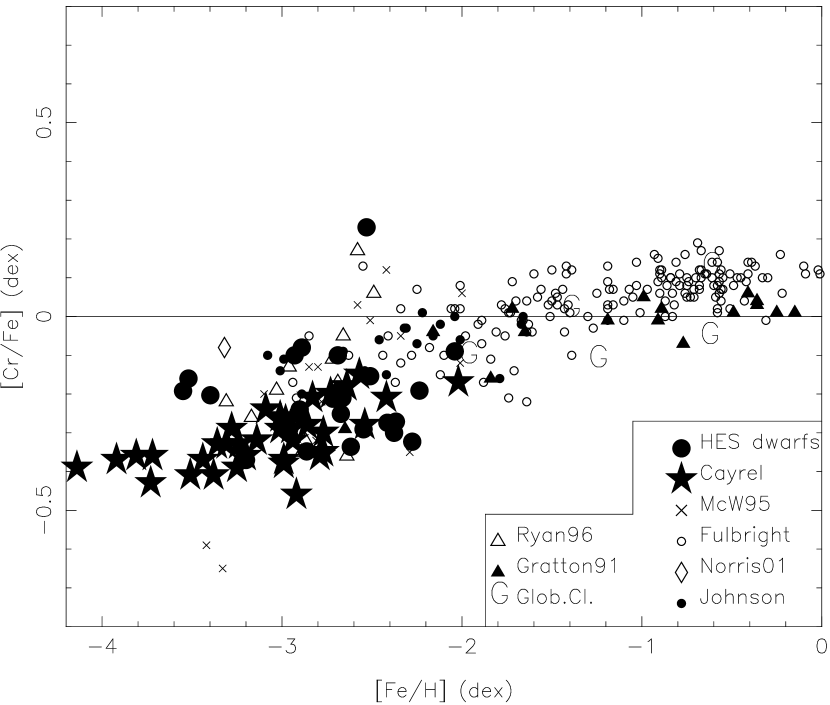
Figure 21: [Cr/Fe] is shown as a function of metallicity for a large sample of halo stars compiled from the literature. The symbol key is shown on the figure and the full references are given in the text.

Figures 20 to 25 present the abundance ratios of Ni, Mg, Ca, Cr, Mn and Co with respect to Fe for this large sample of halo stars over a very wide range in metallicity using our work (ignoring the C-rich stars), that of Cayrel et al. (2003) and the other surveys referenced above. The first of these figures shows the relationship between [Ni/Fe] and metallicity (Figure 20). [Ni/Fe] is constant over the full range of [Fe/H] with a mean value within 0.1 dex of the Solar value and a scatter consistent with the observational errors. Since Ni and Fe are very closely related in terms of the nucleosynthetic origin, their constant ratio is gratifying but expected. The relationship between [Cr/Fe] and metallicity (Figure 21) is reasonably tight and shows a gradual increase of this abundance ratio towards higher metallicity, which explains the difference between the [Cr/Fe] seen among globular clusters and those of the even more metal poor dwarfs from the HES (see Table 11). The scatter is consistent with the measurement errors at all values of [Fe/H].

A similar plot for [Mn/Fe] (Figure 24) shows a similar trend, but also illustrates the tremendous difficulty of combining surveys without delving deeply into the adopted atomic data of each. There clearly are systematic differences in abundance scale between the various surveys displayed. The same comment regarding the difference between the EMP dwarfs and the globular clusters made above for [Cr/Fe] apply here as well.

Plots of the $\alpha$-elements [Ca/Fe] and [Mg/Fe] show an elevated flat plateau extending over most of the metallicity range. Assuming that the stars included with [Fe/H] $>-1$ dex actually are halo stars, these ratios drop to the Solar value at [Fe/H] $>-1$ dex. The [Mg/Fe] plot shows a rather large dispersion at all metallicities, which suggests problems in the atomic data reminiscent of those discussed earlier and increases our reluctance to consider the dispersion and apparent existence of the “small group” with Solar [Mg/Fe] we detect in the HES dwarfs as arising from star-to-star variations in [Mg/Fe].

Figure 25 shows the behavior of [Co/Fe] as a function of metallicity. It is above Solar at the lowest metallicites, but appears to fall to near the Solar value somewhat earlier than do the curves of the $\alpha$-elements.

Real trends in abundance ratios do exist, but they are relatively small and large samples of stars over a wide range in [Fe/H] must be assembled to identify them. Considerable care is required in merging different surveys.

8 Binarity

Field stars of Solar metallicity are well known to often be members of binary systems. Latham et al. (2002) and Carney et al. (2003) find no difference in the binary frequency they establish for moderately metal poor halo populations compared to that of nearby more metal-rich populations; the formal frequency of spectroscopic binaries and multiple systems per target is 17.0$\pm$1.0%. There are several methods to search for such using our data. Examination of the spectra by eye established that HE0218$-$2738 from the Keck Pilot Project is a double lined spectroscopic binary, and that the star HE0024$-$2523 has broadened lines, both reported in Cohen et al. (2002b). Lucatello et al. (2003) determined the orbital parameters for the latter star. A more quantitative test is to examine the cross-correlation of the spectrum over spectral regions selected to be without strong lines to determine the width of the spectral lines. This width is presumably from stellar rotation, but the rotation of main sequence turn off stars is expected to be undetectably small under normal circumstances. For the C-enhanced star HE0024$-$2523, Lucatello et al. (2003) demonstrate that the high rotation is due to tidal synchronization in a close binary.

Figure 17 shows the mean FWHM of the peak of the cross-correlation function, which we denote as $W$, for each star over selected spectral regions devoid of very strong lines. The bright dwarf LP0831$-$07 was used as a template. The stars are ordered by observing run, so any secular trend in the FWHM would be apparent. Recall that the nominal resolving power for the HIRES configuration we use is $R=\lambda/\Delta\lambda=$45,000, which corresponds to $W$ for a single spectrum of 13.3 km s^-1, since the cross-correlation has an expected FWHM twice that of a single star (with unresolved lines). Open circles denote the measurements for the stars from the May 2002 run taken with a slightly wider slit. Most of the stars scatter around the expected value; the few cases slightly below are either measurement error or represent spectra taken during periods of unusually good seeing where the stellar image did not totally fill the slit. But there are some cases with noticably larger $W$, one of which is HE0024$-$2523.

This process led to the discovery of HE0458$-$1346, the star with the largest $W$ in the sample, as a double lined spectroscopic binary, with the secondary component contributing a small fraction of the total light and with a velocity separation at the epoch of observation smaller than that of HE0218$-$2738, which had at the epoch of observation a wider velocity separation, but the second star contributes a very small fraction of the light at optical wavelengths. There are several other stars with unusually large values of $W$, but nothing suspicous was seen when their spectra were checked.

We are monitoring some of these dwarfs, particularly those with C-enhancement, for radial velocity variations. Establishing the the fraction of binary stars for our sample of EMP dwarfs will require substantial additional observational efforts.

9 Comments on Nucleosynthesis

This study of EMP stars together with the very recent work of Cayrel et al. (2003) offer significant improvements upon previous studies in two critically important areas. One, we detect a plateau in the abundance ratios relative to [Fe/H] of very metal-poor dwarf stars for the $\alpha$-elements included in our work between Mg and Ni. In contrast Cr, Mn and Co show definite trends with metallicity. Two, in contrast to previous results showing a large scatter in the abundances, we find a small dispersion in [X/Fe] for these elements. These dispersions are still for many species limited by internal or systematic errors rather than by star-to-star variations in abundance ratios. We discuss the abundance ratios first. The values we infer for our sample of EMP dwarfs from the HES are similar to those found in the previous studies of very metal poor stars by McWilliam et al. (1995), Carretta et al. (2002) and the many additional surveys referred to in §7.5. We adopt the simplest possible hypothesis initially. Such metal poor stars must be very old, and hence the contribution of Type Ia SN to their chemical inventory must be essentially zero. We therefore assume that only Type II SN have contributed to the stellar inventory.

We first compare our deduced abundances with the yields for type II SN taken from the semi-empirical phenomenological calculations of Qian & Wasserburg (2002), which are in fact based on earlier analyses of EMP stars. Figure 18 plots the mean abundance ratios [X/Fe] for our sample of EMP dwarfs as a function of atomic number, with barium plotted at atomic number 46. The large stars denote values from Cayrel et al. (2003) for elements where we have no data (Na and K) or cases where our values disagree with theirs (Si) or our value is particularly uncertain (Zn). In comparing the mean abundances with model predictions, the systematic errors as well as the random ones in the abundance ratios must be included. Hence we combine in quadrature a systematic error of 0.15 dex, allowing an upward change of 0.22 dex as well for Si only (see §7.6), with the error in the mean [X/Fe] from random errors. An additional error term of $\pm$0.15 dex was added for [Al/Fe], due to the large non-LTE corrections applied to Al. These errors are indicated in Figure 18 and also in the next figure. The predictions of Qian & Wasserburg (2002) are indicated in Figure 18 by open circles. These fit the data quite well in general, although Co has a large discrepancy ($\sim 0.8$ dex, more than 4$\sigma$).

Woosley & Weaver (1995) and Umeda & Nomoto (2002), among others, present detailed ab initio calcuations of the yields for low metallicity Type II SN. A comparison with the predictions of abundance ratios with respect to Fe by the latter group for SN with masses of 15, 30 and 50 M_⊙ and explosion energies ranging from 10⁵¹ to 10⁵³ ergs is shown in figure 19. These are representative of the many cases they studied, which cover a range from 13 to 50 M_⊙, with a large range in explosion energy as well. These models have particular difficulty in reproducing the odd-even effect as seen in EMP stars; they often overestimate its magnitude, and so underestimate one or more of the observed [Na/Fe], [Al/Fe], [K/Fe], [Sc/Fe], [Co/Fe] and [Mn/Fe] ratios in EMP stars. In order to reproduce the observations for the Fe-peak elements, Umeda & Nomoto (2004) introduce additional parameters involving fall back and mixing. Some combination of all these parameters does reproduce our data; SN progenitors at the upper end of the mass range considered are required. But why that, and only that, small range of progenitor mass and SN explosion parameters occurs under EMP conditions remains to be explained.

Another important result from our work is in the suggestion of a plateau in the abundance ratios at very low metallicity (i.e. [X/Fe] fixed as [Fe/H] varies) for most elements (particularly the $\alpha$-elements) studied here between Mg and Ni except Cr, Co and Mn. These last three elements show definite trends between [X/Fe] and [Fe/H]. Another element which shows such a trend is Cu (atomic number 29, i.e. another odd element) (see Simmerer et al., 2003, and references therein). Furthermore all of these trends between [X/Fe] and [Fe/H], both flat and with a definite slope, are followed by the Galactic globular clusters (Table 11). We thus require some metallicity or time dependent effect to produce the trends observed for Cr, Mn, Co and Cu, the latter three of which are relatively rare elements with $N$(Co, Mn or Cu)/$N$(Fe) $<100$, while maintaining constant ratios for the abundant $\alpha$-elements.

The bulk of the production of Type II SN is $\alpha$-elements; the production of Mn, Co and Cu is relatively small and, at least as modeled by Umeda & Nomoto (2002) and Umeda & Nomoto (2004), much more subject to variation given small changes in the characteristics of the the progenitor star or the SN explosion. Either the SN yields or the IMF could be metallicity dependent. In the latter case the favored mass for the SN progenitors would evolve monotonically with time, presumably towards smaller masses. The constancy of the abundance ratios for the $\alpha$-elements suggests that the IMF is not varying strongly with time/metallicity, so we suspect that the production yields of some of the less abundant elements in the region of the Fe-peak must be varying with metallicity. Perhaps this is related to neutron excess dependent yields for these specific elements (Arnett, 1971, 1996), with a larger odd-even amplitude for smaller neutron excesses which are characteristic of metal-poor material that has not been modified by H or He burning.

The most crucial result presented here, in addition to the abundance ratios themselves, is the small dispersions found for [X/Fe] for X between Mg and Ni for the EMP dwarfs in our sample once the C-rich stars and the dwarf HE2344$-$2800 are eliminated (see Table 8). These dispersions are consistent with our small estimated observational errors (up to a factor of $\sim$2 larger in many cases, probably arising from the neglect of small systematic effects arising within the atomic data, see §7.4) given in Table 6 and hence the intrinsic dispersions may be even smaller. The only genuine outlier among the dwarfs in our sample is the star HE2344$-$2800 with abnormally high Cr and Mn, as originally pointed out by Carretta et al. (2002). The nucleosynthetic processes required to produce these anomalies is not well understood.

The HES covers a large area on the sky, so different SN presumably contribute to the chemical inventory of each star. As the metallicity decreases and the number of supernovae contributing to a given parcel of gas becomes smaller, this uniformity becomes more challenging to reproduce. Yet the observations appear to demand uniformity in relative yield patters for common elements up to the Fe-peak group. One would expect that different SN in the early halo might have had different mass progenitors and different mass cuts, eject different masses into the ISM, which are then diluted and mixed within the ISM in a very stochastic manner. Their relative yields and yield patterns were not identical, as is found in all SNII nucleosynthesis models. How a diverse class of stars with very different metallicities can exhibit so homogenous a set of abundance ratios from very variable SNII sources is not evident. One possibility is that even the lowest metallicity stars contain the average of ejecta from many SNII, thus smoothing out the effect from different sources. A second possibility is that the early SN were much more uniform in their characteristics. Invoking a Population III pushes the issues of homogeneity further back in time, where perhaps the physics of star formation at very low metallicity could introduce constraints which gave rise to a much sharper IMF, a better defined SN mass, etc. than are characteristic of Type II SN today. The simulations of Karlsson & Gustafsson (2001) illustrate some of the issues involved.

Among the heavy elements, once the C-rich stars are eliminated, most of the dwarfs lie within a range Sr/Fe of about a factor of 10; the full range including a few outliers with very low Sr/Fe is a factor of 80. Ba and Sr are reasonably well correlated with each other when both are detected, but there are five dwarfs in which no line of Ba II was detected. The production of Sr through the $s$-process is discussed at length in Travaglio et al. (2004). Presumably the wide range we see in Sr/Fe and even wider range in Ba/Fe reflects the varying contributions of the $r$ and $s$ neutron capture processes to the chemical inventory of Sr and Ba in EMP dwarfs and of mass transfer across binaries, or perhaps the ratio of Ba to Sr from the $r$-process alone varies somewhat at these low metallicities for reasons not yet understood.

Homogeneity still largely prevails even at these very low metallicities for the more abundant elements Mg through Zn. But for Sr and Ba, which are much rarer elements, with abundances a factor of about 1000 below that of Ni, stochastic effects have become easily visible among these EMP dwarfs.

9.1 The C-rich Stars

These stars are main sequence turnoff stars. They are not blue stragglers. They are unevolved, and so any peculiarities must be primordial, inherent in the ISM when the stars formed, or accreted from some external source such as a binary companion, a nearby SN, etc. Our sample of candidate EMP dwarfs contains two carbon stars and two stars with C strongly enhanced. Detailed analyses have already been published for the two C-enhanced stars HE 2148–1247 (Cohen et al., 2003) and HE 0024–2523 (Lucatello et al., 2003). These stars, and one of the two carbon stars in our sample, HE 0143$-$0441, share the property that in addition to the enhancement of the light elements, the neutron capture elements past the Fe peak are strongly enhanced. Very large enhancements of the $s$-process elements are seen, including detections of lead in all three of these stars. On the other hand, the fourth EMP carbon star, HE0007$-$1832, shows no enhancement of the heavy elements and no detection of lead. It has Sr/Fe and Ba/Fe ratios consistent with the majority of the non-C-enhanced stars (see Figures 9 and 12).

The scenario discussed for such stars is similar to that suggested by McClure (1983) for the Ba stars. It involves mass transfer in a binary system where the primary star has become an AGB star and has transferred mass containing nucleosynthesis debris onto the secondary star, which is the star we now observe. This can explain most of the properties of these stars, and is the origin of our desire to check the C-enhanced stars for binarity as thoroughly as possible. While it is clear from the work of McClure (1990), North, Jorrisen & Mayor (2000) and others that most of the Ba stars are binaries, none of the giant carbon stars with no $s$-process enhancement appear to be binaries (McClure, 1997). There is thus considerable interest in whether or not the EMP stars of this type are binaries; evidence at present is scarce, but see Preston & Sneden (2001), among others.

Detailed models of nucleosynthesis in such systems have been presented by Gallino et al. (1998), Busso, Gallino & Wasserburg (1999), Arlandini et al. (1999) and others. The yield of $s$-nuclei in an AGB star depends on the mass of the star and the magnitude of the carbon pocket. Thus it should be possible to produce a range of enhancements of the $s$-process elements, from very little to very large, as is seen in our sample.

10 Implications for the HES Survey

Every effort has been made to find and include the most metal poor dwarfs possible in choosing the sample from the HES for high resolution observations. As is indicated in §7.1, there are no dwarfs in the present sample with [Fe/H] $<-4$ dex, and very few with [Fe/H] $<-3.5$ dex. Furthermore in our follow up efforts thus far no additional turnoff stars with $\mbox{[Fe/H]}<-3.5$ have yet been identified for future detailed study. This rarity of stars below [Fe/H] $\sim-3.5$ dex must be a genuine characteristic of the general metal poor star population. Cayrel et al. (2003) succeeded in adding two stars to the six previously known to have [Fe/H] $\leq-3.5$ dex, five of which are studied in detail in Norris, Ryan & Beers (2001) and the most iron-poor of all, with [Fe/H] = $-5.3$ dex (found in the HES), is analyzed by Christlieb et al. (2004). We have added two more stars to that select group, HE0218$-$2738 and BS16945-0089, for a total of 10.

The spectra of EMP candidate dwarfs are very weak lined, and the assignment of metallicity from moderate resolution spectra is difficult, yet this is crucial to utilization of the full sample of the HES. We first consider the accuracy of this process as it is currently carried out, as described in Beers, Preston & Shectman (1992) and Beers (1999). We define $\Delta$(Fe) as [Fe/H](HK) $-$ [Fe/H](HIRES). Ideally $\Delta$(Fe) should be 0 for all stars. Ignoring the bright calibration stars, the mean of $\Delta$(Fe) for the 25 dwarfs in our sample computed from the values given in Table 5 is +0.46$\pm$0.31 dex, as can be seen by comparing the middle and bottom panels of Figure 1. If we exclude the 3 stars from the HK survey in our sample, then for 22 stars we find $\Delta$(Fe) = +0.51$\pm$0.23 dex. Excluding the four C-rich stars in our sample only reduces $\Delta$(Fe) to +0.48 dex. Our preliminary impression at this time is that this problem is less severe among the HES giants, which appear to have a mean $\Delta$(Fe) $\approx$ $+0.2$ dex, corresponding to just the difference in adopted Solar iron abundances, although we have noticed that among the HES giant samples, the C-rich stars systematically tend to have abnormally large values of $\Delta$(Fe).

Thus the calibration used by the HES for the approximate abundance indicator [Fe/H](HK), based on a similar parameter used by the HK Survey, appears to systematically underestimate the abundance of EMP candidate dwarfs as measured from our detailed abundance analyses. The variation with time over the past 15 years of concensus choices for the iron abundance of the Sun can give rise to a maximum contribution of +0.2 dex to $\Delta$(Fe). Part of the offset in [Fe/H] scales might also be due to a selection bias similar to the Malmquist bias. The metallicity distribution function of halo stars declines rapidly as [Fe/H] decreases in the metallicity range of interest. Uncertainties in [Fe/H](HK) will tend to scatter intermediate metallicity stars into the low metallicity regime at a rate which greatly exceeds the converse, thus introducing a bias towards positive values of $\Delta$(Fe) and producing a sample of EMP stars selected for high dispersion spectroscopy whose true metallicity is higher than anticipated. Monte Carlo trials suggest that for (Gaussian) uncertainties in [Fe/H](HK) of $\pm$0.3 dex, an increase of $\sim$0.1 dex in the mean [Fe/H] above that expected will result in the HIRES sample. This leaves $\sim$0.2 dex presumably arising from calibration differences, including differences between the $T_{\mbox{\scriptsize eff}}$ scale adopted here and that of Beers et al. (1999).

Irrespective of the cause of this problem, in spite of our best efforts thus far, the samples of candidate EMP dwarfs culled from the HES appear to be contaminated with somewhat higher metallicity, although still very metal poor, dwarfs even after two stages of vetting including moderate resolution spectroscoy.

It is also important to note in this context that the counts of EMP stars within the HK Survey given by Beers (1999) are based almost entirely on moderate resolution spectra, not from detailed abundance analyses from high dispersion spectra. Since dwarfs dominate the samples, Beers’ statement that the HK Survey contains 100 known EMP stars may be a substantial overestimate.

The follow up spectra cannot easily detect the weak molecular features in EMP dwarfs in the $T_{\mbox{\scriptsize eff}}$ range considered here, so the fraction of C-rich stars found among the HIRES sample, which is $\sim$20%, is a lower limit to the fraction of such stars in the full HES sample. This fraction is best established from the giants, but there the issue of internal production cannot be so readily dismissed.

The previously unpublished HES EMP candidates presented here have a median $V$ of $\sim 15.7$ mag. Because these stars are all dwarfs near the TO, they represent a sample of halo dwarfs with median distance of 2.8 kpc, while a giant at the same $V$ with luminosity 1 mag below the RGB tip would be at a distance of 30 kpc. We model the density distribution in the Galactic halo as $\rho\propto R_{GC}^{-3}$, where $R_{GC}$ is the galactocentric radius, to calculate the ratio of dwarfs to giants in the range of magnitude relevant to the HES and to the HK Surveys by viewing the volumes of the two surveys in galactocentric coordinates. At the distances typical of the stars in the HK Survey (which are considerably brighter), the 8 kpc distance to the Galactic center dominates, and $R_{GC}$ does not drop rapidly with increasing magnitude within such a survey. The fainter giants in the HES are far above the Galactic plane, hence the rapid decline in $\rho(R_{GC})$ becomes important, while the dwarfs are still close enough that for them $R_{GC}\approx 8$ kpc and hence $\rho$ is approximately constant. A rough calculation suggests that the number density of giants to dwarfs at the main sequence turnoff at $V=13.5$ is more than a factor of 10 larger than it is at $V=16$. Therefore it will be more challenging in the HES than in the HK Survey to separate the very distant halo giants from dwarfs.

11 Summary

We present the chemical abundances in a sample of 17 candidate extremely metal poor dwarf stars, including 14 previously unpublished EMP candidates from the Hamburg/ESO Survey. This is combined with the dwarfs from the Keck Pilot Project and gives a total sample of 28 EMP candidate dwarfs (22 from the HES) near the main sequence turn off with $T_{\mbox{\scriptsize eff}}$ $\geq 6000$ K.

Dwarfs this hot have very weak atomic and molecular lines, making the problem of finding EMP dwarfs and analyzing their spectra difficult. Only the most abundant elements yield measurable absorption features. But dwarfs have the advantage of being unevolved, with no chance of any interior nuclear processing beyond burning H to He, and thus no chance of self-pollution. We analyze high resolution and high precision spectra of these stars taken with HIRES at the Keck Observatory. Our sample has a median [Fe/H] of $-2.7$ dex, extends to $-3.5$ dex, and is somewhat less metal-poor than was expected from [Fe/H](HK,HES) determined from low resolution spectra. We find, in agreement with previous surveys (see, for example Beers, Preston & Shectman, 1992), that there appears to be a sharp drop in the metallicity distribution of stars below [Fe/H] $=-3$ dex. In our follow up efforts thus far no additional turnoff stars with $\mbox{[Fe/H]}<-3.5$ have yet been identified for future detailed study.

The abundance ratios [X/Fe] which we derive are similar to those found by earlier investigations, and are, with the exception of Si, in good agreement with the very recent results of the First Stars Project (Cayrel et al., 2003) for a large sample of EMP giants. Silicon shows a substantial difference in behavior between the EMP giants and the dwarfs, which may be due in part to problems in the analysis, but is not fully understood at present; Sc/Fe may show a similar, smaller, difference between EMP dwarfs and giants. Ignoring Si, the details of the abundance trends, in particular the existence of an abundance plateau for the $\alpha$-elements with fixed [X/Fe] as [Fe/H] decreases, are better defined than in earlier studies. These abundance ratios are in general in reasonable agreement with predictions using the yields of Qian & Wasserburg (2002) and assuming that only Type II SN contribute to the stellar inventory for these EMP dwarfs. Cr, Co and Mn (and Cu, see Simmerer et al. 2003), show definite trends of mean [X/Fe] with metallicity. These behaviors are all in good agreement with the abundance ratios of Galactic globular clusters.

The dispersions of [X/Fe] are surprisingly small, as was also found by the First Stars Project. They are still in most cases dominated by internal errors. Careful attention to the details of the atomic physics and the analysis will be required for further improvement.

We interpret these trends in abundance ratios as requiring a fixed IMF for the SN progenitors combined with metallicity dependent yields for the low abundance elements such as Mn, Co and Cu. The progenitor mass must be biased towards the high end of the range generally considered for Type II SN to fit the observations. Even at the low metallicities considered here, we suspect that many SN contributed to the chemical inventory of each of the observed stars to reproduce the small dispersions in [X/Fe] determined by us.

Sr/Fe and Ba/Fe have dispersions significantly larger than the elements from Mg to Ni. But by eliminating the C-rich stars, and thus presumably the bulk of the $s$-process material, we reduce the dispersions for these elements.

Two dwarfs in the sample are carbon stars, while two others have significant C enhancements. All four have ¹²C/¹³C $\sim$7. The C-enhanced stars are a mixed group. Three of the four have large enhancements of the heavy neutron capture elements including lead, implying a strong $s$-process contribution, presumably from an AGB companion. The fourth C-rich star shows no anomalies among the heavy elements compared to the bulk of the sample.

We examined the available information regarding the binarity of the sample stars. We pay particular attention to the C-rich stars, since their substantial $s$-process enrichment supposedly arises via mass transfer from an AGB star. To date there are three definite binaries, two double lined systems and one star with an orbit (Lucatello et al., 2003), in our sample.

A sample of EMP giants from the HES will be difficult to assemble, not just because the stars are faint, but because the ratio of giants to dwarfs is falling rapidly in the relevant magnitude regime (13 to 16 mag) due to the rapid drop in stellar density in the halo as a function of galactocentric radius. Such a sample, which we are now constructing, will consist of giants at typical distances of 30 kpc, and will be very interesting to explore.

Table 1: Sample of New Stars

Star	$V$	RA	Dec	$E(B-V)$	Obs.Run	Exp.Time	SNR
	(Mag)	J2000		(Mag)		(sec)
Very bright
LP0831$-$0700	11.62	3 06 05.4	$-$22 19 18	0.019	9/2001	900	$>$100
HK stars
BS16545$-$0089	14.44	11 24 27.6	+36 50 28	0.019	5/2002	1800	80
BS16945$-$0054	13.67	10 50 57.6	+34 01 39	0.022	5/2002	2700	$>$100
HES stars
HE0007$-$1832	15.46	00 09 52.8	$-$18 16 12	0.030	9/2001	8400	90
HE0028$-$2152	15.80	00 31 07.7	$-$21 36 07	0.019	9/2002	9600	100
HE0054$-$2123	15.54	00 56 53.2	$-$21 07 29	0.020	9/2002	8400	100
HE0102$-$0633	15.57	01 05 25.6	$-$06 17 36	0.145	9/2001	10800	90
HE0105$-$2202	15.76	01 07 31.2	$-$21 46 06	0.016	9/2002	3600	65
HE0142+0147	15.60	01 44 47.6	+02 02 17	0.021	9/2001	9600	90
HE0143$-$0441	16.35	01 45 37.8	$-$04 26 43	0.024	9/2002	9600	80
HE0458$-$1346	15.29	05 01 11.7	$-$13 42 04	0.121	9/2002	4800	95
HE0508$-$1555	15.38	05 10 35.4	$-$15 51 39	0.068	9/2002	6000	100
HE1141$-$0610	13.75	11 44 22.6	$-$06 26 59	0.030	5/2002	2700	100
HE1320+0038	13.78	13 22 35.3	+00 22 31	0.021	5/2002	2700	100
HE1346$-$0427	14.20	13 49 25.2	$-$04 42 15	0.029	5/2002	4800	100
HE2209$-$1240	15.76	22 11 48.7	$-$12 25 46	0.036	9/2002	8400	100
HE2341$-$2029	16.25	23 44 19.7	$-$20 13 20	0.027	9/2002	9600	85

Table 2: $W_{\lambda}$ for 17 Candidate Dwarf EMP Stars

Line $\lambda$	Species	EP	Log($gf$)	BS16545	BS16945	LP831$-$70	HE0007	HE0028	HE0054	HE0102$-$0633	HE0105$-$2202	HE0142+0147	HE0143$-$0441	HE0458$-$1346	HE0508$-$1555	HE1141$-$0610	HE1320+0038	HE1346$-$0427	HE2209$-$1240	HE2341$-$2029
(Å)		(eV)		$-$0089	$-$0054		$-$1832	$-$2152	$-$2123
4057.52	12.0	4.34	-1.200	$\cdots$	22.8	11.2	$\cdots$	9.6	7.2	$\cdots$	11.2	$\cdots$	21.2	25.7	17.6	14.1	$\cdots$	$\cdots$	9.6	$\cdots$
4167.28	12.0	4.34	-1.000	$\cdots$	31.8	11.2	$\cdots$	17.6	10.8	$\cdots$	$\cdots$	22.4	$\cdots$	32.2	24.2	28.1	16.0	$\cdots$	16.0	17.0
4703.00	12.0	4.34	-0.670	$\cdots$	55.4	22.8	24.3	37.5	23.4	$\cdots$	36.0	35.2	$\cdots$	46.3	46.0	40.7	27.0	6.4	38.3	35.0
5172.70	12.0	2.71	-0.380	69.2	158.4	111.8	102.8	124.0	124.0	104.3	124.7	128.9	163.5	166.0	132.1	136.6	112.9	69.8	123.3	116.8
5183.62	12.0	2.72	-0.160	80.4	175.6	130.7	130.0	140.5	140.5	117.2	129.8	148.4	187.8	183.4	148.7	149.9	127.6	86.8	145.9	134.0
3944.01	13.0	0.00	-0.640	14.0	75.5	35.8	$\cdots$	49.4	49.4	34.7	34.9	57.8	$\cdots$	82.2	54.2	56.6	36.0	14.9	69.8	41.1
3961.52	13.0	0.00	-0.340	19.6	76.1	62.3	63.0	62.3	62.3	42.0	50.5	65.6	77.8	91.1	67.0	60.3	58.8	21.8	77.3	51.7
3905.53	14.0	1.91	-1.090	36.4	125.6	79.3	$\cdots$	95.7	95.7	82.0	99.0	103.2	239.1	141.0	101.4	84.7	79.5	48.2	96.6	96.9
4226.74	20.0	0.00	0.240	79.8	149.4	85.3	$\cdots$	126.2	126.2	110.4	116.1	116.2	$\cdots$	151.7	129.1	127.9	111.9	74.0	121.4	118.2
4289.37	20.0	1.88	-0.300	$\cdots$	32.8	$\cdots$	$\cdots$	19.7	19.7	$\cdots$	14.4	18.1	$\cdots$	23.8	18.9	16.2	11.2	$\cdots$	14.6	$\cdots$
4302.54	20.0	1.90	0.280	8.4	60.9	15.3	$\cdots$	43.9	43.9	20.3	30.0	41.9	$\cdots$	50.4	43.9	46.3	24.8	10.4	41.1	37.7
4318.66	20.0	1.90	-0.210	$\cdots$	34.2	$\cdots$	$\cdots$	16.0	14.4	7.2	$\cdots$	27.8	$\cdots$	24.2	21.4	15.5	$\cdots$	$\cdots$	17.4	18.0
4425.44	20.0	1.88	-0.360	$\cdots$	25.1	$\cdots$	$\cdots$	9.3	14.4	16.0	$\cdots$	17.6	25.6	30.3	15.3	16.8	13.9	$\cdots$	15.1	17.8
4435.69	20.0	1.89	-0.520	$\cdots$	21.7	$\cdots$	$\cdots$	12.3	12.3	12.8	$\cdots$	$\cdots$	$\cdots$	$\cdots$	8.0	10.4	$\cdots$	$\cdots$	$\cdots$	9.6
4454.79	20.0	1.90	0.260	13.0	53.4	18.0	31.0	44.8	44.8	$\cdots$	31.3	40.7	70.0	48.7	45.5	42.3	27.8	6.4	36.5	33.8
4246.82	21.1	0.32	0.242	12.6	69.5	34.4	$\cdots$	47.0	47.0	34.7	25.7	47.0	$\cdots$	52.5	51.3	56.8	36.2	5.6	42.3	47.2
4314.08	21.1	0.62	-0.100	$\cdots$	37.7	12.0	$\cdots$	23.1	23.1	$\cdots$	16.0	25.2	$\cdots$	20.8	23.6	34.9	13.0	$\cdots$	20.1	20.8
4320.73	21.1	0.60	-0.260	$\cdots$	31.5	7.0	$\cdots$	14.0	12.6	$\cdots$	16.0	24.0	$\cdots$	19.2	17.6	20.3	$\cdots$	$\cdots$	14.6	$\cdots$
4670.41	21.1	1.36	-0.580	$\cdots$	$\cdots$	$\cdots$	$\cdots$	$\cdots$	$\cdots$	$\cdots$	$\cdots$	$\cdots$	11.2	$\cdots$	$\cdots$	$\cdots$	$\cdots$	$\cdots$	$\cdots$	$\cdots$
3958.22	22.0	0.05	-0.160	$\cdots$	25.3	-4.9	$\cdots$	17.6	14.4	$\cdots$	22.4	22.4	34.3	18.7	19.2	14.4	-9.6	$\cdots$	-16.4	$\cdots$
3998.64	22.0	0.05	-0.050	$\cdots$	24.4	-13.0	$\cdots$	16.8	16.8	$\cdots$	20.0	22.4	22.4	27.6	22.4	16.9	$\cdots$	$\cdots$	-22.4	21.7
4533.25	22.0	0.85	0.480	$\cdots$	$\cdots$	-7.0	$\cdots$	12.1	9.0	$\cdots$	$\cdots$	12.8	10.0	10.5	16.4	8.0	$\cdots$	$\cdots$	$\cdots$	11.2
4534.78	22.0	0.84	0.280	$\cdots$	$\cdots$	$\cdots$	$\cdots$	$\cdots$	8.0	$\cdots$	$\cdots$	$\cdots$	$\cdots$	$\cdots$	$\cdots$	4.6	$\cdots$	$\cdots$	$\cdots$	$\cdots$
4548.77	22.0	0.83	-0.350	$\cdots$	$\cdots$	$\cdots$	$\cdots$	$\cdots$	$\cdots$	$\cdots$	$\cdots$	$\cdots$	$\cdots$	5.7	$\cdots$	$\cdots$	$\cdots$	$\cdots$	$\cdots$	$\cdots$
4981.74	22.0	0.85	0.500	$\cdots$	$\cdots$	$\cdots$	$\cdots$	$\cdots$	9.0	$\cdots$	$\cdots$	11.2	28.8	16.0	11.2	8.0	$\cdots$	$\cdots$	$\cdots$	8.0
4999.51	22.0	0.83	0.250	$\cdots$	15.6	$\cdots$	$\cdots$	8.0	9.0	$\cdots$	8.0	$\cdots$	19.2	11.2	13.9	$\cdots$	$\cdots$	$\cdots$	$\cdots$	$\cdots$
3900.54	22.1	1.13	-0.450	25.2	76.3	30.1	$\cdots$	61.8	61.8	35.6	46.1	$\cdots$	66.8	67.8	62.8	79.5	53.6	19.7	54.2	60.5
3987.61	22.1	0.61	-2.730	$\cdots$	11.7	$\cdots$	$\cdots$	$\cdots$	$\cdots$	$\cdots$	$\cdots$	$\cdots$	$\cdots$	$\cdots$	$\cdots$	$\cdots$	$\cdots$	$\cdots$	$\cdots$	$\cdots$
4012.39	22.1	0.57	-1.610	$\cdots$	42.8	6.0	$\cdots$	25.3	25.3	$\cdots$	17.6	20.8	$\cdots$	22.9	22.3	29.5	$\cdots$	$\cdots$	26.0	24.0
4028.35	22.1	1.89	-0.870	$\cdots$	24.0	$\cdots$	$\cdots$	$\cdots$	$\cdots$	$\cdots$	$\cdots$	$\cdots$	29.0	$\cdots$	$\cdots$	12.8	$\cdots$	$\cdots$	$\cdots$	$\cdots$
4300.05	22.1	1.18	-0.490	12.0	74.9	23.4	$\cdots$	56.8	56.8	34.9	33.8	$\cdots$	$\cdots$	61.9	59.7	70.1	48.5	10.4	55.9	49.4
4301.93	22.1	1.16	-1.200	$\cdots$	38.5	8.0	$\cdots$	27.2	27.2	$\cdots$	$\cdots$	24.0	$\cdots$	23.2	18.2	35.2	$\cdots$	$\cdots$	22.9	15.4
4312.86	22.1	1.18	-1.160	$\cdots$	45.7	6.0	$\cdots$	29.8	29.8	$\cdots$	$\cdots$	22.4	$\cdots$	30.4	31.1	34.1	17.6	$\cdots$	$\cdots$	16.0
4395.03	22.1	1.08	-0.510	20.0	78.8	25.6	$\cdots$	60.0	60.0	36.0	46.7	57.4	$\cdots$	62.1	60.2	75.3	51.2	15.7	59.5	54.6
4399.77	22.1	1.24	-1.290	$\cdots$	34.5	$\cdots$	$\cdots$	19.5	19.5	$\cdots$	16.0	$\cdots$	$\cdots$	$\cdots$	20.4	29.7	13.5	$\cdots$	19.1	$\cdots$
4417.72	22.1	1.16	-1.160	$\cdots$	43.8	$\cdots$	$\cdots$	$\cdots$	$\cdots$	$\cdots$	19.2	25.6	$\cdots$	23.5	29.5	27.4	21.9	$\cdots$	$\cdots$	22.3
4443.81	22.1	1.08	-0.700	18.2	72.4	16.3	38.3	58.0	58.0	33.7	43.1	48.6	63.0	57.5	58.6	64.4	46.1	15.7	51.4	49.0
4468.51	22.1	1.13	-0.600	16.8	75.8	22.1	42.1	64.1	64.1	28.8	40.0	44.3	66.0	58.0	61.2	68.4	49.5	9.6	54.7	54.3
4501.28	22.1	1.12	-0.760	15.0	64.9	21.9	43.5	50.7	50.7	$\cdots$	36.9	44.7	55.3	49.4	57.3	59.1	39.1	8.0	48.8	53.5
4533.97	22.1	1.24	-0.640	11.2	68.7	18.2	39.4	43.1	34.3	30.4	32.7	48.5	55.2	55.8	49.5	64.2	38.5	9.6	48.1	41.5
4563.77	22.1	1.22	-0.820	$\cdots$	60.8	14.6	20.0	34.6	32.1	$\cdots$	19.2	35.3	43.0	$\cdots$	45.8	51.7	30.5	6.4	37.8	37.2
4571.98	22.1	1.57	-0.340	11.2	63.2	28.0	31.6	46.4	46.4	26.1	$\cdots$	51.0	70.3	49.2	50.4	63.5	43.5	12.8	47.2	19.2
4589.95	22.1	1.24	-1.650	$\cdots$	24.0	$\cdots$	$\cdots$	8.0	$\cdots$	$\cdots$	$\cdots$	$\cdots$	$\cdots$	16.0	11.2	14.4	$\cdots$	$\cdots$	8.0	$\cdots$
4798.54	22.1	1.08	-2.670	$\cdots$	12.8	$\cdots$	$\cdots$	$\cdots$	$\cdots$	$\cdots$	$\cdots$	$\cdots$	$\cdots$	$\cdots$	$\cdots$	$\cdots$	$\cdots$	$\cdots$	$\cdots$	$\cdots$
5185.91	22.1	1.89	-1.460	$\cdots$	16.0	$\cdots$	$\cdots$	$\cdots$	$\cdots$	$\cdots$	$\cdots$	$\cdots$	$\cdots$	$\cdots$	$\cdots$	$\cdots$	$\cdots$	$\cdots$	$\cdots$	$\cdots$
4111.77	23.0	0.30	0.408	$\cdots$	$\cdots$	$\cdots$	$\cdots$	-9.4	$\cdots$	-7.2	$\cdots$	$\cdots$	$\cdots$	$\cdots$	$\cdots$	-6.4	$\cdots$	$\cdots$	$\cdots$	$\cdots$
4254.33	24.0	0.00	-0.110	14.0	63.7	24.6	$\cdots$	49.7	49.7	28.9	40.2	45.7	$\cdots$	61.3	48.6	51.5	38.5	9.0	49.6	45.0
4274.79	24.0	0.00	-0.230	9.8	66.8	18.2	$\cdots$	37.5	37.5	23.2	29.5	32.4	$\cdots$	59.9	41.1	36.0	32.4	12.8	43.8	30.2
4289.72	24.0	0.00	-0.361	7.0	57.9	22.7	$\cdots$	37.7	37.7	$\cdots$	$\cdots$	33.6	$\cdots$	44.5	37.7	39.6	27.5	12.8	36.4	30.2
5206.04	24.0	0.94	0.030	$\cdots$	38.8	7.0	11.8	22.5	22.5	10.0	19.2	$\cdots$	24.0	30.2	17.7	25.5	9.6	$\cdots$	25.0	15.0
4030.75	25.0	0.00	-0.470	-7.0	72.2	10.9	27.5	29.6	18.0	12.2	20.8	36.6	45.0	46.4	28.8	24.5	14.4	-5.0	31.5	20.4
4033.06	25.0	0.00	-0.620	$\cdots$	44.3	8.4	20.0	16.0	9.0	9.9	12.8	21.2	24.0	24.7	20.1	18.0	16.0	-5.0	26.9	17.0
3865.52	26.0	1.01	-0.980	24.7	83.8	53.3	$\cdots$	64.0	64.0	63.2	69.2	67.1	65.3	85.4	61.5	$\cdots$	55.0	28.9	70.3	62.8
3895.67	26.0	0.11	-1.670	$\cdots$	95.9	57.9	$\cdots$	68.0	68.0	51.9	64.6	77.0	$\cdots$	84.6	71.8	74.2	$\cdots$	39.2	75.6	72.0
3899.72	26.0	0.09	-1.530	38.9	94.2	61.0	53.0	74.7	74.7	61.1	78.2	78.4	79.8	85.0	74.1	73.5	62.9	43.4	74.5	72.8
3902.96	26.0	1.56	-0.470	$\cdots$	82.8	49.2	62.4	58.5	58.5	59.2	67.4	67.0	82.5	78.8	66.3	64.6	49.6	28.0	66.3	59.7
3906.49	26.0	0.11	-2.240	$\cdots$	72.7	39.9	$\cdots$	45.6	45.6	$\cdots$	54.4	49.7	79.7	66.2	54.2	37.9	29.0	15.0	51.2	42.4
3916.74	26.0	3.24	-0.560	$\cdots$	17.4	$\cdots$	$\cdots$	$\cdots$	$\cdots$	$\cdots$	$\cdots$	$\cdots$	$\cdots$	$\cdots$	$\cdots$	19.1	$\cdots$	$\cdots$	$\cdots$	$\cdots$
3920.27	26.0	0.12	-1.750	27.8	90.5	58.1	$\cdots$	73.3	73.3	60.3	72.8	75.0	72.1	82.0	71.4	74.3	71.2	31.4	$\cdots$	71.7
3922.92	26.0	0.05	-1.650	47.8	90.8	65.3	66.9	74.7	74.7	63.2	68.7	84.0	86.5	81.5	77.9	78.4	66.2	42.6	75.5	79.6
3930.31	26.0	0.09	-1.590	44.9	$\cdots$	61.7	$\cdots$	85.0	85.0	69.7	$\cdots$	82.8	$\cdots$	$\cdots$	90.0	$\cdots$	73.0	52.7	79.8	$\cdots$
3949.96	26.0	2.18	-1.160	$\cdots$	26.5	$\cdots$	$\cdots$	9.6	16.0	$\cdots$	$\cdots$	$\cdots$	$\cdots$	25.5	$\cdots$	$\cdots$	$\cdots$	$\cdots$	$\cdots$	11.0
4005.24	26.0	1.56	-0.610	$\cdots$	80.8	$\cdots$	50.5	62.3	62.3	45.5	51.6	58.8	68.2	80.4	62.5	71.8	57.5	20.8	64.7	$\cdots$
4045.81	26.0	1.49	0.280	65.5	136.2	86.9	86.5	105.0	105.0	83.8	100.8	106.3	116.2	120.0	109.9	112.0	98.6	67.5	103.1	91.3
4063.59	26.0	1.56	0.060	50.0	108.1	73.6	69.1	85.4	85.4	72.5	86.1	80.9	105.1	102.6	89.1	95.1	86.8	50.2	89.0	87.1
4071.74	26.0	1.61	-0.020	41.3	94.4	69.1	70.5	77.8	77.8	68.8	80.0	81.3	87.6	93.7	79.3	88.5	77.9	45.6	80.6	77.6
4118.55	26.0	3.57	0.140	$\cdots$	42.1	8.0	$\cdots$	18.7	18.7	11.9	$\cdots$	14.4	34.0	34.0	19.7	19.2	7.6	$\cdots$	14.1	15.0
4132.06	26.0	1.61	-0.820	21.0	83.2	42.5	$\cdots$	59.4	59.4	33.7	50.3	53.6	63.9	72.8	59.3	62.5	48.8	19.8	58.7	56.0
4143.87	26.0	1.56	-0.620	21.0	86.5	49.8	$\cdots$	63.6	63.6	49.0	64.2	66.5	63.9	79.0	68.4	65.8	57.1	26.4	70.7	64.8
4147.67	26.0	1.49	-2.100	$\cdots$	26.9	$\cdots$	$\cdots$	$\cdots$	$\cdots$	$\cdots$	$\cdots$	$\cdots$	$\cdots$	$\cdots$	8.0	$\cdots$	$\cdots$	$\cdots$	$\cdots$	$\cdots$
4172.76	26.0	0.96	-3.070	$\cdots$	11.4	$\cdots$	$\cdots$	$\cdots$	$\cdots$	$\cdots$	$\cdots$	$\cdots$	$\cdots$	$\cdots$	$\cdots$	$\cdots$	$\cdots$	$\cdots$	$\cdots$	$\cdots$
4174.92	26.0	0.91	-2.970	$\cdots$	8.0	$\cdots$	$\cdots$	$\cdots$	$\cdots$	$\cdots$	$\cdots$	$\cdots$	$\cdots$	7.6	$\cdots$	$\cdots$	$\cdots$	$\cdots$	$\cdots$	$\cdots$
4181.75	26.0	2.83	-0.370	$\cdots$	43.1	14.0	$\cdots$	$\cdots$	16.2	$\cdots$	25.6	22.6	$\cdots$	33.6	27.6	33.5	17.6	$\cdots$	19.7	34.6
4187.05	26.0	2.45	-0.550	$\cdots$	43.6	21.9	$\cdots$	25.9	25.9	$\cdots$	22.4	30.8	$\cdots$	40.6	28.7	30.1	17.6	$\cdots$	28.5	25.6
4187.81	26.0	2.43	-0.550	$\cdots$	46.5	$\cdots$	$\cdots$	30.0	30.0	$\cdots$	32.9	33.4	$\cdots$	43.0	34.5	37.9	22.6	11.4	29.9	$\cdots$
4198.33	26.0	2.40	-0.720	$\cdots$	49.6	15.6	$\cdots$	$\cdots$	20.9	$\cdots$	17.6	30.0	$\cdots$	46.3	30.3	32.5	24.8	$\cdots$	35.4	22.1
4199.10	26.0	3.05	0.160	$\cdots$	51.6	20.5	$\cdots$	29.8	29.8	$\cdots$	27.3	$\cdots$	$\cdots$	45.3	41.5	37.8	$\cdots$	8.8	36.4	28.0
4202.04	26.0	1.49	-0.710	22.3	85.5	45.4	$\cdots$	63.2	63.2	39.4	48.8	62.7	$\cdots$	79.9	64.3	59.5	56.3	24.5	63.8	58.9
4216.19	26.0	0.00	-3.360	$\cdots$	33.1	$\cdots$	$\cdots$	13.2	13.2	$\cdots$	$\cdots$	12.3	$\cdots$	25.3	16.0	$\cdots$	$\cdots$	$\cdots$	$\cdots$	$\cdots$
4222.22	26.0	2.45	-0.970	$\cdots$	31.4	$\cdots$	$\cdots$	10.4	10.4	$\cdots$	9.6	$\cdots$	$\cdots$	25.2	6.6	$\cdots$	$\cdots$	$\cdots$	$\cdots$	$\cdots$
4227.44	26.0	3.33	0.270	$\cdots$	55.5	14.4	$\cdots$	$\cdots$	20.6	24.0	20.4	22.3	$\cdots$	47.6	32.3	34.1	$\cdots$	6.7	$\cdots$	28.6
4233.61	26.0	2.48	-0.600	$\cdots$	45.0	17.6	$\cdots$	20.8	20.8	$\cdots$	18.5	25.5	$\cdots$	36.0	29.0	32.5	$\cdots$	$\cdots$	28.6	22.4
4235.95	26.0	2.43	-0.340	11.2	65.8	28.5	$\cdots$	34.8	34.8	25.9	44.3	38.5	$\cdots$	49.1	44.8	$\cdots$	29.1	10.9	44.7	38.2
4250.13	26.0	2.47	-0.410	$\cdots$	58.7	19.6	$\cdots$	33.7	33.7	20.5	29.9	36.3	$\cdots$	55.0	34.7	35.1	29.3	$\cdots$	36.5	35.1
4250.80	26.0	1.56	-0.380	20.4	74.4	42.0	$\cdots$	53.7	53.7	44.8	50.5	59.0	$\cdots$	70.3	62.9	61.8	52.2	19.5	59.6	50.0
4260.49	26.0	2.40	0.140	18.2	76.8	40.0	$\cdots$	55.2	55.2	39.8	53.5	54.2	$\cdots$	69.8	62.5	60.0	49.7	24.1	61.8	50.6
4271.16	26.0	2.45	-0.350	$\cdots$	55.9	22.4	$\cdots$	32.7	32.7	25.7	32.4	25.8	$\cdots$	46.4	38.2	32.9	20.9	9.0	31.0	31.5
4271.77	26.0	1.49	-0.160	45.8	96.3	68.9	$\cdots$	76.4	76.4	68.0	76.9	77.7	$\cdots$	93.0	85.0	81.7	76.9	42.5	81.3	74.2
4282.41	26.0	2.18	-0.780	$\cdots$	51.6	22.6	$\cdots$	26.8	26.8	$\cdots$	25.0	25.6	$\cdots$	38.4	37.0	31.6	20.8	$\cdots$	28.4	$\cdots$
4294.14	26.0	1.49	-0.970	$\cdots$	81.4	34.8	$\cdots$	62.1	62.1	35.5	53.9	58.8	$\cdots$	74.3	61.7	71.1	47.7	$\cdots$	58.4	51.8
4299.25	26.0	2.43	-0.350	$\cdots$	71.3	21.9	$\cdots$	40.3	40.3	15.9	31.0	35.1	$\cdots$	53.9	43.2	54.2	27.3	11.2	35.6	36.8
4307.91	26.0	1.56	-0.070	53.3	$\cdots$	$\cdots$	$\cdots$	$\cdots$	$\cdots$	77.4	95.6	103.7	$\cdots$	116.1	112.3	$\cdots$	94.3	48.8	108.6	97.1
4325.77	26.0	1.61	0.010	41.2	103.2	67.1	$\cdots$	77.9	77.9	64.3	69.3	83.8	$\cdots$	93.5	86.2	92.9	80.5	47.4	78.2	80.0
4375.94	26.0	0.00	-3.030	$\cdots$	49.7	$\cdots$	$\cdots$	14.4	8.0	$\cdots$	19.2	22.3	$\cdots$	21.7	17.9	12.0	$\cdots$	4.7	23.7	$\cdots$
4383.56	26.0	1.49	0.200	62.5	122.4	81.6	$\cdots$	104.1	104.1	84.7	100.9	92.7	$\cdots$	121.6	102.4	118.9	98.3	63.2	107.7	97.9
4404.76	26.0	1.56	-0.140	46.9	102.2	67.4	$\cdots$	82.2	82.2	72.3	77.7	82.3	$\cdots$	101.8	84.5	89.9	79.7	46.8	86.9	81.4
4415.13	26.0	1.61	-0.610	14.6	88.3	47.4	$\cdots$	62.4	62.4	52.0	57.4	59.6	$\cdots$	70.0	66.5	67.6	54.3	26.5	65.5	54.1
4427.32	26.0	0.05	-3.040	$\cdots$	52.4	14.4	$\cdots$	22.9	22.9	10.1	22.8	20.7	56.1	36.0	23.6	$\cdots$	$\cdots$	$\cdots$	25.9	$\cdots$
4430.62	26.0	2.22	-1.660	$\cdots$	14.7	$\cdots$	$\cdots$	$\cdots$	$\cdots$	$\cdots$	$\cdots$	$\cdots$	$\cdots$	17.0	$\cdots$	$\cdots$	$\cdots$	$\cdots$	$\cdots$	$\cdots$
4442.35	26.0	2.20	-1.250	$\cdots$	39.6	$\cdots$	$\cdots$	21.0	21.0	15.3	17.0	$\cdots$	$\cdots$	27.2	25.2	$\cdots$	$\cdots$	$\cdots$	14.8	11.2
4447.73	26.0	2.22	-1.340	$\cdots$	29.7	$\cdots$	$\cdots$	9.1	9.1	$\cdots$	11.1	17.7	29.5	25.0	13.4	$\cdots$	$\cdots$	$\cdots$	$\cdots$	$\cdots$
4459.14	26.0	2.18	-1.280	$\cdots$	40.1	$\cdots$	$\cdots$	18.3	18.3	$\cdots$	15.2	12.8	16.0	25.0	14.4	$\cdots$	$\cdots$	$\cdots$	$\cdots$	16.0
4461.66	26.0	0.09	-3.210	$\cdots$	41.7	$\cdots$	$\cdots$	18.8	18.8	$\cdots$	$\cdots$	$\cdots$	24.0	28.8	19.3	$\cdots$	$\cdots$	$\cdots$	18.1	$\cdots$
4489.75	26.0	0.12	-3.970	$\cdots$	10.4	$\cdots$	$\cdots$	$\cdots$	$\cdots$	$\cdots$	$\cdots$	$\cdots$	$\cdots$	$\cdots$	$\cdots$	$\cdots$	$\cdots$	$\cdots$	$\cdots$	$\cdots$
4494.57	26.0	2.20	-1.140	$\cdots$	30.9	$\cdots$	$\cdots$	16.8	16.8	$\cdots$	14.4	16.0	21.6	32.8	23.4	20.6	$\cdots$	$\cdots$	20.8	15.0
4531.16	26.0	1.49	-2.150	$\cdots$	23.0	$\cdots$	$\cdots$	$\cdots$	$\cdots$	$\cdots$	$\cdots$	$\cdots$	16.0	17.0	11.2	$\cdots$	$\cdots$	$\cdots$	$\cdots$	$\cdots$
4592.66	26.0	1.56	-2.450	$\cdots$	12.0	$\cdots$	$\cdots$	$\cdots$	$\cdots$	$\cdots$	$\cdots$	$\cdots$	$\cdots$	$\cdots$	$\cdots$	$\cdots$	$\cdots$	$\cdots$	$\cdots$	$\cdots$
4602.95	26.0	1.49	-2.220	$\cdots$	21.6	$\cdots$	$\cdots$	$\cdots$	$\cdots$	$\cdots$	10.0	$\cdots$	$\cdots$	$\cdots$	$\cdots$	$\cdots$	$\cdots$	$\cdots$	$\cdots$	$\cdots$
4871.33	26.0	2.86	-0.360	$\cdots$	44.1	$\cdots$	$\cdots$	30.5	30.5	$\cdots$	14.4	22.7	37.2	37.2	25.5	29.6	$\cdots$	$\cdots$	$\cdots$	15.0
4872.14	26.0	2.88	-0.570	$\cdots$	32.8	$\cdots$	$\cdots$	22.7	22.7	$\cdots$	$\cdots$	14.4	27.9	36.3	20.5	$\cdots$	18.1	$\cdots$	$\cdots$	$\cdots$
4891.50	26.0	2.85	-0.110	$\cdots$	55.4	16.8	$\cdots$	30.0	30.0	21.4	37.4	$\cdots$	47.9	49.0	32.7	34.9	29.6	$\cdots$	32.1	30.3
4919.00	26.0	2.86	-0.340	$\cdots$	$\cdots$	11.2	$\cdots$	17.5	17.5	11.3	10.9	20.2	20.8	$\cdots$	17.9	22.4	10.4	$\cdots$	22.8	$\cdots$
4920.51	26.0	2.83	0.150	$\cdots$	60.8	22.1	32.5	38.3	38.3	$\cdots$	31.2	40.4	61.5	55.9	41.0	39.3	30.8	9.6	45.6	35.2
4957.61	26.0	2.81	0.230	$\cdots$	74.4	36.3	45.6	56.6	56.6	37.2	46.5	51.2	69.3	70.8	62.0	75.1	48.7	16.3	72.1	46.7
5083.34	26.0	0.96	-2.960	$\cdots$	$\cdots$	$\cdots$	$\cdots$	$\cdots$	$\cdots$	$\cdots$	$\cdots$	$\cdots$	$\cdots$	8.0	7.1	$\cdots$	$\cdots$	$\cdots$	$\cdots$	$\cdots$
5166.28	26.0	0.00	-4.200	$\cdots$	$\cdots$	$\cdots$	$\cdots$	$\cdots$	$\cdots$	$\cdots$	$\cdots$	$\cdots$	$\cdots$	5.0	$\cdots$	$\cdots$	$\cdots$	$\cdots$	$\cdots$	$\cdots$
5171.61	26.0	1.48	-1.790	$\cdots$	49.1	$\cdots$	$\cdots$	17.6	15.0	$\cdots$	18.3	19.9	$\cdots$	31.4	24.3	12.8	$\cdots$	$\cdots$	25.2	11.2
5192.35	26.0	3.00	-0.420	$\cdots$	$\cdots$	4.5	$\cdots$	11.2	$\cdots$	$\cdots$	14.6	16.0	30.4	$\cdots$	12.8	9.6	$\cdots$	$\cdots$	16.0	11.2
5194.95	26.0	1.56	-2.090	$\cdots$	$\cdots$	$\cdots$	$\cdots$	8.0	$\cdots$	$\cdots$	$\cdots$	$\cdots$	17.7	$\cdots$	$\cdots$	$\cdots$	$\cdots$	$\cdots$	$\cdots$	$\cdots$
5216.28	26.0	1.61	-2.150	$\cdots$	16.0	$\cdots$	$\cdots$	$\cdots$	$\cdots$	$\cdots$	$\cdots$	$\cdots$	$\cdots$	12.8	$\cdots$	10.1	$\cdots$	$\cdots$	$\cdots$	$\cdots$
5217.40	26.0	3.21	-1.070	$\cdots$	$\cdots$	$\cdots$	$\cdots$	4.6	$\cdots$	$\cdots$	$\cdots$	$\cdots$	$\cdots$	$\cdots$	$\cdots$	$\cdots$	$\cdots$	$\cdots$	$\cdots$	$\cdots$
5227.19	26.0	1.56	-1.350	$\cdots$	$\cdots$	24.7	$\cdots$	47.0	47.0	$\cdots$	42.3	41.3	43.5	58.9	47.5	44.3	31.6	$\cdots$	53.4	43.0
5232.95	26.0	2.94	-0.100	$\cdots$	49.6	19.0	18.8	$\cdots$	17.2	11.8	33.3	31.5	46.7	38.2	33.6	34.2	23.8	$\cdots$	35.5	34.8
5269.55	26.0	0.86	-1.320	16.8	94.9	51.3	43.0	66.3	66.3	56.4	67.8	66.3	87.4	85.6	66.5	63.2	50.0	28.4	63.3	60.7
5324.19	26.0	3.21	-0.100	$\cdots$	41.8	$\cdots$	$\cdots$	$\cdots$	$\cdots$	$\cdots$	$\cdots$	19.8	$\cdots$	$\cdots$	$\cdots$	$\cdots$	$\cdots$	$\cdots$	$\cdots$	13.6
4178.86	26.1	2.57	-2.530	$\cdots$	21.2	$\cdots$	$\cdots$	$\cdots$	$\cdots$	11.2	$\cdots$	$\cdots$	$\cdots$	12.0	8.0	23.5	8.5	$\cdots$	11.2	$\cdots$
4233.17	26.1	2.57	-2.000	8.4	48.4	13.4	$\cdots$	24.4	24.4	14.7	27.2	30.4	$\cdots$	26.9	31.3	53.3	28.6	$\cdots$	30.4	30.3
4416.82	26.1	2.77	-2.430	$\cdots$	17.7	$\cdots$	$\cdots$	$\cdots$	$\cdots$	$\cdots$	$\cdots$	$\cdots$	$\cdots$	8.0	$\cdots$	8.0	$\cdots$	$\cdots$	11.2	$\cdots$
4491.40	26.1	2.84	-2.600	$\cdots$	12.8	$\cdots$	$\cdots$	8.0	$\cdots$	$\cdots$	$\cdots$	$\cdots$	$\cdots$	$\cdots$	$\cdots$	$\cdots$	$\cdots$	$\cdots$	$\cdots$	$\cdots$
4508.30	26.1	2.84	-2.280	$\cdots$	20.5	$\cdots$	$\cdots$	$\cdots$	$\cdots$	$\cdots$	$\cdots$	13.4	16.0	7.0	$\cdots$	16.1	11.4	$\cdots$	$\cdots$	$\cdots$
4555.89	26.1	2.82	-2.170	$\cdots$	26.6	7.0	$\cdots$	11.2	8.0	$\cdots$	$\cdots$	14.4	16.8	$\cdots$	15.0	22.7	12.8	$\cdots$	16.0	$\cdots$
4583.84	26.1	2.81	-2.020	$\cdots$	48.4	11.9	18.0	20.0	17.0	13.0	16.0	22.9	28.2	34.9	31.3	36.0	32.7	$\cdots$	33.5	27.1
4923.93	26.1	2.88	-1.320	$\cdots$	58.8	16.8	30.7	35.9	35.9	19.0	32.2	36.0	49.1	45.1	41.2	66.3	45.6	10.4	40.3	28.9
5018.45	26.1	2.89	-1.220	12.6	68.5	28.3	35.4	45.0	45.0	33.1	38.2	44.6	55.3	51.7	53.8	73.9	53.2	9.6	53.0	47.5
5197.58	26.1	3.23	-2.230	$\cdots$	16.0	$\cdots$	$\cdots$	$\cdots$	$\cdots$	$\cdots$	$\cdots$	$\cdots$	$\cdots$	$\cdots$	$\cdots$	14.4	$\cdots$	$\cdots$	$\cdots$	$\cdots$
3842.05	27.0	0.92	-0.763	$\cdots$	16.0	$\cdots$	$\cdots$	$\cdots$	$\cdots$	$\cdots$	$\cdots$	$\cdots$	$\cdots$	22.4	$\cdots$	$\cdots$	$\cdots$	-5.0	$\cdots$	$\cdots$
3845.46	27.0	0.92	0.009	-8.0	41.9	14.0	24.3	19.2	16.0	15.0	26.0	32.0	43.8	26.5	24.0	16.2	16.0	-5.0	27.7	24.0
3873.11	27.0	0.43	-0.666	-7.0	47.0	14.0	$\cdots$	20.4	10.0	$\cdots$	$\cdots$	27.8	$\cdots$	32.7	21.2	19.8	8.0	$\cdots$	18.4	$\cdots$
4121.31	27.0	0.92	-0.315	$\cdots$	20.2	14.9	$\cdots$	16.0	$\cdots$	8.0	14.4	20.0	$\cdots$	24.2	$\cdots$	$\cdots$	$\cdots$	$\cdots$	12.8	17.0
3858.30	28.0	0.42	-0.967	22.4	69.4	31.9	36.8	53.3	53.3	42.8	38.4	57.8	52.7	63.4	53.8	53.6	39.6	19.1	57.0	38.3
4401.55	28.0	3.19	0.084	$\cdots$	11.0	$\cdots$	$\cdots$	$\cdots$	$\cdots$	$\cdots$	$\cdots$	$\cdots$	$\cdots$	$\cdots$	$\cdots$	$\cdots$	$\cdots$	$\cdots$	$\cdots$	$\cdots$
4810.54	30.0	4.08	-0.170	$\cdots$	$\cdots$	$\cdots$	$\cdots$	-6.4	5.4	-6.0	$\cdots$	$\cdots$	10.4	$\cdots$	$\cdots$	$\cdots$	$\cdots$	$\cdots$	$\cdots$	-6.4
4077.71	38.1	0.00	0.170	36.6	93.1	5.4	72.3	66.3	66.3	45.5	56.1	70.9	136.2	91.1	85.7	89.8	50.0	21.4	76.8	66.9
4215.52	38.1	0.00	-0.140	20.6	84.9	$\cdots$	$\cdots$	50.5	50.5	37.5	45.3	60.2	$\cdots$	74.9	76.3	76.7	37.6	18.6	68.0	61.0
4130.65	56.1	2.72	0.560	$\cdots$	$\cdots$	$\cdots$	$\cdots$	$\cdots$	$\cdots$	$\cdots$	$\cdots$	$\cdots$	60.5	$\cdots$	$\cdots$	$\cdots$	$\cdots$	$\cdots$	$\cdots$	$\cdots$
4554.04	56.1	0.00	0.170	-7.0	57.9	-3.0	23.1	15.9	20.0	$\cdots$	11.2	21.8	195.8	47.4	31.9	37.5	8.0	4.8	34.7	11.2
4934.16	56.1	0.00	-0.150	-7.0	47.2	$\cdots$	$\cdots$	8.0	9.0	12.0	11.2	15.9	180.7	36.7	20.0	24.7	9.0	4.8	22.4	7.0
3950.36	39.1	0.10	-0.490	$\cdots$	$\cdots$	$\cdots$	$\cdots$	8.0	$\cdots$	-8.0	$\cdots$	$\cdots$	18.3	$\cdots$	$\cdots$	$\cdots$	$\cdots$	$\cdots$	$\cdots$	$\cdots$
4883.69	39.1	1.08	0.070	$\cdots$	$\cdots$	$\cdots$	$\cdots$	$\cdots$	$\cdots$	$\cdots$	$\cdots$	$\cdots$	18.9	$\cdots$	$\cdots$	$\cdots$	$\cdots$	$\cdots$	$\cdots$	$\cdots$
4496.97	40.1	0.71	-0.590	$\cdots$	$\cdots$	$\cdots$	$\cdots$	$\cdots$	$\cdots$	$\cdots$	$\cdots$	$\cdots$	14.4	$\cdots$	$\cdots$	$\cdots$	$\cdots$	$\cdots$	$\cdots$	$\cdots$
3988.52	57.1	0.40	0.210	$\cdots$	$\cdots$	$\cdots$	$\cdots$	$\cdots$	$\cdots$	$\cdots$	$\cdots$	$\cdots$	44.5	$\cdots$	$\cdots$	$\cdots$	$\cdots$	$\cdots$	$\cdots$	$\cdots$
3995.75	57.1	0.17	-0.060	$\cdots$	$\cdots$	$\cdots$	$\cdots$	$\cdots$	$\cdots$	$\cdots$	$\cdots$	$\cdots$	34.2	$\cdots$	$\cdots$	$\cdots$	$\cdots$	$\cdots$	$\cdots$	$\cdots$
4086.71	57.1	0.00	-0.070	$\cdots$	$\cdots$	$\cdots$	$\cdots$	$\cdots$	$\cdots$	$\cdots$	$\cdots$	$\cdots$	44.0	$\cdots$	$\cdots$	$\cdots$	$\cdots$	$\cdots$	$\cdots$	$\cdots$
4123.23	57.1	0.32	0.130	$\cdots$	$\cdots$	$\cdots$	$\cdots$	$\cdots$	$\cdots$	$\cdots$	$\cdots$	$\cdots$	30.9	$\cdots$	$\cdots$	$\cdots$	$\cdots$	$\cdots$	$\cdots$	$\cdots$
4333.76	57.1	0.17	-0.060	$\cdots$	$\cdots$	$\cdots$	$\cdots$	$\cdots$	$\cdots$	$\cdots$	$\cdots$	-19.2	$\cdots$	$\cdots$	$\cdots$	$\cdots$	$\cdots$	$\cdots$	$\cdots$	$\cdots$
4073.47	58.1	0.48	0.320	$\cdots$	$\cdots$	$\cdots$	$\cdots$	$\cdots$	$\cdots$	$\cdots$	$\cdots$	$\cdots$	25.6	$\cdots$	$\cdots$	$\cdots$	$\cdots$	$\cdots$	$\cdots$	$\cdots$
4083.23	58.1	0.70	0.240	$\cdots$	$\cdots$	$\cdots$	$\cdots$	$\cdots$	$\cdots$	$\cdots$	$\cdots$	$\cdots$	20.1	$\cdots$	$\cdots$	$\cdots$	$\cdots$	$\cdots$	$\cdots$	$\cdots$
4562.37	58.1	0.48	0.330	$\cdots$	$\cdots$	$\cdots$	$\cdots$	$\cdots$	$\cdots$	$\cdots$	$\cdots$	$\cdots$	18.0	$\cdots$	$\cdots$	$\cdots$	$\cdots$	$\cdots$	$\cdots$	$\cdots$
4061.09	60.1	0.47	0.300	$\cdots$	$\cdots$	$\cdots$	$\cdots$	$\cdots$	$\cdots$	$\cdots$	$\cdots$	$\cdots$	29.7	$\cdots$	$\cdots$	$\cdots$	$\cdots$	$\cdots$	$\cdots$	$\cdots$
4109.46	60.1	0.32	0.180	$\cdots$	$\cdots$	$\cdots$	$\cdots$	$\cdots$	$\cdots$	$\cdots$	$\cdots$	$\cdots$	38.4	$\cdots$	$\cdots$	$\cdots$	$\cdots$	$\cdots$	$\cdots$	$\cdots$
4232.38	60.1	0.06	-0.350	$\cdots$	-11.0	$\cdots$	$\cdots$	$\cdots$	$\cdots$	$\cdots$	$\cdots$	$\cdots$	$\cdots$	$\cdots$	$\cdots$	$\cdots$	$\cdots$	$\cdots$	$\cdots$	$\cdots$
4446.39	60.1	0.20	-0.630	$\cdots$	$\cdots$	$\cdots$	$\cdots$	$\cdots$	-4.0	$\cdots$	$\cdots$	$\cdots$	$\cdots$	$\cdots$	$\cdots$	$\cdots$	$\cdots$	$\cdots$	$\cdots$	$\cdots$
4462.99	60.1	0.56	-0.070	$\cdots$	$\cdots$	$\cdots$	$\cdots$	$\cdots$	$\cdots$	$\cdots$	$\cdots$	$\cdots$	29.6	$\cdots$	$\cdots$	$\cdots$	$\cdots$	$\cdots$	$\cdots$	$\cdots$
3819.67	63.1	0.00	0.510	$\cdots$	-16.0	$\cdots$	-5.0	$\cdots$	$\cdots$	$\cdots$	$\cdots$	$\cdots$	30.4	$\cdots$	$\cdots$	$\cdots$	$\cdots$	$\cdots$	$\cdots$	$\cdots$
3907.11	63.1	0.21	0.170	$\cdots$	$\cdots$	$\cdots$	-5.0	$\cdots$	$\cdots$	$\cdots$	$\cdots$	$\cdots$	22.4	$\cdots$	$\cdots$	$\cdots$	$\cdots$	$\cdots$	$\cdots$	$\cdots$
4129.70	63.1	0.00	0.220	$\cdots$	-10.0	-4.0	-5.0	-10.0	-9.0	-12.8	-11.0	-8.0	22.8	-10.0	-10.0	-5.0	-8.0	-5.0	-11.2	-10.0
4057.81	82.0	1.32	-0.22	$\cdots$	$\cdots$	$\cdots$	$\cdots$	$\cdots$	$\cdots$	$\cdots$	$\cdots$	$\cdots$	48.0	$\cdots$	$\cdots$	$\cdots$	$\cdots$

Table 3: Stellar Parameters

Star	$T_{\mbox{\scriptsize eff}}$	log($g$)	[Fe/H]	$v_{t}$	$v_{r}$	Notes
	(K)	dex	dex	(km s-1)	(km s-1)
Very bright
BD 3$-$740	6355	4.0	$\cdots$	1.4	+174.5	kp
G139$-$8	6200	4.5	$\cdots$	1.0	$-$114.0	b,kp
LP0831$-$0700	6270	4.5	$-3.0$	1.6	$-48.2$
HK stars
BS16545$-$0089	6115	3.6	$-3.0$	1.7	$-163.5$
BS16945$-$0054	6065	3.7	$-2.5$	1.6	$-$73.5
BS17447$-$029	6350	4.4	$\cdots$	1.9	$-201.6$	b,kp
HES stars
HE0007$-$1832	6515	3.8	$-3.0$	1.7	+26.4	cs
HE0024$-$2523	6625	4.3	$-2.5$	1.4	f	f,kp
HE0028$-$2152	6150	3.6	$-2.5$	1.6	+162.5
HE0054$-$2123	6470	4.4	$-2.5$	1.7	+61.2	b
HE0102$-$0633	6350	3.8	$-2.5$	1.7	+3.8
HE0105$-$2202	6330	4.4	$-$3.0	1.6	$-77.3$	b
HE0130$-$2303	6560	4.3	$\cdots$	1.3	+74.2	kp
HE0142+0147	6250	3.7	$-2.5$	1.6	$-97.1$
HE0143$-$0441	6370	4.4	$-3.0$	1.6	+121.8	cs
HE0148$-$2611	6550	4.5	$\cdots$	0.8	$-$223.1	kp
HE0218$-$2738	6550	4.3	$\cdots$	0.8	+134.0	e,kp
HE0242$-$0732	6455	4.6	$\cdots$	0.4	$-188.9$	kp
HE0458$-$1346	6210	4.5	$-2.5$	1.6	+359.4	b
HE0508$-$1555	6365	4.4	$-3.0$	1.6	+88.5	b
HE1141$-$0610	6730	4.0	$-2.5$	1.9	+91.9
HE1320+0038	6500	3.7	$-2.5$	1.9	+22.0
HE1346$-$0427	6205	4.5	$-3.0$	1.6	$-49.0$
HE2133$-$1426	6300	4.5	$\cdots$	1.3	+19.6	c,kp
HE2148$-$1247	6380	3.9	$-2.5$	1.7	+40.6	g
HE2209$-$1240	6240	3.7	$-3.0$	1.6	+22.1
HE2341$-$2029	6500	4.4	$-3.0$	1.6	$-83.0$
HE2344$-$2800	6625	4.3	$\cdots$	1.4	$-$135.8	d,kp

Notes to table 3 are repeated here, as they fall off the end of the page with the table.

a. The [Fe/H] in dex of the model from the Kurucz (1993) grid of model stellar atmospheres used in the analysis.

b. Star just below the main sequence turnoff.

c. log(g) value from Keck Pilot project slightly adjusted.

d. This is a rediscovery of CS 22966$-$048, originally found in the HK Survey.

e. The HIRES spectra of this star are double lined.

f. Spectroscopic binary with known orbit, Lucatello et al. (2003).

g. See Cohen et al. (2003) for a detailed discussion of this peculiar star.

h. $T_{\mbox{\scriptsize eff}}$ obtained from $T(exc)$ for Fe I.

cs. Carbon star; spectrum shows bands of C₂.

kp. From the Keck Pilot Project

Table 4a: Abundances of the Sample Stars

Species	LP0831-070			BS16545$-$0089			BS16945$-$0054			HE0007$-$1832			HE0028$-$2152
	log$\epsilon(X)$	No.	$\sigma$	log$\epsilon(X)$	No.	$\sigma$	log$\epsilon(X)$	No.	$\sigma$	log$\epsilon(X)$	No.	$\sigma$	log$\epsilon(X)$	No.	$\sigma$
	(dex)	Lines	(dex)	(dex)	Lines	(dex)	(dex)	Lines	(dex)	(dex)	Lines	(dex)	(dex)	Lines	(dex)
6.0	$\cdots$	$\cdots$	$\cdots$	$\cdots$	$\cdots$	$\cdots$	$\cdots$	$\cdots$	$\cdots$	8.29	1	$\cdots$	$\cdots$	$\cdots$	$\cdots$
7.0	$\cdots$	$\cdots$	$\cdots$	$\cdots$	$\cdots$	$\cdots$	$\cdots$	$\cdots$	$\cdots$	7.00	1	$\cdots$	$\cdots$	$\cdots$	$\cdots$
12.0	5.33	5	0.23	4.38	2	0.02	5.71	5	0.21	5.65	5	0.35	5.42	5	0.23
13.0	3.64	2	0.07	2.91	2	0.09	3.87	2	0.21	3.28	1	$\cdots$	3.57	2	0.12
14.0	4.70	1	$\cdots$	3.88	1	$\cdots$	5.33	1	$\cdots$	S5.06	1	$\cdots$	4.89	1	$\cdots$
20.0	3.52	3	0.17	3.26	3	0.16	4.27	7	0.11	4.03	1	$\cdots$	4.01	7	0.14
21.1	0.62	3	0.07	$-$0.29	1	$\cdots$	0.90	3	0.01	$\cdots$	$\cdots$	$\cdots$	0.52	3	0.08
22.0	U 2.73	3	0.18	$\cdots$	$\cdots$	$\cdots$	3.04	3	0.07	$\cdots$	$\cdots$	$\cdots$	2.87	4	0.08
22.1	2.36	12	0.12	1.83	8	0.12	3.06	19	0.18	2.73	9	0.15	2.62	14	0.10
23.0	$\cdots$	$\cdots$	$\cdots$	$\cdots$	$\cdots$	$\cdots$	$\cdots$	$\cdots$	$\cdots$	$\cdots$	$\cdots$	$\cdots$	U 2.30	1	$\cdots$
24.0	2.46	4	0.11	1.93	3	0.05	3.07	4	0.09	$\cdots$	$\cdots$	$\cdots$	2.74	4	0.10
25.0	1.80	2	0.02	1.43	1	$\cdots$	2.62	2	0.35	2.51	2	0.03	2.03	2	0.15
26.0	4.59	43	0.13	3.90	21	0.14	5.17	64	0.16	4.80	19	0.19	4.73	55	0.17
26.1	4.67	5	0.19	4.00	2	0.24	5.14	10	0.12	4.88	3	0.21	4.67	6	0.16
27.0	2.66	3	0.17	2.13	2	0.11	2.91	4	0.23	2.95	1	$\cdots$	2.59	3	0.13
28.0	3.29	1	$\cdots$	U 2.91	1	$\cdots$	3.86	2	0.08	3.62	1	$\cdots$	3.52	1	$\cdots$
30.0	$\cdots$	$\cdots$	$\cdots$	$\cdots$	$\cdots$	$\cdots$	$\cdots$	$\cdots$	$\cdots$	$\cdots$	$\cdots$	$\cdots$	U 2.47	1	$\cdots$
38.1	$-$1.55	1	$\cdots$	U $-$0.90	2	0.06	0.50	2	0.06	0.39	1	$\cdots$	$-$0.27	2	0.07
39.1	$\cdots$	$\cdots$	$\cdots$	$\cdots$	$\cdots$	$\cdots$	$\cdots$	$\cdots$	$\cdots$	$\cdots$	$\cdots$	$\cdots$	$-$0.14	1	$\cdots$
56.1	U $-$1.55	1	$\cdots$	U $-$1.38	2	0.20	$-$0.16	2	0.03	$-$0.36	1	$\cdots$	$-$1.18	2	0.04
57.1	$\cdots$	$\cdots$	$\cdots$	$\cdots$	$\cdots$	$\cdots$	$\cdots$	$\cdots$	$\cdots$	U 0.30	1	$\cdots$	$\cdots$	$\cdots$	$\cdots$
60.1	$\cdots$	$\cdots$	$\cdots$	$\cdots$	$\cdots$	$\cdots$	U 0.70	1	$\cdots$	$\cdots$	$\cdots$	$\cdots$	$\cdots$	$\cdots$	$\cdots$
63.1	U $-$0.88	1	$\cdots$	$\cdots$	$\cdots$	$\cdots$	U $-$1.09	2	0.01	U $-$0.35	1	$\cdots$	U $-$0.85	1	$\cdots$
82.0	$\cdots$	$\cdots$	$\cdots$	$\cdots$	$\cdots$	$\cdots$	$\cdots$	$\cdots$	$\cdots$	U 2.34	1	$\cdots$	$\cdots$	$\cdots$	$\cdots$

Table 4b: Abundances of the Sample Stars

Species	HE0054$-$2123			HE0102$-$0633			HE0105$-$2202			HE0142+0147			HE0143$-$0441
	log$\epsilon(X)$	No.	$\sigma$	log$\epsilon(X)$	No.	$\sigma$	log$\epsilon(X)$	No.	$\sigma$	log$\epsilon(X)$	No.	$\sigma$	log$\epsilon(X)$	No.	$\sigma$
	(dex)	Lines	(dex)	(dex)	Lines	(dex)	(dex)	Lines	(dex)	(dex)	Lines	(dex)	(dex)	Lines	(dex)
6.0	$\cdots$	$\cdots$	$\cdots$	$\cdots$	$\cdots$	$\cdots$	$\cdots$	$\cdots$	$\cdots$	$\cdots$	$\cdots$	$\cdots$	7.89	1	$\cdots$
7.0	$\cdots$	$\cdots$	$\cdots$	$\cdots$	$\cdots$	$\cdots$	$\cdots$	$\cdots$	$\cdots$	$\cdots$	$\cdots$	$\cdots$	5.60	1	$\cdots$
12.0	5.36	5	0.14	5.05	2	0.03	5.47	4	0.29	5.53	4	0.16	5.85	3	0.17
13.0	3.79	2	0.12	3.47	2	0.12	3.61	2	0.05	3.72	2	0.13	4.06	1	$\cdots$
14.0	5.11	1	$\cdots$	4.79	1	$\cdots$	5.16	1	$\cdots$	5.16	1	$\cdots$	S 5.20	1	$\cdots$
20.0	4.17	7	0.12	3.89	5	0.28	4.02	4	0.11	4.11	6	0.13	4.60	2	0.17
21.1	0.92	3	0.10	0.33	1	$\cdots$	0.75	3	0.25	$\cdots$	$\cdots$	$\cdots$	1.79	1	$\cdots$
22.0	3.05	6	0.11	$\cdots$	$\cdots$	$\cdots$	3.19	3	0.16	3.02	4	0.16	3.39	5	0.26
22.1	2.99	13	0.12	2.31	7	0.07	2.75	11	0.13	2.63	11	0.09	3.27	8	0.16
23.0	$\cdots$	$\cdots$	$\cdots$	U 2.34	1	$\cdots$	$\cdots$	$\cdots$	$\cdots$	$\cdots$	$\cdots$	$\cdots$	$\cdots$	$\cdots$	$\cdots$
24.0	3.01	4	0.09	2.53	3	0.06	2.83	3	0.15	2.72	3	0.09	3.14	1	$\cdots$
25.0	2.05	2	0.14	1.86	2	0.03	2.13	2	0.08	2.29	2	0.14	2.55	2	0.22
26.0	4.94	56	0.18	4.55	36	0.15	4.90	53	0.18	4.83	53	0.14	5.29	30	0.21
26.1	4.90	5	0.10	4.51	5	0.26	4.92	4	0.17	4.77	6	0.17	5.24	5	0.11
27.0	2.63	2	0.02	2.49	2	0.03	2.86	2	0.03	2.90	3	0.07	3.27	1	$\cdots$
28.0	3.79	1	$\cdots$	3.48	1	$\cdots$	3.48	1	$\cdots$	3.73	1	$\cdots$	3.82	1	$\cdots$
30.0	2.61	1	$\cdots$	U 2.55	1	$\cdots$	$\cdots$	$\cdots$	$\cdots$	$\cdots$	$\cdots$	$\cdots$	2.96	1	$\cdots$
38.1	0.12	2	0.05	$-$0.49	2	0.09	$-$0.02	2	0.04	0.00	2	0.00	1.59	1	$\cdots$
39.1	$\cdots$	$\cdots$	$\cdots$	U 0.03	1	$\cdots$	$\cdots$	$\cdots$	$\cdots$	$\cdots$	$\cdots$	$\cdots$	0.87	2	0.21
40.1	$\cdots$	$\cdots$	$\cdots$	$\cdots$	$\cdots$	$\cdots$	$\cdots$	$\cdots$	$\cdots$	$\cdots$	$\cdots$	$\cdots$	1.68	1	$\cdots$
56.1	$-$0.64	2	0.09	$-$0.82	1	$\cdots$	$-$0.79	2	0.20	$-$0.81	2	0.08	2.28	3	0.18
57.1	$\cdots$	$\cdots$	$\cdots$	$\cdots$	$\cdots$	$\cdots$	$\cdots$	$\cdots$	$\cdots$	U 0.27	1	$\cdots$	0.95	4	0.14
58.1	$\cdots$	$\cdots$	$\cdots$	$\cdots$	$\cdots$	$\cdots$	$\cdots$	$\cdots$	$\cdots$	$\cdots$	$\cdots$	$\cdots$	1.52	3	0.21
60.1	U 1.11	1	$\cdots$	$\cdots$	$\cdots$	$\cdots$	$\cdots$	$\cdots$	$\cdots$	$\cdots$	$\cdots$	$\cdots$	1.71	3	0.20
63.1	U $-$0.45	1	$\cdots$	U $-$0.54	1	$\cdots$	U $-$0.37	1	$\cdots$	U $-$0.87	1	$\cdots$	0.00	3	0.17
82.0	$\cdots$	$\cdots$	$\cdots$	$\cdots$	$\cdots$	$\cdots$	$\cdots$	$\cdots$	$\cdots$	$\cdots$	$\cdots$	$\cdots$	3.29	1	$\cdots$

Table 4c: Abundances of the Sample Stars

Species	HE0458$-$1346			HE0508$-$1555			HE1141$-$0610			HE1320+0038			HE1346$-$0427
	log$\epsilon(X)$	No.	$\sigma$	log$\epsilon(X)$	No.	$\sigma$	log$\epsilon(X)$	No.	$\sigma$	log$\epsilon(X)$	No.	$\sigma$	log$\epsilon(X)$	No.	$\sigma$
	(dex)	Lines	(dex)	(dex)	Lines	(dex)	(dex)	Lines	(dex)	(dex)	Lines	(dex)	(dex)	Lines	(dex)
12.0	5.65	5	0.31	5.70	5	0.28	5.82	5	0.13	5.40	4	0.19	4.54	3	0.25
13.0	4.06	2	0.14	3.91	2	0.09	4.03	2	0.19	3.70	2	0.03	3.02	2	0.08
14.0	5.43	1	$\cdots$	5.23	1	$\cdots$	5.04	1	$\cdots$	4.77	1	$\cdots$	4.17	1	$\cdots$
20.0	4.19	6	0.17	4.22	7	0.11	4.33	7	0.08	3.98	5	0.12	3.16	3	0.19
21.1	0.92	3	0.05	1.02	3	0.03	1.11	3	0.12	0.48	2	0.02	$-$0.33	1	$\cdots$
22.0	3.06	6	0.18	3.23	5	0.14	3.16	5	0.17	U 2.98	1	$\cdots$	$\cdots$	$\cdots$	$\cdots$
22.1	3.00	13	0.11	3.08	15	0.10	3.14	16	0.09	2.61	12	0.05	2.02	9	0.12
23.0	$\cdots$	$\cdots$	$\cdots$	$\cdots$	$\cdots$	$\cdots$	U 2.60	1	$\cdots$	$\cdots$	$\cdots$	$\cdots$	$\cdots$	$\cdots$	$\cdots$
24.0	3.03	4	0.08	2.99	4	0.04	3.24	4	0.13	2.80	4	0.07	2.07	3	0.22
25.0	2.32	2	0.22	2.35	2	0.05	2.55	2	0.01	2.17	2	0.14	U 1.42	2	0.11
26.0	5.08	61	0.18	5.07	60	0.17	5.21	47	0.18	4.79	41	0.15	4.05	33	0.13
26.1	5.04	7	0.18	5.13	6	0.17	5.26	9	0.16	4.83	7	0.14	4.07	2	0.09
27.0	3.01	4	0.28	2.92	2	0.11	3.05	2	0.25	2.62	2	0.07	U 2.31	2	0.54
28.0	3.80	1	$\cdots$	3.83	1	$\cdots$	4.00	1	$\cdots$	3.54	1	$\cdots$	2.92	1	$\cdots$
38.1	0.59	2	0.10	0.75	2	0.04	0.67	2	0.04	$-$0.42	2	0.04	$-$0.76	2	0.15
56.1	$-$0.19	2	0.04	$-$0.35	2	0.01	$-$0.13	2	0.01	$-$1.06	2	0.25	$-$1.22	2	0.20
63.1	U $-$0.51	1	$\cdots$	U $-$0.40	1	$\cdots$	U $-$0.71	1	$\cdots$	U $-$0.72	1	$\cdots$	U $-$0.80	1	$\cdots$

Table 4d: Abundances of the Sample Stars

Species	HE2209$-$1240			HE2341$-$2029			Sun
	log$\epsilon(X)$	No.	$\sigma$	log$\epsilon(X)$	No.	$\sigma$	log$\epsilon(X)$
	(dex)	Lines	(dex)	(dex)	Lines	(dex)	(dex)
6.0	$\cdots$	$\cdots$	$\cdots$	$\cdots$	$\cdots$	$\cdots$	8.39
7.0	$\cdots$	$\cdots$	$\cdots$	$\cdots$	$\cdots$	$\cdots$	7.80
12.0	5.43	5	0.20	5.56	4	0.22	7.54
13.0	3.91	2	0.14	3.79	2	0.11	6.47
14.0	4.95	1	$\cdots$	5.28	1	$\cdots$	7.55
20.0	3.98	6	0.08	4.24	6	0.09	6.36
21.1	0.50	3	0.08	1.02	2	0.03	3.10
22.0	U 2.93	2	0.04	3.15	3	0.21	4.99
22.1	2.62	13	0.05	2.96	13	0.18	4.99
24.0	2.75	4	0.09	2.98	4	0.08	5.67
25.0	2.15	2	0.03	2.36	2	0.03	5.39
26.0	4.78	49	0.17	5.04	47	0.16	7.45
26.1	4.87	7	0.15	5.07	4	0.27	7.45
27.0	2.56	3	0.08	3.03	2	0.07	4.92
28.0	3.58	1	$\cdots$	3.64	1	$\cdots$	6.25
30.0	$\cdots$	$\cdots$	$\cdots$	U 2.78	1	$\cdots$	4.60
38.1	0.13	2	0.03	0.40	2	0.09	2.90
56.1	$-$0.66	2	0.01	$-$0.78	2	0.04	2.13
63.1	U $-$0.78	1	$\cdots$	U $-$0.32	1	$\cdots$	0.51

Table 5: Fe Abundances – Preliminary Estimates vs. Detailed Analyses

Star	[Fe/H]	[Fe/H]	Mod. Res.	Star	[Fe/H]	[Fe/H]	Mod. Res.
	(HK)	(Keck)	Spec		(HK)	(Keck)	Spec
	(dex)	(dex)			(dex)	(dex)
Very bright
BD 3$-$740	$\cdots$	$-$2.69	$\cdots$	G139$-$8	$\cdots$	$-$2.04	$\cdots$
LP0831$-$0700	$\cdots$	$-$2.86	$\cdots$
HK stars
BS16545$-$0089	$\leq-3.0$	$-3.55$	$\cdots$	BS16945$-$0054	$-$3.00	$-2.28$	$\cdots$
BS17447$-$029	$-$3.15	$-$2.91	KPP
HES stars
HE0007$-$1832	$-3.00$	$-2.65$	ESO	HE0024$-$2523	$-$3.08	$-$2.72	KPP
HE0028$-$2152	$-$3.00	$-$2.72	ESO	HE0054$-$2123	$-$3.24	$-$2.51	ESO
HE0102$-$0633	$-$3.30	$-$2.81	LCO	HE0105$-$2202	$-3.00$	$-$2.55	ESO
HE0130$-$2303	$-$3.15	$-$2.93	KPP	HE0142+0147	$-$3.10	$-$2.62	ESO
HE0143$-$0441	$-$3.01	$-$2.16	P200	HE0148$-$2611	$-$3.42	$-$2.96	KPP
HE0218$-$2738	$-$3.81	$-$3.52	KPP	HE0242$-$0732	$-$3.59	$-$3.20	KPP
HE0458$-$1346	$-$2.61	$-$2.37	P200	HE0508$-$1555	$-$2.84	$-$2.38	P200
HE1141$-$0610	$-$3.15	$-$2.24	ESO	HE1320+0038	$-$3.38	$-$2.66	ESO
HE1346$-$0427	$-$3.79	$-$3.40	ESO	HE2133$-$1426	$-$3.32	$-$2.89	KPP
HE2148$-$1247	$-$3.24	$-$2.32	ESO	HE2209$-$1240	$-$2.98	$-$2.67	P200
HE2341$-$2029	$-3.31$	$-2.41$	P200	HE2344$-$2800	$-$3.06	$-2.53$	KPP

Table 6: Abundance Changes for Small Changes in Stellar Parameters

Species	${\Delta}$log$\epsilon(X)$	${\Delta}$log$\epsilon(X)$	$\Delta$log$\epsilon(X)$	$\Delta$log$\epsilon(X)$	[X/Fe]
	($T_{\mbox{\scriptsize eff}}$$+250$K)	(log($g$)$+0.5$ dex)	(Model[Fe/H])$+0.5$ dex)	($v_{t}+0.2$ km s-1)	1 Star
	(dex)	(dex)	(dex)	(dex)	(1$\sigma$)(dex)
Mg I	$-$0.17	0.11	0.13	0.03	0.06
Al I	$-$0.22	0.07	0.14	0.06	0.08
Si I	$-$0.29	0.20	0.17	0.07	0.12
Ca I	$-$0.17	0.04	0.13	0.02	0.05
Sc II	$-$0.13	$-$0.17	0.07	0.01	0.06
Ti I	$-$0.22	0.00	0.10	0.00	0.03
Ti II	$-$0.10	$-$0.17	0.08	0.03	0.05
Cr I	$-$0.24	0.01	0.11	0.04	0.06
Mn I	$-$0.26	0.00	0.11	0.02	0.06
Fe I	$-$0.23	0.03	0.12	0.06	0.13
Fe II	$-$0.04	$-$0.17	0.07	0.02	0.15
Co I	$-$0.25	0.00	0.10	0.01	0.04
Ni I	$-$0.26	0.02	0.12	0.09	0.12
Sr II	$-$0.18	$-$0.11	0.13	0.16	0.18
Ba II	$-$0.17	$-$0.15	0.08	0.04	0.09
Eu II	$-$0.15	$-$0.16	0.06	0.00	0.09

Table 7: Slopes of Mean Abundance Ratios [X/Fe] Versus [Fe/H] for the 28 Candidate EMP Dwarfs

Species	No C-rich Stars
	Slope	No. of	$\sigma$
	(dex/dex)	Stars	(dex)
[Mg/Fe]	$+0.03\pm 0.06$	24	0.20
[Al/Fe]	$-0.23\pm 0.06$	24	0.12
[Si/Fe]	$+0.03\pm 0.06$	19	0.14
[Ca/Fe]	$-0.13\pm 0.05$	24	0.13
[Sc/Fe]	$-0.01\pm 0.05$	23	0.16
[Ti/Fe]	$+0.00\pm 0.05$	24	0.11
[Cr/Fe]	$+0.02\pm 0.05$	24	0.15
[Mn/Fe]	$-0.07\pm 0.10$	19	0.19
[Co/Fe]	$-0.23\pm 0.15$	13	0.11
[Ni/Fe]	$-0.20\pm 0.07$	15	0.09

Table 8: Mean Abundance Ratios [X/Fe] and Their Dispersions for the 28 Candidate EMP Dwarfs

Species	All Stars			No C-enh. Stars			Special Cases
	$<$[X/Fe]$>$	$\sigma$	Num.	$<$[X/Fe]$>$	$\sigma$	Num.	$<$[X/Fe]$>$	$\sigma$	Num.
	(dex)	(dex)	Stars	(dex)	(dex)	Stars	(dex)	(dex)	Stars
Mg/Fe	+0.42	0.22	28	+0.39	0.21	24	+0.56	0.12	20
Mg/Fe	+0.56	0.18	19	+0.52	0.21	19	+0.56	0.15	16
Al/Fe	$-$0.10	0.19	28	$-$0.09	0.16	24	$\cdots$	$\cdots$	$\cdots$
Si/Fe	+0.14	0.17	23	$+0.04$	0.14	19	$\cdots$	$\cdots$	$\cdots$
Ca/Fe	+0.33	0.13	28	+0.31	0.12	24	$\cdots$	$\cdots$	$\cdots$
Sc/Fe	+0.28	0.21	26	+0.24	0.16	23	$\cdots$	$\cdots$	$\cdots$
Ti/Fe	+0.36	0.12	28	+0.36	0.12	24	$\cdots$	$\cdots$	$\cdots$
Cr/Fe	$-$0.23	0.13	27	$-$0.21	0.13	24	$-$0.23	0.09	23
Mn/Fe	$-0.54$	0.20	23	$-0.55$	0.20	19	$-$0.59	0.13	18
Co/Fe	+0.43	0.14	16	+0.42	0.12	13	$\cdots$	$\cdots$	$\cdots$
Ni/Fe	$-$0.03	0.13	18	$-$0.02	0.12	15	$\cdots$	$\cdots$	$\cdots$
Zn/Fe	$0.52$	0.01	2	+0.52	$\cdots$	1	$\cdots$	$\cdots$	$\cdots$
Sr/Fe	$-$0.24	0.53	28	$-$0.37	0.45	24	$-$0.19	0.25	21
Y/Fe	+0.68	0.24	3	+0.40	$\cdots$	1	$\cdots$	$\cdots$	$\cdots$
Ba/Fe	+0.01	0.89	23	$-$0.32	0.35	19	$-$0.20	0.28	16
La/Fe	+2.02	0.22	3	$\cdots$	$\cdots$	$\cdots$	$\cdots$	$\cdots$	$\cdots$
Eu/Fe	$+1.83$	0.17	2	$\cdots$	$\cdots$	$\cdots$	$\cdots$	$\cdots$	$\cdots$
Pb/Fe	+3.32	0.17	3	$\cdots$	$\cdots$	$\cdots$	$\cdots$	$\cdots$	$\cdots$

Table 9: Line-By-Line Values of Mg Abundances

Wavelength	$\Delta$[log$\epsilon$(Mg)]	$\sigma$
(Å)	(dex)	(dex)
4057.5	+0.07	0.04
4167.3	+0.07	0.02
4703.0	+0.12	0.03
5172.7	$-0.13$	0.03
5183.6	$-0.12$	0.03

Table 10: Comparison of Mean Abundance Ratios and Dispersions With Those of Cayrel et al. (2003)

Species	Mean [X/Fe]	Mean [X/Fe]	$\Delta$	$\sigma$	$\sigma$
	EMP Dwarfs	Cayrel Giants	(Dwarfs-Giants)	EMP Dwarfs	Cayrel Giants
	(dex)	(dex)	(dex)	(dex)	(dex)
Mg/Fe	+0.39	+0.28	+0.11	0.13	0.13
Al/Fe	$-0.09$	$-$0.08	$-$0.01	0.16	0.18
Si/Fe	$+0.04$	+0.45	$-0.41$	0.14	0.15
Ca/Fe	+0.31	+0.34	$-0.03$	0.12	0.10
Sc/Fe	+0.24	+0.08	+0.16	0.16	0.11
Ti/Fe	+0.36	+0.23	+0.13	0.12	0.09
Cr/Fe	$-0.21$	$-0.35$	+0.14	0.09	0.05
Mn/Fe	$-0.55$	$-0.44$	$-0.11$	0.13	0.12
Co/Fe	+0.42	+0.27	+0.15	0.12	0.13
Ni/Fe	$-0.02$	$-0.04$	+0.02	0.12	0.11

Table 11: Comparison With Galactic Globular Clusters

	EMP Dwarfs		NGC 6397	M3	M5	M71	47 Tuc
Species	$<$[X/Fe]$>$	$\sigma$[X/Fe]	$<$[X/Fe]$>$	$<$[X/Fe]$>$	$<$[X/Fe]$>$	$<$[X/Fe]$>$	$<$[X/Fe]$>$
	(dex)	(dex)	(dex)	(dex)	(dex)	(dex)	(dex)
[Fe/H]	$-2.66$	$\cdots$	$-2.02$	$-1.45$	$-1.30$	$-0.68$	$-0.67$
[Mg/Fe]	0.39	0.21	0.04	0.22	0.29	0.35	0.40
[Al/Fe]	$-0.09$	0.16	$\cdots$	0.51	0.45	+0.22	+0.27
[Si/Fe]	$+0.04$	0.14	$\cdots$	0.30	0.21	0.27	0.30
[Ca/Fe]	+0.31	0.12	0.24	0.23	0.33	0.36	0.20
[Sc/Fe]	+0.24	0.16	0.27	$-$0.11	0.05	0.03	0.13
[Ti/Fe]	+0.36	0.12	0.47	0.16	0.16	0.23	0.32
[Cr/Fe]	$-0.23$	0.09	$-0.12$	0.00	$-$0.13	$-0.07$	+0.11
[Mn/Fe]	$-0.59$	0.13	$\cdots$	$-$0.37	$-0.39$	$-0.28$	$-0.29$
[Co/Fe]	+0.42	0.12	$\cdots$	0.00	$-$0.06	$-0.07$	$\cdots$
[Ni/Fe]	$-0.02$	0.12	$-0.03$	$-$0.05	$-0.12$	0.01	0.06
[Ba/Fe]	$\sim$ $-0.3$	$\sim$0.3	$-0.24$	+0.21	$-$0.08	+0.19	$\cdots$

Figure 1: A histogram in metallicity as indicated by [Fe/H](HK) for the entire set of dwarf EMP stars isolated from the HES is shown in the upper panel. The middle panel shows the sample chosen for high dispersion observations at Keck. The lower panel shows the [Fe/H] determined from the detailed abundance analysis for the set of stars displayed in the middle panel. The arrow in the lower panel indicates the probable magnitude of the shift of the metallicity scales due to different choices of the Solar Fe abundance.

Figure 2: The ionization equilibrium of Fe is shown as a function of Fe abundance for 27 of the candidate EMP dwarfs in our sample with 1$\sigma$ error bars. The open circles denote the subgiants, while the filled circles indicate the stars below the main sequence turn off. The symbol key for the C-enhanced stars is that used throughout this paper; C stars are shown as large stars, while the C-rich stars are circled.

Figure 3: A synthesis for the region of the CH band near 4320 Å (thin line) is shown superposed on the spectrum of the dwarf C star HE 0007$-$1832 (thick line). The region of the bandhead of C₂ near 5160 Å is shown in the lower panel.

Figure 4: The abundance ratios of Mg (top panel), Al (middle panel) and Si (bottom panel) are shown with respect to Fe for the sample of 28 candidate EMP dwarfs. The symbol key for the C-enhanced stars is that of Figure 2. The dashed horizontal line is the Solar ratio. A typical 1$\sigma$ uncertainty for each abundance ratio is shown for the most metal poor star in each panel. The vertical range is fixed at 1.2 dex for each panel. The stars where the only lines of Mg I detected are those of the triplet at 5170 Å are enclosed in rectangles in the upper panel. The [Si/Fe] values for the C-enhanced stars from the standard analysis of $W_{\lambda}$ are connected to those obtained via spectral synthesis by vertical lines. The vertical range is fixed at 1.2 dex for each panel.

Figure 5: The abundance ratios of Ca (top panel), Sc (middle panel, using Sc II and Fe II) and Ti (bottom panel, using Ti II and Fe II) are shown with respect to Fe for the sample of 28 candidate EMP dwarfs. The symbol key is that of Figure 4. The dashed horizontal line is the Solar ratio. A typical 1$\sigma$ uncertainty for each abundance ratio is shown for the most metal poor star in each panel. The vertical range is fixed at 1.2 dex for each panel.

Figure 6: The abundance ratios of Cr (top panel), Mn (middle panel) and Co (bottom panel) are shown with respect to Fe for the sample of 28 candidate EMP dwarfs. The symbol key is that of Figure 4. The dashed horizontal line is the Solar ratio. A typical 1$\sigma$ uncertainty for each abundance ratio is shown for the most metal poor star in each panel. The vertical range is fixed at 1.2 dex for each panel.

Figure 7: The abundance ratios of Ni (top panel) and Zn (bottom panel) are shown with respect to Fe for the sample of 28 candidate EMP dwarfs. The symbol key is that of Figure 4. The dashed horizontal line is the Solar ratio. A typical 1$\sigma$ uncertainty for each abundance ratio is shown for the most metal poor star in each panel. The vertical range is fixed at 1.2 dex for each panel.

Figure 8: The abundance ratios of Si (top panel) and Mn (bottom panel) are shown with respect to Fe for the sample of 28 candidate EMP dwarfs. The symbol key is that of Figure 4. The dashed horizontal line is the Solar ratio. A typical 1$\sigma$ uncertainty for each abundance ratio is shown for the most metal poor star in each panel. The vertical range is larger here than in the previous figures, so that the full range of the data can be displayed. The [Si/Fe] values for the C-enhanced stars from the standard analysis of $W_{\lambda}$ are connected to those obtained via spectral synthesis by vertical lines.

Figure 9: The abundance ratios of Ba (top panel) and Sr (bottom panel) are shown with respect to Fe for the sample of 28 candidate EMP dwarfs. The symbol key is that of Figure 4. The dashed horizontal line is the Solar ratio. A typical 1$\sigma$ uncertainty for each abundance ratio is shown for the most metal poor star in each panel. The vertical range for each panel of this figure is much larger than is used in Figure 4 to Figure 7, and for the lower panel, is not centered on the mean of the distribution.

Figure 10: The abundance ratios of Eu (top panel) and lead (bottom panel) are shown with respect to Fe for the sample of 28 candidate EMP dwarfs. Fe II is used for Eu, while Fe I is used for Pb. The symbol key is that of Figure 4. The dashed horizontal line is the Solar ratio. A typical 1$\sigma$ uncertainty for each abundance ratio is shown for the most metal poor star in each panel. The vertical range for each panel of this figure is much larger than it is in Figure 4 to Figure 7, and is not centered on the mean of the distribution.

Figure 11: The abundance ratios of La (top panel) and Eu (bottom panel) are shown with respect to Ba for the sample of 28 candidate EMP dwarfs, all from the singly ionized species. The symbol key is that of Figure 4. The dashed horizontal line in each panel is the Solar ratio. The vertical range for each panel of this figure is much larger than it is in Figure 4 to Figure 7, and is not centered on the mean of the distribution.

Figure 12: The abundance ratios of Sr (top panel) and Pb (bottom panel) are shown with respect to Ba for the sample of 28 candidate EMP dwarfs, all from the singly ionized species. The symbol key is that of Figure 4. The dashed horizontal line in each panel is the Solar ratio. The vertical range for each panel of this figure is much larger than it is in Figure 4 to Figure 7, and is not centered on the mean of the distribution.

Figure 13: $R$(Ti) is shown as a function of $R$(Ca) for the sample of 28 EMP candidate dwarfs where $R(X)\equiv$[X/H] $-<$[X/H]$>$. The symbol key is that of Figure 4.

Figure 14: $R$(Cr) is shown as a function of $R$(Ti) for the sample of 28 EMP candidate dwarfs where $R(X)\equiv$[X/H] $-<$[X/H]$>$. The symbol key is that of Figure 4.

Figure 15: $R$(Ca) is shown as a function of $R$(Mg) for the sample of 28 EMP candidate dwarfs where $R(X)\equiv$[X/H] $-<$[X/H]$>$. The symbol key is that of Figure 4. Note the elongation of the distribution for the stars in our sample along the X axis. The points indicating those program stars where the weaker Mg lines were not detected and only those of the Mg triplet were detected are enclosed within squares.

Figure 16: The abundance ratio [Mg/Fe] when the Mg abundance is determined using only the two lines of the Mg triplet is shown with respect to Fe for the sample of 28 candidate EMP dwarfs. The C-rich stars are denoted as in Figure 4, the filled circles denote the remaining dwarfs presented here, while the dwarfs in the Keck Pilot Project are denoted by open circles. The dashed horizontal line is the Solar ratio.

Figure 17: The FWHM in km s^-1 of the peak of the cross-correlation function for regions of the HIRES spectrum of each sample star selected to be free of strong spectral features. The spectrum of LP 0831$-$07 was used as a template. The symbol key is that of Figure 2. The spectral resolution for most of the spectra corresponds to a FWHM of 13.2 km s^-1 (twice the resolution), indicated by the dashed line. For the spectra of May 2002 only, which are indicated by open circles, a slightly wider slit was used. The three confirmed binaries are marked.

Figure 18: The mean abundance ratios are plotted as a function of atomic number, with Ba plotted at atomic number 46. The filled circles are from our analyses and the stars are from that of Cayrel et al. (2003). The open circles represent the abundance ratios predicted the phenomenological model for the yield of Type II SN by Qian & Wasserburg (2002).

Figure 19: The mean abundance ratios from Na to Zn are plotted as a function of atomic number. The filled circles are from our analyses and the stars are from that of Cayrel et al. (2003). The crosses denote predictions for selected Population III high mass SN from Umeda & Nomoto (2002) and Umeda & Nomoto (2004). The small open crosses are from a 15 M_⊙ model with explosion energy 10⁵¹ ergs and are connected by line segments. The small open triangles are from a 30 M_⊙ model with explosion energy 10⁵¹ ergs, while the large triangles are from a model with explosion energy $5\times 10^{52}$ ergs. The predictions for several Fe-peak elements from 50 M_⊙ models with energies of 10⁵² and 10⁵³ ergs are shown as small and large diamonds.

Figure 20: [Ni/Fe] is shown as a function of metallicity for a large sample of halo stars compiled from the literature. The symbol key is shown on the figure and the full references are given in the text. see 7.7.

Figure 22: [Mg/Fe] is shown as a function of metallicity for a large sample of halo stars compiled from the literature. The symbol key is shown on the figure and the full references are given in the text.

Figure 23: [Ca/Fe] is shown as a function of metallicity for a large sample of halo stars compiled from the literature. The symbol key is shown on the figure and the full references are given in the text.

Figure 24: [Mn/Fe] is shown as a function of metallicity for a large sample of halo stars compiled from the literature. The symbol key is shown on the figure and the full references are given in the text.

Figure 25: [Co/Fe] is shown as a function of metallicity for a large sample of halo stars compiled from the literature. The symbol key is shown on the figure and the full references are given in the text.

References

- Allende-Prieto, Lambert & Asplund (2002a) Allende-Prieto, C., Lambert, D. L. & Asplund, M., 2002, ApJ, 573, L137
- Allende-Prieto et al. (2002b) Allende-Prieto, C., Asplund, M., Lopez, R. J. G. & Lambert, D. L., 2002, ApJ, 567 544
- Allende-Prieto et al. (2004) Allende-Prieto, C., Barklem, P. S., Lamber, D. L. & Cunha, K., 2004, A&A (in press)
- Alonso, Arribas & Martinez-Roger (1996) Alonso, A., Arribas, S. & Martinez-Roger, C., 1996, A&A, 313, 873
- Anders & Grevesse (1989) Anders, E. & Grevesse, N., 1989, Geochim. Cosmochim. Acta, 53, 197
- Anthony-Twarog et al. (2000) Anthony-Twarog, Sarajedini, Twarog & Beers, T.C., 2000, AJ, 119, 2882
- Aoki et al. (2001) Aoki, W. et al., 2001, ApJ, 561, 346
- Aoki et al. (2002a) Aoki, W. Norris, J. E., Ryan, S. G., Beers, T. C. & Ando, H., 2002a, ApJ, 567, 1166
- Arlandini et al. (1999) Arlandini, C., Käppeler, F., Wisshak, K., Gallino, R., Lugaro, M., Busso, M. & Straniero, O., 1999, ApJ, 525, 886
- Arnett (1971) Arnett, W. D., 1971, ApJ, 166, 153
- Arnett (1996) Arnett, D., Supernovae and Nucleosynthesis, Princeton U. Press, 1996, page 275
- Asplund et al. (2000) Asplund, M., Nordlund, A., Trampedach, R., Prieto, C. A. & Stein, R. F., 2000, A&A, 359, 729
- Asplund (2003) Asplund, M., 2003, in CNO in the Universe, ed. G. Charbonnel, D. Schaerer & G. Meynet, ASP Conf. Series Vol. 304, pg. 275
- Asplund et al. (2004) Asplund, M., Grevesse, N., Sauval, A. J., Allende Prieto, C. & Kiselman, D., 2004, A&A, in press
- Barklem, Anstee & O’Mara (2000) Barklem, P. S., Anstee, S. D. & O’Mara, B. J., 1998, Pub. Astr. Soc. Australia, 15, 336
- Barklem, Piskunov & O’Mara (2000) Barklem, P. S., Piskunov, N. & O’Mara, B. J., 2000, A&AS, 142, 467
- Baumüller & Gehren (1996) Baumüller, D. & Gehren, T., 1996, A&A, 307, 961
- Baumüller & Gehren (1997) Baumüller, D. & Gehren, T., 1997, A&A, 325, 1088
- Beers (1999) Beers, T.C. 1999, in Third Stromlo Symposium: The Galactic Halo, eds. B.K. Gibson, T.S. Axelrod & M.E. Putman, (ASP, San Francisco), 165, 202
- Beers, Preston & Shectman (1992) Beers, T.C., Preston, G.W. & Shectman, S., 1985, AJ, 90, 2089
- Beers, Preston & Shectman (1992) Beers, T.C., Preston, G.W. & Shectman, S., 1992, AJ, 103, 1987
- Beers et al. (1999) Beers, T. C., Rossi, S., Norris, J. E., Ryan, S. G. & Shefler, T.,1999, AJ, 117, 981
- Burris et al. (2000) Burris, D. L., Pilachowski, C. A., Armandroff, T. E., Sneden, C., Cowan, J. J. & Roe, H., 2000, ApJ, 544, 302
- Busso, Gallino & Wasserburg (1999) Busso, M., Gallino, R. & Wasserburg, G.J., 1999, ARA&A, 37, 239
- Busso et al. (2001) Busso, M., Gallino, R., Lambert, D. L., Travaglio, C. & Smith, V. V., 2001, ApJ, 557, 802
- Cannon et al. (2003) Cannon, R. D., Da Costa, G., Norris, J., Stanford, L. & Croke, B., 2003, in New Horizons in Globular Cluster Astronomy, ed. G.Piotto, G.Meylan, S.G.Djorgovski & M. Riello, ASP Conf. Series, 296, 175
- Carney et al. (2003) Carney, B. W., Latham, D. W., Stefanik, R. P., Laird, J. B. & Morse, J. A., 2003, AJ, 125, 293
- Carpenter (2001) Carpenter, J. C., 2001, AJ, 121, 2851
- Carretta et al. (2002) Carretta, E., Gratton, R. G., Cohen, J. G., Beers, T. C., Christlieb, N., 2002, AJ, 124, 481
- Carretta et al. (2004) Carretta, E., Gratton, R. G., Bragaglia, A., Bonifacio, P. & Pasquini, L., 2004, A&A, in press
- Cayrel et al. (2001) Cayrel, R. et al. 2001, Nature, 409, 691
- Cayrel et al. (2003) Cayrel, R. et al. 2003, A&A, 416, 1117
- Chieffi, Straniero & Salaris (1991) Cieffi, A., Staniero, O. & Salaris, M., 1991, in The Formation and Evolution of Star Clusters, ed. K. Janes, ASP Conf. Series 13, pg. 219
- Christlieb (2000) Christlieb, N., 2000, PhD thesis, University of Hamburg, (see http://www.sub.uni-hamburg.de/disse/209/ncdiss.html)
- Christlieb (2003) Christlieb, N., 2003, Rev. Mod. Astron., 16, 191
- Christlieb et al. (2001a) Christlieb, N., Wisotzki, L., Reimers, D., Homeier, D., Koester, D. & Heber, U., 2001, A&A, 366, 898
- Christlieb et al. (2001b) Christlieb, N., Green, P. J., Wisotzki, L. & Reimers, D., 2001b, A&A, 375, 366
- Christlieb, Wisotzki & Graßhoff (2002) Christlieb, N., Wisotzki, L. & Graßhoff, G., 2002, A&A, 391, 397
- Christlieb et al. (2004) Christlieb, N., Gustafsson, B., Korn, A. J., Barklem, P. S., Beers, T. C., Bessell, M. S., Karlsson, T. & Mizuno-Wiedner, M., 2004, ApJ, in press
- Cohen (2004) Cohen, J. G., 2004, AJ, 127, 1545
- Cohen & Melendez (2004) Cohen, J. G. & Melendez, J., 2004, in preparation
- Cohen, Briley & Stetson (2002a) Cohen, J. G., Briley, M. M. & Stetson, P. B., 2002, AJ, 123,2525
- Cohen, Behr & Briley (2001) Cohen, J. G., Behr, B. B. & Briley, M. M., 2001, AJ, 122, 1420
- Cohen et al. (2002b) Cohen, J. G., Christlieb, N., Beers, T. C., Gratton, R. G., Carretta, E., 2002, AJ, 124, 470
- Cohen et al. (2003) Cohen, J. G., Christlieb, N., Qian, Y. Z. & Wasserburg, J. G., 2003, ApJ, 588, 1082
- Den Hartog et al. (2003) Den Hartog, E.A., Lawler, J.E., Sneden, C. & Cowan J.J., 2003, ApJS, 148, 543
- Dessauges-Zavadsky et al. (2004) Dessauges-Zavadsky, M., Calura, F., Prochaska, J. X., D’Odorice, S. & Matteucci, F., 2004, A&A (in press) (Astro-ph/0312210)
- Fuhr et al. (1988) Fuhr, J. R., Martin, G. A., & Wiese, W. L., 1988, J. Phys. Chem. Ref. Data 17, Suppl. 4
- Fulbright (2000) Fulbright, J. P., 2000, AJ, 120, 1841
- Fulbright (2002) Fulbright, J. P., 2002, AJ, 123, 404
- Gallino et al. (1998) Gallino, R., Arlandini, C., Buzzo, M., Lugaro, M., Travaglio, C., Straniero, O., Chieffi, A. & Limongi, M., 1998, ApJ, 497, 388
- Garz (1973) Garz, T., 1973, A&A, 26, 471
- Gehren et al. (2001a) Gehren, T., Butler, K., Mashonkina, L., Reetz, J. & Shi, J., 2001, A&A, 366, 981
- Gehren, Korn & Shi (2001b) Gehren, T., Korn, A. J. & Shi, J., 2001, A&A, 380, 645
- Gehren et al. (2004) Gehren, T., Liang, Y. C., Shi, J. R., Zhang, H. W. & Zhao, G., 2004, A&A, 413, 1045
- Gratton & Sneden (1988) Gratton, R. G. & Sneden, C., 1988, A&A, 204, 193
- Gratton & Sneden (1991) Gratton, R. G. & Sneden, C., 1991, A&A, 241, 501
- Gratton et al. (1999) Gratton, R. G., Carretta, E., Eriksson, K., & Gustafsson, B., 1999, A&A, 350, 955
- Gratton & Sneden (2001) Gratton, R. G. & Sneden, C., 1991, A&A, 241, 501
- Gratton et al. (2003) Gratton, R. G., Carretta, E., Claudi, R., Lucatello, S. & Barbieri, M., 2003, A&A, 404, 187
- Grevesse & Sauval (1998) Grevesse, N. & Sauval, A. J., 1998, Space Science Reviews, 85, 161
- Gustafsson et al. (1975) Gustafsson, B., Bell, R.A., Eriksson, K. & Nordlund, Å., 1975, A&A, 42, 407
- Holweger et al. (1991) Holweger, H., Bard, A., Kock, A., & Kock, M., 1991, A&A, 249, 545
- Holweger (2001) Holweger, H., 2001, in Solar and Galactic Composition, ed R.F.Wimmer-Schweingruber, AIP Conf. Proceedings, (see Astro-ph/0107426)
- Houdashelt, Bell & Sweigart (2000) Houdashelt, M. L., Bell, R. A. & Sweigart, A. V., 2000, AJ, 119, 1448
- Ivans et al. (2001) Ivans, I. I., Kraft, R. P., Sneden, C., Smith, G. H., Rich, R. M., & Shetrone, M. 2001, AJ, 122, 1438
- Johnson (2002) Johnson, J. A., 2002, ApJS, 139, 219
- Jørgensen (1994) Jørgensen, U.G., 1994, A&A, 284, 179
- Jørgensen et al. (1996) Jørgensen, U.G., Larsson, M., Iwamae, A. & Yu, B., 1996, A&A, 315, 204
- Karlsson & Gustafsson (2001) Karlsson, T. & Gustafsson, B. 2001, A&A, 379, 461
- Korn & Gehren (2002) Korn, A. J. & Gehren, T., 2002, in IAU Symposium 210, Modelling of Stellar Atmospheres, Uppsala, June 2002.
- Kurucz (1993) Kurucz, R. L., 1993, ATLAS9 Stellar Atmosphere Programs and 2 km/s Grid, (Kurucz CD-ROM No. 13)
- Latham et al. (2002) Latham, D. W., Stefanik, R. P., Torres, G., Davis, R. J., Mazeh, T., Carney, B. W., Laird, J. B. & Morse, J. A., 2002, AJ, 124, 1144
- Lawler, Bonvallet & Sneden (2001a) Lawler, J. E., Bonvallet, G. & Sneden, C., 2001, ApJ, 556, 452
- Lawler et al. (2001b) Lawler, J. E., Wickliffe, M. E., Den Hartog, E. A. & Sneden, C., 2001, ApJ, 563, 1075
- Lawler, Whaling & Grevesse (1990) Lawler, J. E., Whaling, W. & Grevesse, N., 1990, Nature, 346, 635
- Lucatello et al. (2003) Lucatello, S., Gratton, R., Cohen, J. G., Beers, T. C., Christlieb, N., Carretta, E. & Ramírez, S., 2003, AJ, 125, 875
- Luck & Bond (1985) Luck, R. E. & Bond, H. E., 1985, ApJ, 292, 559
- Luyten (1980) Luyten, W. J., 1980, NLTT Catalogs III, IV (Minneapolis, Minnesota)
- Magain (1984) Magain, P., 1984, A&A, 134, 189
- Martin et al. (1988) Martin, G. A., Fuhr, J. R., & Wiese, W. L., 1988, J. Phys. Chem. Ref. Data 17, Suppl. 3
- McCarthy (1988) McCarthy, J. K., 1988, PhD thesis, California Institute of Technology
- McClure (1983) McClure, R. B., 1983, ApJ, 268, 264
- McClure (1990) McClure, R. B. & Woodsworth, A. W., 1990, ApJ, 352, 709
- McClure (1997) McClure, R. B., 1997, PASP, 109, 256
- McWilliam et al. (1995) McWilliam, A., Preston, G. W., Sneden, C. & Shectman, S., 1995, AJ, 109, 2736
- McWilliam (1997) McWilliam, A., 1997, ARA&A, 35, 503
- McWilliam (1998) McWilliam, A., 1998, AJ, 115, 1640
- Mozurkewich et al. (2003) Mozurkewich, D. et al., 2003, AJ, 126, 2502
- Nissen et al. (2000) Nissen, P. E., Chen, Y. Q., Schuster, W. J. & Zhao, G., 2000, A&A, 353, 722
- Norris, Ryan & Beers (1997) Norris, J. E., Ryan, S. G. & Beers, T. C., 1997a, ApJ, 488, 350
- Norris, Ryan & Beers (1997a) Norris, J. E., Ryan, S. G. & Beers, T. C., 2003, ApJ, in press
- Norris, Ryan & Beers (2001) Norris, J. E., Ryan, S. G. & Beers, T. C., 2001, ApJ, 561, 1034
- North, Jorrisen & Mayor (2000) North, P., Jorrisen, A. & Mayor, M., 2000, in The Carbon Star Phenomenon, ed. R.F.Wing, pg. 269 (Dordrecht:Kluwer)
- O’Brian & Lawler (1991) O’Brian, T. R. & Lawler, J. E., 1991, Phys. Rev. A, 44, 7134
- Preston & Sneden (2001) Preston, G. W. & Sneden, C., 2001, AJ, 122, 1545
- Prochaska et al. (2000) Prochascka, J. X., Naumov, S. O., Carney, B. W., McWilliam, A., & Wolfe, A. M., 2000, ApJ, 120, 2513
- Prochaska & McWilliam (2000) Prochascka, J. X. & McWilliam, A., 2000, ApJ, 537, 57
- Prochaska (2004) Prochascka, J. X., 2004, in The Evolution of Galaxies on Cosmological Timescales, Mahoney, 2004, ASP Conference Series
- Prochaska, Howk & Wolfe (2003) Prochascka, J. X., Howk, J. C. Wolfe, A. M., 2003, Nature, 423, 57
- Qian & Wasserburg (2002) Qian, Y.-Z. & Wasserburg, G.J., 2002, ApJ, 567, 515
- Ramírez et al. (2001) Ramírez, S. V., Cohen, J. G., Buss, J., & Briley, M. M., 2001, AJ, 122, 1429
- Ramírez et al. (2002) Ramírez, S. V. & Cohen, J. G., 2002, AJ, 122, 1429
- Ramírez & Cohen (2003) Ramírez, S. V. & Cohen, J. G., 2003, AJ, 125, 224
- Reddy et al. (2003) Reddy, B. E., Tomkin, J., Lambert, D. L., & Allende Prieto, C., 2003, MNRAS, 340, 304
- Ryan (1989) Ryan, S. G., 1989, AJ, 98, 1693
- Ryan (1998) Ryan, S. G., 1998, A&A, 331, 1051
- Ryan, Norris & Bessell (1991) Ryan, S. G., Norris, J. & Bessell, M. S., 1991, AJ, 102, 303
- Ryan, Norris & Beers (1996) Ryan, S. G., Norris, J. & Beers, T. C., 1996, ApJ, 471, 254
- Schlegel, Finkbeiner & Davis (1998) Schlegel, D. J., Finkbeiner, D. P. & Davis, M., 1998, ApJ, 500, 525
- Shortridge (1993) Shortridge K. 1993, in Astronomical Data Analysis Software and Systems II, A.S.P. Conf. Ser., Vol 52, eds. R.J. Hannisch, R.J.V. Brissenden, & J. Barnes, 219
- Skrutskie et al. (1997) Skrutskie, M. F., Schneider, S.E., Stiening, R., Strom, S.E., Weinberg, M.D., Beichman, C., Chester, T. et al., 1997, in The Impact of Large Scale Near-IR Sky Surveys, ed. F.Garzon et al. (Dordrecht: Kluwer), p. 187
- Simmerer et al. (2003) Simmerer, J., Sneden, C., Ivans, I. I., Kraft, R. P., Shetrone, M. D. & Smith, V. V., 2003, AJ, 125, 2018
- Sneden (1973) Sneden, C., 1973, Ph.D. thesis, Univ. of Texas
- Sneden et al. (2004) Sneden, C., Kraft, R. P., Guhathakurta, P., Peterson, R. C. & Fulbright, J. P., 2004, AJ (in press)
- Thévenin & Idiart (1999) Thévenin, F. & Idiart, T. P., 1999, ApJ, 521, 753
- Thévenin et al. (2001) Thévenin, F., Charbonnel, C., de Freitas Pacheco, J. A., Idiart, T. P., Jasniewicz, G. de Laverny, P. & Plez, B., 2001, A&A, 373, 905
- Travaglio et al. (2004) Travaglio, C., Gallino, R., Arnone, E., Cowan, J., Jordan, F. & Sneden, C., 2004, ApJ, in press (Astro-ph/0310189)
- Umeda & Nomoto (2002) Umeda, H. & Nomoto, K., 2002, ApJ, 565, 385
- Umeda & Nomoto (2004) Umeda, H. & Nomoto, K., 2004, ApJ, in press (Astro-ph/0308029)
- Vogt et al. (1994) Vogt, S. E. et al. 1994, SPIE, 2198, 362
- Wedemeyer (2001) Wedemeyer, S., 2001, A&A, 373, 998
- Wiese et al. (1969) Wiese, W. L., Smith, M. W., & Miles, B. M., 1969, Natl Stand. Ref. Data Ser., Natl Bur. Stand. (U.S.), NSRDS-NBS 22, Vol. II
- Wiese et al. (1996) Wiese, W. L., Fuhr, J. R., & Deters, T. M., 1996, J. Phys. Chem. Ref. Data Monograph No. 7
- Wisotzki et al. (2000) Wisotzki, L., Christlieb, N., Bade, N.,Beckmann, V., Köhler, T., Vanelle, C. & Reimers, D., 2000, A&A, 358, 77
- Woosley & Weaver (1995) Woosley, S.E. & Weaver, T.A. 1995, ApJS, 101, 181
- Yi et al. (2001) Yi, S., Demarque, P., Kim, Y. C., Lee, Y. W., Ree, C. H., Lejeune, T. & Barnes, S., 2002, ApJS, 136, 417
- Yong et al. (2004) Yong, D., Lambert, D. L., Allende-Prieto, C. & Paulson, D. B., 2004, ApJ (in press) (Astro-ph/0312054)
- Zhao, Butler & Gehren (1998) Zhao, G., Butler, K. & Gehren, T., 1998, A&A, 333, 219
- Zhao & Magain (1990) Zhao, G. & Magain, P., 1990, A&A, 238, 242
- Zhao & Gehren (1999) Zhao, G. & Gehren, T., 1999, in The Galactic Halo: From Globular Clusters to Field Stars, ed. A.Noels et al., Universite de Liege
- Zhao & Gehren (2000) Zhao, G. & Gehren, T., 2000, A&A, 362, 1077