Correction for the Flux Measurement Bias in X-ray Source Detection

Abstract

With a high spatial resolution imaging instrument such as the Chandra/ACIS, one can confidently identify an X-ray source with only a few detected counts. The detection threshold of such sources, however, varies strongly across the field-of-view of the instrument. Furthermore, the low detection counting statistics, together with a typical steep source number-flux relation, causes more intrinsically faint sources to be detected at apparently higher fluxes than the other way around. We quantify this “X-ray Eddington bias” as well as the detection threshold variation and devise simple procedures for their corrections. To illustrate our technique, we present results from our analysis of X-ray sources detected in the fields of the large-scale hierarchical complex Abell 2125 at $z=0.247$ and the nearby galaxy NGC 4594 (Sombrero). We show that the sources detected in the Abell 2125 field, excluding 10 known complex members, have a number-flux relation consistent with the expected from foreground or background objects. In contrast, the number-flux relation of the NGC 4594 field is dominated by X-ray sources associated with the galaxy. This galactic component of the relation is well characterized by a broken power law.

1 Introduction

A classic problem in studying faint sources is the determination of both the threshold of their detection and the bias in their flux measurement. This problem is particularly acute in the study of discrete X-ray sources, most of which are detected with very limited counting statistics in a typical observation. Furthermore, the threshold may vary strongly across the field of view (FoV) of the photon-detecting instrument, depending on the point spread function (PSF; e.g., Jerius et al. 2000) as well as the local background and effective exposure. The threshold variation also differs from one observation to another but is often overlooked or oversimplified.

Closely related to the detection threshold is the bias in the measurement of source fluxes. Because of the statistical uncertainties in the photon counting, the fluxes are statistically over-estimated because there are typically far more truly faint sources than bright ones. So more sources are “up-scattered” to a given flux measurement than those that are “down-scattered”, which is similar to the so-called Eddington bias in the optical photometry of faint objects (Eddington 1940; Murdoch, Crawford, & Jauncey 1973; Hogg & Turner 1998; Kenter & Murray 2003 and references therein). Hogg & Turner (1998) prescribed a maximum likelihood (ML) correction for the bias as a function of the detection signal-to-noise ratio (S/N), assuming a Gaussian-distributed error in the photometry. They further concluded that a source identified with S/N $\sim 4$ or less is practically useless, because the bias would be too severe to allow for any reasonable estimation of the true flux. In X-ray astronomy, source detection thresholds corresponding to S/N $\sim 3$ or less are often used (e.g., Di Stefano et al. 2003). But because the counting error distribution here is typically Poissonian, rather than Gaussian, a S/N ratio alone does not directly translate to a false detection probability, which also depends on the local background contribution (Schmitt & Maccacaro 1986). Therefore, it is important to check how this difference in the error distributions affects the Eddington bias.

One can effectively treat both the threshold variation and the Eddington bias by calculating a redistribution matrix of the source flux measurement (Kenter & Murray 2003). The analysis of the source number-flux relation, for example, is mathematically analogous to spectral fitting, for which sophisticated software packages such as XSPEC (Arnaud 1996) are publicly available and are widely used. With such a software package, one can effectively analyze the number-flux relation of X-ray sources, including the effects of both the threshold variation and the Eddington bias. Indeed, Kenter & Murray (2003) have recently illustrated this technique by using extensive ray-tracing and Monte Carlo simulations and by applying it to the wavelet source-detection analysis of a Chandra ACIS image. Here we describe a simple and yet general procedure that allows for the calculation of the redistribution matrix without resorting to the ray-tracing.

To illustrate this procedure, we present the analysis of X-ray sources detected in two Chandra observations. The first is an observation of Abell 2125 (Fig. 1), a complex of galaxies and diffuse hot gas at $z=0.247$. This 82 ksec observation has the FoV of 17${}^{\prime}\times$ 17^′ (including only the 2$\times$2 ACIS-I CCD array). Wang, Owen, & Ledlow (2004) have presented the main results from the observation, which are based partly on the analysis discussed here. The second observation is an 18.5 ksec ACIS-S exposure of NGC 4594 (Sombrero), a nearly edge-on Sa galaxy at a distance of 8.9 Mpc (Fig. 2). Only the data from the on-axis (# 7) back-illuminated chip with a FoV of 8$\farcm$4$\times$8$\farcm$4 are included. A study of the discrete X-ray sources detected with the same data has been reported by Di Stefano et al. (2003) and is compared in the present work.

Our study does not account for all potential instrumental effects. In particular, multiple sources of small angular separations may produce a single detection, affecting not only the source number counting but also the shape of the number-flux relation (Hasinger et al. 1993). Fortunately, with the superb spatial resolution of an imaging instrument such as Chandra, the effect is typically not important ($\lesssim$ a few percent). For the observations analyzed here, we use the position-dependent 90% energy-encircled radius as the detection aperture (EER; Jerius et al. 2000), which is a factor of 2 smaller than the source removal radius shown in Figs. 1 and 2b. Clearly, few sources are affected by overlapping detection apertures.

2 Brief Discussion of X-ray Source Detection and Measurement

Here we consider the detection of point-like X-ray sources based on an event count image (e.g., Figs. 1 and 2b). Counts in such an image can be divided approximately into two components: one from individual X-ray sources and the other from a smoothly-distributed background, consisting of X-ray photons and charged particle-induced events. This background varies across the image, but typically on scales substantially greater than the size of the PSF (Jerius et al. 2000).

Figure 1: ACIS-I count image of Abell 2125 in the 0.5-8 keV band. Detected X-ray sources are marked with circles of twice the $\sim 90\%$ energy-encircled radii of the PSF (Jerius et al. 2000), estimated in the same band for a power law spectrum with photon index equal to 1.7 and $N_{H}\sim 3\times 10^{20}{\rm~{}cm^{-2}}$.

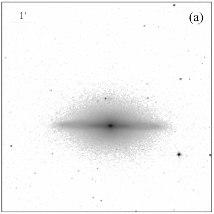
Figure 2: (a) 2MASS K-band image and (b) ACIS-S count image of NGC4594 in the 0.3-7 keV band. Detected X-ray sources are marked with circles of twice the $90\%$ EER. Sources identified as globular clusters, stars, and central nucleus (all marked with $\times$) are not included in the number-flux relation analysis (§4).

Various source detection and analysis schemes (wavelet, sliding-box, and maximum likelihood centroid fitting) have been used in previous studies (e.g., Freeman et al. 2002; Harnden et al. 1984; Cruddace et al. 1988). Applications of these schemes to Chandra imaging data have been described in Wang et al. (2003; 2004). To detect a source is to find a significant count number deviation from the expected statistical background fluctuation: the total count number $n_{c}$ within a certain detection aperture is compared with the expected contribution from the background $n_{b}$ (e.g., Fig. 3a), accounting for the statistical fluctuation. $n_{b}$ is typically estimated from the diffuse X-ray intensity in the region surrounding the detection aperture. Specifically, we first remove source candidates identified in the wavelet detection with a reduced threshold ($S/N\sim 2$) and then smooth the remaining image with a Gaussian kernel adjusted adaptively to achieve a spatially uniform count-to-noise ratio of $\sim 10$. The exposure correction for the intensity calculation accounts for such effects as the effective area variation, bad pixel/column removal, and CCD gaps. The resultant background intensity image is not sensitive to the exact source-removal threshold and smoothing method. The image, multiplied by the exposure map, gives the background count image (e.g., Fig. 3a), from which $n_{b}$ can be obtained within the corresponding detection aperture. The selected intensity-to-noise ratio in the smoothing is large enough so that the uncertainty in the background intensity estimate is small and may thus be neglected. The application of such a background map in a source search is sometimes called “the map detect algorithm”, which is well-defined for a statistical analysis of the source detection.

The significance of a count deviation above the background contribution $n_{b}$ can be characterized by the false detection probability $P$ defined as

$$P=1-\sum_{n=0}^{n_{c}-1}{n_{b}^{n}\over n!}e^{-n_{b}}.$$ (1)

If $P<P_{th}$, a preset threshold, one may declare a positive source detection. This single threshold is normally sufficient, except for the situation in which $n_{b}$ is extremely small (e.g., in regions partially covered by CCD gaps due to the telescope dithering; Fig. 1). Then an additional condition needs to be imposed for a meaningful detection (see further discussion in §3). The probability $P$, however, is for a single comparison only. In a typical blind search for sources, an entire X-ray image is scanned, invoking many statistically independent comparisons. Therefore, the false detection probability in such a search is much greater than $P$ and depends on both the detection aperture and the size of the image as well as the choice of the threshold $P_{th}$. For example, searching in count images simulated by adding Poisson noises in the background image shown in Fig. 3a yields an average of $\sim 0.05$ and 0.6 fake detections for $P_{th}=10^{-6}$ and $10^{-5}$.

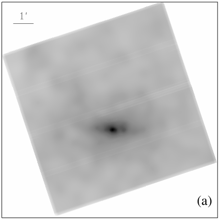
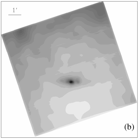
Figure 3: (a) Smoothed background map of the count image as presented in Fig. 2b. The gray-scale is in the range from 0.01 (white) to 9.0 (black). (b) Source detection threshold map for $P_{th}=10^{-6}$, showing the minimum required number of net source counts (in the range of 4 – 40) within the position-dependent source-detection aperture and above the background as shown in (a).

Figure 4: Count rates of the sources detected in the 0.3-7 keV band versus their off-axis angles in the ACIS-S observation of NGC 4594. The curves illustrate the detection thresholds ($S_{min,k}$): The upper curve is calculated via an azimuthal average, whereas the lower curve is obtained by choosing the lowest value in each concentric annulus around the aiming point of the observation. A similar plot for the Abell 2125 field is presented in Wang et al. (2004),

For a detected source, one may estimate its count rate, $S=n_{s}/(\eta t)$, where $n_{s}=n_{c}-n_{b}$, $t$, and $\eta$ are respectively the net number of source counts, the effective exposure time, and the corresponding energy-encircled fraction of the detection aperture. The count rate can be easily converted into an energy flux if an X-ray spectrum is assumed. Thus the terms, count rate and energy flux, are mostly interchangeable in the present work. The count rate threshold is $S_{min,k}=n_{s,min,k}/(\eta t_{k})$, where $n_{s,min}$ is the minimum number of source counts required for a positive detection. $S_{min,k}$ (or $n_{s,min}$; e.g., Fig. 3b) generally decreases with increasing off-axis angle, chiefly because of increasing PSF size (e.g., Figs. 1 and 2b; Jerius et al. 2000) and because of the decrease in the effective exposure (due to telescope vignetting). In the ACIS-S observation of NGC 4595 (Figs. 2 and 3), for example, the detection sensitivity is the highest at the aiming point (close to the axis of the telescope), which is about 2^′ southwest of the galaxy’s center (Fig. 3b). The sensitivity is substantially lower in the central region of the galaxy (Fig. 3b), because of the high diffuse X-ray background (Fig. 3a). The sensitivity is also low at large off-axis angles primarily due to relatively large PSF sizes, especially near the northeastern CCD boundaries (Fig. 3b). Fig. 4 presents the detected source count rates, compared with our calculated source detection thresholds.

The count rate, or flux, of a detected source represents only a single realization of the intrinsic source flux in the observation with limited counting statistics and is therefore subject to the Eddington bias.

3 Maximum Likelihood Correction for the Eddington Bias

Here we follow the approach described by Hogg & Turner (1998) but assume the Poissonian counting statistics. The likelihood that a source with an intrinsic count rate $S$ is observed to have a count rate $S_{o}$ is (see also Schmitt & Maccacaro 1986)

$$p(S_{o}|S)={(n_{s}+n_{b})^{n_{c}}\over n_{c}!}e^{-(n_{s}+n_{b})}.$$ (2)

Figure 5: The dependence of the ML flux to the observed flux ratio on $\beta={\alpha\over n_{s}}$ and $\gamma={\alpha\over n_{b}}$. The minimum $S_{ML}/S_{o}$ as a function of $\beta$ is represented by the thick curve, whereas other curves from the left to the right are for $\gamma=$ 0.01, 0.03, 0.1, 0.3, 1, 3, and 10.

The likelihood $p(S|S_{o})$ for a true count rate $S$, given that this source is observed to have a count rate $S_{o}$, is related to $p(S_{o}|S)$ by Bayes’s theorem:

$$p(S|S_{o})\propto p(S_{o}|S)f(S),$$ (3)

where $f(S)$ is the underlying intrinsic number-flux relation in the count rate interval from $S$ to $S+dS$. If the count rate measurement were unbiased, the peak in the likelihood function $p(S|S_{o})$ would be at $S/S_{o}=1$. Because of the Eddington bias, however, $S_{o}$ is statistically greater than $S$. Over a relatively small range of $S$, considered here for the bias correction, it is generally a good approximation to assume $f(S)\propto S^{-\alpha}$, where the exponent $\alpha$ is a constant and is typically around 5/2 (the so-called Euclidean slope). We take the derivative of $p(S|S_{o})$ to find its ML peak position $S_{ML}$, which leads to

$${S_{ML}\over S_{o}}={1\over 2}(1-\beta)\Bigl{\{}1+\Bigl{[}1-{4\beta^{2}\over\gamma(1-\beta)^{2}}\Bigr{]}^{1/2}\Bigr{\}},$$ (4)

where $\beta={\alpha\over n_{s}}$ and $\gamma={\alpha\over n_{b}}$. Fig. 5 illustrates the dependence of the ratio ${S_{ML}\over S_{o}}$ on these two parameters; e.g., for a fixed $\gamma$ the ratio decreases with increasing $\beta$. Evidently, the existence of the ML solution requires

$$\beta\leq\gamma^{1/2}/(2+\gamma^{1/2})$$ (5)

or

$$n_{s}\geq\alpha+(4n_{b}\alpha)^{1/2}.$$ (6)

If $\alpha=5/2$,

$$n_{s}\geq 2.5+(10n_{b})^{1/2}.$$ (7)

For example, $n_{s}$ needs to be $\gtrsim 6$, 4, or 3 for $n_{b}\sim 1$, 0.1, or 0.01 (corresponding to log$(P)=-3.2$, $-5.4$, or $-6.8$; see Eq. 1). We force this condition to be satisfied for a positive source detection, in addition to $P<P_{th}$ (§2). Otherwise, a detection with $n_{s}=1$ might be claimed as a source if $n_{b}$ is small enough (see Eq. 1), which could occur especially at edges of CCDs. The largest ML correction, or the smallest ratio ${S_{ML}\over S_{o}}$, is (see also Fig. 5)

$${S_{ML}\over S_{o}}={1\over 2}(1-\beta).$$ (8)

If $\beta\ll 1$ (i.e., $n_{s}\gg\alpha$), the solution (4) then becomes

$${S_{ML}\over S_{o}}={1\over 2}\Bigl{\{}1+\Bigl{[}1-{4\alpha\over(n_{s}/n_{b}^{1/2})^{2}}\Bigr{]}^{1/2}\Bigr{\}}.$$ (9)

This solution has the same appearance as the one derived by Hogg & Turner (1998) based on an assumed Gaussian error distribution. But $n_{s}/n_{b}^{1/2}$ here is the signal-to-background noise ratio, instead of the signal-to-noise ratio $S_{o}/\sigma$, where $\sigma$ is the Gaussian dispersion of $S_{o}$ and is assumed to be a constant (Hogg & Turner 1998). In X-ray astronomy, at least, the uncertainty in $S_{o}$ depends on $S_{o}$ itself, even when the Poissonian error distribution asymptotically approaches the Gaussian distribution for large $n_{s}$ and $n_{b}$. Furthermore, the signal-to-background noise ratio is always substantially greater than the signal-to-noise ratio $n_{s}/(n_{s}+n_{b})^{1/2}$ for the same $n_{s}$. Therefore, adopting the Poissonian error distribution, which is appropriate for the X-ray counting statistics, we can apply the ML correction to individual sources detected with only a few counts, as long as Eq. 7 is satisfied.

4 Analysis of the Number-Flux Relation

The goal of this analysis is to constrain the intrinsic (model) distribution $f(S)$ over a broad range of $S$, based on an observed number-flux distribution. Integrating Eq. (3) with a proper normalization included gives the expected number of sources in the $S_{o}$ to $S_{o}+dS_{o}$ interval

$$N(S_{o})=\int_{0}^{\infty}R(S_{o},S)f(S)dS,$$ (10)

where $R(S_{o},S)$ is the probability that a source with an intrinsic count rate $S$ is expected to have a detected count rate in the interval. The above $N(S_{o})$ can be used directly in a ML analysis of the observed source number-flux distribution to constrain model parameters in $f(S)$.

However, it is often convenient to convert the above equation into a discrete expression with $S$ and $S_{o}$ divided into channels $I$ and $J$ of small count rate widths, $\Delta_{I}=S_{I}^{u}-S_{I}^{l}$ and $\Delta_{J}=S_{J}^{u}-S_{J}^{l}$, where $l$ and $u$ denote the lower and upper count rate boundaries of the channels. We define the channels evenly on the logarithmic scale of source count rate. The overall spans of the channels should be large enough to cover the count rate range involved. For example, we choose the lowest $I$ channel to be a factor of 10 less than the lowest flux threshold of the source detection. By integrating over each channel $J$ on both sides of Eq. 10, we get

$$N(J)=\sum_{I}R(J,I)f(I)\Delta_{I},$$ (11)

where

$$f(I)=\int_{S_{I}^{l}}^{S_{I}^{u}}f(S)dS/\Delta_{I}$$ (12)

and the redistribution matrix

$$R(J,I)={\int_{S_{I}^{l}}^{S_{I}^{u}}R(J,S)f(S)dS\over\int_{S_{I}^{l}}^{S_{I}^{u}}f(S)dS},$$ (13)

in which $R(J,S)=\int_{S_{J}^{l}}^{S_{J}^{u}}R(S_{o},S)dS_{o}$. In practice, $\Delta_{I}$ can be chosen to be small enough so that

$$R(J,I)\approx R(J,S_{I}),$$ (14)

where $S_{I}$ may be defined as $S_{I}=(S_{l}S_{u})^{1/2}$.

As discussed in §3, the redistribution matrix is basically the Poisson probability distribution, although an average is required over the field from which the sources are detected. This step is similar to the construction of a weighted instrument redistribution function for the spectral analysis of a diffuse X-ray feature. In the present case, the average is needed because the source detection sensitivity varies across the field. The matrix defined at each pixel $k$ can be expressed as

$$R_{k}(J,S_{I})=\left\{\begin{array}[]{ll}0&\textrm{if $S_{J}^{u}\leq S_{min,k}$}\\ Q_{k}(<S_{J}^{u},S_{I})-Q_{k}(<S_{J}^{l},S_{I})&\textrm{if $S_{J}^{l}\geq S_{min,k}$}\\ Q_{k}(<S_{J}^{u},S_{I})-Q_{k}(<S_{min,k},S_{I})&\textrm{if $S_{J}^{l}<S_{min,k}<S_{J}^{u}$}\end{array}\right.$$ (15)

where $Q_{k}$ is the accumulated Poisson probability (see also Eq. 2). For example,

$$Q_{k}(<S_{J}^{u},S_{I})=\sum_{n=0}^{n_{max}}{(\eta t_{k}S_{I}+n_{b,k})^{n}\over n!}e^{-(\eta t_{k}S_{I}+n_{b,k})},$$ (16)

where $n_{max}$ is the largest integer that is smaller than $\eta t_{k}S_{J}^{u}+n_{b,k}$. When the expected value of $\eta t_{k}S_{I}+n_{b,k}$ is large, $Q_{k}$ can be replaced by the standard error function of a Gaussian distribution. The calculation does not need to be done for all $J$ channels, as long as the range included covers essentially all the redistribution probability; a 4$\sigma$ range around each $S_{I}$ is calculated in our applications. XSPEC, for example, allows for a redistribution matrix with a variable $J$ channel dimension. The redistribution matrix averaged over all pixels is then

$$R(J,I)=\sum_{k=1}^{N_{p}}R_{k}(J,I)\xi_{k},$$ (17)

and

$$\sum_{k=1}^{N_{p}}\xi_{k}=1,$$ (18)

where $\xi_{k}$ is the intrinsic probability for a source to appear at the $k$th pixel and may be inferred from their empirical spatial distribution, from a model, and/or from an image in another wavelength band (e.g., optical). For example, to estimate the total number of background sources in a field $N_{s,b}$, we can assume a uniform probability distribution (i.e., $\xi_{k}=1/N_{p}$). On the other hand, we may assume that a source population of galaxy follows its near-infrared light (e.g., Fig. 2a) with an intensity $I_{k}$ at pixel $k$. Under these assumptions, we have

$$\xi_{k}={N_{s,b}\over N_{s}N_{p}}+(1-{N_{s,b}\over N_{s}}){I_{k}\over\sum_{k=1}^{N_{p}}I_{k}},$$ (19)

where $N_{s}$ is the total number of detected sources, background plus galactic.

The above defined $R(J,I)$ accounts for both the detection threshold variation and the flux redistribution of the sources. Fig. 6 shows an example of the redistribution matrix. As expected, the Eddington bias causes a systematic shift of the probability distribution peak (for a fixed $S$) to the right of $S_{o}=S$, apparent for $S\lesssim 10^{-3}{\rm~{}counts~{}s^{-1}}$. The dispersion in $S_{o}$ also increases with decreasing $S$. Effects due to the discreteness of the Poissonian distribution are apparent at low $S_{o}$ values. Fig. 7 illustrates these effects for three representative $S$ values. Furthermore, the sum of $R(J,I)$ over $J$ channels gives the average detection probability as a function of intrinsic source count rate (e.g., Fig. 8).

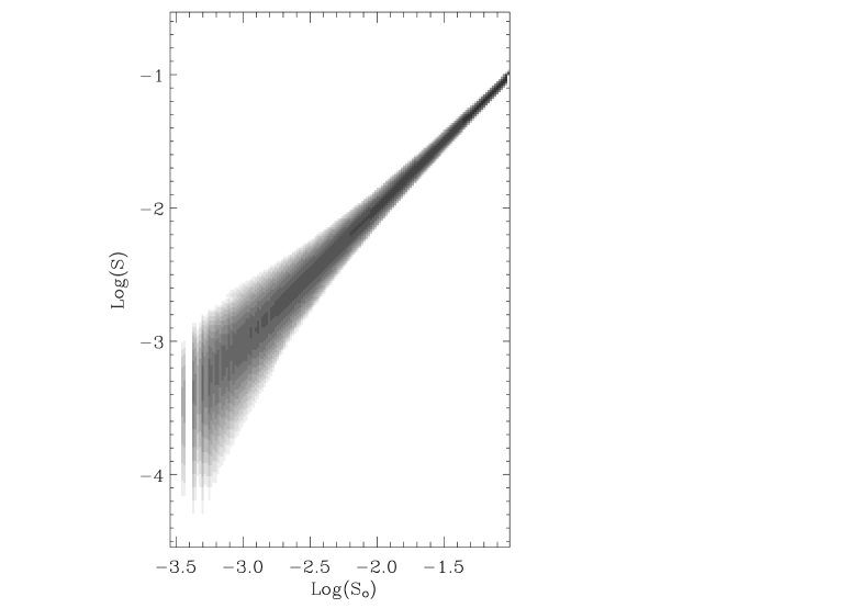
Figure 6: Source count rate distribution matrix in the 0.3-7 keV band for the NGC 4594 observation (see also Figs. 2-3; see also §5). The probability is scaled from $1\times 10^{-5}$ (white) to 0.4 (black), logarithmically. Both $S$ and $S_{o}$ are in units of ${\rm~{}counts~{}s^{-1}}$.

Figure 7: Illustration of the average source flux redistribution probability in the NGC 4594 observation. The vertical straight lines mark the selected intrinsic source fluxes ($S$), whereas the curves represent the probability distribution of the corresponding flux ($S_{o}$). Notice that the solid line marks an $S$ value that is below the lowest detection threshold of $\sim 3\times 10^{-4}{\rm~{}counts~{}s^{-1}}$.

$R(J,I)$, together with the count rate boundaries of the $I$ and $J$ channels (all included in a standard fits file), can be imported into XSPEC. The only other file required is the histogram of the detected sources in the $J$ channels. All other calculations, such as the binning of the model distribution, are performed automatically within XSPEC, which also allows for using $\chi^{2}$ or Cash’s C-statistic in the model-fitting and for estimating model parameter uncertainties.

The model distribution $f(S)$ can essentially be in any form, e.g., an additive and/or multiplicative combination of various components. Different components may have different count rate-to-energy flux conversions, which depend on the line-of-sight absorption/scattering as well as the assumed intrinsic source spectra. Allowing for this flexibility is the primary reason for us to use count rates, instead of energy fluxes here. If a single conversion (i.e., a single incident spectrum) is assumed for all sources, expressing the procedure described above in terms of energy fluxes is trivial.

Figure 8: Average detection probability of a source as a function of its intrinsic count rate in the NGC 4594 observation.

5 Applications

While the ML Eddington bias estimate for individual sources is straight forward, we concentrate on the application of the source flux redistribution matrix. This procedure follows the standard data calibration, exposure map construction, source detection, and background image generation (e.g., Wang et al. 2003, 2004; see also Figs. 1-3). We adopt $P_{th}=10^{-6}$. From the ACIS-I observation of Abell 2125, we detect 81, 48, and 93 sources in the 0.5-2, 2-8, and 0.5-8 keV bands, respectively. From the ACIS-S observation of NGC 4594, 80, 65, and 112 sources are detected in the 0.3-1.5, 1.5-7, and 0.3-7 keV bands, respectively. After removing duplicates (spatial coincidences) in the detections, we find a total of 99 and 115 unique sources in the Abell 2125 and NGC 4594 fields (Figs. 1 and 2b). We then apply the procedure described in §4 to generate the required flux redistribution matrix $R(J,I)$ for each source detection band (e.g., Fig. 6), which can then be used to study the number-flux relations in the fields.

5.1 Contribution from Interlopers

In a typical Chandra imaging observation, a considerable fraction, if not most, of the detected sources are interlopers. In a high Galactic latitude field, interlopers are typically background AGNs, plus a small number of foreground stars. The number-flux relation of such interlopers has been characterized in various X-ray surveys, including the Chandra ACIS-I deep surveys (Moretti et al. 2003 and references therein). In almost all recent work, this characterization is done separately in the 0.5-2 keV and 2-10 keV bands. The source populations detected in these two bands only partially overlap: Sources with steep X-ray spectra preferentially appear in the 0.5-2 keV band, whereas highly-absorbed ones appear in the 2-10 keV band. In general, Chandra is much more sensitive to sources in the former band than in the latter band. Therefore, we focus on the accumulated number-flux relation in the 0.5-2 keV band, which can be modeled as:

$$N(>S)=N_{0}\Bigl{[}{(2\times 10^{-15})^{\alpha_{1}}\over S^{\alpha_{1}}+S_{0}^{\alpha_{1}-\alpha 2}S^{\alpha_{2}}}\Bigr{]},$$ (20)

where $N_{0}=6150{\rm~{}sources~{}deg^{-2}}$, $\alpha_{1}=1.82$, $\alpha_{2}=0.60$, and $S_{0}=1.48\times 10^{-14}{\rm~{}erg~{}s^{-1}~{}cm^{-2}}$ (Moretti et al. 2003). We have implemented this model in XSPEC, which automatically computes $f(I)=[N(>S_{I}^{l})-N(>S_{I}^{u})]A$, where $A$ in units of deg² is the FoV of the observation in consideration. By convolving $f(I)$ with $R(J,I)$, we may predict the number-flux relation of the interlopers (Eq. 11).

Figure 9: The on-axis count rate ratio in different bands versus X-ray-absorbing gas column density for a representative power-law models. (a) The ACIS-I ratios: 0.5-8 keV to 0.5-2 keV (thick curves) and 0.5-8 keV to 2-8 keV (thin curves). (b) The ratios: ACIS-S 0.3-7 keV to ACIS-I 0.5-2 keV (thick curves) and ACIS-S 0.3-7 keV to ACIS-I 2-8 keV (thin curves). The three styles of the curves correspond to photon index choices: 1.4 (solid), 1.7 (dotted), and 2 (dashed).

However, caution must be exercised in using Eq. 20. The energy flux $S$ specifically depends on the count rate-to-energy flux conversion that assumes a power law with a photon index of 1.4 plus a foreground absorption of $1.6\times 10^{20}{\rm~{}cm^{-2}}$. Indeed, the power law is a good description of the overall spectral shape of the extragalactic X-ray background, which is now believed to be a composite of mostly AGNs. But, X-ray spectral properties do vary greatly from one source to another. Statistically, the average X-ray spectrum of AGNs tends to become flatter with decreasing flux, apparently due to an increasing population of highly-absorbed AGNs. Unfortunately, such spectral variations are not yet well quantified and thus cannot be incorporated easily into the calculation of the count rate-to-energy flux conversion. Obviously, a deviation from the assumed source spectrum could cause errors. To minimize this effect, we convert the energy flux in the model back into the count rate in the 0.5-2 keV band of an ACIS-I observation, using the same assumed power law, but with the foreground absorption appropriate to a particular field. In the case of the Abell 2125 observation, for example, we use $N_{H}=3\times 10^{20}{\rm~{}cm^{-2}}$ to derive the conversion as $4.5\times 10^{-12}$ ${\rm~{}(erg~{}cm^{-2}~{}s^{-1}})/({\rm counts~{}s^{-1}})$, which leads to a predicted number-flux relation of the interlopers, as is shown in Wang et al (2004).

To construct the observed number-flux relation, we exclude the 10 sources that have been found to be in positional coincidence with Abell 2125 complex member galaxies (Wang et al. 2004). These members are all detected in both 0.5-2 keV and 0.5-8 keV bands. We construct the observed relation in the 0.5-2 keV band by grouping the remaining 71 sources to have a minimum number of $\sim 8$ sources per count rate bin. A direct comparison between the observed and predicted relations (not a fit) gives a C-statistic value of 6.9 for a total of 9 bins. The probability to have a C-statistic less than this value is 38%, according to Monte-Carlo simulations in XSPEC. Therefore, the two relations are statistically consistent with each other.

A source number-flux relation comparison may also be made for detections in other bands. This comparison is particularly desirable for the ACIS-I 0.5-8 keV band, in which the source detection is typically most sensitive. However, we are not aware of any number-flux relation constructed recently for interlopers in this band. Indirectly, one may still use Eq. 20 by converting the flux to the count rate in the 0.5-8 keV band. This approach implicitly uses the ratio of the 0.5-8 keV to 0.5-2 keV count rates, which depends on an assumed source spectrum (Fig. 9a). For a typical AGN spectrum with a power-law photon index between 1.4-2 and an absorption smaller than $\sim 10^{22}{\rm~{}cm^{-2}}$, a good approximation for the ratio is 1.3. With this approximation, the comparison between the observed and expected number-flux relations of the Abell 2125 sources in the 0.5-8 keV band gives a C-statistic value of 18.4 for 10 bins, which may be rejected with a confidence of $\sim 94\%$. The predicted number of sources is 75, compared to 83 actual detections (the complex members are excluded). This difference is partly due to the expected presence of relatively hard X-ray sources, which are not detected in the 0.5-2 keV band and are thus not included in the number-flux relation extrapolated from the same band. Unfortunately, the poor number statistics of such sources detected in the field prevents us from placing a tight constraint on their population. In addition, one also expects an intrinsic cosmic variance in the source number density from one field to another, typically $\gtrsim 6\%$, depending on the FoV, energy band, and source detection limit of observations (see Yang et al. 2003 and references therein). Therefore, even in a relatively deep exposure such as the Abell 2125 observation, the number of interlopers cannot be predicted accurately.

The relative uncertainty in the number of interlopers becomes even greater for an ACIS-S observation, because of both its small FoV (at least for the BI CCD #7 chip alone) and its different energy response from the FI CCDs of the ACIS-I. There is not yet a number-flux relation constructed for ACIS-S detected interlopers. Nevertheless, an approximate estimate is often required. One may use an approach similar to the one described above for the ACIS-I 0.5-8 keV band. By adopting a ratio of the ACIS-S 0.3-7 keV to ACIS-I 0.5-2 keV count rates as $\sim 2.2$ (Fig. 9b), for example, we find that the expected number of interlopers is $N_{s,b}\sim 16$ in the NGC 4594 observation, compared with 112 sources detected in the 0.3-7 keV band. Although the relative uncertainty in the expected number of interlopers is statistically large, the bulk of the detected sources are clearly associated with the galaxy.

5.2 Number-Flux Relation of X-ray Sources in NGC 4594

To facilitate a comparison with the analysis by Di Stefano et al. (2003), we also exclude sources that have been identified as foreground stars as well as the nucleus and globular clusters of NGC 4594. Fig. 10 presents the number-flux relation for the remaining $N_{s}=90$ sources detected in the 0.3-7 keV band. We calculate the re-distribution matrix, by using Eq. 19 with $N_{s,b}=16$ as estimated above and the 2MASS K-band image (Fig. 2a) as the galactic source probability distribution. Foreground stars in the image are removed approximately with a 9$\times$9 pixel median filter (pixel size = 1$\farcs$5). The predicted interloper contribution is small and is thus fixed in the subsequent number-flux analysis. First, we model the galactic component, using a single power law and get the best fit as

$${\rm Log}[N(S)]=-1.6_{-0.39}^{+0.38}-2.1_{-0.12}^{+0.14}{\rm Log}(S)$$ (21)

(all error bars are at the $1\sigma$ confidence level); the C-statistic value 17.0 for 9 degrees of freedom can only be rejected statistically at a confidence $\sim 92\%$. Considering all the additional uncertainties that are not included in the analysis (e.g., interloper subtraction errors), we consider the single power law fit is still reasonably acceptable.

Next, we fit the observed number-flux relation with a broken power law (see also Di Stefano et al. 2003),

$$\left({dN\over dS}\right)=N_{b}\left({S\over S_{b}}\right)^{-\Gamma},$$ (22)

where $\Gamma=\Gamma_{1}$ for $S\leq S_{b}$ and $\Gamma=\Gamma_{2}$ for $S>S_{b}$. With an addition of only two more model parameters than in the single power law, this model fit gives a C-statistic value of 8.87, which is satisfactory (Fig. 10). The best-fit parameters are $N_{b}=1.7\times 10^{4}{\rm~{}sources/(counts~{}s^{-1}})$, $S_{b}=2.1_{-0.7}^{+1.1}\times 10^{-3}$, $\Gamma_{1}=1.4_{-0.3}^{+0.3}$, $\Gamma_{2}=4.6_{-1.2}^{+2.7}$. Fig. 11 presents the confidence contours, $\Gamma_{1}$ vs. $\Gamma_{2}$.

Figure 10: Observed differential number-flux relation of the sources detected in the 0.3-7 keV band, compared with the best-fit broken power-law model (dash-dotted histogram) plus the expected interloper contribution (dashed) in the field of NGC 4594. The combination of the two model components is represented by the solid histogram.

Figure 11: The 68%, 90%, and 99% confidence contours of the broken power law indexes from the best fit shown in Fig. 10.

In comparison, the analysis by Di Stefano et al. (2003) suggests $\Gamma_{1}=0.74_{-1.04}^{+0.84}$, $\Gamma_{2}=2.58_{-0.28}^{+0.35}$, and a luminosity break at $9_{-1.6}^{+2.0}\times 10^{37}{\rm~{}erg~{}s^{-1}}$, corresponding to a count rate break $S_{b}\sim 1.8_{-0.32}^{+0.40}\times 10^{-3}{\rm~{}counts~{}s^{-1}}$, assuming a power law spectrum of photon index 2 and an absorption of $N_{H}=5\times 10^{20}{\rm~{}cm^{-2}}$ (Di Stefano et al. 2003). While these parameters are marginally consistent with those obtained from our analysis, their constraints on $S_{b}$ seem to be considerably tighter than ours.

This difference is probably largely due to the simplification made in the analysis by Di Stefano et al. (2003). Their analysis ignored both the background source contribution and the Eddington bias and assumed a single source-detection threshold of $4.5\times 10^{37}{\rm~{}erg~{}s^{-1}}$, or a count rate of $9\times 10^{-4}{\rm~{}counts~{}s^{-1}}$, inferred from the peak at $S/N\sim 3.2$ in a number-$S/N$ histogram of the detected sources. However, Fig. 8 shows that the average detection probability is still only $\sim 80\%$ at this count rate. A detection probability $\gtrsim 95\%$, for example, requires a source count rate $\gtrsim 1.4\times 10^{-3}{\rm~{}counts~{}s^{-1}}$. Clearly, part of the turn-over in the observed number-flux relation at $S_{b}$ (Fig. 10) is due to the flux-dependent source detection threshold, which should be accounted for in the modeling. Setting a threshold at a higher count rate should have reduced this flux dependence. But more than half of the sources would then be excluded in the analysis.

Of course, the flux-dependence of the threshold is a result of the detection sensitivity variation across the field. The variation is even greater for an ACIS-I observation, because of the larger off-axis FoV. Therefore, a proper correction for the flux-dependent threshold is essential to the analysis of the source number-flux relation, especially to the full utilization of detected sources.

6 Summary

We have examined the detection threshold and the Eddington bias in flux measurements for sources identified with limited Poisson counting statistics. Our main results are as follows:

• We have derived a ML correction for the flux measurement bias, based on a Poissonian error distribution. This correction can be applied to individual sources detected with very limited counting statistics. The condition for the presence of the ML correction (Eq. 7) should be required for a source detection, in addition to the probability threshold.

• The source detection threshold varies strongly with position, especially with the off-axis angle. A flux-dependent correction for this threshold variation is essential to the statistical analysis of detected sources.

• We have developed a simple procedure to calculate the flux redistribution matrix, based on the exposure and diffuse background maps obtained directly from an observation. The matrix inherently accounts for both the source detection threshold variation and the Eddington bias and can be imported into a software package such as XSPEC so that the number-flux relation can be analyzed as if it were an X-ray spectrum.

• We have applied the procedure to a deep ACIS-I observation of the Abell 2125 complex. With 10 identified complex members excluded, the remaining X-ray sources show a number-flux relation that is consistent with the expected interlopers of the field.

• We have also analyzed the number-flux relation of X-ray sources detected in an ACIS-S observation of NGC 4594. While the contribution from the expected interlopers is shown to be small, we have characterized the number-flux relation of the galactic sources, using either a power law or a broken power law. The latter model gives a considerably better characterization than the former.

The techniques described in this paper can be easily implemented; an IDL procedure for generating the flux-redistribution matrix, for example, can be obtained from the author.

References

- (1) Arnaud, K. A. 1996, in Astronomical Data Analysis Software and Systems V (ASP Conf. Series volume 101), eds. Jacoby G. and Barnes J., p17
- (2) Cruddace, R. G., Hasinger, G. R., & Schmitt, J. H. 1988, in Astronomy from Large Databases, ed. F. Murtagh & A. Heck (München: ESO), 177
- (3) Di Stefano, R., et al. 2003, ApJ, 599, 1067
- (4) Eddington, A. S. 1940, MNRAS, 100, 354
- (5) Freeman, P. E., Kashyap, V., Rosner, R., & Lamb, D. Q. 2002, ApJS, 138, 185
- (6) Hasinger, G., et al. 1993, A&A, 275, 1
- (7) Harnden, F. R., Jr., Fabricant, D. G., Harris, D. E., & Schwarz, J. 1984, Smithsonian Ap. Obs. Spec. Repr., No. 393
- (8) Hogg, D. W., & Turner, E. L. 1998, PASP, 110, 727
- (9) Jerius, D., et al. 2000, SPIE, 4012, 17
- (10) Kenter, A. T., & Murray, S. S. 2003, ApJ, 584, 1016
- (11) Moretti, A., Campana, S., Lazzati, D., & Tagliaferri, G. 2003, A&A, 588, 696
- (12) Murdoch, H. S., Crawford, D. F., & Jauncey, D. L. 1973, ApJ, 183, 1
- (13) Schmitt, J. H. M. M., & Maccacaro, T. 1986, ApJ, 310, 334
- (14) Wang, Q. D., Chaves, T., & Irwin, J. 2003, ApJ, 598, 969
- (15) Wang, Q. D., Owen, F., & Ledlow, M. 2004, ApJ, 611, in press
- (16) Yang, Y., et al. 2003, ApJ, 585, 85