LMC Self-lensing from a new perspective

We present a new analysis on the issue of the location of the observed microlensing events in direction of the Large Magellanic Cloud (LMC). This is carried out starting from a recently drawn coherent picture of the geometrical structure and dynamics of the LMC disk and by considering different configurations for the LMC bar. In this framework it clearly emerges that the spatial distribution of the events observed so far shows a near–far asymmetry. This turns out to be compatible with the optical depth calculated for the LMC halo objects. In this perspective, our main conclusion, supported by a statistical analysis on the outcome of an evaluation of the microlensing rate, is that self lensing can not account for all the observed events. Finally we propose a general inequality to calculate quickly an upper limit to the optical depth along a line of view through the LMC center.

1 Introduction

The microlensing surveys towards the Large Magellanic Cloud (LMC) (Alcock et al. 2000a; Lasserre et al. 2000) have demonstrated the existence of compact objects that act as gravitational lenses somewhere between us and the LMC. In some cases the distance and the mass of the lenses have been determined, thanks to the proper motion of the lens observed by the Hubble Space Telescope (HST) (Alcock et al. 2001a; Gould 2004; Drake et al. 2004) or to the additional information carried by binary systems (Alcock et al. 2000b, 2001b). However, these are special cases since for most events only the duration and the position on the sky plane have been measured. These information are not enough to establish definitively if the detected events are really caused by white dwarfs or MACHOs in the halo of the Milky Way (MW), or are due to stars or MACHOs within the LMC itself.

The survey of the MACHO team indicates a most probable Galactic halo fraction of 20%, with limits of 5% to 50% at the 95% confidence level, assuming that all the events are due to halo lenses. The preferred value for the lens mass is $\sim$ 0.4 M_☉. This is consistent with the EROS survey results, that are given however as an upper limit for the Galactic halo fraction.

An interesting alternative is that of “self lensing”, where both source and lens belong to the luminous part of the LMC as suggested by Sahu (1994) and Wu (1994). However, the initial estimates of the optical depth and microlensing rate were lower than the measured one (Gould 1995; Alcock et al. 1997, 2000a). The self–lensing explanation has been further analyzed going beyond the hypothesis of a “simple” geometry for the LMC with disk and bar coplanar, so that their relative distance would enhance the optical depth and, therefore, the rate. In the model of Zhao & Evans (2000) the disk and bar stars are on two distinct planes with different inclinations, so that stars on the front plane could lens those in the plane $\approx$ 1 kpc behind. Besides the morphology, another aspect considered has been the dynamics of the luminous components within the LMC. Aubourg et al. (1999), by using a model which takes into account the correlation between the mass of the lenses in the LMC and their velocity dispersion, have been able to reproduce a self–lensing optical depth, event rate and event duration distribution compatible with the observed ones. Yet, objections to this model have been raised by different authors (Gyuk et al. 2000; Alves & Nelson 2000), especially with respect to the adopted distribution and velocity dispersion of the lensing stars, which seem to be inconsistent with the observations.

The analysis of Jetzer et al., (2002, hereafter Paper I) has shown that probably the observed events are distributed among different components (disk, spheroid and galactic halo, the LMC halo and self–lensing). This means that the lenses do not belong all to the same population and their astrophysical features can differ deeply from one another.

In this paper we address once more the question of the presence of a self–lensing component within the LMC itself. To this end a correct knowledge of the structure and dynamics of the luminous components (disk and bar) of the LMC is essential. Here we take advantage of some recent studies of the LMC disk (see Sect. 2.1), while we allow for different geometries for the still poorly known bar component, to calculate the main microlensing quantities. Moreover, with respect to Paper I, based on the moment method (de Rújula et al. 1991), we perform instead a statistical analysis starting from the differential rate of the microlensing events.

The paper is organized as follows: in Sects. 2 and 3 we discuss the LMC morphology and present the models we use to describe the spatial density of the MW halo and of the various components of the LMC. Sect. 4 is devoted to the calculation of the microlensing quantities, the optical depth and the microlensing rate, as well as to a statistical analysis of the self–lensing events. In Sect. 5 we discuss the spatial asymmetry with respect to the line of nodes of the observed microlensing events. An improved inequality for the optical depth for self lensing by a stellar disk is derived in Sect. 6. We conclude in Sect. 7 with a summary of our results.

2 Observational data

2.1 LMC Disk morphology

Recently, in a series of three interesting papers (van der Marel & Cioni 2001; van der Marel 2001; van der Marel et al. 2002), a new coherent picture of the geometrical structure and dynamics of the LMC disk has been given. By using the data from two near-infrared surveys, DENIS (Cioni et al. 2000) and 2MASS (Cutri et al. 2000) stellar catalogs, the LMC geometry has been constrained by carefully studying the star count map and the characteristic apparent magnitudes of Asymptotic Giant Branch (AGB) and Red Giant Branches (RGB) stars. The results have been further improved by a detailed and sophisticated study of the LMC line-of-sight velocity field, coupled with a multi-parameter fit on the available velocities of 1041 carbon stars. A basic assumption is that the carbon star population is representative for the bulk of the LMC stars.

The first important conclusion is that the intrinsic shape of the LMC disk is not circular, as assumed before, but elliptical, with an intrinsic ellipticity $\epsilon^{\prime\prime}=0.312\pm 0.007$. The inclination angle of the LMC disk plane is $i=34.7^{\circ}\pm 6^{\circ}$ and the line-of-nodes position angle is $\Theta=129.9^{\circ}\pm 6^{\circ}$. This value is quite different from the LMC disk major axis position angle, $\mathrm{PA}_{\mathrm{maj}}=189.3^{\circ}\pm 1.4^{\circ}$, corresponding to a position angle $\Phi=202.7^{\circ}\pm 1.9^{\circ}$ when measured in the equatorial plane of the LMC disk, starting from the axis pointing towards the North. The radial number density profile along the major axis follows, to lowest order, an exponential profile with an intrinsic scale length equal to 1.54 kpc.

A second important conclusion is that the center of mass (CM) of the carbon stars is consistent with the center of the bar and with the center of the outer isophotes of the LMC. As a consequence, the idea of using the distribution of neutral gas as good tracer for the disk stars, that leads to an incorrect LMC model, must be abandoned. The obtained values of the right ascension and declination of the CM, given in J$2000$, are $\alpha_{\mathrm{CM}}=5^{\mathrm{h}}\,27.6^{\mathrm{m}}\pm 3.9^{\mathrm{m}}$, $\delta_{\mathrm{CM}}=-\,69.87^{\circ}\pm 0.41^{\circ}$. The weighted mean of the rotation velocity in the range 4–8.9 kpc, where the rotation curve is approximately flat, is $V=49.8\pm 15.9$ km/s, about $40\%$ lower than the previously inferred and accepted value. Taking into account the asymmetric drift effect, the circular velocity has been corrected and estimated to be equal to $V_{\mathrm{circ}}=64.8\pm 15.9$ $\mathrm{km}\,\mathrm{s}^{-1}$. The line-of-sight velocity dispersion has an average value $\sigma=20.2\pm 0.5$ km $\mathrm{s}^{-1}$, and is little dependent on the radius. The rate of inclination change is ${\mathrm{d}i\over\mathrm{d}t}=-\,0.37\pm 0.22$ $\mathrm{mas}\,\mathrm{yr}^{-1}$, a value similar to that determined from N-body simulations by Weinberg (2000), which predicts the LMC disk precession and nutation to be due to tidal torques generated by our Galaxy.

A third important conclusion is that the LMC disk has a considerable vertical thickness, in agreement also with the numerical simulations of Weinberg (2000). The thickening of the LMC disk is due to the gravitational interaction with the MW. The ratio ${V\over\sigma}=2.9\pm 0.9$ is even lower than the corresponding value for the MW thick disk (${V\over\sigma}\simeq 3.9$). The LMC disk is also flared. The best fit of the observed velocity dispersion profile with isothermal disk models, whose vertical density profile is proportional to $\mathrm{sech}^{2}({z\over z_{0}})$, confirms the result found by Alves & Nelson (2000) that the scale height must increase with radius. The vertical thickening is also in agreement with the results of Olsen & Salyk (2002), who argued that the LMC contains features that extend up to 2.5 kpc out of the plane.

Let us note that recently some of these conclusions have been challenged by Nikolaev et al. (2004), whose analysis is based on a combination of the results of the MACHO collaboration on the LMC Cepheides with the $2$MASS All-Sky Release Catalog.

2.2 LMC Dark Halo

Another important conclusion of the van der Marel et al. analysis, is connected with the LMC dark halo. Comparing the LMC total mass enclosed in a sphere of $8.9$ kpc, dynamically inferred to be $(8.7\pm 4.3)\times 10^{9}\,\mathrm{M}_{\sun}$, with respect to the visible mass $M_{\mathrm{vis}}\approx 2.7\times 10^{9}\mathrm{M}_{\sun}$, and to the mass of neutral gas $\approx 0.5\times 10^{9}\mathrm{M}_{\sun}$ (Kim et al. 1998), van der Marel et al. (2002) have concluded that the LMC must be surrounded by a dark halo with a radius equal to the LMC tidal radius $r_{\mathrm{t}}=15.0\pm 4.5$ kpc, a value higher than that, $11\,\mathrm{kpc}$, estimated by Weinberg (2000). Moreover, at a distance of 5 kpc from the center of the LMC, the ratio between the tidal force and the LMC self gravitational attraction is reduced by 20%. Thus, one expects that tidal effects influence deeply the structure of the LMC halo, causing probably an elongation of it.

3 Models

We adopt the same coordinate systems and notations as in van der Marel et al. (2002). The position of any point in space is uniquely determined by the two angles, right ascension $\alpha$ and declination $\delta$, and by its distance $D$. We introduce also a cartesian coordinate system $(x,\,y,\,z)$ that has its origin $O$ in the center of the LMC, whose coordinates are $(\alpha_{0},\,\delta_{0},\,D_{0})$, with the $x$–axis antiparallel to the right ascension axis, the $y$–axis parallel to the declination axis, and the $z$–axis pointing towards the observer. To describe the internal kinematics of the galaxy it is opportune to introduce a second cartesian coordinate system $(x^{\prime},\,y^{\prime},\,z^{\prime})$ that is obtained from the system $(x,\,y,\,z)$ by a counterclockwise rotation around the $z$–axis by an angle equal to the position angle of the line of nodes $\Theta-{\frac{\pi}{2}}$, followed by a rotation around the new $x^{\prime}$–axis by an angle equal to the inclination angle of the disk plane $i$. With this definition the $(x^{\prime},\,y^{\prime})$ plane coincides with the equatorial plane of the LMC galaxy, and the $x^{\prime}$–axis is along the line of nodes.

3.1 LMC Disk

Following the new results on the LMC morphology discussed in Sect. 2, we consider an elliptical isothermal flared disk tipped by an angle $i=34.7^{\circ}\pm 6.2^{\circ}$ with respect to the sky plane, with the closest part in the north-east side. The center of the disk coincides with the center of the bar located at J2000 ($\alpha,\delta$) = ($5^{h}27.6^{m}\pm 3.9^{m},-69.87^{\circ}\pm 0.41^{\circ}$) and its distance from us is $D_{0}=50.1\pm 2.5\,\mathrm{kpc}$. Here we take a bar mass $M_{\mathrm{bar}}=1/5\,M_{\mathrm{disk}}$ (Sahu 1994; Gyuk et al. 2000), with the visible mass in disk and bar $M_{\mathrm{bar}}+M_{\mathrm{disk}}=(2.7\pm 0.6)\times 10^{9}\,\mathrm{M}_{\sun}$ (van der Marel et al. 2002).

The vertical distribution of stars in an isothermal disk is described by the $\mathrm{sech}^{2}$ function, therefore the spatial density of the disk is modelled by:

$$\rho_{\mathrm{d}}=\frac{{\cal N}\,M_{\mathrm{d}}}{4\pi\,q\,R_{\mathrm{d}}^{2}\,\zeta_{\mathrm{d}}(0)}\;\mathrm{sech}^{2}\left(\frac{\zeta}{\zeta_{\mathrm{d}}(R)}\right)e^{-{\frac{1}{R_{\mathrm{d}}}}\sqrt{\left(\frac{\xi}{q}\right)^{2}+{\eta}^{2}}}\leavevmode\nobreak\ ,$$ (1)

where $q=0.688$ is the ellipticity factor, $R_{\mathrm{d}}=1.54\,\mathrm{kpc}$ is the scale length of the exponential disk, $R$ is the radial distance from the center on the disk plane. ${\zeta_{\mathrm{d}}(R)}$ is the flaring scale height, which rises from 0.27 kpc to 1.5 kpc at a distance of 5.5 kpc from the center (van der Marel et al. 2002), and is given by

$${\zeta_{\mathrm{d}}(R)}=0.27+1.40\,\tanh\left(\frac{R}{4}\right)\leavevmode\nobreak\ .$$

${\cal N}=0.2765$ is a normalization factor that takes into account the flaring scale height.

The cartesian coordinates $(\xi,\,\eta,\,\zeta\equiv z^{\prime})$ are obtained from the system $(x^{\prime},\,y^{\prime},\,z^{\prime})$ by rotation around the $z^{\prime}$-axis by an angle equal to $(\Phi-\Theta-{\frac{\pi}{2}})$, where $\Phi$ is the position angle of the LMC disk major axis. In this way the $\xi-\eta$ plane coincides with the equatorial disk plane and the $\eta$ axis is directed along the major axis of the elliptic disk.

The velocity dispersion is a crucial parameter for the estimate of the microlensing rate. The kinematic studies of the LMC disk have shown that measurements of the velocity dispersion along the line of sight vary between roughly $6$ and $30$ km/s, according to the age of the tracers and show little variation as a function of the radius (see Gyuk et al. (2000) where a comprehensive table is given). In particular, younger populations have a smaller velocity dispersion than older ones, as in the MW. In the picture of van der Marel et al. (2002) within a distance of about 3 kpc from the center of the LMC, the line of sight velocity dispersion (evaluated for carbon stars) can be considered as constant with $\sigma_{\mathrm{d,los}}=20.2\pm 0.5$ km/s. This represents our choice for the line of sight velocity dispersion of the disk stars.

3.2 LMC Bar

An optical bar of roughly $3^{\circ}\times 1^{\circ}$ angular size stands out in the central region of the LMC. Unlike the disk, the geometry of the bar region, in particular its vertical structure, is not well constrained. Understanding how the bar is displaced with respect to the disk is one of the last information needed to complete the puzzle of the LMC morphology.

In Paper I we have described the bar by a gaussian density profile following Gyuk et al. (2000). In this paper we choose, instead, a bar spatial density that takes into account its boxy shape, as in Zhao & Evans (2000):

$$\rho_{\mathrm{b}}=\frac{2\,M_{\mathrm{b}}}{\pi^{2}\,R_{\mathrm{b}}^{2}\,\,\Xi_{\mathrm{b}}}\,e^{-\left(\frac{\Xi}{\,\Xi_{\mathrm{b}}}\right)^{2}}\,e^{-\,\frac{1}{R_{\mathrm{b}}^{4}}\left(\Upsilon^{2}+\,\zeta^{2}\right)^{2}},$$ (2)

where $\Xi_{\mathrm{b}}=1.2\,\mathrm{kpc}$ is the scale length of the bar axis, $R_{\mathrm{b}}=0.44\,\mathrm{kpc}$ is the scale height along a circular section, and the cartesian coordinates $(\Xi,\,\Upsilon,\,\zeta\equiv z^{\prime})$ are obtained from the system $(x^{\prime},\,y^{\prime},\,z^{\prime})$ by rotating around the $z^{\prime}$-axis by an angle equal to $(\Psi-\Theta)$, where $\Psi$ is the position angle of the LMC bar major axis, roughly $\simeq 120^{\circ}$ (van der Marel 2001). We fix it to $112.7^{\circ}$, so that the bar major axis $\Xi$ coincides with the minor axis of the disk $\xi$.

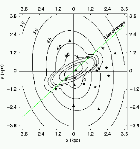
Figure 1: Projection on the sky plane ($x-y$ plane) of the column density of the LMC disk and bar. The numerical values on the contours are in $10^{7}\mathrm{M}_{\sun}\mathrm{kpc}^{-2}$ units. The three innermost contours correspond to $10$, $20$ and $30\times 10^{7}\mathrm{M}_{\sun}\mathrm{kpc}^{-2}$. The locations of the MACHO (black stars and empty diamonds) and EROS (triangles) microlensing candidates are also shown.

The column density, projected on the $x-y$ plane is plotted in Fig. 1, giving a global view of the LMC shape (disk and bar coplanar) for a terrestrial observer. We indicate the direction of the line of nodes, together with the positions of the microlensing events detected by the MACHO (filled stars and empty diamonds) and EROS (filled triangles) collaborations. The maximum value of the column density, $41.5\times 10^{7}\mathrm{M}_{\sun}\,\mathrm{kpc}^{-2}$, is assumed in the center of the LMC. The positions of the MACHO microlensing events in this $x-y$ reference system are reported in Table 1.

In order to explore the consequences of different bar geometries, besides from the coplanar configuration as in Gyuk et al. (2000) and Weinberg & Nikolaev (2001), we have considered two other possible geometries. In particular, we drop the hypothesis that the disk and bar components are dynamically connected. In a first case, drawing inspiration from the paper of Zhao & Evans (2000), we rotate the bar around an axis through the center, orthogonal to the plane defined by the bar axis and the line of sight. As a second case we shift the bar towards the observer along the line of sight as in Nikolaev et al. (2004). In both cases we change accordingly the scale parameters of the bar so as to keep its observed projected shape on the sky plane fixed. For both configurations we considered several values for the shift and the rotation angle in order to study their influence on the microlensing quantities. In the following, as an illustration, we will give the results for two somewhat extreme cases, so that we will get upper limits for the corresponding microlensing quantities

• a translation towards the observer of $\sim 0.5$ kpc;

• a rotation of $40^{\circ}$ with the south-east side towards the observer. In this case the linearly growing distance between bar and disk is $\sim 1.0$ kpc at one scale length from the center.

For the velocity dispersion of the stellar population of the bar, for which very few data are available, we take into account the qualitative results from numerical simulation that show a general trend of a higher line of sight velocity dispersion in the central region of the LMC (Zasov & Khoperskov 2002). We consider again two somewhat extreme cases: a line of sight velocity dispersion equal to that of the disk, $\sigma_{\mathrm{b,los}}=20.2$ km/s, and a second case with a higher value, $\sigma_{\mathrm{b,los}}=30$ km/s.

3.3 LMC Halo

We use two different models to describe the halo profile density: a spherical halo (model S) and an ellipsoidal halo (model E). The values of the parameters have been chosen so that the models have roughly the same mass within the same radius.

• Model S. In this model we neglect the tidal effects due to our Galaxy, and we adopt a classical pseudo-isothermal spherical density profile, which allows us to compare the results obtained in this paper with the previous ones:

  $$\rho_{\mathrm{h,S}}=\rho_{\mathrm{0,S}}\left[1+\frac{R^{2}}{a^{2}}\right]^{-1}\theta(R_{\mathrm{t}}-R),$$ (3)

  where $a$ is the LMC halo core radius, $\rho_{0,\mathrm{S}}$ the central density, $R_{\mathrm{t}}$ a cutoff radius and $\theta$ the Heaviside step function. We use $a=2$ kpc (Alcock et al. 2000a). We fix the value for the mass of the halo within a radius of 8.9 kpc equal to $5.5\times 10^{9}\mathrm{M}_{\sun}$ (van der Marel et al. 2002) that implies $\rho_{0,\mathrm{S}}$ equal to $1.76\times 10^{7}\,\mathrm{M}_{\sun}\,\mathrm{kpc}^{-3}$. Assuming a halo truncation radius, $R_{\mathrm{t}}=15$ kpc (van der Marel et al. 2002), the total mass of the halo is $\approx 1.08\times 10^{10}\,\mathrm{M}_{\sun}$.

• Model E. In this model the MW tidal effects induce a oblate spheroidal shape to the halo. We describe the halo density profile as

  $$\rho_{\mathrm{h,E}}=\rho_{\mathrm{0,E}}\left(1+\frac{1}{a^{2}}\left(\frac{\xi^{2}}{q_{1}^{2}}+\eta^{2}+\zeta^{2}\right)\right)^{-1},$$ (4)

  with $a=2$ kpc, and the truncation radius $R_{\mathrm{t}}=15$ kpc. For a LMC dark mass equal to $5.5\times 10^{9}\,\mathrm{M}_{\sun}$ within a radius of 8.9 kpc, the central density is $2.20\times 10^{7}\,\mathrm{M}_{\sun}\,\mathrm{kpc}^{-3}$, so that the LMC dark mass within the truncation radius turns out to be $\approx 1.06\times 10^{10}\,\mathrm{M}_{\sun}$.

3.4 Galactic halo

We will consider for the galactic halo a spherical model with density profile given by:

$$\rho_{\mathrm{GH}}=\rho_{\mathrm{0}}\frac{R_{\mathrm{C}}^{2}+R_{\mathrm{S}}^{2}}{R_{\mathrm{C}}^{2}+R^{2}},$$ (5)

where $R$ is the distance from the galactic center, $R_{\mathrm{C}}=5.6\,\,\mathrm{kpc}$ (Primack et al. 1988) is the core radius, $R_{\mathrm{S}}=8.5\,\,\mathrm{kpc}$ is the distance of the sun from the galactic center and $\rho_{\mathrm{0}}=7.9\times 10^{6}\,\mathrm{M}_{\sun}\,\mathrm{kpc}^{-3}$ is the mass density in the solar neighbourhood.

4 Calculation of microlensing parameters

As outlined in the introduction, here and in the following sections we want to fully exploit all the consequences of the geometry of the LMC, with the aim to shed new light on the still puzzling nature and location of the lenses detected in the microlensing surveys. In particular we study here two microlensing quantities, the optical depth and the microlensing rate.

In our analysis, whenever we need to compare models and predictions with observational results, we are going to use those presented by the MACHO collaboration only. The main reason is that this team has provided a complete description of their microlensing detection efficiency.

From the total set of 17 MACHO microlensing events one must exclude the event LMC–22, that is very likely a supernova of long duration or an active galactic nucleus in a galaxy at red-shift $z=0.23$ (Alcock et al. 2001c).

We have detailed information on LMC–5: it is due to a lens located in the Galactic disk. Indeed the lens proper motion has been observed with the HST (Alcock et al. 2001a) and the lens mass determined to be either $\simeq 0.04$ M_☉ or in the range 0.095 - 0.13 M_☉, so that it is a true brown dwarf or a M4-5V spectral type low mass star. The other stars which have been microlensed were also observed by the HST, but no other lenses have been detected. This result is also confirmed by the analysis made by von Hippel et al. (2003), by using optical and near infrared photometry on a subset of five lensing sources which are LMC main sequence stars or slightly evolved subgiants, (LMC–4, LMC–6, LMC–8, LMC–9, LMC–14). Their analysis rules out for main sequence lens masses $\geq 0.1$ M_☉ for distances out to 4 kpc.

The events LMC–9 and LMC–14 are known to be due to lenses belonging to the LMC itself, i.e. to the bar, disk or halo component. The latter event has been recognized thanks to the double source (Alcock et al. 2001b), while the first shows the characteristic caustic crossing signature of a double lens (Alcock et al. 2000b). For this reason we exclude the event LMC–9 from the following analysis, because we are interested in the study of an homogeneous set of single lens events.

We remark that LMC–5, LMC–9 and LMC–14 are the only events for which it has been possible to make a determination of the location of the lens. In Fig. 1 the events LMC–5 and LMC–9 are indicated with a special symbol, an empty diamond, whereas LMC–22 is not reported in the plot.

We use the interpolating function ${\cal E}({\hat{t}})$ of the microlensing detection efficiency, calculated by the MACHO collaboration, as a function of event timescale ${\hat{t}}$ in the interval $1-1000$ days (Fig. 5 of Alcock et al. (2000a)). It is shown in Fig. 2 by the continuous line, together with some points of the MACHO efficiency, for comparison. Let us recall that the MACHO definition of the duration time $\hat{t}$ is twice the Einstein time $T_{\mathrm{E}}$, the parameter we use in this paper. We get the following expression for ${\cal E}({\hat{t}})$:

$${\cal E}({\hat{t}})= f_{1}({\hat{t}})\,\theta[2.3-{\mathrm{Log}}\,{\hat{t}}]\,\theta[{\mathrm{Log}}\,{\hat{t}}]+$$ (6)

$$f_{2}({\hat{t}})\,\theta[{\mathrm{Log}}\,{\hat{t}}-2.3]\,\theta[2.85-{\mathrm{Log}}\,{\hat{t}}]+$$

$$f_{3}({\hat{t}})\,\theta[{\mathrm{Log}}\,{\hat{t}}-2.85]\,\theta[3-{\mathrm{Log}}\,{\hat{t}}]\;,$$

with $\theta$ the Heaviside function, and

$$f_{1}({\hat{t}})= {\frac{{\mathrm{Log}}^{3}\,{\hat{t}}}{{\hat{t}}^{1.97}}}\left[8\,{\mathrm{Log}}^{5}\,{\hat{t}}+{\frac{49}{40}}{\mathrm{Log}}^{8}\,{\hat{t}}\right]$$ (7)

$$f_{2}({\hat{t}})= {\frac{f_{1}(10^{2.3})-{\frac{125}{64}}\left({\mathrm{Log}}\,{\hat{t}}-2.3\right)^{3}}{10^{\left(2.3-{\mathrm{Log}}\,{\hat{t}}\right)^{4}}}}$$ (8)

$$f_{3}({\hat{t}})= 0.06+\left[f_{2}(10^{2.85})-0.06\right]e^{10(2.85-{\mathrm{Log}}\,{\hat{t}})}\;.$$ (9)

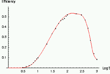
Figure 2: Plot of the interpolating function ${\cal E}({\hat{t}})$ of the MACHO detection efficiency.

As described in the previous section, the LMC has its own halo, with a tidal radius $R_{\mathrm{t}}=15.0\pm 4.5$ kpc. Assuming that the galactic halo extends to at least 65 kpc, a fraction of the LMC halo total mass, enclosed in a sphere of radius $R_{\mathrm{t}}$, is attributable to the galactic halo. A simple calculation gives the galactic halo mass enclosed in a sphere centered on the LMC with a radius of 8.9 kpc to be $9.7\times 10^{8}\,\mathrm{M}_{\sun}$, a value corresponding to a sensible fraction of the LMC halo mass, of the order of $\simeq 17\%$. We will take into account this fact, by properly correcting the value of the central density of the LMC halo: for the spherical model the value is decreased to $\rho_{0,\mathrm{S}}=1.45\times 10^{7}\,\mathrm{M}_{\sun}\,\mathrm{kpc}^{-3}$ and the corresponding total LMC halo mass inside the tidal radius $R_{\mathrm{t}}$ is $\approx 8.86\times 10^{9}\,\mathrm{M}_{\sun}$; for the ellipsoidal model the value is decreased to $\rho_{0,\mathrm{E}}=1.81\times 10^{7}\,\mathrm{M}_{\sun}\,\mathrm{kpc}^{-3}$ and the corresponding total LMC halo mass inside the tidal radius $R_{\mathrm{t}}$ is $\approx 8.7\times 10^{9}\,\mathrm{M}_{\sun}$.

4.1 Optical depth

We now discuss the results obtained for the optical depth. The computation is made by weighting the optical depth with respect to the distribution of the source stars along the line of view. We use Eq. (7), Sect. 3.1, of Paper I, that we report here for self consistency reasons:

$$\tau={\frac{4\pi G}{c^{2}}}{\frac{\int_{0}^{\infty}\left[\int_{0}^{D_{\mathrm{os}}}{\frac{D_{\mathrm{ol}}(D_{\mathrm{os}}-D_{\mathrm{ol}})}{D_{\mathrm{os}}}}\rho_{\mathrm{l}}\,dD_{\mathrm{ol}}\right]\rho_{\mathrm{s}}\,dD_{\mathrm{os}}}{\int_{0}^{\infty}\rho_{\mathrm{s}}\,dD_{\mathrm{os}}}}\;,$$ (10)

where $\rho_{\mathrm{l}}$ denotes the mass density of the lenses, $\rho_{\mathrm{s}}$ the mass density of the sources, $D_{\mathrm{ol}}$ and $D_{\mathrm{os}}$, respectively, the distance observer-lens and observer-source.

The contour maps reported in Figs. 3, 4, 5 and 6 refer to the case of coplanarity between bar and disk. In Fig. 3 is reported the optical depth contour map for lenses in the Galactic halo, in the hypothesis that all the Galactic dark halo consists of compact lenses, together with the positions of the MACHO fields (see Fig. 14 for the numeration of the fields), the microlensing events and the van der Marel line of nodes. We observe that almost all the fields (except three of them) fall between the contour lines corresponding to $\tau=46.3\times 10^{-8}$ and $\tau=49.3\times 10^{-8}$. As expected the optical depth due to the galactic halo is a slowly variable function, and presents a slight near-far asymmetry: moving from the nearer to the farther fields along a line passing through the center and perpendicular to the line of nodes, the increase of the optical depth is of the order of $\approx 6\%$.

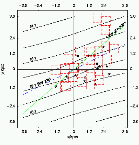
Figure 3: Contour map of the optical depth for lenses in the galactic halo. The locations of the MACHO fields and of the microlensing candidates are also shown. The numerical values are in $10^{-8}$ units.

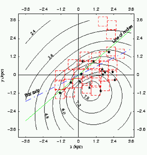
Figure 4: Model S: contour map of the optical depth for lenses in the LMC halo. The locations of the MACHO fields and of the microlensing candidates are also shown. The numerical values are in $10^{-8}$ units.

In Figs. 4 and 5 we report the optical depth contour maps for lenses belonging to the halo of the LMC, assuming a spherical and an ellipsoidal shape, respectively, in the hypothesis that all the LMC dark halo consists of compact lenses. A striking feature of both maps is the strong near-far asymmetry.

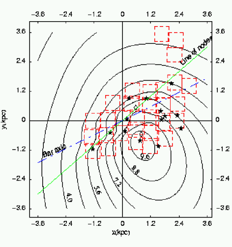
Figure 5: Model E: contour map of the optical depth for lenses in the LMC halo. The locations of the MACHO fields and of the microlensing candidates are also shown. The numerical values are in $10^{-8}$ units.

For the Model S, the maximum value of the optical depth, $\tau_{\mathrm{max,S}}\simeq 8.05\times 10^{-8}$, is assumed in a point falling in the field number 13, belonging to the fourth quadrant, at a distance of $\simeq 1.27$ kpc from the center. The value in the point symmetrical with respect to the center, belonging to the second quadrant and falling about at the upward left corner of the field 82, is $\tau_{\mathrm{S}}\simeq 4.30\times 10^{-8}$. The increment of the optical depth is of the order of $\approx 87\%$, moving from the nearer to the farther fields.

The same happens for the model E: the maximum value of the optical depth, $\tau_{\mathrm{max,E}}\simeq 9.88\times 10^{-8}$, higher than the previous one, is found at about the same point, at the same distance from the center. In the symmetrical point with respect to the center, belonging to the field 82, the optical depth is $\tau_{\mathrm{E}}\simeq 5.05\times 10^{-8}$. The ellipsoidal shape of the LMC halo gives rise to a further enhancement of the near-far asymmetry, with an increase of the optical depth by $\approx 95\%$.

One can draw advantage from the different asymmetric behaviour of the optical depth in the two cases of lenses in the galactic halo or in the LMC halo, both to confirm the existence of a proper LMC halo and to disentangle the microlensing events due to the Galactic halo from the ones due to the LMC halo. To this end, a good observation strategy would help, the goal being to allow the analysis of asymmetry of microlensing events belonging to two equivalent regions, placed symmetrically with respect to the line of nodes. An example of the kind of analysis and of results one could obtain is given in Sect. 5.

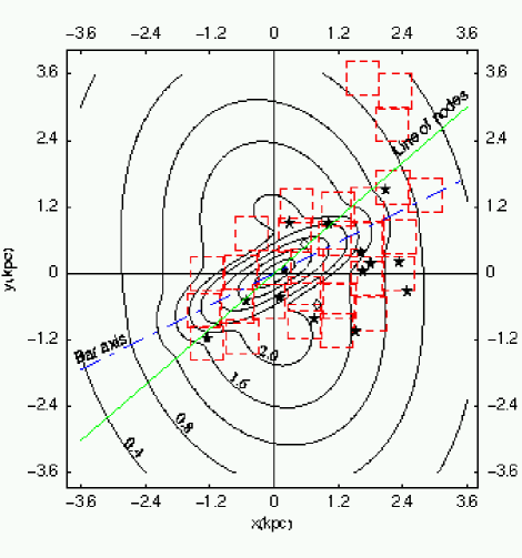
Figure 6: Contour map of the optical depth for self lensing. The locations of the MACHO fields and of the microlensing candidates are also shown. The numerical values are in $10^{-8}$ units. The innermost contours correspond to values $2.4\times 10^{-8}$, $3.2\times 10^{-8}$, $4.0\times 10^{-8}$ and $4.6\times 10^{-8}$ respectively.

In Fig. 6 we report the optical depth contour map for self lensing, i. e. for events where both the sources and the lenses belong to the stellar population of the disk and/or the bar of the LMC. As expected, there is almost no near-far asymmetry and the maximum value of the optical depth, $\tau_{\mathrm{max}}\simeq 4.90\times 10^{-8}$, is reached in the center of the LMC. The optical depth then rapidly decreases, when moving, for instance, along a line going through the center and perpendicular to the minor axis of the elliptical disk, that coincides also with the major axis of the bar. In a range of about only $0.80\,\mathrm{kpc}$ the optical depth quickly falls to $\tau\simeq 2\times 10^{-8}$, and afterwards it decreases slowly to lower values.

The calculated value of the optical depth in the center seems at first glance to be in contradiction with the value one gets using the Gould inequality (Gould 1995):

$$\tau\leq 2{\frac{<v^{2}>}{c^{2}}}\sec^{2}i\approx 1.34\times 10^{-8}.$$ (11)

In fact, this inequality is derived making some simplifying assumptions which do not fully apply to our choice of the density profiles for the disk and the bar. In Sect. 6 we shall derive an improved version of the Gould inequality, which will also apply to our density profile and leads to $\tau\leq 6\times 10^{-8}$, which does not contradict our above estimated value.

Furthermore, we recall that the Gould inequality is obtained under the hypothesis that the LMC is a virialized system, that quite likely is note the case for some of its components. This should of course be taken into account when using it in comparison with the observations.

As expected, the changes of the geometry as discussed in Sect. 3.2, where we allow for a non coplanar morphology of the bar with respect to the disk, enhance the self–lensing optical depth in the bar region considerably (up to $\sim$ 50%). On the other hand, the changes for the optical depth for lenses in the MW halo are negligible (at maximum $\sim$ 1%). For lenses in the LMC halo the variations, in the innermost region of the LMC, can be rather large (up to $\sim$ 20%). However, the main feature that interests us, the near–far asymmetry due to the disk inclination, is not altered. Besides, as we are here mainly concerned with the self–lensing case, we do not discuss them any further. In any case, outside the bar region, these differences drop abruptly to zero.

For a rotated bar, Fig. 7, the increment of the self–lensing optical depth, with respect to the symmetric coplanar case, is slightly asymmetric with respect to the bar major axis. This is due to the different variations of the source–lens distances between the west side, where the sources are in the bar and the lenses in the disk, and the east side, where the opposite happens. The relative increment can be as large as $\approx 50\,\%$.

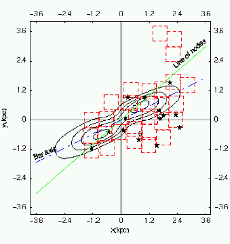
Figure 7: Contour map of the difference between the self–lensing optical depth calculated in the case of $+40^{\circ}$ rotated bar and the one with coplanar bar and disk. Going from the outer to the inner part, the contours correspond to increasing values of the difference: $0.1,\,0.6,\,1.1\,{\mathrm{and}}\,1.6\times 10^{-8}$. The difference is null outside the bar region.

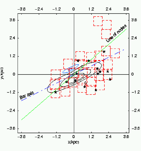
Figure 8: Contour map of the difference between the self–lensing optical depth calculated in the case of $0.5$ kpc shifted bar and the one with coplanar bar and disk. Going from the outer to the inner part, the black contours correspond to increasing positive values of the difference: $+0.1,\,+0.5,\,+0.9,\,{\mathrm{and}}\,+1.3\times 10^{-8}$; the lighter contours to negative values of the difference: $-0.1,\,{\mathrm{and}}\,-0.2\times 10^{-8}$.

When we allow for a translation of the bar, Fig. 8, the variation of the optical depth, with respect to the coplanar case, is higher in the region below the bar major axis (south-west side), even if the projected density of the bar is the same as shown in Fig. 1. This is induced by the inclination of the disk plane, that gives rise to increasing distances between the bar and the disk plane for lines of sight towards the lower part of the bar. In this case we find also a small region with a negative difference of the optical depth, shown by the lighter contour lines (north-east side). The relative increment can be as large as $\approx 35\,\%$.

It is interesting to note that a larger statistics of observed events in the central region might eventually allow one to discriminate between the different bar models.

We notice also that, due to the loss of the symmetry, the Gould inequality no longer applies in these cases.

4.2 Self lensing microlensing event rate

The distribution $\frac{\mathrm{d}\Gamma}{\mathrm{d}\,T_{\mathrm{E}}}$, the differential rate of microlensing events with respect to the Einstein time $T_{\mathrm{E}}$, allows one to estimate the expected typical duration and the expected number of the microlensing events. In this paper we evaluate the microlensing rate in the self–lensing configuration, i. e. lenses and sources both in the disk and/or in the bar of the LMC. We take into account also the transverse motion of the Sun and of the source stars.

We assume that, to an observer comoving with the LMC center, the velocity distribution of the source stars and lenses have a Maxwellian profile. Moreover, since the component parallel to the line of view is irrelevant to microlensing, we integrate over the parallel component. Therefore, the two–dimensional transverse velocity distribution of the source and lens stars is:

$$f({\tilde{\@vec{v}}}_{\perp})\,\mathrm{d}^{2}{\tilde{v}}_{\perp}={\frac{1}{2\,\pi\sigma_{\mathrm{los}}^{2}}}\,e^{\left({-{\frac{{\tilde{{v}}}_{\perp}^{2}}{2\,\sigma_{\mathrm{los}}^{2}}}}\right)}\,{\tilde{v}}_{\perp}\,\mathrm{d}{\tilde{v}}_{\perp}\,\mathrm{d}\varphi\;,$$ (12)

where we have used cylindrical coordinates d${}^{2}{\tilde{v}}_{\perp}={\tilde{v}}_{\perp}\,\mathrm{d}{\tilde{v}}_{\perp}\,\mathrm{d}\phi$.

With respect to an observer comoving with the LMC center, the transverse velocity of the microlensing tube at position $D_{\mathrm{ol}}=x\,D_{\mathrm{os}}$ ($0\leq x\leq 1$) is given by ${\tilde{\@vec{v}}}_{\mathrm{t}\perp}=(1-x)\,{{\tilde{\@vec{v}}}_{\sun\perp}}+x\,{\tilde{\@vec{v}}}_{\mathrm{s}\perp}$, where $\tilde{\@vec{v}}_{\mathrm{s}\perp}$ is the velocity of the source, and $\tilde{\@vec{v}}_{\sun\perp}$ represents the Sun velocity in the plane orthogonal to the line of sight, as measured by an observer comoving with the LMC center. It results $|{\tilde{\@vec{v}}}_{\sun\perp}|\simeq 406$ km/s (van der Marel et al. 2002).

Let us consider a segment of cylindrical ring at position $x$, of length d$D_{\mathrm{ol}}$, with radius equal to the Einstein radius

$$R_{\mathrm{E}}=\left({\frac{4\,G\,\mathrm{M}_{\sun}}{c^{2}}}\,{\mu\,D_{\mathrm{os}}\,x(1-x)}\right)^{\frac{1}{2}}\;,$$

angular amplitude d$\alpha$ and thickness $({\hat{\@vec{v}}}_{\mathrm{l}\perp}\cdot\hat{n})\,\mathrm{d}t={\hat{v}}_{\mathrm{l}\perp}\,\cos\theta\,\mathrm{d}t$, where $-\,{\frac{\pi}{2}}\leq\theta\leq{\frac{\pi}{2}}$ is the angle between the inner normal to the cylindrical ring segment and the vector ${\hat{\@vec{v}}}_{\mathrm{l}\perp}$. ${\hat{\@vec{v}}}_{\mathrm{l}\perp}$ represents the lens velocity in the plane orthogonal to the line of sight, as measured by an observer comoving with the microlensing tube at position $x$. We use solar mass units, defining $\mu={\frac{M}{\mathrm{M}_{\sun}}}$, where $M$ is the lens mass. The number of lenses with mass in the range $(\mu,\,\mu+\mathrm{d}\mu)$ inside the volume element of the cylindrical ring segment is equal to the product of the differential number density of the lenses ${\frac{\mathrm{d}\,n_{\mathrm{l}}}{\mathrm{d}\,\mu}}\,\mathrm{d}\,\mu$ by the volume element ${\hat{v}}_{\mathrm{l}\perp}\cos\theta\,R_{\mathrm{E}}\,\mathrm{d}t\,\mathrm{d}\alpha\,\mathrm{d}D_{\mathrm{ol}}$. The fraction entering in the time interval d$t$ in the microlensing tube with transverse velocity ${\hat{\@vec{v}}}_{\mathrm{l}\perp}$, is given by those lenses that with respect to the LMC reference frame have velocity

$${\tilde{\@vec{v}}}_{\mathrm{l}\perp}={\hat{\@vec{v}}}_{\mathrm{l}\perp}+\tilde{\@vec{v}}_{\mathrm{t}\perp}={\hat{\@vec{v}}}_{\mathrm{l}\perp}+(1-x)\,{\tilde{\@vec{v}}_{\sun\perp}}+x\,\tilde{\@vec{v}}_{\mathrm{s}\perp}\;.$$ (13)

In the self–lensing case, $x\simeq 1$, and to first approximation we can neglect the term proportional to $(1-x)$. As a consequence the velocity distribution with respect to the microlensing tube, in the general case of two different values for the velocity dispersion, is given by:

$${\frac{{\hat{v}}_{\mathrm{l}\perp}\,\mathrm{d}{\hat{v}}_{\mathrm{l}\perp}\,\mathrm{d}\theta}{2\,\pi\,\left[\rho_{\mathrm{d}}(x)+\rho_{\mathrm{b}}(x)\right]}}\left[e^{\left(-{\frac{{\hat{v}}_{\mathrm{l}\perp}^{2}+2\,x\,{\hat{v}}_{\mathrm{l}\perp}\,{\tilde{v}}_{\mathrm{s}\perp}\,\cos(\alpha-\theta)+x^{2}\,{\tilde{v}}_{\mathrm{s}\perp}^{2}}{2\,\sigma_{\mathrm{d}}^{2}}}\right)}\right.\cdot$$

$$\left.{\frac{\rho_{\mathrm{d}}(x)}{\sigma_{\mathrm{d}}^{2}}}+e^{\left(-{\frac{{\hat{v}}_{\mathrm{l}\perp}^{2}+2\,x\,{\hat{v}}_{\mathrm{l}\perp}\,{\tilde{v}}_{\mathrm{s}\perp}\,\cos(\alpha-\theta)+x^{2}\,{\tilde{v}}_{\mathrm{s}\perp}^{2}}{2\,\sigma_{\mathrm{b}}^{2}}}\right)}{\frac{\rho_{\mathrm{b}}(x)}{\sigma_{\mathrm{b}}^{2}}}\right] =$$

$${\frac{{\hat{v}}_{\mathrm{l}\perp}\,\mathrm{d}{\hat{v}}_{\mathrm{l}\perp}\,\mathrm{d}\theta}{2\,\pi\,\left[\rho_{\mathrm{d}}(x)+\rho_{\mathrm{b}}(x)\right]}}\,h(\rho_{\mathrm{d}},\sigma_{\mathrm{d}};\,\rho_{\mathrm{b}},\sigma_{\mathrm{b}};\,x,{\hat{v}}_{\mathrm{l}\perp},{\tilde{v}}_{\mathrm{s}\perp};\,\alpha,\theta)\,$$ (14)

where $\sigma_{\mathrm{d}}\equiv\sigma_{\mathrm{d,los}}$, $\sigma_{\mathrm{b}}\equiv\sigma_{\mathrm{b,los}}$ and $\alpha$ is the angle that the segment of cylindrical ring at position $x$, of angular amplitude d$\alpha$, forms with the direction of the orthogonal component to the line of sight of the velocity vector of the source star, $\tilde{\@vec{v}}_{\mathrm{s}\perp}$.

We need now to specify the form of the number density. Assuming that the mass distribution of the lenses is independent of their position in the LMC (factorization hypothesis (de Rújula et al. 1995)), the lens number density per unit mass is given by

$${\frac{\mathrm{d}n_{\mathrm{l}}}{\mathrm{d}\mu}}={\frac{\rho_{\mathrm{d}}+\rho_{\mathrm{b}}}{\mathrm{M}_{\sun}}}\,{\frac{\mathrm{d}n_{0}}{\mathrm{d}\mu}},$$ (15)

where we use ${\frac{\mathrm{d}n_{0}}{\mathrm{d}\mu}}$ as given in Chabrier (2001). We consider both the power law and the exponential initial mass functions. However, we find that our results do not depend strongly on that choice and hereafter, we will discuss the results we obtain by using the exponential IMF only.

Let us note that, considering the experimental conditions for the observations of the MACHO team, we use as range of variability for the lens masses $0.08\leq\mu\leq 1.5$. Namely the lower limit is fixed by the requirement that the lenses belong to the luminous component of the LMC, while the upper limit is fixed by the requirement that the lenses are not resolved stars.

The total differential rate d$\Gamma$ at which lenses enter the portion of the microlensing tube at position $x$, along a fixed line of sight, is given by (de Rújula et al. 1991; Griest 1991):

$$\mathrm{d}\,\Gamma = {\frac{{\hat{v}}_{\mathrm{l}\perp}^{2}\,d{\hat{v}}_{\mathrm{l}\perp}}{4\,\pi^{2}{\cal N}\,\mathrm{M}_{\sun}}}\,\int_{0}^{2\,\pi}\mathrm{d}\varphi\int_{-{\frac{\pi}{2}}}^{{\frac{\pi}{2}}}\,\mathrm{d}\theta\,\,{{\cos\theta}}\,\cdot$$ (16)

$$\int_{d_{\mathrm{min}}}^{d_{\mathrm{max}}}D_{\mathrm{os}}\,dD_{\mathrm{os}}\int_{\frac{d_{\mathrm{min}}}{D_{\mathrm{os}}}}^{1}\mathrm{d}x\,\int_{0.08}^{1.5}\mathrm{d}\mu\,{\frac{\mathrm{d}n_{0}}{\mathrm{d}\mu}}\,R_{\mathrm{E}}\,\cdot$$

$$\int_{0}^{\infty}\mathrm{d}{\tilde{v}}_{\mathrm{s}\perp}{{\tilde{v}}_{\mathrm{s}\perp}}\left[{\frac{\rho_{\mathrm{d}}(D_{\mathrm{os}})}{\sigma_{\mathrm{d}}^{2}}}\,e^{-{\frac{{\tilde{v}}_{\mathrm{s}\perp}^{2}}{2\,\sigma_{\mathrm{d}}^{2}}}}+{\frac{\rho_{\mathrm{b}}(D_{\mathrm{os}})}{\sigma_{\mathrm{b}}^{2}}}\,e^{-{\frac{{\tilde{v}}_{\mathrm{s}\perp}^{2}}{2\,\sigma_{\mathrm{b}}^{2}}}}\right]\cdot$$

$$\int_{0}^{2\,\pi}\mathrm{d}\alpha\,h(\rho_{\mathrm{d}},\sigma_{\mathrm{d}};\,\rho_{\mathrm{b}},\sigma_{\mathrm{b}};\,x,{\hat{v}}_{\mathrm{l}\perp},{\tilde{v}}_{\mathrm{s}\perp};\,\alpha,\theta)$$

where

$${\cal N}=\int_{d_{\mathrm{min}}}^{d_{\mathrm{max}}}\mathrm{d}D_{os}\,\left[\rho_{\mathrm{d}}(D_{\mathrm{os}})+\rho_{\mathrm{b}}(D_{\mathrm{os}})\right],$$

having assumed that the number of detectable stars varies with the distance as $D_{\mathrm{os}}^{-2}$. The integration limits $d_{\mathrm{min}}$, $d_{\mathrm{max}}$ represent the distances from the observer of the intersection points of the line of sight with the LMC tidal surface.

Finally, as we are interested in the distribution $\frac{\mathrm{d}\Gamma}{\mathrm{d}T_{\mathrm{E}}}$, we change variable from ${\hat{v}}_{\mathrm{l}\perp}$ to $T_{\mathrm{E}}$, bearing in mind that ${\hat{v}}_{\mathrm{l}\perp}={\frac{R_{\mathrm{E}}}{T_{\mathrm{E}}}}$. After integration on $\varphi$, $\theta$ and $\alpha$, and taking into account the detection efficiency function, Eq. (6), we obtain:

$$\left({\frac{\mathrm{d}\Gamma}{\mathrm{d}T_{\mathrm{E}}}}\right)_{\varepsilon} = {\frac{\mathrm{d}\Gamma}{\mathrm{d}T_{\mathrm{E}}}}\,\cdot\,{\cal E}(T_{\mathrm{E}})={\frac{32\,G^{2}\,\mathrm{M}_{\sun}\,{\cal E}(T_{\mathrm{E}})}{c^{4}\,T_{\mathrm{E}}^{4}\,{\cal N}}}\,\,\cdot$$ (17)

$$\int_{d_{\mathrm{min}}}^{d_{\mathrm{max}}}\mathrm{d}D_{\mathrm{os}}\,D_{\mathrm{os}}^{3}\,\cdot$$

$$\int_{\frac{d_{\mathrm{min}}}{D_{\mathrm{os}}}}^{1}\mathrm{d}x\,x^{2}\,(1-x)^{2}\int_{0.08}^{1.5}\mathrm{d}\mu\,\mu^{2}\,{\frac{\mathrm{d}n_{0}}{\mathrm{d}\mu}}\cdot$$

$$\left[{\frac{\rho_{\mathrm{b}}(x)\rho_{\mathrm{b}}(D_{\mathrm{os}})}{(1+x)^{2}\sigma_{\mathrm{b}}^{2}}}\,e^{\left(-{\frac{2\,G\,\mathrm{M}_{\sun}\,D_{\mathrm{os}}\,x\,(1-x)\,\mu}{c^{2}\,(1+x^{2})\,\sigma_{\mathrm{b}}^{2}\,T_{\mathrm{E}}^{2}}}\right)}\right.+$$

$${\frac{\rho_{\mathrm{d}}(x)\rho_{\mathrm{b}}(D_{\mathrm{os}})}{\sigma_{\mathrm{d}}^{2}+x^{2}\sigma_{\mathrm{b}}^{2}}}\,e^{\left(-{\frac{2\,G\,\mathrm{M}_{\sun}\,D_{\mathrm{os}}\,x\,(1-x)\,\mu}{c^{2}\,(\sigma_{\mathrm{d}}^{2}+x^{2}\sigma_{\mathrm{b}}^{2})\,T_{\mathrm{E}}^{2}}}\right)}+$$

$${\frac{\rho_{\mathrm{b}}(x)\rho_{\mathrm{d}}(D_{\mathrm{os}})}{\sigma_{\mathrm{b}}^{2}+x^{2}\sigma_{\mathrm{d}}^{2}}}\,e^{\left(-{\frac{2\,G\,\mathrm{M}_{\sun}\,D_{\mathrm{os}}\,x\,(1-x)\,\mu}{c^{2}\,(\sigma_{\mathrm{b}}^{2}+x^{2}\sigma_{\mathrm{d}}^{2})\,T_{\mathrm{E}}^{2}}}\right)}+$$

$$\left.{\frac{\rho_{\mathrm{d}}(x)\rho_{\mathrm{d}}(D_{\mathrm{os}})}{(1+x)^{2}\sigma_{\mathrm{d}}^{2}}}\,e^{\left(-{\frac{2\,G\,\mathrm{M}_{\sun}\,D_{\mathrm{os}}\,x\,(1-x)\,\mu}{c^{2}\,(1+x^{2})\,\sigma_{\mathrm{d}}^{2}\,T_{\mathrm{E}}^{2}}}\right)}\right]$$

In the following section we need also the two distributions

$$\left({\frac{\mathrm{d}^{2}\Gamma}{\mathrm{d}T_{\mathrm{E}}\,\mathrm{d}x}}\right)_{\varepsilon}=\left.{\cal E}(T_{\mathrm{E}})\,{\frac{\mathrm{d}^{2}\Gamma}{\mathrm{d}T_{\mathrm{E}}\,\mathrm{d}x}}\right|_{T_{\mathrm{E,event}}}$$ (18)

$$\left({\frac{\mathrm{d}^{2}\Gamma}{\mathrm{d}T_{\mathrm{E}}\,\mathrm{d}\mu}}\right)_{\varepsilon}=\left.{\cal E}(T_{\mathrm{E}})\,{\frac{\mathrm{d}^{2}\,\Gamma}{\mathrm{d}\,T_{\mathrm{E}}\,\mathrm{d}\mu}}\right|_{T_{\mathrm{E,event}}}$$ (19)

calculated assigning to $T_{\mathrm{E}}$ the corresponding effective measured value.

4.3 A statistical analysis for self–lensing events discrimination

In this section we will show that, in the framework of the LMC geometrical structure and dynamics outlined in Sect. 3, a suitable statistical analysis allows us to exclude from the self–lensing population a large subset of the detected events. To this purpose, assuming all the 15 events as self lensing, we study the scatter plots correlating the self lensing expected values of some meaningful microlensing variables with the measured Einstein time or with the self–lensing optical depth. The idea underlying this analysis is based on the search of self–lensing average collective properties with different behaviour in the two different regions of the LMC: the bar with its nearby neighbourhood and the disk region external to it. In this way we eventually show that a large subset of events is incompatible with the self–lensing hypothesis.

We have calculated the self–lensing distributions $\left({\frac{\mathrm{d}\Gamma}{\mathrm{d}T_{\mathrm{E}}}}\right)_{\varepsilon}$ of the rate of microlensing events with respect to the Einstein time $T_{\mathrm{E}}$, along the lines of sight towards the 15 events of the MACHO collaboration, in the case of a Chabrier exponential type IMF. As an example we show in Fig. 9 the distributions $\left({\frac{\mathrm{d}\Gamma}{\mathrm{d}T_{\mathrm{E}}}}\right)_{\varepsilon}$ calculated along the lines of sight pointing towards the events LMC–1 (solid line), LMC–8 (dashed line) and LMC–23 (dot dashed line).

With these distributions we have calculated the median $T_{\mathrm{E},\,50\,\%}$ and the values $T_{\mathrm{E},\,16\,\%}$ and $T_{\mathrm{E},\,84\,\%}$ that single out the extremes of the 68% probability range around the median (not to be confused with a 1$\sigma$ error). In Table 1 we report these values for each observed MACHO event.

event	x (kpc)	y (kpc)	$T_{\mathrm{E,obs}}$	$T_{\mathrm{E,50\%}}$	$T_{\mathrm{E,16\%}}$	$T_{\mathrm{E,84\%}}$
1	1.017	0.909	22.3	64	33	126
4	0.746	-0.814	29.5	66	35	128
5	0.797	-0.559	49.1	65	34	127
6	0.102	-0.423	59.5	55	28	111
7	1.796	0.189	66.8	73	38	140
8	0.185	0.062	43.1	48	25	95
13	0.280	0.916	65.0	66	33	128
14	-0.523	-0.487	65.0	51	26	103
15	1.652	0.048	23.9	72	38	137
18	-1.253	-1.168	48.2	72	38	138
20	2.478	-0.316	47.2	77	40	146
21	2.324	0.211	60.5	77	40	146
23	1.517	-1.037	55.4	72	38	138
25	2.072	1.517	55.4	79	41	149
27	1.619	0.388	32.8	67	34	130

Table 1: Microlensing rate: the results for the predicted Einstein time. Case with disk and bar coplanar and bar velocity dispersion $\sigma_{\mathrm{b}}=20.2$ km/s. For each observed MACHO event we report for the Einstein time (days): the observed value and the predicted median value with the two extreme of a 68% probability range around it. In the second and third column we report the position in the reference frame centered in the LMC as defined in Sect. 3.

Trying to see if the geometry can help, we have analyzed how the self–lensing expected values of $T_{\mathrm{E}}$ depend on the position, or better still on the optical depth, taking into account that the LMC disk symmetry is elliptical and not circular.

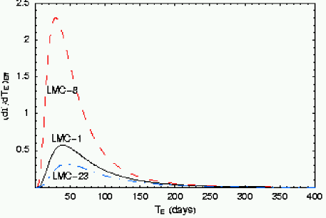
Figure 9: Differential rate of the microlensing events with respect to the Einstein time $T_{\mathrm{E}}$, along the lines of sight pointing towards the events LMC–8 (dashed red line), LMC–1 (solid black line) and LMC–23 (dot dashed blue line). The $y$–axis values are in $10^{-12}$ units.

In Fig. 10 we report on the $y$–axis the observed values of $T_{\mathrm{E}}$ (empty boxes) as well as the expected values for self lensing of the median $T_{\mathrm{E}\,,50\,\%}$ (filled circle) evaluated along the directions of the events. On the $x$–axis we report the value of the self–lensing optical depth calculated towards the event position. The optical depth increases as one moves from the outer regions towards the center of the LMC according to the contour lines shown in Fig. 6. An interesting feature emerging clearly is the decreasing trend of the expected values of the median $T_{\mathrm{E}\,,50\,\%}$, going from the outside fields with low values of $\tau_{\mathrm{SL}}$ towards the central fields with higher values of $\tau_{\mathrm{SL}}$. The variation of the stellar number density and the flaring of the LMC disk certainly contributes to explain this behaviour.

We now tentatively identify two subsets of events: the ten falling outside the contour line $\tau_{\mathrm{SL}}=2\times 10^{-8}$ of Fig. 6 and the five falling inside. In the framework of van der Marel et al. LMC geometry, this contour line includes almost fully the LMC bar and two ear shaped inner regions of the disk, where we expect self–lensing events to be located with higher probability.

At first glance, we note that the two clusters have a clear-cut different collective behaviour: the measured Einstein times of the first 10 points fluctuate around a median value of 47 days, very far from the expected values of the median $T_{\mathrm{E}}$, ranging from 65 days to 79 days, with an average value of 72 days. On the contrary, for the last 5 points, the measured Einstein times fluctuate around a median value of 51 days, near to the average value 57 days of the expected medians, ranging from 48 days to 66 days. Let us note, also, the somewhat peculiar position of the event LMC–1, with a very low value of the observed $T_{\mathrm{E}}$. In the following analysis it will be shown that most probably this event is homogeneous to the set at left of the vertical line in Fig. 10 and it has to be included in that cluster.

This plot gives a first clear evidence that, in the framework of van der Marel et al. LMC geometry, the self–lensing events have to be searched among the cluster of events with $\tau_{\mathrm{SL}}\,>\,2\times 10^{-8}$, and at the same time that the cluster of the $10$ events plus LMC–1 belongs, very probably, to a different population.

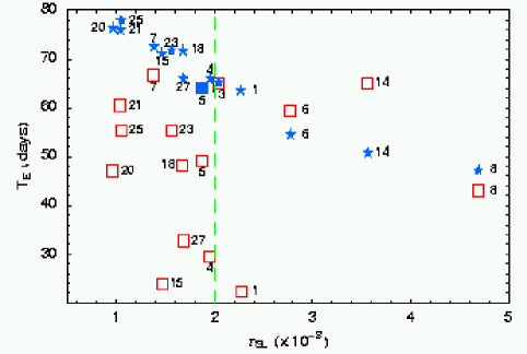
Figure 10: Scatter plot of the observed (empty boxes) values of the Einstein time and of the expected values of the median $T_{\mathrm{E},50\,\%}$ (filled stars), with respect to the self–lensing optical depth evaluated along the directions of the events. The $T_{\mathrm{E},50\,\%}$ for the galactic disk event LMC–5 is represented by a filled box.

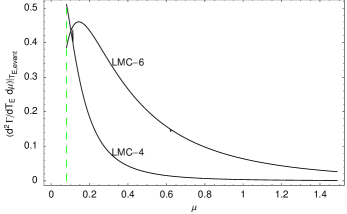
Figure 11: Differential rate of the microlensing events with respect to the mass of the lens in direction of events LMC–4 and LMC–6. The dashed vertical line is at $\mu=0.08$. The y axis values are in $10^{-3}$ units.

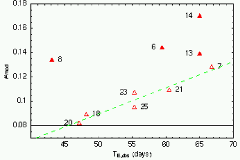
Figure 12: Scatter plot of the modal value of $\mu$ ($y$–axis) with respect to the measured Einstein time ($x$–axis) of each event. The label identifies the event. Filled (empty) triangles represent points with $\tau_{\mathrm{SL}}\,>\,2\times 10^{-8}\,(<\,2\times 10^{-8})$. The horizontal line indicates the lower limit of the lens mass for self lensing, $\mu=0.08$. The four events LMC–1, LMC–4, LMC–15 and LMC—27 have a modal value of the lens mass smaller than the lower limit and therefore are not represented. The dashed line represents the correlation line for the $6$ events with $\tau_{\mathrm{SL}}\,<\,2\times 10^{-8}$.

In order to further improve our statistical analysis, we have calculated the distributions $\left({\frac{\mathrm{d}^{2}\Gamma}{\mathrm{d}T_{\mathrm{E}}\,\mathrm{d}\mu}}\right)_{\varepsilon}$ along the lines of sight pointing towards the 14 LMC microlensing events, taking, for each line of sight, the observed Einstein time value. As an example we show in Fig. 11 this distribution calculated for the two events LMC–6 and LMC–4. LMC–6 is representative of the events for which the modal value $\mu_{\mathrm{mod}}$ falls inside the self–lensing mass interval 0.08–1.5. The second one has been chosen to put in evidence that there are also events for which $\mu_{\mathrm{mod}}$ falls outside, in the range 0–0.08.

Fig. 12 is the scatter plot between the measured $T_{\mathrm{E}}$ ($x$–axis) and the modal value of the lens mass $\mu={\frac{M_{\mathrm{l}}}{\mathrm{M}_{\sun}}}$ ($y$–axis), calculated by the distribution $\left({\frac{\mathrm{d}^{2}\Gamma}{\mathrm{d}T_{\mathrm{E}}\,\mathrm{d}\mu}}\right)_{\varepsilon}$. In this case we prefer to use the modal value rather than the median one, because it is independent of the amplitude of the interval of the allowed values of the lenses mass, whereas the median value varies in accordance with this choice.

We find that the events LMC–1, LMC–4, LMC–15 and LMC–27 have a modal value of the lens mass smaller than the lower limit. We consider this result as a strong indication to exclude these four events from the self–lensing class. We have then calculated the linear correlation between $\mu_{\mathrm{mod}}$ and $T_{\mathrm{E}}$ for the 6 remaining points out of the cluster of ten. We find a high linear correlation, as shown by the dashed green straight line in Fig. 12 and by the calculated linear correlation coefficient equal to $0.963$. We observe that the values of $\mu_{\mathrm{mod}}$ of the six events range between 0.08 and 0.13, an interval narrow enough to justify the linear approximation to represent a small portion of a parabolic curve, around which we expect the correlated points to disperse, bearing in mind that $T_{\mathrm{E}}$ is proportional to $\sqrt{\mu}$. The six linearly correlated events, therefore, constitute a homogeneous population, clearly distinct, also in this parameter space, from that formed by events with $\tau_{\mathrm{SL}}\,>\,2\times 10^{-8}$ for which, for a given value of the observed Einstein time, we get significantly higher values for the mass.

We have calculated also the distributions $\left({\frac{\mathrm{d}^{2}\Gamma}{\mathrm{d}T_{\mathrm{E}}\,\mathrm{d}x}}\right)_{\varepsilon}$ along the lines of sight pointing towards the 14 LMC microlensing events, in order to obtain a second independent check of the homogeneity of the cluster of events with $\tau_{SL}\leq 2\times 10^{-8}$. Fig. 13 is the scatter plot between the measured $T_{E}$ (x-axis) and the median (square boxes) of the parameter $\delta={\frac{D_{\mathrm{os}}-D_{\mathrm{ol}}}{D_{\mathrm{os}}}}=1-x$ ($y$–axis), proportional to the distance between the lens and the source.

We find that the points of the first cluster have a high linear correlation, as shown by the calculated linear correlation coefficient equal to 0.955. We observe also that adding the event LMC–1 to the set of 9 and recalculating the linear correlation coefficient between $\delta$ and $T_{\mathrm{E}}$, we find a small increase, from 0.955 to 0.965, suggesting that this event, lying inside the contour line at optical depth $\tau_{\mathrm{SL}}=2\times 10^{-8}$, is very probably homogeneous to the population of the 9 falling in the outer part. The ten events, represented by gray square boxes, are highly correlated as shown by the dashed green straight line in Fig. 13. This is, again, a strong indication that they constitute an homogeneous population of events. Together with the fact that, as shown in Fig. 10, the measured Einstein time fluctuates around a median value very far from the median Einstein times, calculated with the self–lensing formulae, this allows us to exclude that this class of events belong to self lensing. But, before any definitive assessment on the nature of these events can be made, we have to wait for an analogous statistical analysis for the case of microlensing events due to lenses in the halos of the LMC or of our Galaxy: such an analysis is now in preparation for a forthcoming paper.

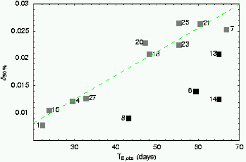
Figure 13: Correlation plot of the median value (square boxes) of $\delta={\frac{D_{\mathrm{os}}-D_{\mathrm{ol}}}{D_{\mathrm{os}}}}$ ($y$–axis) with respect to the measured Einstein time ($x$–axis) of each event. The label identifies the event. The dashed line is the correlation straight line of the cluster of 10 events.

We come now to the discussion of the changes in the microlensing rate induced by the different bar geometry configurations and velocity dispersions, as introduced in Sect. 3.2. The main point to be stressed is that the separation in the two populations for the events already identified is in these cases enhanced. Indeed, the expected characteristics change significantly only for those events along the lines of sight pointing towards the central region: LMC–6, LMC–8 and LMC–14, and, marginally, LMC–1 and LMC–27, as it is the case for the self–lensing optical depth. In Table 2 we report the predicted values for the Einstein time for these 5 events, the changes for the others being at most of $\sim$ 5% (in particular this is the case for the event LMC–13).

event	$T_{\mathrm{E,obs}}$	$T_{\mathrm{E,50\%}}$	$T_{\mathrm{E,50\%}}$	$T_{\mathrm{E,50\%}}$	$\tau\,(10^{-8})$	$\tau\,(10^{-8})$	$\tau\,(10^{-8})$
		coplanar	rotated	shifted	coplanar	rotated	shifted
1	22.3	$64\quad 56$	$76\quad 67$	$64\quad 56$	2.24	3.33	2.23
6	59.5	$55\quad 47$	$57\quad 48$	$62\quad 53$	2.84	3.16	3.90
8	43.1	$48\quad 37$	$53\quad 41$	$51\quad 40$	4.72	5.99	5.58
14	65.0	$51\quad 41$	$60\quad 47$	$56\quad 44$	3.72	5.33	4.53
27	32.8	$67\quad 59$	$75\quad 67$	$69\quad 61$	1.75	2.29	1.94

Table 2: For each MACHO event located within or nearby the bar region, where the variation due to the change in the geometry turn out to be significant, we report for the Einstein time (days): the observed value and the predicted values for the three geometry configurations, bar coplanar with the disk, bar rotated by $40^{\circ}$ with respect to the disk plane and bar shifted by 0.5 kpc along the line of sight towards the observer. The left values are for a velocity dispersion of the bar component of $\sigma_{\mathrm{b}}$=20.2 km/s (as for the disk), whereas the right values are for $\sigma_{\mathrm{b}}$ = 30.0 km/s. We report also the values for the self–lensing optical depth in the direction of the events.

As expected, an increase in the velocity dispersion for the bar component leads to a decrease ($\sim$ 20%) for the predicted values of the Einstein time. For the events LMC–6, LMC–8 and LMC–14 the predicted values just fluctuate around the observed ones, while they remain substantially different for the events LMC–1 and LMC–27. The change in geometry leads, on the contrary, to a rise for the expected values of the Einstein time, at most $\sim$ 10% (the effect being stronger for the rotated bar), for the events LMC–6, LMC–8 and LMC–14. For the event LMC–1 the difference between the observed and the predicted value is further enhanced (up to $\sim$ 16%). This gives further support to the guess that this short duration event is likely to belong to a different population. We note that the two opposite effects on the predicted Einstein time, the decrease linked to the rise of the velocity dispersion opposed to the increase linked to the non coplanar geometry, are actually to be expected as $\Gamma\propto\tau/T$. Analogous considerations emerge from the analysis of the differential rate with respect to $x$ and the mass. In particular, for the mass, we note again two opposite effects. A rise induced by the increase in the velocity dispersion, and a decrease linked to the non coplanar geometry. We observe a maximum increase of $\sim 15$% for the event LMC–14.

To complete this analysis let us make a further point. In the differential rate, Eq. 17, we get an average result for all the possible configurations with lens and source either in the bar or in the disk of the LMC. This is of course coherent with our approach aimed at the study of the statistical properties of the self lensing population as a all. However, it is in principle interesting to notice that the expected characteristics can be actually rather different depending on the configuration. As an example, we consider the event LMC–14, coplanar bar geometry, $\sigma_{\mathrm{b}}=20.2$ km/s. With respect to the previously obtained result, expected median value for the Einstein time $T_{\mathrm{E},50\%}$=51 days, we get a shorter value in the lens-source bar-bar configuration, $\sim 43$ days, a significantly longer value for the disk-disk configuration, $\sim 67$ days, and an intermediate one, $\sim 55$ days, for both mixed configurations, disk-bar and bar-disk. We recall that the observed value for LMC–14 is $T_{\mathrm{E}}$=65 days.

4.4 Expected number of self–lensing events

We compute the “field exposure”, $E_{\mathrm{field}}$, defined, as in Alcock et al. (2000a), as the product of the number of distinct light curves per field by the relevant time span, paying attention to eliminate the field overlaps. Furthermore we calculate the distribution ${\frac{\mathrm{d}\Gamma}{\mathrm{d}T_{\mathrm{E}}}}$ along the line of sight pointing towards the center of each field. In this way we obtain the number of expected events for self lensing, field by field, given by

$$N_{\mathrm{SL,field}}=E_{\mathrm{field}}\int_{0}^{\infty}\,{\frac{\mathrm{d}\Gamma}{\mathrm{d}T_{\mathrm{E}}}}\,{\cal E}(T_{\mathrm{E}})\,\mathrm{d}\,T_{\mathrm{E}}\;,$$ (20)

where ${\cal E}(T_{\mathrm{E}})$ is the detection efficiency.

In Fig. 14 we report in parenthesis the expected number of events in each field we obtain by using the Chabrier exponential IMF. Summing over all fields we find that the expected total number of self–lensing events is $\sim 1.2$, while we would get $\sim 1.3$ with the the double power law IMF, in both cases altogether 1-2 events. Clearly, taking also into account the uncertainties in the parameter used following the van der Marel model for the LMC the actual number could also be somewhat higher but hardly more than twice our estimate. A conclusion we had already reached in Paper I.

We have also computed the influence of the bar geometry and dispersion velocity on the number of expected events. We find at most an increase of $\sim$ 50%, bar rotated and $\sigma_{\mathrm{b}}$= 30 km/s, that gives altogether about 2-3 events.

In conclusion, we have identified, according to their expected characteristics as compared to the observed one, a set of 4 possible events belonging to the self–lensing population (LMC–6, LMC–8, LMC–13 and LMC–14). As already observed, there are some experimental evidences that the LMC–14 is a self–lensing event (Alcock et al. 2001b). If this is true, our prediction of at most 2-3 such events seems thus to indicate that some of the others are more likely not to be due to self lensing.

5 Asymmetry

In this section we consider from a different perspective the issue of the expected near/far asymmetry for events due to lenses located in the LMC or the MW halo. In particular we study, by means of a statistical analysis, the spatial distribution of the events, both in the framework of the van der Marel picture and, for comparison, of the older one. The aim here is to give further support to our main conclusion, namely that self lensing, for which we do not expect any asymmetry in the spatial distribution, can not explain all the detected events.

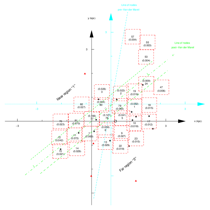
Figure 14: Locations of the 30 MACHO fields with respect to post-Van der Marel LMC geometry (black reference axes) and with respect to pre-Van der Marel LMC geometry (light blue reference axes). Also shown are the locations of the MACHO and EROS microlensing candidates. The distances on the axes are in kpc. For each field, inside brackets, we report the expected number of self–lensing event as discussed in Sect. 4.4.

In Fig. 14, the 30 well-sampled fields analyzed by the MACHO collaboration (red squares), together with the 16 events, are located in a reference frame (black axes) centered in $\alpha_{\mathrm{CM}}=5^{\mathrm{h}}27.6^{\mathrm{m}}$, $\delta_{\mathrm{CM}}=-\,69.87^{\circ}$, J$2000$. We also report the position (triangles) of the microlensing events found by the EROS collaboration (Lasserre et al. 2000) even if we do not consider them in the present analysis.

We divide the LMC field in three regions: a strip centered on the line of nodes and delimited by two parallel straight lines at a distance of $\approx 0.35\,\mathrm{kpc}$ from the line of nodes, and two outer regions, belonging to the closer north-east side and to the farther south-west one. The amplitude of the central strip reflects the uncertainties in the position of the center of mass of carbon stars, as calculated by van der Marel et al. (2002), at one $\sigma$ level. The exclusion of a substantial part of the bar region implies that the following discussion is not affected by the different choices for the bar geometry.

The green dashed–dot line represents the line of nodes with a position angle $\Theta=129.9^{\circ}$ and the two green dashed lines delimit the two outer regions belonging respectively to the near and far part of the LMC.

On the same figure a second reference frame is also reported, according to pre-van der Marel LMC models. The frame (light blue axes) is centered in $\alpha_{\mathrm{gas}}=5^{\mathrm{h}}17.6^{\mathrm{m}}$, $\delta_{\mathrm{gas}}=-\,69^{\circ}02^{\prime}$, J2000 (Kim et al. 1998), and the line of nodes has a position angle $\Theta_{\mathrm{Gyuk}}=170^{\circ}$ (Gyuk et al. 2000). A region of exclusion, similar to the previous one will be considered also in this case, even if not drawn on the figure for clarity sake.

At first glance one observes that the distribution of the events shows a clear near-far asymmetry in the post-van der Marel geometry, namely, they are concentrated along the extension of the bar and in the south-west side of the LMC. On the contrary, the asymmetry is almost completely lost in the pre-van der Marel geometry, where the distribution reflects almost exactly the different weights of the observed fields in the two half planes, as we will show in the following.

The little empty circle in the field number 5 locates the position of the baricenter of the 16 MACHO events, whose coordinates in the post-van der Marel reference frame are (0.96 kpc, – 0.02 kpc).

5.1 Near-far asymmetry of the observed microlensing events in the LMC

In order to give a quantitative analysis of the near–far asymmetry, we will concentrate on the MACHO observed fields (and the corresponding observed events) in the outer regions located on the opposite sides of the line of the nodes and external to the dashed lines, which, at a good confidence level, belong respectively to the near and far part of the galaxy.

As a first point we determine the fraction of the MACHO fields included respectively in the north-east closer region “1” and in the south-west farther region “2”, and we calculate in each the quantities $\Sigma_{1}$ and $\Sigma_{2}$, defined as the sum of the product of star number pro field, times the corresponding observation time, where we count only once the stars in the intersecting part of the fields. The ratio $\Sigma_{i}/(\Sigma_{1}+\Sigma_{2})$ gives us the probability $p_{i}$ that a microlensing event would fall in the first or second region, respectively. Let us note that the probability scheme so defined depends only on the global observation strategy in the near and far region (fields distribution and observation time). We find $p_{1}\approx 0.31$ in the case of the post-van der Marel LMC geometry, and $\tilde{p}_{1}\approx 0.48$ for the pre-van der Marel LMC geometry.

We are interested in testing whether the observed events support the modelled probability schemes. The Pearson chi-square statistic ${\cal A}_{N}$ provides a non parametric test for the comparison:

$${\cal A}_{N}=\sum_{i=1}^{2}{{(n_{i}-Np_{i})^{2}}\over Np_{i}}\leavevmode\nobreak\ ,$$ (21)

where $n_{i}$ are the events falling in the $i$-region, and $N=n_{1}+n_{2}$. ${\cal A}_{N}$ is approximately distributed as chi-square with one degree of freedom. Small values of ${\cal A}_{N}$ tend to support the null hypothesis that the $p_{i}$ match the measured distribution.

In the post-van der Marel geometry we get, respectively, 1 and 9 observed events in regions “1” and “2”, and then

$${{\cal A}_{10}}=2.11.$$

On the contrary, in the case of pre-van der Marel geometry, we obtain:

$${\tilde{\cal A}_{12}}=0.22,$$

starting from a set of 5 and 7 observed events.

In the pre-van der Marel geometry ${{\cal A}_{N}}$ gets a value near to zero. At the confidence level of $\simeq 64\%$ the null hypothesis that the events distribution reflects almost exactly the weights of the two regions has to be accepted. This implies that the distribution of the lenses should be almost homogeneous along the lines of sight through the different regions of the LMC.

On the contrary, in the post-van der Marel geometry ${{\cal A}_{N}}$ assumes a value far enough from zero. At the confidence level of $\simeq 85\%$ the null hypothesis must be rejected. This means that the observed asymmetry is greater than the one expected simply on the basis of the observational strategy.

We are aware that these results have to be treated with caution inasmuch as the number of events is small. However, we note that the observed near–far asymmetry is coherent with that induced by the inclination of the LMC disk already discussed, looking at the optical depth, in Sect. 4.1.

6 An improved Gould inequality

Gould (1995) ingenious calculation provides two inequalities (Eq. (2.8) and Eq. (3.3) of his paper), the second one involving the Jeans equation and the virial theorem, which allow, in some cases, a quick evaluation of an upper limit to the self–lensing optical depth along a line of view through the center of a galaxy. In particular this was applied to the LMC disk, in order to exclude the Sahu (1994) hypothesis that the observed optical depth could be fully explained by self lensing.

Our aim here is to obtain an improved version of Gould inequality, and, at the same time, clarify its limits of applicability. We start from Eq. (10) and consider the case of a line of view passing through the center of the LMC.

Let us assume that the lens mass density $\rho_{\mathrm{l}}$ be a function of an homogeneous polynomial of degree $n_{\mathrm{l}}$ in the variables $(\xi,\,\eta,\,\zeta)$ of the reference frame defined in Sect. 3.1, and analogously that the star mass density $\rho_{\mathrm{s}}$ be a function of an homogeneous polynomial of degree $n_{\mathrm{s}}$. Let us also denote with $z$ the current coordinate along the line of view through the center of the LMC disk, which we assume as the origin of the $z$–coordinate, and with $i$ the disk inclination angle. Keeping in mind that for points belonging to a line of view passing through the center it results:

$$\xi= 0$$

$$\eta= z\sin i$$

$$\zeta= z\cos i$$

we can write for the lens density distribution

$$\rho_{l}[0,\,\eta,\,\zeta] =\rho_{l}\left[\sum_{k=0}^{n}\,c_{k,n-k}^{(\mathrm{l})}\,\left({\frac{\eta}{\eta_{\mathrm{l},0}}}\right)^{k}\,\left({\frac{\zeta}{\zeta_{\mathrm{l},0}}}\right)^{n-k}\right]$$ (22)

$$=\rho_{\mathrm{l}}\left[\gamma_{\mathrm{l}}(i)\,\left({\frac{z}{\zeta_{\mathrm{l},0}}}\right)^{n}\right]$$

with

$$\gamma_{\mathrm{l}}(i)=\sum_{k=0}^{n}\,c_{k,n-k}^{(\mathrm{l})}\,\left({\frac{\eta_{\mathrm{l,}0}}{\zeta_{\mathrm{l},0}}}\right)^{k}\sin^{k}(i)\,\cos^{n-k}(i)$$ (23)

and $\eta_{\mathrm{l},0}$, $\zeta_{\mathrm{l},0}$ the scale lengths of the lenses density distribution. Analogous expressions can be written for the star density distribution, changing properly the suffix “l” with “s”.

From now on we follow Gould (1995), and put $D_{\mathrm{ol}}=d+z$ and $D_{\mathrm{os}}=d+w$, where $d$ is the distance, along the line of view, from the observer to the center of the disk. Taking into account that

$${\frac{d+z}{d+w}}<1,$$

we obtain the following inequality for the optical depth:

$$\tau\leq {\frac{4\pi G}{c^{2}}}\int_{-t}^{t}\mathrm{d}w\,\rho_{\mathrm{s}}\left[\gamma_{\mathrm{s}}(i)\,\left({\frac{w}{\zeta_{\mathrm{s},0}}}\right)^{n_{\mathrm{{\mathrm{s}}}}}\right]\cdot$$ (24)

$$\cdot{\frac{\int_{-d}^{w}\mathrm{d}z\,(w-z)\,\rho_{\mathrm{l}}\left[\gamma_{\mathrm{l}}(i)\,\left({\frac{z}{\zeta_{\mathrm{l},0}}}\right)^{n_{\mathrm{l}}}\right]}{\int_{-t}^{t}\mathrm{d}w\,\rho_{\mathrm{s}}\left[\gamma_{\mathrm{s}}(i)\,\left({\frac{w}{\zeta_{\mathrm{s},0}}}\right)^{n_{\mathrm{s}}}\right]}},$$

where $t$ is the the LMC tidal radius.

We now integrate by part twice, a first time obtaining:

$$\tau\leq{\frac{4\pi G}{c^{2}}}\int_{-t}^{t}\mathrm{d}w\,\rho_{\mathrm{s}}\left[\gamma_{\mathrm{s}}(i)\,\left({\frac{w}{\zeta_{\mathrm{s},0}}}\right)^{n_{\mathrm{s}}}\right]\cdot$$

$$\cdot{\frac{\int_{-d}^{w}\,\mathrm{d}z\,\int_{-d}^{z}\mathrm{d}u\,\rho_{l}\left[\gamma_{\mathrm{l}}(i)\,\left({\frac{u}{\zeta_{\mathrm{l},0}}}\right)^{n_{\mathrm{l}}}\right]}{\int_{-t}^{t}\mathrm{d}w\rho_{\mathrm{s}}\,\left[\gamma_{\mathrm{s}}(i)\,\left({\frac{w}{\zeta_{\mathrm{s},0}}}\right)^{n_{\mathrm{s}}}\right]}}$$ (25)

and a second time obtaining:

$$\tau\leq {\frac{4\pi G}{c^{2}}}\int_{-d}^{t}\mathrm{d}z\,\rho_{\mathrm{l}}\left[\gamma_{\mathrm{l}}(i)\,\left({\frac{z}{\zeta_{\mathrm{l},0}}}\right)^{n_{\mathrm{l}}}\right]\,\cdot$$ (26)

$$\cdot\left\{\int_{-t}^{t}\,\mathrm{d}w\,{\frac{\int_{-d}^{w}\mathrm{d}z\,\rho_{\mathrm{l}}\left[\gamma_{\mathrm{l}}(i)\,\left({\frac{z}{\zeta_{\mathrm{l},0}}}\right)^{n_{\mathrm{l}}}\right]}{\int_{-d}^{t}\mathrm{d}z\,\rho_{\mathrm{l}}\left[\gamma_{\mathrm{l}}(i)\,\left({\frac{z}{\zeta_{\mathrm{l},0}}}\right)^{n_{\mathrm{l}}}\right]}}\right.\cdot$$

$$\qquad\left.\left(1-{\frac{\int_{-t}^{w}\mathrm{d}z\,\rho_{\mathrm{s}}\left[\gamma_{\mathrm{s}}(i)\,\left({\frac{z}{\zeta_{\mathrm{s},0}}}\right)^{n_{\mathrm{s}}}\right]}{\int_{-t}^{t}\,\rho_{\mathrm{s}}\left[\gamma_{\mathrm{s}}(i)\,\left({\frac{z}{\zeta_{\mathrm{s},0}}}\right)^{n_{\mathrm{s}}}\right]\,\mathrm{d}z}}\right)\right\}.$$

In case of self lensing $\rho_{\mathrm{s}}$ and $\rho_{\mathrm{l}}$ coincide. Moreover, for distances higher than the tidal radius of the LMC, the star mass density $\rho_{\mathrm{s}}=0$, and we can move the lower integration limit from $-t$ or $-d$ to $-\infty$, and the upper from $t$ to $+\infty$. We are considering a line of view passing through the center of the LMC, therefore we can use the symmetry property of the mass density distributions with respect to change of sign of the parameter $z$ and we obtain:

$$\tau\leq {\frac{\pi G}{c^{2}}}\int_{-\infty}^{\infty}\mathrm{d}z\,\rho_{\mathrm{s}}\left[\gamma_{\mathrm{s}}(i)\,\left({\frac{z}{\zeta_{\mathrm{s},0}}}\right)^{n_{\mathrm{s}}}\right]\,\cdot$$ (27)

$$\cdot\int_{-\infty}^{\infty}\mathrm{d}v\,\left[1-F_{s}^{2}(v)\right],$$

where

$$F_{\mathrm{s}}(v)={\frac{2\int_{0}^{v}\mathrm{d}z\,\rho_{\mathrm{s}}\left[\gamma_{\mathrm{s}}(i)\,\left({\frac{z}{\zeta_{\mathrm{s},0}}}\right)^{n_{\mathrm{s}}}\right]}{\int_{-\infty}^{\infty}\mathrm{d}z\,\rho_{\mathrm{s}}\left[\gamma_{\mathrm{s}}(i)\,\left({\frac{z}{\zeta_{\mathrm{s},0}}}\right)^{n_{\mathrm{s}}}\right]}}.$$ (28)

A suitable change of variables gives:

$$\tau \leq {\frac{2\,\pi\,G\,\zeta_{\mathrm{s},0}^{2}}{c^{2}}}\left[\gamma_{\mathrm{s}}(i)\right]^{-{\frac{2}{n_{\mathrm{s}}}}}\cdot$$ (29)

$$\int_{-\infty}^{\infty}\,\rho_{\mathrm{s}}\left(u^{n_{\mathrm{s}}}\right)\,\mathrm{d}u\,\int_{0}^{\infty}\left[1-F_{\mathrm{s}}^{2}(v)\right]\,\mathrm{d}v,$$

where

$$F_{\mathrm{s}}(v)={\frac{2\int_{0}^{v}\,\rho_{\mathrm{s}}\left(u^{n_{\mathrm{s}}}\right)\,\mathrm{d}u}{\int_{-\infty}^{\infty}\,\rho_{\mathrm{s}}\left(u^{n_{\mathrm{s}}}\right)\,\mathrm{d}u}}$$ (30)

and the integrations are now made on adimensional variables.

Let us observe that the inequality (29) can be applied for any inclination angle $i$ of the disk plane, not only for $i<<\pi/2$, as in Gould (1995), namely, we have no divergence problem for $i\rightarrow\pi/2$. For instance, in the case of a double exponential disk, with scale lengths respectively equal to $R_{\mathrm{d}}$ and $\zeta_{\mathrm{d}}$, we obtain:

$$\tau\leq {\frac{2\,\pi\,G\,\zeta_{\mathrm{d}}^{2}}{c^{2}}}{\frac{1}{\left[{\cos(i)}+{\frac{\zeta_{\mathrm{d}}}{R_{\mathrm{d}}}}\sin(i)\right]^{2}}}\,\int_{-\infty}^{\infty}\,\rho_{\mathrm{s}}\left(u\right)\,\mathrm{d}u\,\cdot$$ (31)

$$\int_{0}^{\infty}\left[1-F_{\mathrm{s}}^{2}(v)\right]\,\mathrm{d}v.$$

Or in the case of a gaussian profile of the mass density distribution for the LMC bar, as in Gyuk et al. (2000), with scale length $\eta_{\mathrm{b}}$ along the axis bar and $\zeta_{\mathrm{b}}$ in the orthogonal section, we obtain:

$$\tau\leq {\frac{2\,\pi\,G\,\zeta_{\mathrm{b}}^{2}}{c^{2}}}{\frac{1}{{\cos^{2}(i)}+\left({\frac{\zeta_{\mathrm{b}}}{\eta_{\mathrm{b}}}}\right)^{2}\sin^{2}(i)}}\,\int_{-\infty}^{\infty}\,\rho_{\mathrm{s}}\left(u^{2}\right)\,\mathrm{d}u\,\cdot$$ (32)

$$\int_{0}^{\infty}\left[1-F_{\mathrm{s}}^{2}(v)\right]\,\mathrm{d}v.$$

For a bar having boxy contours and sharp edges as in the paper of Zhao & Evans (2000), parameterized by an exponential profile with a fourth degree polynomial at the exponent, with scale length $\eta_{\mathrm{b}}$ along the axis bar and $\zeta_{\mathrm{b}}$ in the orthogonal section, we obtain:

$$\tau\leq {\frac{2\,\pi\,G\,\zeta_{\mathrm{b}}^{2}}{c^{2}}}{\frac{1}{\sqrt{{\cos^{4}(i)}+\left({\frac{\zeta_{\mathrm{b}}}{\eta_{\mathrm{b}}}}\right)^{4}\sin^{4}(i)}}}\,\int_{-\infty}^{\infty}\,\rho_{\mathrm{s}}\left(u^{4}\right)\,\mathrm{d}u\,\cdot$$ (33)

$$\int_{0}^{\infty}\left[1-F_{\mathrm{s}}^{2}(v)\right]\,\mathrm{d}v.$$

Eq. (29) is the improved version of Eq. (2.8) of Gould (1995).

Proceeding in the same way as in Gould (1995), we obtain the second Gould inequality, relating the optical depth with the mass-weighted velocity dispersion.

$$\tau\leq 2{\frac{<v^{2}>}{c^{2}}}\left[\gamma_{\mathrm{s}}(i)\right]^{-{\frac{2}{n_{\mathrm{s}}}}}.$$ (34)

Let us note that these inequalities are based on two properties:

• that the star density be a function of an homogeneous polynomial of the variables, of any degree;

• that the line of view pass through the center, in such a way we can use the symmetry by reflection of the mass density distributions.

Let us note, moreover, that the inequalities (29) and (34) can not be applied to the model of the LMC disk and bar we assumed in this paper, because the first property, that of homogeneity, is lacking.

It is therefore useful to derive a more general inequality, applicable to all kinds of density distribution.

6.1 A more general inequality

We start from equation (6), but we relax the hypothesis that the mass density distribution be a function of an homogeneous polynomial:

$$\tau\leq{\frac{4\pi G}{c^{2}}}{\frac{\int_{-t}^{t}\mathrm{d}w\,\rho_{\mathrm{s}}(w)\int_{-d}^{w}\mathrm{d}z\,\int_{-d}^{z}\mathrm{d}u\,\rho_{\mathrm{l}}(u)}{\int_{-t}^{t}\mathrm{d}w\,\rho_{\mathrm{s}}\,(w)}}.$$ (35)

Let us divide in three part the triangular region of integration in the plane $(u,z)$, delimited by the bisector of the first and third quadrant, by the parallel to the $u$-axis of equation $z=w$ and by the parallel to $z$–axis of equation $u=-d$: the first region is constituted by the triangle delimited by the bisector, the line $u=-d$ and the $u$–axis; the second by the rectangle delimited by the $u$–axis, the $z$–axis and the lines of equation $z=w$ and $u=-d$; the third by the triangle delimited by the bisector, the z-axis and the line of equation $z=w$. Let us remember that $w$ can assume any value between $-t$ and $t$. In this way, the right hand side of Eq. (35) is given by the sum of three terms:

$${\frac{4\,\pi\,G}{c^{2}}}\left\{\int_{-d}^{0}\mathrm{d}z\,\int_{-d}^{z}\mathrm{d}u\,\,\rho_{\mathrm{l}}(u)\,+\,\int_{-d}^{0}\mathrm{d}z\,\rho_{\mathrm{l}}(z){\frac{\int_{-t}^{t}\mathrm{d}w\,w\,\rho_{\mathrm{s}}(w)}{\int_{-t}^{t}\mathrm{d}w\,\rho_{\mathrm{s}}(w)}}\right.$$

$$\left.+\,{\frac{\int_{-t}^{t}\mathrm{d}w\,\rho_{\mathrm{s}}(w)\int_{0}^{w}\mathrm{d}z\,\int_{0}^{z}\mathrm{d}u\,\rho_{\mathrm{l}}(u)}{\int_{-t}^{t}d\mathrm{w}\,\rho_{\mathrm{s}}\,(w)}}\right\}.$$ (36)

After an integration by part, the first term becomes

$${\frac{4\,\pi\,G}{c^{2}}}\int_{0}^{d}\mathrm{d}z\,z\,\rho_{\mathrm{s}}(-z);$$

the second term is null, thanks to the symmetry by reflection of $\rho_{\mathrm{s}}(z)$. As regard the third term we observe that for any $z$ belonging to the interval $(-t,t)$ it always results

$$\int_{0}^{z}\mathrm{d}u\,\rho_{\mathrm{l}}(u)\leq\int_{0}^{t}\mathrm{d}u\,\rho_{\mathrm{l}}(u)$$

and therefore

$${\frac{\int_{-t}^{t}\mathrm{d}w\,\rho_{\mathrm{s}}(w)\int_{0}^{w}\mathrm{d}z\,\int_{0}^{z}\mathrm{d}u\,\rho_{\mathrm{l}(}u)}{\int_{-t}^{t}\mathrm{d}w\,\rho_{\mathrm{s}}\,(w)}}\leq \int_{-t}^{t}\mathrm{d}w\,w\,\rho_{\mathrm{s}}(w)\,\cdot$$ (37)

$${\frac{\int_{0}^{t}\mathrm{d}u\,\rho_{\mathrm{l}}(u)}{\int_{-t}^{t}\mathrm{d}w\,\rho_{\mathrm{s}}\,(w)}}.$$

This way we obtain that also the third term is less than zero. In conclusion we obtain the searched inequality for the optical depth, valid for any mass density distribution of lenses. In particular for lenses in the galactic halo we obtain:

$$\tau_{\mathrm{GH}}\leq{\frac{4\,\pi\,G}{c^{2}}}\int_{0}^{d}\mathrm{d}z\,z\,\rho_{\mathrm{l,GH}}(-z),$$ (38)

for lenses in the LMC halo we obtain

$$\tau_{\mathrm{LMCH}}\leq{\frac{4\,\pi\,G}{c^{2}}}\int_{0}^{t}\mathrm{d}z\,z\,\rho_{\mathrm{l,LMCH}}(z),$$ (39)

and for self lensing we obtain

$$\tau_{\mathrm{SL}}\leq{\frac{4\,\pi\,G}{c^{2}}}\int_{0}^{t}\mathrm{d}z\,z\,\rho_{\mathrm{s}}(z).$$ (40)

Applying this last inequality to the LMC mass density distribution used in our (coplanar) model we find

$$\tau_{\mathrm{SL}}\leq 6\times 10^{-8},$$

only about 20% higher than the calculated value.

Notice that on the right hand side of the inequality (38) $\rho_{\mathrm{l,GH}}(-z)\neq\rho_{\mathrm{l,GH}}(z),$ since the galactic halo density is not symmetric with respect to the LMC center. The inequality, therefore, cannot be obtained by a trivial dropping of the factor $(1-z)$ in the integrand of the expression defining the galactic halo optical depth.

7 Summary

The great interest in the location of the observed microlensing events towards the LMC is motivated by the need to give an answer to the question of their nature. Namely, whether (or not) all the events can be attributed to known (luminous) populations, so to exclude (or not) the possibility for a dark component in the halo in the form of MACHOs.

In this paper we are mainly concerned with the possible self–lensing origin of the observed microlensing events. In particular we have considered the results of the MACHO survey. We use the recent picture of the LMC disk given by van der Marel et al. (2002), and we explore different geometries for the bar component, as well as a reasonable range for the velocity dispersion for the bar population.

One interesting feature, essentially linked to the assumed disk geometry, is an evident near–far asymmetry of the optical depth for lenses located in the LMC Halo (this is not expected, with the possible exception of the inner region, for the self–lensing population). Indeed, similarly to the case of M31 (Crotts 1992; Jetzer 1994), and as first pointed out by Gould (1993), since the LMC disk is inclined, the optical depth is higher along lines of sight passing through larger portions of the LMC halo. We show that such a spatial asymmetry, beyond the one expected from the observational strategy alone, is indeed present in the observed events. With the care suggested by the small number of detected events on which this analysis is based, this can be looked at, as yet observed by Gould (1993), as a signature of the presence of an extended halo around the LMC.

In the central region the microlensing signatures are strongly dependent on the assumed bar geometry. In particular, we have studied the variation (that can be as large as 50%) in the self–lensing optical depth due to the different geometry of the bar. However, the available data do not allow us to meaningfully explore in more detail this aspect.

As a further step in our analysis, we have studied the microlensing rate. Keeping in mind Evans & Kerins (2000) observation that the timescale distribution of the events and their spatial variation across the LMC disk offers possibilities of identifying the dominant lens population, we have carefully characterized the ensemble of observed events under the hypothesis that all of them do belong to the self–lensing population. Through this analysis we have been able to identify a large subset of events that can not be accounted as part of this population. The introduction of a non coplanar bar component with respect to the disk turns out to enhance this result. Again, the small amount of events at disposal does not yet allow us to draw sharp conclusions, although, the various arguments mentioned above are all consistent among them and converge quite clearly in the direction of excluding self lensing as being the major cause for the events.

Once more observations will be available, as will hopefully be the case with the SuperMacho experiment under way (Stubbs et al. 2002), the use of the above outlined methods can bring to a definitive answer to the problem of the location of the MACHOs and thus also to their nature.

——————————————————————

References

- Alcock et al. (1997) Alcock, C., Allsman, R.A., Alves, D.R., et al. 1997, ApJ, 486, 697
- Alcock et al. (2000a) Alcock, C., Allsman, R.A., Alves, D.R., et al. 2000a, ApJ, 542, 281
- Alcock et al. (2000b) Alcock, C., Allsman, R.A., Alves, D.R., et al. 2000b, ApJ, 541, 270
- Alcock et al. (2001a) Alcock, C., Allsman, R.A., Alves, D.R., et al. 2001a, Nature, 414, 617
- Alcock et al. (2001b) Alcock, C., Allsman, R.A., Alves, D.R., et al. 2001b, ApJ, 552, 259
- Alcock et al. (2001c) Alcock, C., Allsman, R.A., Alves, D.R., et al. 2001c, ApJ, 552, 582
- Alves & Nelson (2000) Alves, D.R., & Nelson C.A., 2000, ApJ, 542, 789
- Aubourg et al. (1999) Aubourg, E., Palanque-Delabrouille N., Salati, P. et al. 1999, A&A, 347, 850
- Chabrier (2001) Chabrier, G. 2001, ApJ, 554, 1274
- Cioni et al. (2000) Cioni, M.-R.L., Loup, C., Habing, H.J., et al. 2000, A&AS, 144, 235
- Crotts (1992) Crotts, A.P.S. 1992, ApJ, 399, L43
- Cutri et al. (2000) Cutri, R.M., Skrutskie, M.F., Van Dyk, S., et al. 2000, 2MASS Second Incremental Data Release
- Drake et al. (2004) Drake, A.J., Cook, K.H., & Keller, S.C., astro-ph/0404285
- de Rújula et al. (1991) de Rújula, A., Jetzer, Ph., & Massó, E. 1991, MNRAS, 250, 348
- de Rújula et al. (1995) de Rújula, A., Giudice, G.F., & Mollerach, S., & Roulet, E. 1995, MNRAS, 275, 545
- Evans & Kerins (2000) Evans, N.W., & Kerins, E. 2000, ApJ, 529, 917
- Gerhard (1993) Gerhard, O.E. 1993, MNRAS, 265, 213
- Gould (1993) Gould, A. 1993, ApJ, 404, 451
- Gould (1995) Gould, A. 1995, ApJ, 441, 77
- Gould (2004) Gould, A. 2004, ApJ, 606, 319
- Griest (1991) Griest K. 1991, ApJ, 366, 412
- Gyuk et al. (2000) Gyuk, G., Dalal, N. & Griest, K. 2000, ApJ, 535, 90
- Jetzer (1994) Jetzer, Ph. 1994, A&A, 286, 426
- (24) Jetzer, Ph., Mancini, L. & Scarpetta, G. 2002, A&A, 393, 129 (Paper I)
- Kim et al. (1998) Kim, S., Staveley-Smith, L., Dopita, M.A., et al. 1998, ApJ, 503, 674
- Lasserre et al. (2000) Lasserre, T., Afonso, C., Albert J.N., et al. 2000, A&A, 355, L39
- Milsztajn (2003) Milsztajn, A. 2003, Private communication
- Nikolaev et al. (2004) Nikolaev, S., Drake, A.J., Keller, S.C., et al. 2004, ApJ, 601, 260
- Olsen & Salyk (2002) Olsen, K.A.G., & Salyk, C. 2002, AJ, 124, 2045
- Primack et al. (1988) Primack, J.R., Seckel, D. & Sadoulet, B. 1988, Ann. Rev. Nucl. Part. Sci., 38, 751
- Sahu (1994) Sahu, K.C. 1994, PASP, 106, 942
- Stubbs et al. (2002) Stubbs, C. W., Rest, A., Miceli, A., et al. 2002, BAAS, 201, #78.07
- van der Marel & Franx (1993) van der Marel, R.P., & Franx, M. 1993, ApJ, 407, 525
- van der Marel & Cioni (2001) van der Marel, R.P., & Cioni, M.R. 2001, AJ, 122, 1807
- van der Marel (2001) van der Marel, R.P. 2001, AJ, 122, 1827
- van der Marel et al. (2002) van der Marel, R.P., Alves, D.R., Hardy, E., & Suntzeff, N.B. 2002, AJ, 124, 2639
- von Hippel et al. (2003) von Hippel, T., Sarajedini, A., Ruiz, M.T. 2003, ApJ, 595, 794
- Weinberg (2000) Weinberg, M.D. 2000, ApJ, 532, 922
- Weinberg & Nikolaev (2001) Weinberg, M.D., & Nikolaev, S. 2001, ApJ, 548, 712
- Wu (1994) Wu, X. P. 1994, ApJ, 435, 66
- Zasov & Khoperskov (2002) Zasov, A. V., & Khoperskov, A. V. 2002, Astron. Reports, 4603, 173
- Zhao & Evans (2000) Zhao, H.S., & Evans, N.W. 2000, ApJ, 545, L35