Radio emission and particle acceleration in plerionic supernova remnants

Plerionic supernova remnants exhibit radio emission with remarkably flat spectral indices ranging from $\alpha=0.0$ to $\alpha=-0.3$. The origin of very hard particle energy distributions still awaits an explanation, since shock waves generate particle distributions with synchrotron spectra characterized by $\alpha\leq-0.5$. Acceleration of high energy leptons in magnetohydrodynamic turbulence instead may be responsible for the observed hard spectra. This process is studied by means of relativistic test particle calculations using electromagnetic fields produced by three-dimensional simulations of resistive magnetohydrodynamical turbulence. The particles receive power-law energy spectra $N(\gamma)\propto\gamma^{-s}$ with $s$ ranging from $1.2$ to $1.6$, i.e. particle spectra that are required to explain the radio emission of plerions.

1 Introduction

Filled-center supernova remnants (SNR), or plerions exhibit flat radio spectra, with power-law indices $0\leq\alpha\leq 0.3$ (for $S_{\nu}\propto\nu^{-\alpha}$) (Weiler & Panagia weiler1 (1978); Weiler & Shaver weiler2 (1978)). Such spectra require energy distributions of the electrons $N(\gamma)\propto\gamma^{-s}$ with $s=1+2\alpha$ be in the range $1\leq s\leq 1.6$. The flatness of their radio spectra distinguishes plerions from a typical shell-type SNR with a mean $\alpha\sim 0.5$ implying $N(\gamma)\propto\gamma^{-2}$ (e.g. Green 1991). The origin of relativistic electrons responsible for these unusual radio spectra of plerions is not yet understood (e.g. Green green2 (1992); Woltjer et al. woltjer (1997); Arons arons (1998)).

Although the many details of the nature and structure of plerions are still unclear (see Arons arons (1998); Salvati et al. salvati (1998); Bandiera bandiera1 (2002) for reviews) there is a consensus on the following scenario: Plerions are expanding bubbles, filled with magnetic fields and relativistic leptons. Both components are continuously supplied to the nebula by some central source, i.e. by a rotating neutron star in form of a strongly magnetized wind whose energy is at least partially dissipated in termination shock waves (Kennel & Coroniti 1984a ; 1984b ; Galant & Arons galant (1994)).

Arons (arons (1998)) discussed the difficulties of particle acceleration in plerions in great detail. With respect to prototypic Crab nebula he pointed out that the emission at high frequencies (from the optical towards X- and $\gamma$-rays) diagnoses the coupling physics today since the synchrotron loss times of the high energy particles are significantly smaller than the lifetime of the nebula. The radio emission instead measures the integral of the pulsars input over the entire history of the nebula - most of the stored relativistic energy is in magnetic fields and radio emitting particles (about $10^{50}ergs$). Arons noted that averaged over the whole nebula, the radio emitting spectrum has the form $N(\gamma)\propto\gamma^{-1.5}$, $10^{2.5}\leq\gamma\leq 10^{4}$ based on the detailed spectral index maps by Bietenholz & Kronberg (bietenholz (1992)) which show the particle distribution to be remarkably homogeneous. The origin for this energy distribution is not clear since the wind termination shock wave models do not yield power laws flatter than $N(\gamma)\propto\gamma^{-2}$ at energies small compared to $\gamma\sim 10^{6}$. Arons speculated that some additional acceleration physics by magnetohydrodynamic (MHD) waves may have to be included.

Bandiera et al. (bandiera2 (2002)) mapped the Crab Nebula at 230 GHz and compared it 1.4 GHz map. The spectral index in the inner region at 230 GHz is flatter (by $\sim 0.05$) than in the rest of the nebula. Furthermore they found a steepening of the spectrum at the places of radio emitting filaments, concluding that the magnetic field strengths in the filaments is higher than in the surrounding nebula. Some evidence for in-situ acceleration in the Crab nebula has been collected by the radio observations of Bietenholtz, Frail & Hester (2001).

It is the aim of our contribution to show that resistive magnetohydrodynamical fluctuations excited to a highly turbulent level accelerate test particles to energy distributions with power law indices $1\leq s\leq 1.6$ being in good agreement with the radio observations of plerions. We also show that an increase in particle density as can expected for the filaments lead to a steepening of the particle spectrum. Given the fact, that central sources energize the nebula, thereby exciting strong MHD fluctuations we think that our simulations may shed some light on the probably necessary additional acceleration physics as speculated by Arons (arons (1998)).

In the next section we describe the MHD simulations. Section 3 contains the results of relativistic particle simulations including radiative synchrotron losses and finally we discuss our findings in Section 4

2 Reconnective MHD turbulence

Pulsars permanently power their environment by radiation and, in particular, pulsar plasma winds. In fact, in the case of the Crab nebula the permanent energy input by plasma flow is about $10^{38}$ erg/s. This plasma flow encounters the termination shock at radius $R_{\mathrm{s}}\approx 10^{17}\mathrm{cm}$ where it gets decelerated and leptons are accelerated to ultra-relativistic energies. Most of their synchrotron radiation is emitted in the optical to $\gamma$-ray band. The presence of this termination shock is accompanied by strong excitation of Alfvén waves which are expected to excite strong MHD turbulence in the pulsar’s nebula (Kronberg et al. kronberg (1993)). In this picture the size of the turbulence cells in the nebula is limited by $R_{\mathrm{s}}$. The projected magnetic field within the Crab nebula was found to have a coherence length of about $10^{16}\,cm$ (Bietenholz & Kronberg 1992). Kronberg et al (1993) suggested that the fact that this length scale is close to the inner shock radius $R_{\mathrm{s}}$, may be more than coincidental. Laboratory studies of turbulent flows have revealed the existence of persistence structures, which are advected in the flow and exhibit sizes comparable to the source size (Hussein hussein1 (1983, 1986)). In other words, the source of turbulence within a supernova remnant is given by a shock wave, like in the Crab nebula, the spatial scale of the shock is the maximum length scale for turbulence within the nebula. To be precise, in the Crab nebula the characteristic size of the turbulence should be smaller than $10^{17}\mathrm{cm}$.

The associated MHD turbulence can be numerically generated by means of the so-called Orszag-Tang turbulence (Orszag & Tang orszag (1979)). The Orszag-Tang initial condition is a generic way to excite turbulence in a magnetized plasma and is given by the non-linear interaction of Alfvén waves which are MHD eigenmodes of a magnetized fluid e.g.,

$$B_{x} = -B_{0}\sin\left[2\pi(y-y_{{\rm min}})/(y_{{\rm max}}-y_{{\rm min}})\right]$$ (1)

$$\sin\left[2\pi(z-z_{{\rm min}})/(z_{{\rm max}}-z_{{\rm min}})\right]$$

$$B_{y} = B_{0}\sin\left[4\pi(x-x_{{\rm min}})/(x_{{\rm max}}-x_{{\rm min}})\right]$$ (2)

$$\sin\left[2\pi(z-z_{{\rm min}})/(z_{{\rm max}}-z_{{\rm min}})\right]$$

$$B_{z} = B_{0}\sin\left[4\pi(x-x_{{\rm min}})/(x_{{\rm max}}-x_{{\rm min}})\right]$$ (3)

$$\sin\left[2\pi(y-y_{{\rm min}})/(y_{{\rm max}}-y_{{\rm min}})\right]$$

$$v_{x} = -v_{0}\sin\left[2\pi(y-y_{{\rm min}})/(y_{{\rm max}}-y_{{\rm min}})\right]$$ (4)

$$\sin\left[2\pi(z-z_{{\rm min}})/(z_{{\rm max}}-z_{{\rm min}})\right]$$

$$v_{y} = v_{0}\sin\left[2\pi(x-x_{{\rm min}})/(x_{{\rm max}}-x_{{\rm min}})\right]$$ (5)

$$\sin\left[2\pi(z-z_{{\rm min}})/(z_{{\rm max}}-z_{{\rm min}})\right]$$

$$v_{z} = 0$$ (6)

The amplitudes are chosen as $B_{0}=5.5\times 10^{-3}\;\mathrm{G}$ and $v_{0}=0.05$, $0.016$, $0.005$, $0.0016$, $0.0005$, $0.00016\;\mathrm{c}$ for the six different test particle runs discussed in section 3.

The nonlinear interaction of the Alfvénic perturbations result in almost homogeneous turbulence. We use periodic boundary conditions in all directions and a numerical box given by $x_{\rm min},y_{\rm min},z_{\rm min}=-0.5\times 10^{16}\;\mathrm{cm}$ and $x_{\rm max},y_{\rm max},z_{\rm max}=0.5\times 10^{16}\;\mathrm{cm}$ with a resolution of $101^{3}$ grid points.

We model this kind of turbulence by means of a well approved resistive compressible 3D MHD code (Otto otto (1990)). It integrates the balance equations that govern the macroscopic low-frequency dynamics which read

$${\partial\rho\over\partial t}+\nabla\cdot\left(\rho{\bf v}\right)=0$$ (7)

$${\partial\rho{\bf v}\over\partial t}+\nabla\cdot\left(\rho{\bf v}{\bf v}\right)=-\nabla p+\frac{1}{4\pi}(\nabla\times{\bf B})\times{\bf B}$$ (8)

$${{\partial p}\over{\partial t}}=-{\bf{v}}\cdot\nabla p-\gamma p\nabla\cdot{\bf{v}}+\left(\gamma-1\right)\eta\left(\nabla\times\bf{B}\right)^{2}$$ (9)

$$\frac{1}{c}{\partial{\bf B}\over\partial t}=\nabla\times\frac{1}{c}\left({\bf v}\times{\bf B}\right)-\frac{c}{4\pi}\nabla\times\left(\eta\nabla\times{\bf B}\right)$$ (10)

where $\rho$, ${\bf v}$, $p$, and ${\bf B}$ denote the mass density, bulk velocity, thermal pressure, and the magnetic field. By $\eta$ the resistivity is denoted.

Reconnection is allowed due to a microturbulent resistivity which is modeled in a current dependent way. The motivation for this kind of resistivity is the following: In the highly turbulent almost ideal plasma of the nebula collisional resistivity is negligible. Rather a wide variety of micro-instabilities driven by electric currents is responsible for localized dissipation. For strong turbulence the amplitude of the resistivity is given by $\eta\approx m_{e}\omega_{e}/ne^{2}$, where $\omega_{e}=\sqrt{4\pi ne^{2}/m_{e}}$ is the electron plasma frequency (Vasyliunas vasyliunas (1975)). This kind of resistivity is assumed for our simulations.

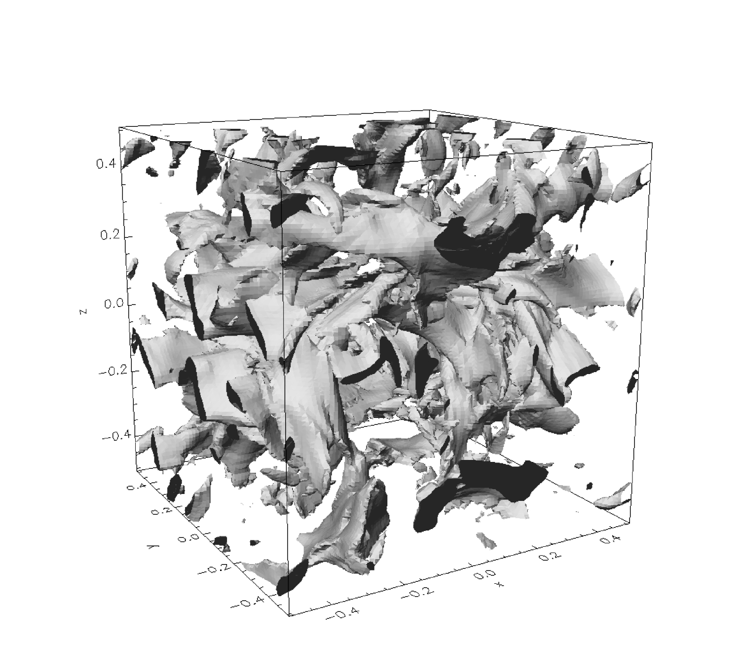
Figure 1: 3D Isosurface plot of the magnetic energy density. The shaded volume surface corresponds to a magnetic energy density of $u_{\mathrm{magn}}\approx 2.5\times 10^{-11}\mathrm{erg}/\mathrm{cm}^{3}$. The spatial extension is given in units of $10^{16}$ cm.

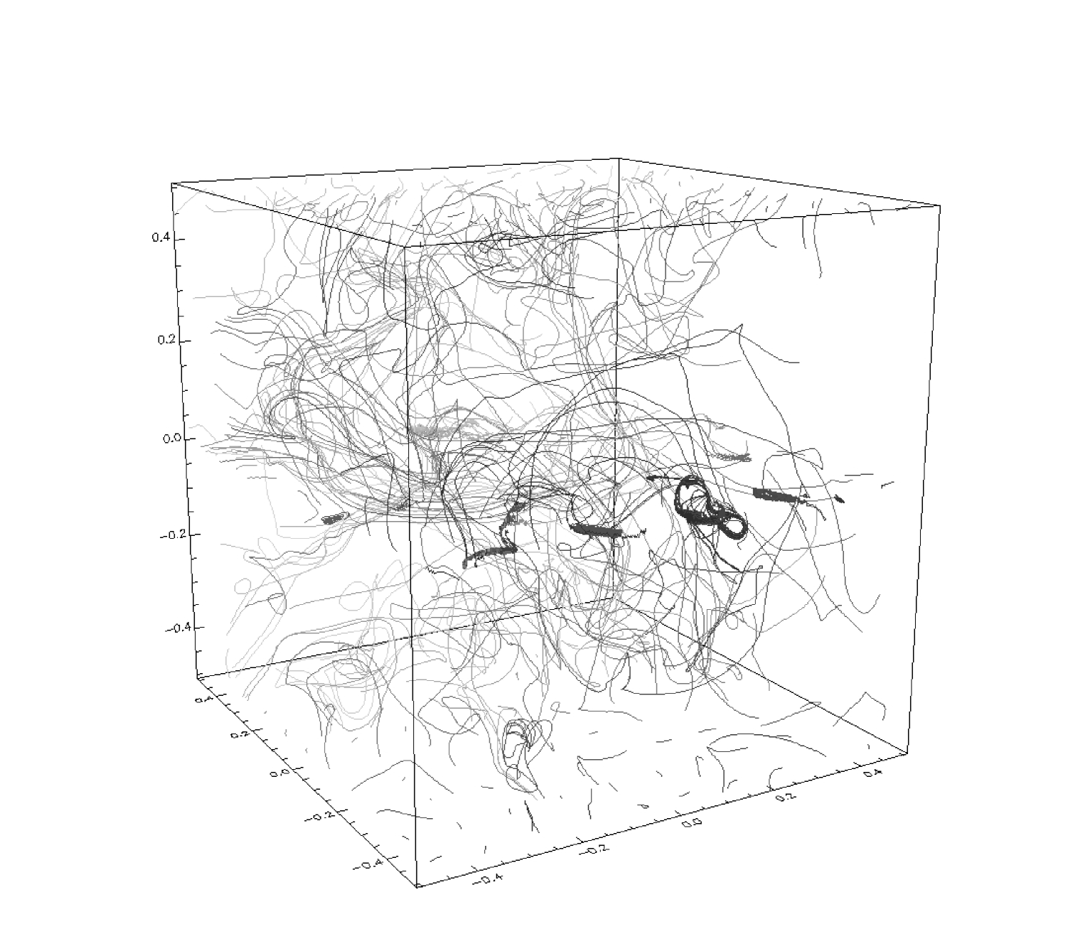
Figure 2: Magnetic field lines.

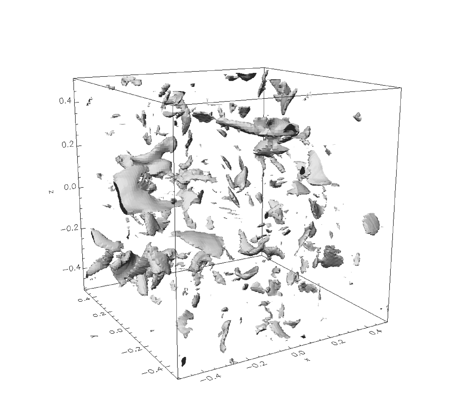
Figure 3: Reconnection regions, i.e. regions with appreciable value of $E_{\|}$. The shaded volume surface corresponds to a value of $E_{\|}\approx 1.3\times 10^{-6},4\times 10^{-7},1.3\times 10^{-7},4\times 10^{-8},1.3\times 10^{-8},4\times 10^{-9}\;\mathrm{statvolt}/\mathrm{cm}$ for the six different test particle runs.

As a result of the resistive MHD calculations we get a turbulent field configuration which we use for the test particle simulations. Fig. 1 and 2 show the magnetic energy density and the magnetic field lines. These figures are to illustrate the turbulent structure of the magnetic field. Fig. 3 shows the reconnection regions, i.e. places where the parallel component of the electric field is appreciable high. These are the acceleration sites where we expect the particles to gain energy. They are also distributed in a very stochastic way clearly indicating the turbulent nature of our fields.

3 Relativistic particle simulations

The MHD calculations described in the previous section are used as the electromagnetic environment for the studies of electron acceleration by means of test particle simulations. We want to know how electric particles behave in the complex three-dimensional turbulent electro-magnetic field configuration, in particular how their energy distribution develops.

The electric field is derived from the MHD quantities $B$, $v$ and $\eta$ by means of the normalized Ohm’s law

$$\mbox{\boldmath$E$}=-\frac{1}{c}\mbox{\boldmath$v$}\times\mbox{\boldmath$B$}+\frac{c}{4\pi}\eta\mbox{\boldmath$\nabla$}\times\mbox{\boldmath$B$},$$ (11)

and gives for the mean value of of the electric field $\overline{E}\approx 0.02\;\overline{B}$. Equation (11) states that a parallel component of the electric field $E_{\|}$ only occurs for $\eta\neq 0$. Compared to the mean perpendicular component $\overline{E}_{\perp}$ the mean parallel component in our simulations is found to be $\overline{E}_{\|}\approx 0.04\;\overline{E}_{\perp}$.

The results of the MHD calculation are scaled to model different physical conditions, i.e. different mass densities inside the nebula, and are then used for the test particle simulations. Here we present the results of particle simulations for six different mean mass densities $\overline{\rho}=10^{n}m_{p}/cm^{3}$, $n=-2,-1,0,1,2,3$ (corresponding to the initial $v_{0}$). The mean magnetic field strength for all runs was chosen to be $\overline{B}=3\times 10^{-4}\;G$.

Since the data for the electric and magnetic field is only available on a discrete three-dimensional grid the test particle code uses linear interpolation to determine the field values for any location. We note that the term ”test particle” means that the electromagnetic fields produced by the particles are not changing the global fields, though the effect of synchrotron radiation on the motion of the particles is taken into account, i.e. the relativistic equations of motion have the form

$$\frac{d\mbox{\boldmath$p$}}{dt}=q\left(\mbox{\boldmath$E$}+\frac{1}{\gamma mc}\,\mbox{\boldmath$p$}\times\mbox{\boldmath$B$}\right)+\mbox{\boldmath$F$}_{Rad}\;,\quad\frac{d\mbox{\boldmath$r$}}{dt}=\frac{\mbox{\boldmath$p$}}{\gamma m},$$ (12)

where $m$ and $q$ denote the mass and charge of the particles, which are electrons in our case and

$$\gamma=\sqrt{1+\left(\frac{p}{mc}\right)^{2}}$$ (13)

is the Lorentz factor.

The calculations are relativistic, including the energy losses via synchrotron radiation and inverse Compton scattering by (Landau & Lifshitz landau (1951))

$$\mbox{\boldmath$F$}_{Rad} \approx \frac{2}{3}\frac{q^{4}}{m^{2}c^{4}}\left\{\mbox{\boldmath$E$}\times\mbox{\boldmath$B$}+\frac{1}{c}\mbox{\boldmath$B$}\times\left(\mbox{\boldmath$B$}\times\mbox{\boldmath$v$}\right)+\frac{1}{c}\mbox{\boldmath$E$}\left(\mbox{\boldmath$E\cdot v$}\right)\right\}$$ (14)

$$- \frac{2}{3}\frac{q^{4}}{m^{2}c^{5}}\gamma^{2}\mbox{\boldmath$v$}\left\{\left(\mbox{\boldmath$E$}+\frac{1}{c}\mbox{\boldmath$v$}\times\mbox{\boldmath$B$}\right)^{2}-\frac{1}{c^{2}}\left(\mbox{\boldmath$E\cdot v$}\right)^{2}\right\}$$

The equations are numerically integrated by a Runge-Kutta algorithm of fourth order with an adaptive stepsize control. As a result we get the momentum and location at certain times of each particle in the given ensemble. The codes has been used before to study high-energy particle acceleration (Nodes et al. nodes (2003); Schopper et al. schopper (1999)).

The direction of the initial momentum vector is equally distributed in a cone of opening angle $80^{\circ}$ at the bottom of the box. This initial condition corresponds to the idea that the electrons enter the the turbulent region moving in a well defined direction. The notion ”final state” relates to a set of particles in which each individual particle has left the computational box.

The simulations start off with electrons injected into the computational box at $z=z_{\rm min}$. We use a powerlaw $E_{kin}^{-2}$ ranging from $10^{2}$ to $10^{4}\;m_{e}c^{2}$ as the initial energy spectrum for all calculations. The choice of this injection spectrum was motivated by our synchrotron model for the infrared to X-ray emission of the Crab pulsar (Crusius-Wätzel, Kunzl & Lesch crusius (2001)). There we could show that the emission of the neutron star could be explained with a single energy distribution $N(E)\propto E_{kin}^{-2}$. We could also show that such an energy distribution is naturalley produced in an efficient pair cascade. Given that plerions in general are powered by a pulsar like in the case of the Crab nebula, an energy distribution $\propto E_{kin}^{-2}$ seems a quite reasonable choice as a probable injection spectrum in turbulent plasmas of a plerionic supernova remnant.

Another series of simulations we performed showed clearly that the resulting energy spectrum is independent of the index of the initial energy distribution. Also the initial energy range does not play a crucial role for the final distribution. After the initial injection of the electrons they get accelerated very rapidly and their energy distribution reaches a stationary state. This happens within only a few days and then the distribution remains for several years until the final state is reached. For different initial distributions only this first acceleration phase gets shorter or longer but the final distribution is given by the energy offered by the MHD fields. Thus, even for a non-relativistic initial energy distribution we expect the final spectral index to be the same as the one found in the relativistic runs.

(a) $\overline{\rho}=0.01\;m_{p}/cm^{3}$

(b) $\overline{\rho}=0.1\;m_{p}/cm^{3}$

(c) $\overline{\rho}=1\;m_{p}/cm^{3}$

(d) $\overline{\rho}=10\;m_{p}/cm^{3}$

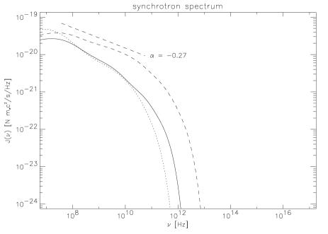
(e) $\overline{\rho}=100\;m_{p}/cm^{3}$

(f) $\overline{\rho}=1000\;m_{p}/cm^{3}$

Figure 4: The initial (dotted line) and final (solid line) energy spectrum of the test particle simulations for different values of the mass density ($\overline{\rho}=10^{n}m_{p}/cm^{3}$, $n=-2,-1,0,1,2,3$). A least squares fit of the spectrum in a certain energy range is plotted above the spectrum and is labeled with the spectral index $s$.

Fig. 4 shows the initial and the final energy spectra of the test particle runs for different values of the mean mass density $\overline{\rho}$. The calculations show that for all values of $\overline{\rho}$ the spectrum gets flatter than the initial spectrum which means that particles are accelerated. Compared to the initial spectrum the low energetic electrons get redistributed to higher energies, i.e. the low energy peak of the initial spectrum is reduced.

The cut-off energy in the spectrum is correlated with the maximum energy that the electrons can gain from the mean parallel component of the electric field $E_{kin}^{max}=el\overline{E}_{\|}$, where $l$ is the length of the computational box.

The final energy spectra can be approximated by a broken power law consisting of two parts: a low energy part which has a relatively flat gradient and a steeper high energy part. Basically the latter part of the spectrum is responsible for the synchrotron radiation therefore we will only consider this part.

For the first run, the one with the lowest density $\overline{\rho}$ we get a spectral index of $-1.19$ for the high energy part above energies of $\gamma\approx 4.0\;10^{3}$. The spectral index $s$ decreases with increasing $\overline{\rho}$ (approximately by a logarithmic relation), i.e. the spectrum gets steeper for denser regions. This result corresponds well with the observed steepening of the radio spectrum at places of magnetic filaments.

(a) $\overline{\rho}=0.01\;m_{p}/cm^{3}$

(b) $\overline{\rho}=0.1\;m_{p}/cm^{3}$

(c) $\overline{\rho}=1\;m_{p}/cm^{3}$

(d) $\overline{\rho}=10\;m_{p}/cm^{3}$

(e) $\overline{\rho}=100\;m_{p}/cm^{3}$

(f) $\overline{\rho}=1000\;m_{p}/cm^{3}$

Figure 5: The initial (dotted line) and the final (solid line) synchrotron spectrum of all runs calculated as the sum of the individual synchrotron spectra of the corresponding electrons (equation (15)). The dashed line depicts the final synchrotron spectrum of a electron population with isotropic pitch angle distribution. The power per unit frequency $J(\nu)$ is normalized to the total rest mass energy $Nmc^{2}$ of the set of electrons, where $N$ is the number of all electrons.

The resulting synchrotron spectrum can be calculated as the sum of total power per frequency emitted by each individual electron. The latter is given by Rybicki & Lightman rybicki (1979)

$$J\left(\frac{\nu}{\nu_{c}}\right)=\frac{\sqrt{3}e^{3}}{mc^{2}}B\sin\theta\frac{\nu}{\nu_{c}}\int_{\nu/\nu_{c}}^{\infty}K_{5/3}(\xi)d\xi,$$ (15)

where $\nu_{c}=\frac{3}{4\pi}\frac{e}{mc}B\gamma^{2}\sin\theta$ is the critical frequency, $\theta$ is the pitch angle and $K_{\frac{5}{3}}$ is the modified Bessel function of order $5/3$. Fig. 5 shows the synchrotron spectra of the high energy particles calculated for the ”real” pitch angle distribution taken from our simulation and a isotropic pitch angle distribution. The isotropic distribution leads to a synchrotron spectrum with spectral index $\alpha=(s-1)/2$ where $s$ is the index of the energy spectrum. This means that the steepening of the energy spectrum with increasing density results in a steepening of the synchrotron spectrum.

The actual final pitch angle distributions in our simulations are clearly anisotropic. In the low density runs the pitch angle distributions offer a peak at $\sin\theta\approx 0.01$. Since $J(\nu)\sim\sin\theta$ the total radiation power emitted is lower as compared to the isotropic case (fig. 5). The pitch angle is also correlated with the gained energy, i.e. the highest energetic particles have the lowest pitch angles. This correlation results from the acceleration along the magnetic field lines for which the parallel component of the electric field $E_{\|}=\left(\eta\mbox{\boldmath$\nabla$}\times\mbox{\boldmath$B$}\right)_{\|}$ is responsible. $E_{\|}$ can only be found at places with significant value of $\eta$. Contrary to second-order acceleration processes the acceleration due to magnetic reconnection is able to explain the observed spectra by particle acceleration in turbulence. To prove the efficiency of acceleration in presence of parallel eletric fields we performed a test particle run without any $E_{\|}$.

Figure 6: Particle energy and synchrotron spectra of a single run with $E_{\|}=0$. The value for the mean density in this run is the same as in the first run in Fig. 4 and Fig. 5 ($\overline{\rho}=10^{-2}m_{p}/cm^{3}$). Due to the lower mean electric field energy the achieved energy levels are lower.

Fig. 6 shows the results of a run that is similar to the first run in Fig. 4 and Fig. 5 with the modification $E_{\|}=0$. The resulting spectra are considerably steeper, since the acceleration is less efficient as in the case with reconnection. Therefore the presence of parallel electric fields is crucial to explain the observed flat spectra. This result is also corroborated by particle simulations starting from an analytic Kraichnan type ideal MHD turbulence (these results will be published elsewhere).

4 Conclusions

We studied the acceleration of relativistic electron populations in three-dimensional reconnective turbulence with applications to the Crab nebula. By means of test particle simulations performed within non-linearly evolved electromagnetic fields modeled by resistive MHD simulations and including radiative losses via synchrotron emission we could show that particles are accelerated and form a energy distribution with powerlaw index $\alpha$ ranging from $1.2$ to $1.6$. We can give limits for the maximum size of the turbulent regions in the nebulae. If the volume is too large and the particle escape time is too long their spectra get significantly harder, i.e. the spectral index is flatter than $1$ (see Fig. 7). For the case of the Crab nebula we can rule out turbulent cells larger than $10^{16}\rm cm$. This limit is in accordance with experimental results from turbulent fluids, in which the turbulence size is limited by the spatial scale of the turbulence source. Since the Crab nebula is powered by a pulsar wind which is shocked at about $10^{17}\rm cm$ the spatial scale of the turbulence should be smaller.

Figure 7: The initial (dotted line) and final (solid line) energy spectrum of a test particle run with larger box size of $l=10^{17}\mathrm{cm}$. The density for this run was chosen to be $\hat{\rho}=10^{-2}m_{p}/cm^{3}$.

We like to suppose the following scenario for the radio emission of the Crab nebula: The nebula is permanently powered by the plasma wind originating from the pulsar. Consequently strong MHD Turbulence is exited in the nebula. In the turbulent regions the leptons experience in situ acceleration in the reconnective turbulent environment. Our simulations prove that the resulting energy spectra and synchrotron spectra are considerably flat and therefore can explain the observed hard radio spectra (Weiler & Shaver weiler2 (1978)). Whereas we concentrate on the Crab nebula, our findings should also be applicable to flat radio spectra of plerions in general. We note, that the efficency of the acceleration within th test particle approach depends on the ratio of Alfven speed to velocity of light which determines the effective electric field strength responsible for particle energization. If the Alfven speed decreases since the magnetic field decreases the electric field will also be weaker, reducing the acceleration to higher energies. If a supernova remnant consists of region with significantly varying magnetic fields and densities the nonthermal particles may be a superposition of particles experiencing different efficencies and electromagnetic fields.

We note that Atoyan (atoyan (1999)) considered the origin of radio emitting electrons in the Crab nebula in terms of intensive radiative and adiabatic cooling in the past. Whereas he argued that effective in situ acceleration in the nebula is not necessary to explain the radio spectra, our simulations prove the capability of magnetic reconnection to energize an electron population of a magnetized plasma under the influence of external electromagnetic fields onto which the accelerated leptons have no back reaction.

References

- (1) Arons, J., 1998, MmSAI 69, 989
- (2) Atoyan, A.M., 1999, A&A 346, L49
- (3) Bandiera, R., 2002, MmSAI 73, 107
- (4) Bandiera, R., Neri, R., Cesaroni, R., 2002, A&A 386, 1044
- (5) Bietenholz, M.F., Kronberg, P.P., 1992, ApJ 393, 206
- (6) Crusius-Wätzel, A., Kunzl, T., Lesch, H., 2001, ApJ 546, 401
- (7) Galant, Y.A., Arons, J., 1994, ApJ 435, 230
- (8) Green, D.A., 1991, PASP 103, 209
- (9) Green, D.A., Scheuer, P.A.G., 1992, MNRAS 258, 833
- (10) Hussein, A.K.M.F., 1983, Phys. Fluids, 26, 2813
- (11) Hussein, A.K.M.F., 1986, J. Fluid Mech. 173, 303
- (12) Kennel, C.F., Coroniti, F.V., 1984a, ApJ 283, 694
- (13) Kennel, C.F., Coroniti, F.V., 1984b, ApJ 283, 710
- (14) Kronberg, P.P., Lesch, H., Ortiz, P.F., Bietenholz, M.F., 1993, ApJ 416, 251
- (15) Landau, L. D., Lifshitz, E. M. 1951, The Classical Theory of Fields (Addison-Wesley, Reading MA.)
- (16) Nodes, C., Birk, G.T., Lesch, H. & Schopper, R. 2003, Phys. Plasmas, 10, 835
- (17) Otto, A., 1990, Comput. Phys. Comm., 59, 185
- (18) Orszag, S. A., Tang, C.-M., 1979, J. Fluid Mechanics, 90, 129
- (19) Rybicki, G. B., Lightman, A. P., Radiative Processes in Astrophysics (Wiley, New York, 1979) ch. 6.2.
- (20) Salvati, M., Bandiera, R., Pacini, F., Woltjer, L., 1998, MmSAI 69, 1023
- (21) Schopper, R., Birk, G.T. & Lesch, H. 1999, Phys. Plasmas, 6, 4318
- (22) Vasyliunas, V.M., 1975, Geophys. Space Phys., 13, 303
- (23) Weiler, K.W., Panagia, N., 1978, A&A 70, 419,
- (24) Weiler, K.W., Shaver, P.A., 1978, A&A 70, 389
- (25) Woltjer, L., Salvati, M., Pacini, F., Bandiera, R., 1997, A&A 325, 295