Stellar polytropes and Navarro–Frenk–White dark matter halos: a connection to Tsallis entropy.

Abstract

We present an alternative for the description of galactic halos based on Tsallis’ non–extensive entropy formalism; on this scheme, halos are stellar polytropes characterized by three parameters, the central density, $\rho_{c}$, the central velocity dispersion, $\sigma_{c}$ and the polytropic index, $n$. To evaluate these parameters we take the Navarro-Frenk-White paradigm as a comparative model and make the following assumptions: both halo models must have the same virial mass, the same total energy and the same maximal velocity. These three conditions fix all the parameters for a given stellar polytrope allowing us to compare both halo models. The halos studied have virial masses on the range $10^{12}-10^{15}\,M_{\odot}$, and it was found after the analysis that they are described, at all scales, by almost the same polytropic index, $n\approx 4.8$, implying an empirical estimation of Tsallis non–extensive parameter for this type of dynamical systems: $q\approx 1.3$.

I Introduction

Cold Dark Matter (CDM) models based on N–body numerical simulations predict excessive substructure and cuspy dark matter halo profiles that are not observed in the rotation curves of dwarf and LSB galaxies Blok1 . The significance of this discrepancy with observations is still under dispute, leading to various theoretical alternatives, either within the thermal paradigm (self–interacting self and/or “warm” warm DM, made of lighter particles), or non–thermal dark matter (DM) models (real DMCQG or complex Ruffini scalar fields, axions, etc). However, none of these alternatives is free of controversy. On the other hand, the CDM model of collision–less WIMP’s could remains still as a viable model to account for DM in galactic halos, provided there is a mechanism to explain the discrepancies of this model with observations in the center of galaxies. The main goal of this paper is to give an approach for such a possibility. The main idea for this alternative is as follows. Since gravity is a long–range interaction and virialized self–gravitating systems are characterized by non–extensive forms of entropy and energy, it is reasonable to expect that the final configurations of halo structure predicted by N–body simulations must be, somehow, related with states of relaxation associated with non–extensive formulations of Statistical Mechanics.

The usual statistical mechanic treatment of self–gravitational systems is provided by the micro-canonical ensemble, which is compatible with negative heat capacities associated with known effects, such as gravothermal instability Padma2 ; Padma3 . An alternative formalism that allows non-extensive forms for entropy and energy has been developed by Tsallis (Tsallis, ) and applied to self–gravitating systems (PL, ; TS1, ; TS2, ), under the assumption of a kinetic theory treatment and a mean field approximation. As opposed to the Maxwell–Boltzmann distribution that follows as the equilibrium state associated with the usual Boltzmann–Gibbs entropy functional, the Tsallis functional yields as equilibrium state the “stellar polytrope”, characterized by a polytropic index $n$. The stellar polytrope yields a Maxwell–Boltzmann distribution function (the isothermal sphere) in the limit $n\to\infty$. This index is related to the “non–extensivity” parameter $q$ of Tsallis entropy functional, so that the “extensivity” limit $q\to 1$ corresponds to the isothermal sphere.

Although the self–gravitating collision-less and virialized gas that makes up galactic halos is far from the state of gravothermal catastrophe, it is reasonable to assume that it is near some form of relaxation equilibrium characterized by non–extensive forms of entropy and energy. On the other hand, high precision N–body numerical simulations, perhaps the most powerful method available for understanding gravitational clustering, roughly yield density, mass and rotation velocity profiles that seem to fit observed galactic halo structures (pending the controversy on excess substructure and cuspy density cores specially on LSB galaxies). Admitting that stellar polytropes follow from an idealized approach based on kinetic theory and an isotropic distribution function, it is still interesting to verify empirically if the structural parameters of the halo gas, or at least of the outcome of numerical simulations, can be adjusted to those of a stellar polytrope, the equilibrium state under Tsallis’ formalism.

It is important to notice that the main objective of this paper is not to compare this polytropic model of dark halo with observational results coming from actual galaxies but with the Navarro-Frenk-White paradigm of dark halos NFW which adequately describes the rotation curves of most galaxies. It is known that the NFW profile fits well the density profile of galaxies in the region outside their core. It fails in the central regions where observations show that the density profile is almost flat. In this work we show that, for example, the best polytropic fit to halos with NFW profiles follows from polytropes characterized by densities in the range $3.7\times 10^{-4}\,\text{M}_{\odot}/\text{pc}^{3}\,<\rho_{c}\,<\,1.2\times 10^{-3}\,\text{M}_{\odot}/\text{pc}^{3}$ and polytropic indices is almost constant with a value near $n=4.8$, or $q\approx 1.3$

Since these best–fit polytropes have the same observable quantities as the NFW halos without central density cusps, they might provide an even better fit to halo structures than the usual NFW profiles. Furthermore, the present analysis and results can be used to calibrate the values of the free parameter $q$ that emerges from Tsallis’s formalism.

Hence, we propose to verify which parameters of the stellar polytropes provide a suitable description of the halo that resembles the one that emerges from the well known numerical simulations of Navarro–Frenk–White. For the wide virial mass range of $10^{10}<M_{\textrm{\tiny{vir}}}/M_{\odot}<10^{15}$.

The paper is organized as follows: in section II we provide the equilibrium equations of stellar polytropes and briefly summarize their connection to Tsallis’ non–extensive entropy formalism. In section III we discuss the dynamical variables of NFW halos, while in section IV we describe a procedure to compare a polytropic halo with an NFW one and obtain numerically the parameters that characterize such polytropic halos, producing graphics showing such comparison. A summary of our results is given in section V.

II Tsallis entropy and stellar polytropes.

For a face space given by $({\bf{r}},\,{\bf{p}})$, the kinetic theory entropy functional associated with Tsallis’ formalism is PL ; TS1 , and TS2

$$S_{q}\ =\ -\frac{1}{q-1}\,\int{(f^{q}-f)\,{d}^{3}{\bf{r}}\,{d}^{3}{\bf{p}}},$$ (1)

where $f$ is the distribution function and $q>1$ is a real number. In the limit $q\rightarrow 1$, the functional (1) leads to the usual Boltzmann–Gibbs functional. The condition $\delta\,S_{q}=0$ leads to the distribution function that corresponds to a stellar polytrope characterized by the equation of state

$$p\ =\ K_{n}\,\rho^{1+1/n},$$ (2)

where $K_{n}$ is a function of the polytropic index $n$, and can be expressed in terms of the central parameters:

$$K_{n}=\frac{{\sigma_{c}}^{2}}{{\rho_{c}}^{1/n}}.$$ (3)

The polytropic index, $n$, is related to the Tsallis’ parameter $q>1$ by:

$$n\ =\ \frac{3}{2}+\frac{1}{q-1}$$ (4)

The stability condition $\delta^{2}S_{q}<0$ is only satisfied generically for polytropes with $3/2<n<5$ (or $9/7<q$), which are then stable equilibrium configurations. Polytropes with $n>5$ are then meta–stable configuration which undergo gravothermal instability for sufficiently large density contrast $\rho/\rho_{c}$ (see TS1 ; TS2 ).

The standard approach for studying spherically symmetric hydrostatic equilibrium in stellar polytropes follows from inserting (2) into Poisson’s equation, leading to the well known Lane–Emden equation B-T

$$\frac{1}{x^{2}}\,\frac{{d}}{{d}x}\left(x^{2}\,\frac{{d}\,\theta}{{d}x}\right)+\theta^{n}\ =\ 0,$$ (5)

with

$$\theta\ = \ \left(\frac{\rho}{\rho_{c}}\right)^{1/n}$$ (6)

$$x\ = \ \frac{r}{r_{0}},\quad r_{0}^{-2}\ =\ \frac{4\pi G\,\rho_{c}}{\sigma_{c}^{2}},\quad\sigma_{c}^{2}\ =\ \frac{p_{c}}{\rho_{c}},$$ (7)

$$G\ =\ 4.297\times 10^{-6}\,\frac{\left(\rm{km/sec}\right)^{2}}{\rm{M}_{\odot}/\rm{kpc}}$$ (8)

where $\sigma_{c}$ and $\rho_{c}$ are the central velocity dispersion and central mass density respectivelly; and we take this value for the gravitational constant due to the units we are using. Notice that the velocity dispersion is a measure of the kinetic temperature of the gas by the relation: $\sigma_{c}^{2}=k_{{}_{B}}\,T_{c}/m$, with $k_{{}_{B}}$ being Boltzmann’s constant, and that we are using a normalization for $r_{0}$, which differs from the usual one by a factor $1/(n+1)$. We find it more convenient to consider instead of (5) the following set of equivalent equilibrium equations

$$\frac{\textrm{d}{\cal{M}}}{\textrm{d}x} =\ x^{2}\,{\cal{Z}},$$

$$\frac{\textrm{d}{\cal{Z}}}{\textrm{d}x} =\ -\frac{n}{n+1}\,\frac{{\cal{M}}\,{\cal{Z}}^{1-1/n}}{x^{2}},$$ (9)

where ${\cal{M}}$ and ${\cal{Z}}$ relate to $M,\,\rho$ (mass and mass density at radius $r$) by

$${\cal{M}} =\ \frac{M}{4\pi\rho_{c}\,r_{0}^{3}},\qquad{\cal{Z}}\ =\ \frac{\rho}{\rho_{c}},$$ (10)

Notice that in the limit $n\to\infty$, equations (9) become the equilibrium equations of the isothermal sphere.

Once the system (9) has been integrated numerically, the velocity profile derived from the virial theorem takes the form:

$$V^{2}(x)\ =\ \sigma_{c}^{2}\,\frac{{\cal{M}}}{x},$$ (11)

where $\sigma_{c}$ can be given in km/sec. The radial distance $r$ in kpc and enclosed mass $M(r)$ in solar masses are given (from (10)) in terms of $x$ and ${\cal{M}}$ by

$$r/{\rm{kpc}} =\ 0.004220\,\,\frac{\sigma_{c}}{\rm{km/sec}}\,\,\left(\frac{\rm{M}_{\odot}/\rm{pc}^{3}}{\rho_{c}}\right)^{1/2}\,\,x,$$ (12)

$$M/{\rm{M}_{\odot}} =\ 944.9737\,\,\left(\frac{\sigma_{c}}{\rm{km/sec}}\right)^{3}\,\,\left(\frac{\rm{M}_{\odot}/\rm{pc^{3}}}{\rho_{c}}\right)^{1/2}\,\,{\cal{M}},$$

Another important dynamical quantity is the total energy of the stellar polytrope TS1 :

$$E\ = \ K+U$$

$$= \ \frac{3}{2}{\int_{0}}^{r}\,4\pi r^{2}P(r)\,dr-{\int_{0}}^{r}{dr\frac{GM(r)}{r}\frac{dM(r)}{dr}},$$

leading to

$$E_{poly}=-\,\frac{1}{n-5}\Big{[}\frac{3}{2}\,\frac{G\,M^{2}}{r}-\Big{(}\frac{\rho}{\rho_{c}}\Big{)}^{1/n}\,\sigma_{c}\Big{(}\frac{3}{2}(n+1)M_{v}-(n-2)4\,\pi\,{r}^{3}\,\rho_{v}\Big{)}\Big{]}$$ (14)

which must be evaluated at a fixed, but arbitrary, value of $r$ marking a cut–off scale.

III NFW halos

NFW numerical simulations yield the following expression for the density profile of virialized galactic halo structures NFW ; Mo , LoMa :

$$\rho_{{}_{\mathrm{NFW}}}=\frac{\delta_{0}\,\rho_{0}}{y\,\left(1+y\right)^{2}},$$ (15)

where:

$$\delta_{0} =\frac{\Delta\,c_{0}^{3}}{3\left[\ln\,(1+c_{0})-c_{0}/(1+c_{0})\right]},$$ (16)

$$\rho_{0} =\rho_{\mathrm{crit}}\,\Omega_{0}\,h^{2}=253.8\,h^{2}\,\Omega_{0}\,\frac{M_{\odot}}{\rm{kpc}^{3}},$$ (17)

$$y =c_{0}\frac{r}{r_{v}},$$ (18)

where $\Omega_{0}$ is the ratio of the total density to the critical density of the Universe, being one for a flat Universe. Notice that we are using a scale parameter ($y$) that is different from that of the stellar polytropes ($x$). The NFW virial radius, $r_{\textrm{\tiny{vir}}}$, is given in terms of the virial mass, $M_{\textrm{\tiny{vir}}}$, by the condition that average halo density equals $\Delta$ times the cosmological density $\rho_{0}$:

$$\Delta\,\rho_{0}=\frac{3\,M_{\textrm{\tiny{vir}}}}{4\,\pi\,r_{\textrm{\tiny{vir}}}^{3}},$$ (19)

where $\Delta$ is a model–dependent numerical factor (for a $\Lambda$CDM model we have $\Delta\sim 100$ at $z=0$ (LoHo, )). It is important to remark that this last relation between the mass and virial radius in terms of cosmological parameters, Eq.(19), is valid for any halo model. The concentration parameter $c_{0}$ can be expressed in terms of $M_{\textrm{\tiny{vir}}}$ by (JZ, ; c0, ):

$$c_{0}\approx 62.1\times\left(\frac{M_{\textrm{\tiny{vir}}}\,h}{M_{\odot}}\right)^{-0.06}$$ (20)

hence all quantities depend on a single free parameter $M_{\textrm{\tiny{vir}}}$. The mass function and circular velocity follow from (15) by $M(r)=4\pi\int{\rho\,r^{2}\,dr}$ and $V^{2}(r)=4\pi\,G\,M/r$, leading to:

$$M=4\,\pi\,\left(\frac{r_{v}}{c_{0}}\right)^{3}\,\delta_{0}\,\rho_{0}\,\left[\ln(1+y)-\frac{y}{1+y}\right],$$ (21)

$$V^{2}=4\,\pi\,G\,\delta_{0}\,\rho_{0}\,\left(\frac{r_{v}}{c_{0}}\right)^{2}\,\left[\frac{\ln(1+y)}{y}-\frac{1}{1+y}\right],$$ (22)

Given $\rho$ and $M$, the gravitational potential per unit mass and radial and tangential pressures follow from:

$$\Phi\,^{\prime} = G\,\frac{M}{r^{2}},$$ (23)

$$P_{r}\,^{\prime} = -\rho\,\Phi\,^{\prime}-\frac{2(P_{r}-P_{\perp})}{r},$$ (24)

which combine to give:

$$P_{r}\,^{\prime}=-G\,\frac{M\,\rho}{r^{2}}-\frac{2\alpha(r)}{r}\,P_{r},$$ (25)

where:

$$\alpha=\frac{P_{r}-P_{\perp}}{P_{r}},$$ (26)

is the anisotropy parameter $0\leq|\alpha|\leq 1$, so that $\alpha=0$ corresponds to an isotropic velocity distribution, since pressure is proportional to velocity dispersion. The parameter $\alpha$ is often taken as a constant in the range $0<\alpha<0.2$, or given by the more realistic empirical ansatz of Ostipov and Merritt LoMa ; OM ; Merr .

The total energy for the NFW halo follows from the general expression (LABEL:eq:E), where $P$ should be obtained from the integration of (25) for a specific form of $\alpha$. As shown by LoMa ; MNS , the curves of $P=\rho\,\sigma^{2}$ obtained from the Ostipov–Merritt ansatz are very close to those of the isotropic case ($\alpha=0$), hence we will consider only isotropic NFW halos. Although analytic solutions of (25) exist for $\alpha=0$ (see LoMa ; MNS ), we will use instead the evaluation of (LABEL:eq:E) obtained by (Mo, ) in which the leading term of the total energy is given by:

$$E_{\rm{\small{NFW}}}=-\,G\,\frac{{M_{\textrm{\tiny{vir}}}}^{2}}{2r_{\textrm{\tiny{vir}}}}\,F_{0}$$ (27)

where $F_{0}$ has the approximate values:

$$F_{0}=\frac{2}{3}+\left(\frac{c_{0}}{21.5}\right)^{0.7}$$ (28)

and $c_{0}$ is given in terms of the virial mass by (20).

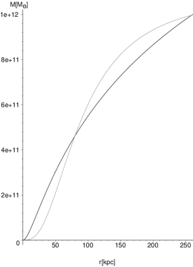
Figure 1: Mass profiles for a NFW halo with $M_{\textrm{\tiny{vir}}}=10^{12}\,M_{\odot}$ and $r_{\textrm{\tiny{vir}}}=260$ kpc (solid curve) and compared fit stellar polytrope (dashed curve).

IV Polytropic and NFW halos comparison.

In order to compare stellar polytropes to NFW halos, it is important to make various physically motivated assumptions. First, we want both models to describe a halo of the same size, but since the virial radius, $r_{\textrm{\tiny{vir}}}$, is the natural “cut–off” length scale at which the halo can be treated as an isolated object in equilibrium, “same size” must mean same virial mass, $M_{\textrm{\tiny{vir}}}$, by equation (19).

Secondly, both models must have the same maximal value for the rotation velocity obtained from (11) and (22). This is a plausible assumption, as it is based on the Tully–Fisher relation, TF , a very well established result that has been tested successfully for galactic systems, showing a strong correlation between the total luminosity of a galaxy and its maximal rotation velocity. It can be shown that the Tully–Fisher relation has a cosmological origin, (JZ, ), associated with the primordial power spectrum of fluctuations (the so called “cosmological Tully-Fisher relation”), hence it is possible to translate the correlation between maximal rotation velocity and total luminosity to a correlation between maximal rotation velocity and total (i.e. virial) mass. Since, by construction we are assuming the polytropic and NFW halos to have the same $M_{\textrm{\tiny{vir}}}$, their maximal rotation velocity must also coincide.

Our third assumption is that the polytropic and NFW halos, complying with the previous requirements, also have the same total energy computed from (27) and from (14) evaluated at the cut–off scale $r=r_{\textrm{\tiny{vir}}}$. The main justification for this assumption follows from the fact that the total energy is a fixed quantity in the collapse and subsequent virialized equilibrium of dark matter halos Padma1 .

Since all structural variables of the NFW halo depend only on the virial mass, once we provide a specific value for $M_{\textrm{\tiny{vir}}}$ all variables become determined in terms of physical units by means of the scale equation (18). Polytropic halos, on the other hand, lack a closed analytic expression for mass, velocity and density profiles. In this case, equations (9) (or (5)) yield numerical solutions for these profiles expressed in terms of the three free parameters $\left\{\rho_{c},\,\sigma_{c},\,n\right\}$. The comparison of these profiles with those of the NFW halos requires that we find explicit values of these free parameters, so that the conditions that we have outlined are met. Since we have selected three comparison criteria for three parameters, we have a mathematically consistent problem. The first constraint on $\left\{\rho_{c},\,\sigma_{c},\,n\right\}$ follows by demanding that, for a given $M_{\textrm{\tiny{vir}}}$ characterizing a NFW halo, we have $M(r_{\textrm{\tiny{vir}}})=M_{\textrm{\tiny{vir}}}$ for the polytropic halo obtained from the numerical solution of (9) with $M$ and $r$ given by (12). A second constraint on the polytropic parameters follows from equating $E_{\rm{poly}}$ from (14), evaluated at $r=r_{\textrm{\tiny{vir}}}$ and $M=M_{\textrm{\tiny{vir}}}$, with $E_{\rm{NFW}}$ from (27). Having fixed two of the polytropic parameters, the third one can be fixed by demanding same maximal velocities in the curves for (11) and (22).

Table 1: Parameters characterizing the polytropes while being compared to NFW halos

$\log_{10}(M_{\textrm{\tiny{vir}}}/M_{\odot})$	$\rho_{c}\,[M_{\odot}/\rm{pc}^{3}]$	$\sigma_{c}\,[\rm{Km/s}]$	$n$	$q$	$K_{n}$	$v_{\rm{max}}\,[\rm{Km/s}]$	$r_{\textrm{\tiny{vir}}}\,[\rm{kpc}]$
15	$3.7\times 10^{-4}$	$982$	$4.93$	$1.29$	$4873.4$	$1504$	$2606.2$
12	$7.5\times 10^{-4}$	$108$	$4.87$	$1.30$	$478.94$	$164$	$260.6$
11	$9.0\times 10^{-4}$	$52$	$4.83$	$1.30$	$221.82$	$79.1$	$120.9$
10	$1.2\times 10^{-3}$	$25$	$4.82$	$1.30$	$100.68$	$38.2$	$56.1$

Following the guidelines described above, we proceed to compare NFW and polytropic halos for $M_{\textrm{\tiny{vir}}}$ ranging from $10^{10}$ up to $10^{15}$ solar masses. From the present comparison we find that the values for central density, $\rho_{c}$, of the polytropic halos are inversely proportional to $M_{\textrm{\tiny{vir}}}$, while the values for the central velocity dispersion, $\sigma_{c}$, are directly proportional to it (this is expected, since $\sigma_{c}$ is a scale parameter in self–gravitating systems). The polytropic index, $n$, is almost constant for the selected range of $M_{\textrm{\tiny{vir}}}$, showing a very small growth as $M_{\textrm{\tiny{vir}}}$ increases. This implies the same qualitative behavior of the Tsallis parameter $q$: it is also almost constant and is slowly increasing as the virial mass grows. It is worthwhile mentioning that the proportionally term $K_{n}$ in the polytropic equation of state (3) shows a very noticeable change, rapidly growing as $M_{\textrm{\tiny{vir}}}$ increases. All these results are displayed explicitly in table 1. The figures depict the mass profiles, figure 1, the velocity profiles, figure 2, and the density profiles, figure 3, for the resulting polytropes with $M_{\textrm{\tiny{vir}}}=10^{12}\,M_{\odot}$, juxtaposed with the same profiles for a NFW halo with same $M_{\textrm{\tiny{vir}}}$. For other values of $M_{\textrm{\tiny{vir}}}$ the mass, velocity and density profiles are qualitatively similar to the ones displayed in these figures.

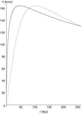
Figure 2: Velocity profiles for the same NFW halo of figure 1 (solid line) and its compared stellar polytrope (dashed curve).

V Conclusions

Motivated by the fact that stellar polytropes are the equilibrium state in Tsallis’ non–extensive entropy formalism, we have found the structural parameters of those stellar polytropes that allows us to compare them with NFW halos of virial masses in the range $10^{10}<M_{\textrm{\tiny{vir}}}/M_{\odot}<10^{15}$. The criteria for this comparison consists in demanding that the polytropes describe a halo having the same virial mass, virial radius, maximal rotation velocity and total energy as the NFW halo. These three conditions are sufficient to determine the three structural parameters $\left\{\rho_{c},\,\sigma_{c},\,n\right\}$ of the polytropic model; the results are displayed in Table 1.

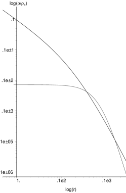
Figure 3: Density profiles for the same NFW halo of figures 1 and 2 (solid curve) and its compared stellar polytrope (dashed curve).

It is important to emphasize that the criteria that determine these polytropes are based on physically motivated assumptions: the virial radius and mass are the natural parameters characterizing the size of a given halo, same maximal velocity follows from the Tully–Fisher relation, while same total energy follows from the virilization process. As shown in Figure 1, the mass distribution of the polytrope grows much slower than that of the NFW halo up to a large radius (100 kpc) containing the core and the region where visible matter concentrates. Hence, as shown by Figure 2, the velocity profile of the polytrope is much less steep in the same region than that of the NFW halo. These features are consistent with the fact that NFW profiles predict more dark matter mass concentration than what is actually observed in a large sample of galaxies (vera, ; LSB, ; JZ, ). Also, as shown in Figure 3, the obtained polytropes have flat cores, very similar to the flat isothermal cores observed in LSB galaxies (as a contrast, the cuspy cores of NFW halos seem to be at odds with these observations (cdm_problems_1, ; cdm_problems_2, ; cdm_problems_3, ), also (vera, ; LSB, )). This flat density core is a nice property, which combined with reasonable mass and velocity profiles, qualifies these polytropes as reasonable (albeit idealized) models of halo structures.

However, in spite of their nice theoretical properties (i.e. their connection to Tsallis’ formalism) and reasonable similarity with equivalent NFW halos, the stellar polytropes we have examined are very idealized configurations and so we are not claiming that they provide a realistic description of halo structures. Instead, we suggest that their described features and their connection with Tsallis’ formalism might indicate that the latter could yield useful information in understanding the evolution and virialization process of dark matter. Although it is necessary to pursue this idea by means of more sophisticated methods, including the use of numerical simulations along the lines pioneered by (TS2, ), the simple approach we have presented has already given interesting results. For example, with respect to the parameter, $q$, we recall that it is a free parameter of the Tsallis’ non-extensive thermodynamics and which has not been fixed for the cosmological case. In this work, by using such statistic in cosmological systems, we are able to determine its behavior as a function of the virial mass, and turns out to be almost constant, with a values around $q\approx 1.2$. This result could be used in other contexts where the extended statistic is also applied Tsallis (2001).

It is well known (B-T, ) that stellar polytropes with $n<5$ (like King halos) have a finite cut–off scale and finite total mass, though for the polytropes that we have studied this cut–off scale is much larger than $r_{\textrm{\tiny{vir}}}$ (just as the “tidal radius” of King halos is much larger than their virial radius). However, as shown in (TS1, ; TS2, ), polytropes characterized by this polytropic index correspond to stable equilibrium states that are generically free from undergoing gravothermal instability.

As mentioned, the results presented in the present work show that a dark matter halo made out of matter which satisfies a polytropic like equation of state, describes the halo in a way as good as the description obtained from the NFW numerical simmulations, that is their paradigm. Furthermore, our description is even nicer as long as it does not have great density growths near the center. However, these results does not directly imply that the dark matter halo do obey a non-extensive entropy formalism. Further tests and expriments are needed in order to consider that such formalism is the one describing the thermodynamics of actual dark matter halos. At the moment, this idea is a possibility which is reinforced by our analysis. We believe these properties to be very encouraging and are currently engaged in a more detailed examination of these polytropes (sigue, ).

- (1) de Blok, W. J. G., MacGaugh, S. S., Bosma, A., and Rubin, V. C., 2001, ApJ, 552, L23; de Blok, W. J. G., MacGaugh, S. S., and Rubin, V. C., 2001, ApJ, 122, 2396; Binney, J. J., and Evans, N. W., 2001, MNRAS, 327, L27; Blais-Ouellette, Carignan, C., and Amram, P., 2002, E-print astro-ph/0203146; Borriello, A. and Salucci, P. MNRAS, 323, 285; Borriello, Salucci, Danese 2002, MNRAS 341, 1109; P. and Burkert, A. 2000, ApJ, 537, L9; P. 2001, MNRAS, 320, L1; P., Walter, F., and Borriello, A., 2002 E-print astro-ph/0206304.
- (2) Spergel, D. N., Steinhardt, P. J., 2000, Phys. Rev. Lett., 84, 3760, E-Print: astro-ph/9909386
- (3) Colin, P., Avila-Reese, V., and Valenzuela, O., 2001,ApJ, 542, 622, E-print: astro-ph/0004115
- (4) Guzmán, F. S., and Matos, T., 2000, Class. Quantum Grav. 17, L9; Guzmán, F. S., and Ureña-López, L. A., 2003, Phys. Rev. D, 68, 024023; Matos, T., and Guzmán, F. S., 2000, Ann. Phys. (Leipzig), 9, SI-133; Matos, T., Guzmán, F. S., and Núñez, D., 2000, Phys. Rev. D, 62, 061301; Matos, T., and Guzmán, F. S., 2001, Class. Quantum Grav., 18, 5055; Matos, T., and Ureña-López, L. A., Class. Quantum Grav., 2000, 17, L75; Matos, T., and Ureña-López, L. A., 2001, Phys. Rev. D, 63, 63506; Matos, T., and Ureña-López, L. A., 2002, Phys. Lett. B 538, 246; Guzmán, F. S., and Ureña-López, L. A., 2004, Phys. Rev. D, 69, 124033; Guzmán, F. S., 2004, Phys. Rev. D, 69, in press;
- (5) Ruffini, R., and Bonazzola S., 1969, Phys. Rev. D, 187, 1767;
- (6) Padmanabhan, T. 1990, Phys. Rep. 188, 285
- (7) Padmanabhan, T. 2000, Theoretical Astrophysics, Volume I: Astrophysical Processes, ed. Cambridge University Press
- (8) Tsallis, C. 1999, Braz J Phys, 29, 1
- (9) Plastino, A. R., & and A Plastino, A. 1993, Phys Lett A, 174, 384
- (10) Taruya, A., & Sakagami, M. 2002, Physica, A 307, 185, e-Print:cond-mat/0107494;
- (11) –, 2003a, Phys. Rev. Lett., 90, 181101; See also –, 2003, e-Print:cond-mat/0310082
- (12) Binney, J., & S. Tremaine, S. 1987, Galactic dynamics, ed. Princeton Univ.
- (13) Navarro, J. F., & Frenk, C. S., & White, S. D. M. 1997, ApJ, 490, 493, e-Print:astro-ph/9611107
- (14) Mo, H. J., & Mao, S., & White, S. D. M. 1998, MNRAS, 295, 319, e-Print:astro-ph/9707093.
- (15) Lokas, E. L., & Mamon, G. 2001, MNRAS, 321, 155
- (16) Lokas, E. L., & Hoffman, Y. 2001, e-Print:astro-ph/0108283. See also Lokas, E. L. 2001, Acta Phys.Polon., B32, 3643
- (17) Avila–Reese, V., et al, 2003, A&A, 412, 633, e-Print:astro-ph/0305516.
- (18) Eke, V. R., & Navarro, J. F., & and Steinmetz, M. 2001, Ap J, 554, 114
- (19) Ostipov, L. P. 1979, PAZh, 5, 77
- (20) Merritt, D. 1985, ApJ, 90, 1027
- (21) Matos, T., & Núñez, D.,& Sussman, R. A. 2004, Gen. Rel. Grav., in press, e-Print:astro-ph/0402157
- (22) Tully, R. B., & Fisher, J. R. 1977, A&A, 54, 661
- (23) Padmanabhan, T. 1993, Structure formation in the universe, Cambridge University Press
- (24) Rubin, V. C., & de Blok, W. J. G., 2001, ApJ, 122, 2381
- (25) Binney, J. J., & Evans, N. W. 2001, MNRAS, 327, L27
- (26) Moore, B. 1994, Nature, 370, 629
- (27) Flores, R., & Primack, J. P. 1994, ApJ, 427, L1
- (28) Burkert, A. 1997, Aspects of Dark Matter in Astro-and Particle Physics (ed. H.V. Klapdor-Kleingrothaus, H. V., & Ramachers, Y.), e-Print: astro-ph/9703057.
- Tsallis (2001) – 2001, ( Eds. Abe, S., & Okamoto, Y. Nonextensive Statistical Mechanics and its Applications, Springer, Berlin, 2001)
- (30) Cabral-Rosetti, L. G., et. al., in preparation.