Prospects for the Detection of Earth-Mass Planets

Abstract

We compare potential state-of-the-art experiments for detecting Earth-mass planets around main-sequence stars using radial velocities, transits, astrometry, and microlensing. For conventionally-discussed signal-to-noise ratio (${\rm S/N}$) thresholds, ${\rm S/N}\sim 8$, the last three methods are roughly comparable in terms of both the total number of planets detected and the mass distribution of their host stars. However we argue that ${\rm S/N}\sim 25$ is a more conservative and realistic ${\rm S/N}$ threshold. We show analytically and numerically that the decline in the number of detections as a function of ${\rm S/N}$ is very steep for radial velocities, transits, and astrometry, such that the number of expected detections at ${\rm S/N}\sim 25$ is more than an order-of-magnitude smaller than at conventional ${\rm S/N}$ thresholds. Indeed, unless Earth-mass planets are very common or are packed much closer to their parent stars than in the solar system, future searches using these methods (as they are currently planned) may not yield any reliable Earth-mass planet detections. On the other hand, microlensing has a much shallower ${\rm S/N}$ slope than the other techniques and so has much greater sensitivity at realistic ${\rm S/N}$ thresholds. We show that even if all stars have Earth-mass planets at periods of one year (and adopting other optimistic assumptions as well), the combined yield of all four techniques would be the detection of only about five such planets at ${\rm S/N}\sim 25$.

1. Introduction

The detection of terrestrial planets around main-sequence stars represents a long-standing major goal of observational astronomy that may finally be realized within the next decade. Terrestrial (i.e. rocky) planets are interesting for several reasons. The frequency, mass, and orbital distribution of planets with masses of $\sim 1-10$ Earth masses ($M_{\oplus}$) yield strong constraints on the physical mechanisms at work in planetary formation and would provide a crucial observational test of planet formation theories. When combined with similar distributions of the properties of more massive planets, this information would allow for stringent tests of core-accretion models for the formation of gas and ice-giant planets (e.g. Ida & Lin 2004). Terrestrial planets are also commonly assumed to be the most favorable places to look for extrasolar life. Especially favored are planets with separations from their parent star that place them in the so-called “habitable zone,” roughly the range of distances at which liquid water can exist, although it is important to keep in mind that not all low-mass planets in the habitable zone are necessarily terrestrial (Kuchner, 2003; Raymond et al., 2004), nor should gas-giant planets in the habitable zone be disregarded, as their satellites may well be capable of supporting life (Williams et al., 1997).

An accurate and robust determination of $\eta_{\oplus}$, the frequency of Earth-mass planets around main-sequence stars, is also essential for the design of future missions that aim to directly image and take spectra of terrestrial planets around the nearest stars, such as the Terrestrial Planet Finder and Darwin. In many design concepts for these missions, the required diameter $D$ of the primary collecting mirror is directly proportional to the distance $d$ of the stars to be surveyed (Beichman, 2004). Thus for a fixed number of planets in the survey volume, $D\propto\eta_{\oplus}^{-1/3}$. Since the cost and feasibility of such missions is likely to be an extremely strong function of $D$, accurate determination of $\eta_{\oplus}$ is essential (Beichman, 2003).

Several different indirect detection techniques have the potential to determine the frequency of terrestrial planets around solar-type stars. Transiting terrestrial planets are detectable photometrically via the periodic dimming of their parent star. For a planet with the radius of the Earth orbiting a main-sequence star, the fractional change in brightness during the transit is $O(10^{-4})$; achieving photometric precisions at this level or better generally requires observations from space (but see Gould et al. 2003b). Also, the low transit probability and duty cycle requires that many stars must be monitored continuously. The space mission Kepler will continuously monitor $\sim 10^{5}$ stars for four years in order to search for transiting planets and will be sensitive to terrestrial planets orbiting in the habitable zones of disk main-sequence stars at distances of $d\sim 1~{}{\rm kpc}$. Terrestrial planets can also be detected from the astrometric wobble they induce on their parent star. For planets of mass $\sim M_{\oplus}$ orbiting at a few ${\rm AU}$ from parent stars located at distances of a few parsecs, the induced displacement is $O({\mu\rm as})$. The Space Interferometry Mission (SIM) will use ultra-high precision astrometry to search for planets in the solar neighborhood ($d\lesssim 20~{}{\rm pc}$), and will be sensitive to planets of a few Earth-masses with orbits of a few ${\rm AU}$ around the most nearby stars (Sozzetti et al., 2002; Ford & Tremaine, 2003; Gould et al., 2003a). Terrestrial planets can be detected via microlensing from the pronounced but brief deviation they induce on microlensing events of their parent stars (Mao & Paczynski, 1991; Gould & Loeb, 1992). Microlensing is potentially very sensitive to Earth-mass planets (Bennett & Rhie, 1996). However, the rarity and brevity of the signal induced by the planets requires the continuous monitoring of a large number of stars. The proposed space mission Microlensing Planet Finder (MPF) (Bennett & Rhie, 2002) would search for planets via microlensing by continuously monitoring $\sim 10^{8}$ main-sequence stars toward the Galactic bulge. This mission would be sensitive to terrestrial planets with few AU orbits around Galactic disk and bulge main-sequence stars at distances of $1-10~{}{\rm kpc}$. Terrestrial planets may also be detectable from the ground with microlensing (Bennett, 2004; Gaudi et al., 2004). Orbiting planets induce radial velocity (RV) variations on their parent stars: an Earth-mass planet orbiting a solar-type star with a period of $0.5~{}{\rm yr}$ induces a RV variation on its parent star of amplitude $\sim 0.1~{}{\rm m~{}s^{-1}}$. This is well below the systematic limit of $1~{}{\rm m~{}s^{-1}}$ typically quoted for current RV surveys. However, it is not clear whether this represents a hard floor, or whether the systematic errors can be averaged out over repeated observations. Therefore, it may also be possible to detect Earth-mass planets from the ground with RV.

Although extrasolar Earth-mass planets have yet to be discovered orbiting main-sequence stars, they have in fact already been discovered around a neutron star using pulsar timing (Wolszczan & Frail, 1992; Wolszczan, 1994; Konacki & Wolszczan, 2003). However, subsequent pulsar searches have shown pulsar planets to be a very rare phenomenon. Furthermore, such planets probably formed after the creation of the pulsar (Hansen, 2002) and are unlikely to be suitable for life.

All of the proposed detection methods discussed above are difficult and require ambitious, cutting-edge experiments. They are therefore both quite expensive and complicated, and thus they require very careful and conservative justification that is based not only on their proposed scientific return, but also on their feasibility and probability of success. To date, discussion has therefore focused on two key issues. First, what information will be learned about such planets if they are detected? Second, how many planets can be detected down to a given threshold in signal-to-noise ratio ${\rm S/N}$? However, there is a third dimension to this discussion that has mostly been ignored: what is the expected distribution of ${\rm S/N}$ with which planets are detected?

At first sight, this appears to be a rather arcane question. In fact, it is crucial. We will argue that, in sharp contrast to experiments that can easily be repeated or that return null results, difficult-to-repeat astronomical experiments that purport to detect novel phenomena must have a high ${\rm S/N}$ threshold to be believable. Or, what amounts effectively to the same thing, a substantial fraction of the detections must be at high ${\rm S/N}$, thereby allowing one to characterize the believability of the detections at lower ${\rm S/N}$. This rule of thumb is unconsciously followed by all observers, or at least all observers who develop respectable track records over the long term. It should also be applied to the daunting task of characterizing Earth-mass planets.

Here we quantify the sensitivity of future experiments to Earth-mass planets using the four proposed techniques: transits, astrometry, RV, and microlensing. We begin by discussing the complementarity of these four techniques, both in terms of the physical parameters measured and the orbital separations of the planets (§2). We then state the methods and assumptions used in evaluating the sensitivity of these techniques (§3). We next discuss the expected form of the ${\rm S/N}$ distribution for each of the four techniques (§4). We present a number of arguments suggesting that conventional ${\rm S/N}$ thresholds are inadequate, and as a result that the number of reliable detections is likely to be considerably smaller than currently envisioned (§5). We then explore the number of expected planet detections from each technique (§6) as a function of the signal-to-noise threshold (§6.1), the primary mass (§6.2), planet period (§6.3), and planet mass (§6.4). We conclude with a discussion of the implications of our results (§7).

2. Complementarity of Proposed Techniques

Different search techniques are intrinsically sensitive to terrestrial planets with different characteristics. In terms of orbital separation, astrometric sensitivity scales as the planet semi-major axis, $a$, while for RV, the sensitivity is $\propto a^{-1/2}$. The sensitivity of a magnitude-limited transit survey is $\propto a^{-5/2}$, but this technique is particularly prized for its ability to detect terrestrial planets in the habitable zone. Microlensing is most sensitive to planets near the Einstein ring of the primary star, which for typical lensing geometries lies at about $a\sim 2.5\,{\rm AU}$. These methods are also complementary in the sense that they measure different physical properties of the planets. Transits provide planet radii, while astrometric measurements provide planet masses. Radial velocity measurements yield the mass of the planet modulo the sine of the inclination of the planetary orbit. In its primitive incarnation, microlensing routinely measures only the mass ratio between the planet and star, although for ambitious next-generation surveys, the mass of the planet will be measurable for a large fraction of the detections (Bennett & Rhie, 2002; Gould et al., 2003; Han et al., 2004). Each method also has other unique advantages. For example, only astrometry and RV routinely probe the architecture of multiple-planet systems, whereas only microlensing can detect Earth-mass planets at very large radii, or free-floating Earth-mass planets that have been ejected from their systems (Bennett & Rhie, 2002; Han et al., 2004).

These differences in sensitivity are basically a good thing: they imply that a coordinated attack on this difficult problem from several directions can substantially increase the range of planet parameters and properties probed. However, while beneficial to science, these differences make it difficult to directly compare the overall sensitivity of different techniques to the detection of terrestrial planets. Fortunately, the main result of this paper, a comparison of the relative distribution functions of ${\rm S/N}$, is generally unaffected by exactly how the comparison is carried out. Rather, this affects only the normalizations of these distribution functions.

3. Methods and Assumptions

In this section we provide our methods and assumptions used in calculating the number of terrestrial planets detectable by each of the four techniques considered. To compute the number of detectable planets, we must specify both the frequency and properties of the planets, as well as the the experimental parameters for each technique.

For most of the results presented in this paper, we consider only planets of mass $M=M_{\oplus}$ (or radius $R=R_{\oplus}$). This is because all the currently known terrestrial planets have $M\leq M_{\oplus}$. However, current theories of planet formation predict that terrestrial planets may have masses of up to $\sim 10~{}M_{\oplus}$, and we therefore consider the sensitivity of the techniques as a function of planet mass in §6.4. In order to be as democratic as possible, we begin by assuming orbital periods that allow each method to play to its strengths. For astrometry, RV, and microlensing, we assume that the planets are all located at periods at which the detection sensitivity of the particular method is maximized (or nearly so). For transits, we assume the planets are located in the habitable zones of their parent stars. Our specific choices are somewhat arbitrary, and in §6.3 we explore the sensitivity of the various methods as a function of orbital period. Finally, we assume that every main-sequence star surveyed has a planet of the specified parameters.

We specify the experimental parameters for each technique that are appropriate to either planned space missions, or future ground-based surveys of our own conception. Again, our choices here are somewhat arbitrary, and one could consider other choices for the experimental parameters. However, we consider our choices to represent the most ambitious yet feasible experiments of their kind, and therefore to be very optimistic.

Radial Velocity: We assume that each star has a planet with $M=M_{\oplus}$ and period $P=0.5\,\rm yr$. We assume a total observing time and photon collection rate appropriate to four dedicated 2m telescopes over 5 years. This corresponds to 60,000 hours of dedicated observations. We assume a systematics limit of $\sigma=1\,\rm m\,s^{-1}$ and take the error to be $\sigma=(1+10^{0.4[V-1.5]})^{1/2}\,\rm m\,s^{-1}$ for a 2 minute exposure. Note that, in terms total photon collecting power, this is approximately equivalent to 500 hours per year for 5 years on Keck. However, the combination of four dedicated 2m telescopes is much superior to the Keck scenario for stars $V<5$ because the fixed overhead time per target is a much smaller percentage of the exposure time.

Astrometry: We assume that each star has a planet with $M=M_{\oplus}$ and $P=3\,\rm yr$. We assume a survey of 40,000 astrometric measurements each with systematics-limited errors of $\sigma=1\,{\mu\rm as}$. This corresponds to 2,000 hours of SIM time per year over 5 years, with each measurement taking 15 minutes. To account for the photon noise of faint stars, we assume an error $\sigma=(1+10^{0.4[V-11]})^{1/2}{\mu\rm as}$.

Transits: We assume each star has a planet with $R=R_{\oplus}$ located in the habitable zone, defined as $a=(L_{\rm bol}/L_{{\rm bol},\odot})^{1/2}{\rm AU}$, where $L_{\rm bol}/L_{{\rm bol},\odot}$ is the bolometric luminosity of the parent star relative to the Sun. We use the parameters of the Kepler satellite, except that we augment the sample to include faint nearby stars as advocated by Gould et al. (2003b), thereby multiplying the detection rate by a factor 2.5 relative to the original Kepler strategy.

Microlensing: We assume that each main-sequence star has an Earth-mass planet at $a=2.5\,{\rm AU}$. We use the results of a simulation by Gaudi et al. (2004) of a 5-year ground-based microlensing search using four 2m wide-field telescopes located in Chile, South Africa, Australia, and Hawaii. This simulation adopts the star-count based normalization of the optical depth calculated by Han & Gould (2003). The form of the derived S/N distribution is similar to that of the MPF satellite (Bennett & Rhie, 2002), but the normalization is about 30% smaller when the latter is rescaled using the same optical depth derived by Han & Gould (2003).

For transits and microlensing, the above descriptions serve to completely describe the experiment, but for astrometry and RV they do not. Transits and microlensing are carried out in survey mode, so that every star is, by definition, observed in exactly the same way. Astrometry and RV are pointed experiments in which the observer is free to divide up the observing time among targets with more or less complete freedom. In our baseline comparison, we will force astrometry and RV into survey mode. That is, we will demand that they allocate the same amount of observing time to each of their program stars. We determine the number of program stars, $N$, by rank ordering all stars in the Hipparcos catalog (ESA, 1997) according to their sensitivity under each respective method, and then requiring that a $1\,M_{\oplus}$ planet in a favorable orbit (edge-on for RV, face on for astrometry) around the $N$th star can be detected at ${\rm S/N}=5$ by using $1/N$ of the total observing time. This may not be the optimal choice and is certainly not how current RV surveys are carried out. Hence, in § 4.1 we also consider alternative observing scenarios.

Of course, our assumptions are idealized in that they do not take account of both recognized and unrecognized effects. For example, photospheric variations will prevent $\sigma=1\,\rm m\,s^{-1}$ measurements for some RV targets; some reference stars required to fix the local reference frame of astrometric targets will be found to be astrometrically unstable; some transit targets will be too variable for reliable photometric monitoring; we ignore binary stars completely. Since problems of this type are likely to affect all methods, and their actual magnitude cannot be estimated with high precision in advance, we ignore them here. As nearly all unaccounted-for effects will serve to degrade the sensitivities, our assumptions tend to be optimistic.

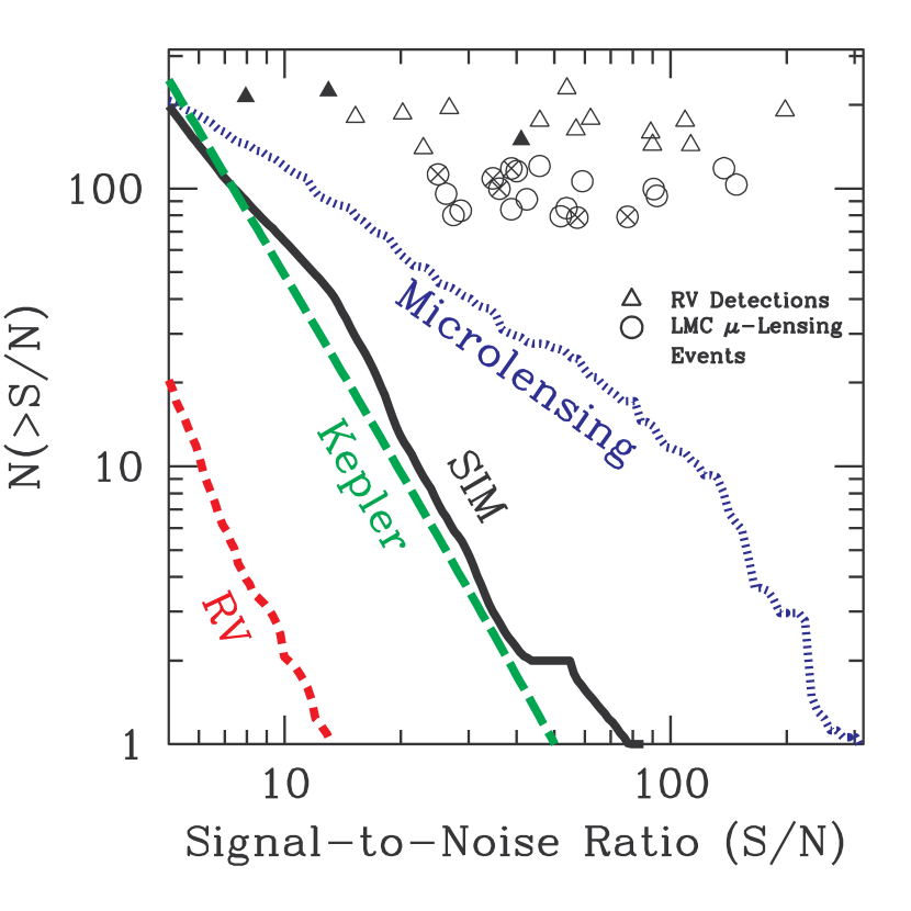
Figure 1.— Number of detectable Earth-mass planets as a function of threshold in S/N. Each experiment is allowed to play to its strengths; it is assumed that all stars have planets with: $P=0.5\,$yr for the RV survey; $P=3\,$yr for astrometry (SIM); $a=2.5\,{\rm AU}$ for microlensing; and $a=(L_{\rm bol}/L_{{\rm bol},\odot})^{1/2}{\rm AU}$ for transits. Symbols show the actual S/N of detections in two challenging historical experiments. Circles passed the basic cuts as microlensing events toward the LMC as reported by Alcock et al. (2000), but circles with crosses were later found to be background SNe, not microlensing events. Triangles are RV detections of planets. Filled triangles are detections that are ambiguous, controversial, or have been retracted.

4. Scaling with Signal-to-Noise Ratio

Figure 1 and Table 1 compare the distribution of signal-to-noise ratios of all four methods. Here we define the signal-to-noise ratio as ${\rm S/N}\equiv(\Delta\chi^{2})^{1/2}$, where $\Delta\chi^{2}$ is the difference in $\chi^{2}$ in the best-fitting models with and without a planet. The scalings with ${\rm S/N}$ are all basically power laws $N\propto({\rm S/N})_{\rm min}^{-\nu}$, except for the case of microlensing, for which the scaling is a broken power law. Why do the functions take this form and why is the slope for microlensing so much shallower than the other methods? While each curve is the result of a complex numerical integration, it is nevertheless possible to basically understand the origins of all four slopes using fairly simple reasoning. In each case, we need to ask, given an ensemble of detections with S/N above some threshold, what subset of these detections will have twice that S/N?

Let us begin with Kepler transits. Consider a star of given spectral type for which a planet can just barely be detected at ${\rm S/N}=({\rm S/N})_{\rm min}$. Where can one find a star of the same spectral type with ${\rm S/N}=2({\rm S/N})_{\rm min}$? Clearly, if another star were closer by a factor 2, it would yield 4 times greater flux and so twice as much S/N. However, there are 8 times fewer of such nearby stars, so $\nu=3$. Why then is the slope in Figure 1 $\nu=2.4$ and not exactly 3? As discussed by Gould et al. (2003b), the Kepler $10^{\prime\prime}$ point spread function (PSF) contains about $V=17$ of sky, which fundamentally limits its sensitivity to otherwise detectable planets around M dwarfs. For each adopted threshold $({\rm S/N})_{\rm min}$, there is some spectral class of stars for which coming closer by a factor 2 moves the star from below the sky to above it, and this implies that it is not quite necessary to reduce the sample size by a factor 8 to double $({\rm S/N})_{\rm min}$. If all stars were above the sky, the slope would be $\nu=3$. If all were below the sky, the slope would be $\nu=1.5$. The actual value of $\nu=2.4$ results from competition between these two regimes.

The reasoning is quite similar for SIM astrometry. In this case, the astrometric precision does not depend on distance for most stars that will be monitored because the systematics limit sets in relatively faint at $V=11$. Since the astrometric signature scales inversely as the distance, while the astrometric noise is distance-independent, the S/N also scales inversely as the distance. So, just as with Kepler, one expects $\nu=3$. However, just as with Kepler, this scaling is broken by a second-order effect. Some stars are $V\gtrsim 11$ and hence are in the photometric not systematics limit. In the photometric limit, one expects $\nu=1.5$. The net value of $\nu=2.4$ again results from competition.

For RV, the situation is qualitatively similar. In the photon limit, one expects $\nu=3$, just as for Kepler. Although very few stars have $V<1.5$ (the regime dominated by systematics), some are this bright. Once systematics set in, there is no improvement in S/N obtained by moving the star closer. Hence, $\nu=\infty$. The net result is that $\nu=3.1$, i.e., slightly higher than the value obtained in the photon limit.

For microlensing, the situation is very different from the other three methods. First, the sources of light are independent of the planets and their hosts, and furthermore, are all at essentially the same distance (i.e., the Galactocentric distance $R_{0}\sim 8~{}{\rm kpc}$). Therefore, the distribution of photometric errors directly reflects the shape of the source-star luminosity function. Second, there is large distribution of signal amplitudes $\delta$ for a given planetary system. Therefore, in order to find a higher ${\rm S/N}$ event, one can either look at a brighter source stars, or “wait” for the rare events that have higher intrinsic signal amplitudes. It is possible to demonstrate numerically that, for a planet with mass ratio $q$ located near the Einstein ring of its primary, the area of the Einstein ring that is photometrically perturbed by the planet by a fractional amount $>\delta$ is $\Omega\propto q\delta^{-1}$. This is in the limit of point sources; in reality this distribution will be cut off at a some maximum deviation $\delta_{\rm max}$ due to finite-source effects. The luminosity function in the Galactic bulge is well-represented by a broken power-law, with ${\rm d}N/{\rm d}{\rm log}{L}\propto L^{-1/3}$ for stars fainter than the turn-off, and $\propto L^{-1.3}$ for stars brighter than the turn-off (Holtzman et al., 1998). Stars fainter than the turn-off are fainter than the combined sky plus unresolved star background, and thus ${\rm S/N}\propto L\Omega^{1/2}\delta\propto Lq^{1/4}\delta^{3/4}$, where the $\Omega^{1/2}$ term arises from the assumption that the typical duration of perturbations is $\propto\Omega^{1/2}$. Stars brighter than the turnoff are typically above the background, and thus ${\rm S/N}\propto L^{1/2}q^{1/4}\delta^{3/4}$. These basic ingredients combine to yield the broken power-law behavior in seen in Figure 1. We note that, for a space-based mission such as MPF, essentially all sources are above the background. Therefore, for sources below the turn-off the scaling with ${\rm S/N}$ is expected to be steeper than for the ground-based scenario (although the overall normalization is higher), as is seen in the results of the simulations of Bennett & Rhie (2002).

TABLE 1
Number of Detectable Planets
Method ${\rm S/N}>5$ ${\rm S/N}>10$ ${\rm S/N}>25$ ${\rm S/N}>50$ ${\rm S/N}>100$ RV (Survey) 22 2 0 0 0 SIM (Survey) 207 65 7 2 0 Microlensing 208 121 46 26 11 Kepler 246 49 6 1 0 ${\rm S/N}=5$ ${\rm S/N}=10$ ${\rm S/N}=25$ ${\rm S/N}=50$ ${\rm S/N}=100$ RV (Optimized) 38 15 5 2 0 SIM (Optimized) 335 174 76 37 17

4.1. Flexibility of Astrometry and RV

Recall that in constructing Figure 1, we handicapped the astrometric and RV experiments to mimic surveys. That is, we required them to expend the same observing time on all targets. The transit and microlensing surveys must do this, but in reality astrometry and RV are not so constrained. We illustrate this flexibility by considering an alternative set of strategies. Here we first choose an arbitrary number $N$ and pick out the $N$ stars with the best sensitivities from our rank-ordered list of Hipparcos stars. We divide all the available observing time among these $N$ stars in such a way that each has equal final S/N. That is, the worst stars from among the list are observed more frequently (or with longer exposures) than the best. The result of this exercise is shown by the chains of filled circles in Figure 2, which should be contrasted with the corresponding curves taken from Figure 1. Table 1 compares the number of detected planets at or above several selected ${\rm S/N}$ under these two different observational strategies. It is important to emphasize that the curves represent one experiment, while the circles represent many different possible experiments, only one of which can be realized. That is, if every star has a planet, and the astrometric observations follow the survey strategy, then there will be three detections with ${\rm S/N}>40$ and 30 detections with ${\rm S/N}>16$. However, if the alternative strategy is used, one has a choice of three detections with ${\rm S/N}=500$ or 30 detections with ${\rm S/N}=60$. One cannot have both.

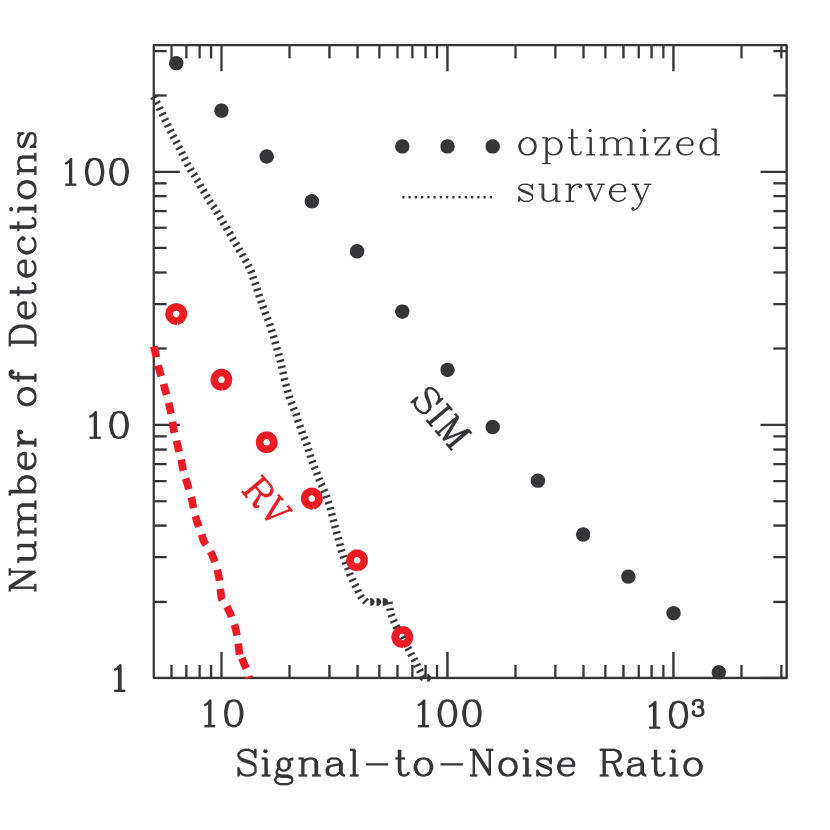
Figure 2.— Flexibility of RV and astrometry (SIM). Curves are the same as Fig. 1 and represent the sensitivity of these techniques if they are forced into “survey mode”, in which each target star is observed for the same total amount of time. Dashed curve is for RV, dotted curve is for SIM. Circles represent a series of different experiments, in each of which the exposure times are tailored to obtain the same S/N for each target star. That is, there are more detections at a fixed S/N but at the price of not having a tail of detections at substantially higher S/N. Filled circles are for SIM, open circles are for RV.

5. Conservative Signal-to-Noise Thresholds

What is the appropriate S/N cutoff? The answer to this question depends on one’s definition of “appropriate.” Traditionally, the appropriate value of the minimum S/N threshold has been set by just considering statistics. One can ask, given the expected properties of the noise and signal, what S/N threshold is necessary in order that less than some tolerated number of false alarms are expected. Determination of this “statistical” $({\rm S/N})_{\rm min}$ can be quite complicated and requires careful consideration of both the expected distribution of measurement noise as well as the number of statistically independent trials needed to thoroughly search the data (see, e.g., Jenkins et al. 2002).

Thresholds set based on statistics alone are the least conservative and the most optimistic, in the sense that it is statistically impossible to detect a signal with any confidence at a lower threshold. While such thresholds maximize the number of detected planets, we argue that they are dangerous and undesirable for several reasons. First, for the majority of the “detections”, which are near this minimum threshold, one has used essentially all of the available information simply to detect the signal. This means that it is generally impossible to determine the nature of the signal, i.e., to measure planetary parameters or to use the detailed form of the signal to corroborate its interpretation. Simply speaking, all one is confident of is that something has been detected – there is essentially no information about exactly what has been detected. As a result, such detections are extremely prone to being confused with false positives. Given that, for many of these experiments, follow-up and independent confirmation of the candidates will be difficult or impossible, this is a serious concern. We discuss this in more detail below. Furthermore, even if false positives can be reliably excluded, it is still the case that the parameters of the detected planets will be very poorly constrained, making the scientific usefulness of the detections questionable.

We argue that the actual S/N threshold adopted should consider both the ability to extract physical parameters from the detected planets, as well as the possible presence of false positives, and the inability to perform follow-up of the detections. The threshold required to measure planetary parameters to a given precision depends on many different quantities, such as the complexity of the signal, the cadence, sampling, and duration of the observations, etc. This issue has been most thoroughly explored in the case of SIM (Sozzetti et al., 2002, 2003; Ford & Tremaine, 2003). Very roughly, these authors find that thresholds of ${\rm S/N}\gtrsim 25$ are required to constrain the planetary parameters to better than $30\%$. For transits, the situation is considerably better, as the period of transiting planets should be measured with exquisite precision even for low ${\rm S/N}$ detections, and the fractional error in the planetary radius is $\sim 0.5({\rm S/N})^{-1}\lesssim 2\%$ for ${\rm S/N}>25$. For microlensing, the simulations of Gaudi et al. (2004) indicate that, for $90\%$ of the perturbations detected with ${\rm S/N}>25$, the planet/star mass ratio should be measurable to $\lesssim 30\%$. No comprehensive study of the ability to extract planet parameters from RV curves has been performed, but it seems likely that, given the nature of the observations, the uncertainties will be similar to those for astrometric data.

What ${\rm S/N}$ threshold is required to deal with false positives? Until the experiments are actually carried out, and false positives are identified, one cannot be certain. However, it is instructive to consider historical precedent. Figure 1 summarizes two relevant experiences. The first is the 5.7-year microlensing dark-matter search toward the Large Magellanic Cloud (LMC) by the MACHO collaboration (Alcock et al., 2000). Like the proposed planet searches, the MACHO experiment was a massive search for objects that are extremely difficult to detect. Because the detections involve events that are over, and hence can never be verified individually, MACHO was compelled to be very conservative in what they called a “detection”. They demanded $({\rm S/N})_{\rm min}=20$. Nevertheless, there is substantial debate in the microlensing community as to whether they were conservative enough. Figure 1 illustrates one reason why. The circles show the S/N of all the events surviving the basic selection cuts. However, circles with crosses were eliminated because they were judged to be probable supernovae (SNe). How they came to be recognized as such is very instructive in the current context. Originally, SNe were not considered as a possible background. It was only because two of the SNe “events” had very high ${\rm S/N}\sim 60$ (see Fig. 1) that their character as SNe was recognizable. Then other, lower S/N, events were examined for telltale SN signatures. If all the events had had ${\rm S/N}<40$, it is unlikely the SNe would have ever been recognized. For this reason, one may also wonder whether some of the other “low-quality” (${\rm S/N}\sim 30$!) events are due to some other unanticipated astrophysical effect. Alcock et al. (2000) were not able to prove that they were not. However, because of the strong tail of very high S/N events, they were able to show that their conclusions did not rest on these events that were open to question: they repeated their analysis, progressively increasing $({\rm S/N})_{\rm min}$, and showed that their conclusions did not change (although of course their statistical errors then deteriorated). The high S/N tail therefore gave credence to lower S/N events, at least statistically, and these then allowed MACHO to better characterize the population they were detecting.

Also shown in Figure 1 is a (non-exhaustive) sample of RV planet detections from Cumming et al. (1999) and Vogt et al. (2002). Note that the great majority of these have very high S/N. This partly reflects the extreme conservatism of the observers. This conservatism is practiced by the majority of the RV observational community and is reflected in the fact that, while the typically quoted single-measurement RV error is only a few ${\rm m~{}s^{-1}}$, very few planets have been announced with velocity semi-amplitude $\lesssim 20~{}{\rm m~{}s^{-1}}$. It is just such conservatism that has established the RV planets as bedrock facts rather than hopeful speculation. The RV detections of planets around HD219542b and $\epsilon$ Eri are the exceptions that prove the rule. The tentative detection of a planet around HD219542b was originally claimed by Desidera et al. (2003). This detection was at ${\rm S/N}\sim 8$, near the ${\rm S/N}$ threshold proposed for terrestrial planet searches. However, Desidera et al. (2003) cautioned that the RV variations could also be due to stellar activity. Indeed, Desidera et al. (2004) recently reported additional measurements indicating that the RV variations are indeed most likely due to stellar activity. The RV detection of a planet around $\epsilon$ Eri was at an even higher ${\rm S/N}\sim 13$ (Hatzes et al., 2000). However, despite this relatively high S/N (by the standards of proposed terrestrial planet searches) and despite the strong external prior favoring a planet around $\epsilon$ Eri (Nimoy, 1975, 1995), this detection remains controversial. Also very instructive is the extremely strong (${\rm S/N}\sim 40$) detection reported for HD192263 (Santos et al., 2000), which was later refuted (Henry et al., 2002) and then subsequently reasserted (Santos et al., 2003). All three of these examples show that extreme caution is warranted when probing for extreme or novel phenomena.

The microlensing-like SNe, HD219542b, and $\epsilon$ Eri demonstrate that it is difficult to break new scientific ground with detections that, while formally robust, lack the S/N to unambiguously characterize the object that has been detected. On the contrary, the significance of such ambiguous “detections” can only be evaluated provided that the sample includes other detections that are completely unambiguous.

Now, it is true that experiments yielding null results can and do operate at or near the pure-noise limit. For example, Gilliland et al. (2000) was able to set limits on planets in 47 Tuc going down to a threshold $({\rm S/N})_{\rm min}=6.3$ at which point they expected $O(1)$ false detection due to Gaussian noise. Gaudi et al. (2002) searched for planetary signatures in 43 microlensing events down to $({\rm S/N})_{\rm min}=7.7$, a factor 1.5 higher than the threshold dictated by Gaussian noise. Their retreat from this threshold is highly instructive. They found about a half dozen events above the Gaussian threshold but below their adopted one. They concluded that these could not be regarded as reliable planet detections partly because a Monte Carlo analysis of stable light curves showed a similar S/N distribution, and partly because of the expected form of the microlensing S/N distribution shown in Figure 1. That is, if a substantial fraction of these marginal “detections” were real, one would also expect other detections at much higher S/N. This again demonstrates that without good sensitivity to high S/N detections, a cutting-edge experiment cannot reliably interpret the marginal detections.

6. Results

6.1. Number of Planets at Realistic Thresholds

Considering all the arguments presented in §5, we conclude that, although thresholds of $({\rm S/N})_{\rm min}\sim 8$ may yield formally statistically significant detections, conservative thresholds of $({\rm S/N})_{\rm min}\sim 25$ should be adopted for the ambitious, cutting-edge experiments discussed here. In light of this conclusion, it is instructive to reconsider the signal-to-noise scalings show in Figure 1 and discussed in §4. Table 1 summarizes the number of expected Earth-mass planet detections for various values of $({\rm S/N})_{\rm min}$. Several important points are worth mentioning. First, although transits (Kepler), astrometry (SIM), and microlensing all have similar sensitivities when compared at a minimal requirement $({\rm S/N})_{\rm min}=8$, the sensitivities of both SIM and Kepler fall off very steeply compared to microlensing ($N\propto({\rm S/N})_{\rm min}^{-2.4}$ versus $N\propto({\rm S/N})_{\rm min}^{-1}$). As a result, at the conservative threshold of $({\rm S/N})_{\rm min}=25$, microlensing is 5 times more sensitive than either transits or astrometry. Furthermore, for the specific assumptions (see §3) adopted here, the total number of Earth-mass planets detected by Kepler and SIM above this threshold is relatively small, $\lesssim 10$. In the case of SIM, this may be improved by more judicious appropriation of the observing time (§4.1), and the situation will be better for shorter periods (for Kepler) or longer periods (for SIM). However, it is generally the case that the assumptions we have made are optimistic, as we have ignored known (and unanticipated) effects that will degrade the sensitivity, assumed that all stars have Earth-mass planets, and assumed observational strategies that are more aggressive than those currently being planned for these experiments. Therefore, it seems likely that, when more realistic assumptions are adopted, the number of expected robust detection of Earth-mass planets will be modest.

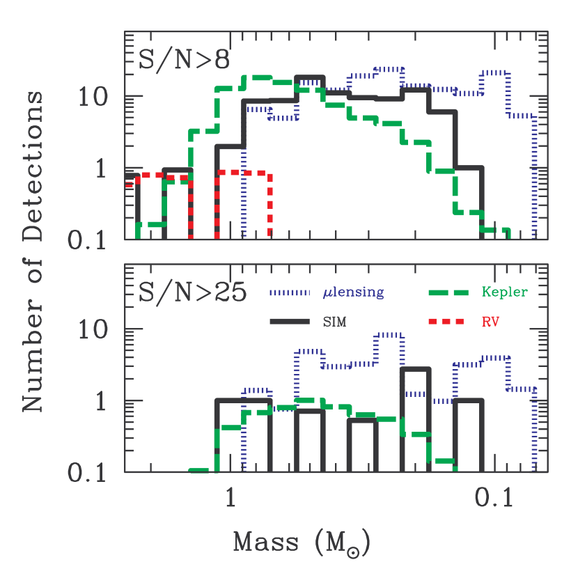
Figure 3.— Distributions of parent-star masses for the experiments summarized in Fig. 1, for two different S/N thresholds, $({\rm S/N})_{\rm min}=8$ and $({\rm S/N})_{\rm min}=25$. At $({\rm S/N})_{\rm min}=8$, microlensing, transits (Kepler), and astrometry (SIM) all have comparably broad parent-star mass distributions with comparable normalizations. At $({\rm S/N})_{\rm min}=25$, the forms of the distributions remain similar, but microlensing has a much higher normalization than the other two.

6.2. Sensitivity as a Function of Stellar Mass

What are the masses of the stars whose planets would be detected in the four surveys summarized in Figure 1? Figure 3 shows these distributions for two different S/N thresholds, $({\rm S/N})_{\rm min}=8$ and $({\rm S/N})_{\rm min}=25$.

At $({\rm S/N})_{\rm min}=8$, which is similar to the thresholds that are customarily discussed in this field, microlensing, astrometry, and transits all have rather similar distributions, with microlensing extending to somewhat lower masses and transits to somewhat higher masses. These broad distributions primarily reflect the breadth of the underlying stellar mass function. The Kepler experiment tends to be cut off at low masses because these faint stars fall below the sky of its $10^{\prime\prime}$ PSF (Gould et al., 2003b). Microlensing is cut off at high masses because there are no such stars in the Galactic bulge, which is the location of most of the lens population. RV is especially sensitive to high-mass stars because these are bright and, except for stars $V\lesssim 1.5$, our assumed sensitivity scales $\propto 10^{-0.2V}$. In fact, the most massive stars in the RV histogram are A stars and therefore probably inaccessible to RV. This subtlety has been ignored in our simple prescription for detectability based on $V$ flux alone.

However, as we discussed in § 5, historical experience argues against the viability and believability of ${\rm S/N}=8$ detections in challenging experiments of this type. Based on this historical experience, we believe that the experimental design should hinge on the expected number and distribution of detections at much higher S/N, perhaps $({\rm S/N})_{\rm min}=25$. This is also shown in Figure 3. The functional forms of the distributions are similar to the case of $({\rm S/N})_{\rm min}=8$, but the amplitudes are reduced. As expected from Figure 1 and the scaling relations discussed in § 4, microlensing drops by about a factor of 3, while astrometry and transits drop by about a factor 15. RV would not detect Earth-mass planets at all at this threshold.

6.3. Sensitivity as a Function of Planet Period

As discussed in § 2, our primary comparison of different techniques has allowed each to play to its strengths. While democratic, this approach also means that Figures 1–3 do not reflect the relative detectability of the same ensemble of planetary systems. To better understand the complementarity of different techniques that was discussed in § 2, we plot in Figure 4 the number of detectable planets as a function of period, $P$. In this case, we assume that each star has one planet at each period. As expected, transits and RV are primarily sensitive to short-period planets, while microlensing and astrometry are primarily sensitive to long-period planets.

6.4. Sensitivity as a Function of Planet Mass

For the majority of the discussion, we have concentrated on planets with $M=M_{\oplus}$ (or $R=R_{\oplus}$), since all the currently-known terrestrial planets have a mass $\lesssim M_{\oplus}$. However, some theories of planet formation predict that considerably more massive terrestrial planets with $M\lesssim 10~{}M_{\oplus}$ may be common (e.g., Kokubo & Ida 2002; Raymond et al. 2004; Ida & Lin 2004). Therefore we briefly consider the number of expected planet detections as a function of the mass of the planet. For both RV and astrometry, the signal is directly proportional to the mass of the planet. When combined with the ${\rm S/N}$ scalings from §4, this yields $N\propto M^{2.4}$ for astrometry and $N\propto M^{3.1}$ for RV. For Kepler, the signal is $\propto R^{2}$, or, assuming constant planet densities, $\propto M^{2/3}$. Therefore, $N\propto M^{1.6}$. Finally, for microlensing, the signal is $\propto M^{1/4}$. However, here we must also consider the increase in the detection probability for the larger mass ratios, which is $\propto M^{1/2}$. This yields, for sources below the turnoff and fainter than the background, $N\propto M^{3/4}$. We confirm this scaling in our simulations.

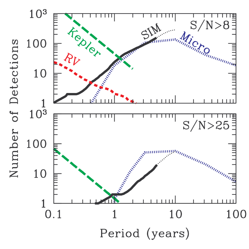
Figure 4.— Sensitivity to planets as a function of period $P$ for the four techniques. In contrast to Figs 1–3, here it is assumed that every star has a planet with period $P$, so that each technique is confronted with the same ensemble of planetary systems. Transits (Kepler) are truncated at $P=2\,$yr because Kepler is a four-year experiment that must detect at least 2 transits. Astrometry (SIM) has a dotted-line extension from $P=5\,$yr to $P=10\,$yr to reflect the possible extension of this mission from 5 to 10 years. The survey designs are identical to those described in § 2, and the indicated S/N thresholds are the same as in Fig. 3.

7. Discussion

As discussed in § 2, and demonstrated in Figures 1 and 4, the four detection techniques reviewed here are very distinct, not only in terms of their sensitivity as a function of ${\rm S/N}$ and period, but also in the information they yield about the planets. In addition, there are number of secondary characteristics of the planet sample gathered by the experiments that are unique to each of the four methods. These characteristics may also be important to consider when assessing how well-suited a given method is to fulfilling a particular task. In the following, we examine the relative strengths and weakness of each method, considering both the primary and secondary characteristics of the planet harvest, and concentrating on five interrelated considerations: the total number of planets detected, the sensitivity to habitable planets, the ability to robustly calibrate the frequency of terrestrial planets as required for the success of TPF, the location and nature of the planet-bearing stars, and the opportunity for follow-up of the detected planets and hosts.

The RV planet search envisioned here is clearly the least competitive in terms of the total number of planets detected. Even an optimized search using 4 dedicated 2m telescopes searching for 5 years would only allow the detection (at ${\rm S/N}=25$) of Earth-mass planets with $P=0.5~{}{\rm yr}$ around the five best candidate host stars. The sensitivity is further reduced for planets in the habitable zone. On the other hand, the technology required to initiate such a search is already available, and the detection of even one such planet would be very interesting, because the host stars would be very nearby $d\lesssim 20~{}{\rm pc}$, and thus promising targets for detailed follow-up with ground-based instruments, as well as TPF. Furthermore, the fact that such a search is ground-based and targeted means that it is very flexible. Therefore, it may be possible to search for Earth-mass planets around a larger number of stars using a two-tier survey approach, in which promising targets from an initial, low-${\rm S/N}$ survey are followed up more intensively to yield high-${\rm S/N}$ detections. Finally, RV searches are advantageous in that they can detect multi-planet systems, with both gas-giant and terrestrial planets, providing essential constraints on the effects of massive planets on terrestrial planet formation. Furthermore, planets detected via RV can be confirmed by SIM, yielding planet masses.

In ‘survey’ mode, in which all targets are allocated the same amount of observing time, and for conservative thresholds of $({\rm S/N})=25$, SIM will detect at most $\sim 10$ Earth-mass planets at $P=3~{}{\rm yr}$. For the largest detectable period corresponding to the nominal mission lifetime of $P=5~{}{\rm yr}$, $\sim 30$ Earth-mass planets are detectable. However, it may be possible to detect as many as $\sim 80$ Earth-mass planets at ${\rm S/N}=25$ and $P=3~{}{\rm yr}$ if the search is optimized, and the observing time is allocated according to the sensitivity of the host star to planets (see §4.1). As discussed above in the context of RV searches, it may be possible to survey an even larger number of stars for Earth-mass planets by adopting a dynamic, two-tier approach. SIM will also be sensitive to planets in the habitable zone of some target stars (Sozzetti et al., 2002), although maximizing the number of detections of such planets requires a modification of the observing strategy (Gould et al., 2003a). In addition, the stars surveyed by SIM are exactly those which can be targeted by TPF, making the results of the SIM planet search critical. However, we emphasize that the results presented here assume a very ambitious SIM planet search. In particular, we have assumed that a total of $\sim 10,000$ hours, or $\sim 20\%$ of the available SIM time, is devoted to searching for planets. Currently only $\sim 8\%$ of SIM time is allocated to searching for planets around nearby main-sequence stars, in two SIM key projects. Furthermore, the two key projects are not currently optimized to find Earth-mass planets. Therefore, achieving the results presented here will require not only an increase in the amount of time alloted to planet searches, but also a careful reassessment of the observing strategies.

The primary advantage of Kepler is that it will be sensitive to Earth-mass planets in the habitable zone. Unfortunately, at conservative thresholds of ${\rm S/N}\sim 25$, Kepler will only find $\sim 6$ Earth-mass habitable planets. Although the detection of even one such planet would be extremely interesting, this is an insufficient number to accurately constrain the frequency of such planets. Therefore, constraints on this frequency will have to be derived from lower ${\rm S/N}$ observations, or from extrapolations from the frequency of higher-mass planets. Both of these procedures are potentially risky. Kepler is much more sensitive to planets with shorter periods (see Figure 4), and should provide robust statistics on terrestrial-mass planets close to their parent stars. Follow-up of candidate Earth-mass planets detected by Kepler will be difficult. The target stars of Kepler are disk main-sequence stars at distances of $\sim{\rm kpc}$, and thus will be too faint ($V>9$) or distant for confirmation with either RV or SIM. Naively, one might expect the Hubble Space Telescope (HST), provided that it is still operational, to yield ${\rm S/N}$ that are larger by a factor of two, given that its aperture is twice that of Kepler. However, this is more than compensated for by the fact that Kepler’s bandpass is larger by a factor of $\sim 10$ than the $50~{}{\rm nm}$ bandpass used to observe the transiting planet HD209458b, which Brown et al. (2001) found to yield photon rates that are a factor of $\sim 5$ smaller than those expected for Kepler for stars of the same magnitude. Therefore, one expects ${\rm S/N}$ that are a factor of $\sim 2$ smaller for HST. It may be possible to follow-up candidate transit events in the infrared using the James Webb Space Telescope (JWST). This will depend on the photometric precision of the available JWST instruments and on whether it is launched in time to confirm the Kepler transits before their phases are lost.

Of the four methods we have discussed, microlensing is the most sensitive in terms of the total number of potential planet detections at realistic ${\rm S/N}$ thresholds. At ${\rm S/N}\sim 25$, a 5-year ground-based microlensing survey of the kind envisioned here could potentially detect $\sim 50$ Earth-mass planets at $a=2.5~{}{\rm AU}$. Therefore, microlensing could constrain the frequency of terrestrial planets to reasonable precision. Although such a survey would also be sensitive to Earth-mass planets at $\sim 1{\rm AU}$, this is only for low-mass target stars, and thus microlensing is not able to directly constrain the frequency of Earth-mass planets in the habitable zone. While a ground-based microlensing survey is attractive in that it is flexible, relatively inexpensive, and does not rely on untested technology, the results stated above are predicated on the ability to achieve near photon-limited photometry on stars with $I\gtrsim 20$ (Gaudi et al., 2004). This may be difficult in the crowded fields toward the Galactic bulge (Bennett, 2004). A space-based microlensing survey such as MPF would circumvent the problems with crowded-field photometry. Detailed simulations of a space-based microlensing survey indicate that it would yield a detection rate of Earth-mass planets at $\sim 2.5{\rm AU}$ that is higher than the ground-based survey by at least $\sim 30\%$ (Bennett & Rhie, 2002). Furthermore, the space-based survey would be sensitive to planets over a wider range of semi-major axes, and would be considerably more sensitive to multiple planets. Both ground- and spaced-based microlensing surveys are sensitive to Earth-mass planets surrounding main-sequence stars with distances of $1-10~{}{\rm kpc}$. It is important to emphasize that microlensing is sensitive to planets around both Galactic bulge and disk stars. For example, in the simulations of Gaudi et al. (2004), $\sim 30\%$ of the detected Earth-mass planets orbit disk main-sequence stars. Because of the large distances to the lens stars, follow-up of detected planet candidates will be difficult. However, in many cases the lens star should be sufficiently bright to be detectable, and it will be possible to constrain the mass of the primary, and thus the mass of the planet (Bennett & Rhie, 2002). Furthermore, by combining ground and space-based surveys, it should be possible to routinely measure planet masses (Gould et al., 2003). However, direct confirmation of the planet candidates via, e.g. RV or astrometric follow-up, will be essentially impossible in the foreseeable future.

The synergy of the four methods for detecting Earth-mass planets is clear from Figure 4, which demonstrates the possibility of searching for Earth-mass planets over many decades in period by combining a variety of techniques. Since nothing whatsoever is known about the distribution or frequency of Earth-mass planets around other stars, no technique can be guaranteed to be the most sensitive. Any technique could yield null results if the regions of its greatest sensitivity were sparsely populated by planets. Therefore, a combined attack on the problem using all four techniques is indicated. The discussions above indicate that the result of such a coordinated search for planets could go a long way toward answering many of the questions of interest, and would provide important calibrations for the next generation of experiments, including direct searches like TPF and Darwin.

That said, the results presented here, and in particular as shown in Figure 4, also reveal some rather sobering realities. The combined sensitivity of the four techniques reaches its nadir at $P\sim 1\,$yr, near the periods of the only two Earth-mass planets known to be orbiting a main-sequence star. Furthermore, at the $({\rm S/N})_{\rm min}=25$ threshold that historical experience suggests is the minimum for reliable results on such cutting-edge experiments, the number of expected detections of Earth-mass planets with $P\sim 1\,{\rm yr}$ is frighteningly low. Even if all stars had such planets and even if all four of these techniques were funded and/or allocated telescope time at the level we have somewhat optimistically supposed, and even if all worked according to their specifications, only about 5 such planets would be detected at $({\rm S/N})_{\rm min}=25$. Indeed, unless Earth-mass planets are very common, or unless they are packed much closer to their parent stars than is true in the solar system, then it is possible that neither Kepler nor SIM (as they are currently planned) would yield any reliable, high-${\rm S/N}$ Earth-mass planet detections.

References

- Alcock et al. (2000) Alcock, C. et al. 2000, ApJ, 542, 281
- Beichman (2003) Beichman, C. A. 2003, ESA SP-539: Earths: DARWIN/TPF and the Search for Extrasolar Terrestrial Planets, 271
- Beichman (2004) Beichman, C. 2004, in ASP Conf. Ser. 000, Planetary Systems in the Universe, eds. A. Penny, P. Artymowicz, A.-M. Lagrange, & S. Russel (ASP: San Francisco), 000
- Bennett (2004) Bennett, D.P. 2004, in the Proceedings of the XIXth IAP Colloquim, Extrasolar Planets Today and Tomorrow (astro-ph/0404075)
- Bennett & Rhie (1996) Bennett, D.P., & Rhie, S.H. 1996, ApJ, 472, 660
- Bennett & Rhie (2002) Bennett, D.P., & Rhie, S.H. 2002, ApJ, 574, 985
- Brown et al. (2001) Brown, T. M., Charbonneau, D., Gilliland, R. L., Noyes, R. W., & Burrows, A. 2001, ApJ, 552, 699
- Butler et al. (2002) Butler, R.P., et al. 2002, ApJ, 578, 565
- Cumming et al. (1999) Cumming, A., Marcy, G. W., & Butler, R. P. 1999, ApJ, 526, 890
- Desidera et al. (2003) Desidera, S., et al. 2003, A&A, 405, 207
- Desidera et al. (2004) Desidera, S., et al. 2004, A&A Letters, in press (astro-ph/0405054)
- ESA (1997) European Space Agency (ESA). 1997, The Hipparcos and Tycho Catalogues (SP-1200; Noordwijk: ESA)
- Ford & Tremaine (2003) Ford, E. B. & Tremaine, S. 2003, PASP, 115, 1171
- Gaudi et al. (2002) Gaudi, B.S., et al. 2002, ApJ566, 463
- Gaudi et al. (2004) Gaudi, B.S., Han, C. & Gould, A. 2004, in preparation
- Gilliland et al. (2000) Gilliland, R.L., et al. 2000, ApJ, 545, L47
- Gould et al. (2003) Gould, A., Gaudi, B. S., & Han, C. 2003, ApJ, 591, L53
- Gould & Loeb (1992) Gould, A. & Loeb, A. 1992, ApJ, 396, 104
- Gould et al. (2003a) Gould, A., Ford, E. B., & Fischer, D. A. 2003a, ApJ, 591, L155
- Gould et al. (2003b) Gould, A., Pepper, J., & DePoy, D. L. 2003b, ApJ, 594, 533
- Han & Gould (2003) Han, C. & Gould, A. 2003, ApJ, 592, 172
- Han et al. (2004) Han, C., Chung, S., Kim, D., Park, B., Ryu, Y., Kang, S., & Lee, D. W. 2004, ApJ, 604, 372
- Hansen (2002) Hansen, B.M.S. 2002, ASP Conf. Proc. 263, Stellar Collisions, Mergers and their Consequences, ASP Conference Proceedings, ed. M. M. Shara (ASP: San Francisco), 221
- Hatzes et al. (2000) Hatzes, A.P., et al. 2000, ApJ, 544, L145
- Henry et al. (2002) Henry, G. W., Donahue, R. A., & Baliunas, S. L. 2002, ApJ, 577, L111
- Holtzman et al. (1998) Holtzman, J. A., Watson, A. M., Baum, W. A., Grillmair, C. J., Groth, E. J., Light, R. M., Lynds, R., & O’Neil, E. J. 1998, AJ, 115, 1946
- Ida & Lin (2004) Ida, S. & Lin, D. N. C. 2004, ApJ, 604, 388
- Jenkins et al. (2002) Jenkins, J. M., Caldwell, D. A., & Borucki, W. J. 2002, ApJ, 564, 495
- Kokubo & Ida (2002) Kokubo, E. & Ida, S. 2002, ApJ, 581, 666
- Konacki & Wolszczan (2003) Konacki, M. & Wolszczan, A. 2003, ApJ, 591, L147
- Kuchner (2003) Kuchner, M. J. 2003, ApJ, 596, L105
- Mao & Paczynski (1991) Mao, S. & Paczynski, B. 1991, ApJ, 374, L37
- Nimoy (1975) Nimoy, L. 1975, I Am Not Spock (Milbrae:Celestial Arts)
- Nimoy (1995) Nimoy, L. 1995, I Am Spock (New York:Hyperion)
- Pepper et al. (2003) Pepper, J., Gould, A., & Depoy, D. L. 2003, Acta Astronomica, 53, 213
- Raymond et al. (2004) Raymond, S. N., Quinn, T., & Lunine, J. I. 2004, Icarus, 168, 1
- Santos et al. (2000) Santos, N. C., Mayor, M., Naef, D., Pepe, F., Queloz, D., Udry, S., Burnet, M., & Revaz, Y. 2000, A&A, 356, 599
- Santos et al. (2003) Santos, N. C., et al. 2003, A&A, 406, 373
- Sozzetti et al. (2002) Sozzetti, A., Casertano, S., Brown, R. A., & Lattanzi, M. G. 2002, PASP, 114, 1173
- Sozzetti et al. (2003) Sozzetti, A., Casertano, S., Brown, R. A., & Lattanzi, M. G. 2003, PASP, 115, 1072
- Vogt et al. (2002) Vogt, S. S., Butler, R. P., Marcy, G. W., Fischer, D. A., Pourbaix, D., Apps, K., & Laughlin, G. 2002, ApJ, 568, 352
- Williams et al. (1997) Williams, D. M., Kasting, J. F., & Wade, R. A. 1997, Nature, 385, 234
- Wolszczan & Frail (1992) Wolszczan, A., & Frail, D. A. 1992, Nature, 355, 145
- Wolszczan (1994) Wolszczan, A. 1994, Science, 264, 538