The Geneva-Copenhagen survey of the Solar neighbourhood

We present and discuss new determinations of metallicity, rotation, age, kinematics, and Galactic orbits for a complete, magnitude-limited, and kinematically unbiased sample of 16,682 nearby F and G dwarf stars. Our $\sim$63,000 new, accurate radial-velocity observations for nearly 13,500 stars allow identification of most of the binary stars in the sample and, together with published $uvby\beta$ photometry, Hipparcos parallaxes, Tycho-2 proper motions, and a few earlier radial velocities, complete the kinematic information for 14,139 stars. These high-quality velocity data are supplemented by effective temperatures and metallicities newly derived from recent and/or revised calibrations. The remaining stars either lack Hipparcos data or have fast rotation.
A major effort has been devoted to the determination of new isochrone ages for all stars for which this is possible. Particular attention has been given to a realistic treatment of statistical biases and error estimates, as standard techniques tend to underestimate these effects and introduce spurious features in the age distributions. Our ages agree well with those by Edvardsson et al. (edv93 (1993)), despite several astrophysical and computational improvements since then. We demonstrate, however, how strong observational and theoretical biases cause the distribution of the observed ages to be very different from that of the true age distribution of the sample.
Among the many basic relations of the Galactic disk that can be reinvestigated from the data presented here, we revisit the metallicity distribution of the G dwarfs and the age-metallicity, age-velocity, and metallicity-velocity relations of the Solar neighbourhood. Our first results confirm the lack of metal-poor G dwarfs relative to closed-box model predictions (the “G dwarf problem”), the existence of radial metallicity gradients in the disk, the small change in mean metallicity of the thin disk since its formation and the substantial scatter in metallicity at all ages, and the continuing kinematic heating of the thin disk with an efficiency consistent with that expected for a combination of spiral arms and giant molecular clouds. Distinct features in the distribution of the $V$ component of the space motion are extended in age and metallicity, corresponding to the effects of stochastic spiral waves rather than classical moving groups, and may complicate the identification of thick-disk stars from kinematic criteria. More advanced analyses of this rich material will require careful simulations of the selection criteria for the sample and the distribution of observational errors.

1 Background and motivation

The Solar neighbourhood is the benchmark test for models of the Galactic disk: The stars in a sample volume around the Sun provide a first estimate of the mass density of the Galactic disk near the plane. Their distribution in age is our record of the star formation history of the disk. Their overall and detailed heavy-element abundances as functions of age are the fossil record of the chemical evolution and enrichment history of the disk. Finally, the space motions and Galactic orbits of the stars as functions of age are our clues to the parallel dynamical evolution of the Galaxy and the degree of mixing of stellar populations from different regions of the disk (see, e.g. the recent review by Freeman & Bland-Hawthorn freeman02 (2002)).

Providing the basic data for the stars of the Solar neighbourhood – ages, metallicities, velocities, and Galactic orbits – may seem the simplest observational task of all. Yet, the identification of the nearest stars and the data needed for a proper characterisation of their main astrophysical parameters remain seriously incomplete. Moreover, stars have often been selected for observation from criteria which induce correlations between the observed parameters that reflect the characteristics of the selection process more strongly than those of the Galaxy. Intrinsic parameters such as the frequency, age, and metallicity of groups of stars are intertwined with such easily observable properties as brightness, colours, and proper motions in ways that can make it difficult or impossible to retrieve the former from the latter. Kinematic selection biases are particularly pernicious in this regard.

F- and G-type dwarf stars are favourite tracer populations of the history of the disk. They are relatively numerous and sufficiently long-lived to survive from the formation of the disk; their convective atmospheres reflect their initial chemical composition; and ages can be estimated for at least the more evolved stars by comparison with stellar evolution models. Photometry in the Strömgren $uvby\beta$ system is an efficient means to derive their intrinsic properties from observation (Strömgren stromgren63 (1963), stromgren87 (1987)). Recent studies based mainly on $uvby\beta$ photometry are, e.g. Feltzing et al. (feltz01 (2001)), Holmberg (holmb01 (2001)), and Jørgensen (bjarner00 (2000)), while more detailed spectroscopic studies of the chemical history of selected subsets of stars have been made by, e.g. Edvardsson et al. (edv93 (1993)), Fuhrmann (fuhrm98 (1998)), Reddy et al. (reddy03 (2003)), and Bensby et al. (bensby03 (2003)).

Extensive $uvby\beta$ photometric surveys of the nearby F and G stars have been performed by Olsen (eho83 (1983, 1993); 1994a ; 1994b ). Accurate parallaxes and proper motions have become available for large numbers of these stars from the Hipparcos (ESA hipp97 (1997)) and Tycho-2 (Høg et al. tycho2 (2000)) catalogues. The bottleneck so far has been the corresponding radial-velocity data. These are needed, first, to complete the three-dimensional space motions for all the stars and improve the statistical accuracy of the derived age-velocity relations. They also serve to identify those stars which just happen to pass near the Sun at present, but were formed elsewhere and have witnessed another evolutionary history than that of the Solar circle. Finally, and perhaps most importantly, repeated radial-velocity measurements allow identification of the large fraction of stars in the photometric samples which are binaries, and for which the derived astrophysical and kinematical data will be inaccurate and potentially misleading.

The key contribution of this paper consists of new, accurate, radial velocities for an all-sky, magnitude-limited and kinematically unbiased sample of $\sim$13,500 nearby F and G stars, based on $\sim$63,000 individual photoelectric observations. Because this data set is unlikely to be superseded in essential respects until the results of the GAIA mission (Perryman et al. gaia01 (2001)) and/or the RAVE project (Steinmetz steinmetz (2003)) become available, we have also recalibrated and redetermined the astrophysical parameters ($T_{eff}$, $M_{v}$, and [Fe/H]) for all stars in our sample. Much effort has been devoted to the fundamental issue of determining reliable isochrone ages for as many stars as possible, and we believe that a rather more realistic assessment of the errors of such ages has been obtained. Finally, we have computed individual Galactic orbits for all stars with adequate data.

Table 1: Table 1 is only available in electronic form at the CDS. The first two pages of the table, listing the first 100 stars, are given at the end of this paper as sample of its content and format.

The resulting data set should place a wide range of studies of the evolution of the Galactic disk on a new and considerably improved footing. We caution, however, that no such thing as a fully unbiased sample exists in Galactic astronomy, and the reader is strongly urged to carefully study Sect. 5, where we discuss the key issue of completeness of the data, especially as regards the derived ages and masses. The catalogue with the complete data set for 16,682 stars will be available electronically (sample pages are shown in Table 2).

The complementarity between the present study and the much-quoted paper by Edvardsson et al. (edv93 (1993)) deserves clarification. The 189 stars studied by Edvardsson et al. (edv93 (1993)) were drawn from the kinematically unbiased sample presented here, selecting equal numbers of stars in 10 metallicity bins through the range of [Fe/H] seen in the (thin and thick) disk. Evolved F dwarfs were selected, excluding known binaries and fast-rotating stars, so that interstellar reddening and isochrone ages could be determined. Thus, unevolved stars were avoided, young metal-poor and old metal-rich stars were excluded a priori by the colour cutoffs used, and the sample was strongly biased in favour of metal-poor stars. The sample discussed here was explicitly designed to alleviate these selection biases and further benefits from the advent of the Hipparcos and Tycho-2 data but, for obvious reasons, lacks the detailed, precise, and homogeneous spectroscopy that was the centrepiece of the study by Edvardsson et al. (edv93 (1993)).

The present paper is organised as follows: Sect. 2 clarifies the selection criteria used to define the sample, and Sect. 3 describes the new radial velocities and other basic observational material available for the stars. Sect. 4 explains the (partly new) calibrations and analysis methods we have used to derive reliable astrophysical parameters from the raw data, and Sect. 5 discusses the completeness and various biases in the resulting parameter sets. We briefly rediscuss some of the classical diagnostic diagrams in Sect. 6 and finally summarise our conclusions and some of the prospects for the future in Sect. 7.

2 Sample definition

From the outset, it was clear that the definitive selection and characterisation of the nearby F and G dwarfs should be made from a comprehensive photometric survey in the Strömgren $uvby\beta$ system. But in order to undertake such a survey, an observing list is needed. Thus, the first step in the project was to establish an apparent-magnitude limited, kinematically unbiased all-sky sample of stars within which the F and G dwarfs would also be volume-complete to a sufficiently large distance ($\sim$40 pc).

For this, we chose the HD catalogue (Cannon & Pickering 1918- (24)), the only all-sky spectral catalogue then available. All A5-G0 stars brighter than $m_{vis}$ = 8.3, G0 stars in the interval 8.30$\leq m_{vis}\leq$8.40, and all G5 or just G stars (no subtypes) brighter than $m_{vis}$ = 8.6 were selected. On the one hand, the A5 spectral-type limit is early enough to include even quite metal-poor F stars; on the other hand, most K0-type stars in the HD catalogue are giant stars for which luminosities, distances, tangential velocities, and ages cannot be reliably determined.

It was desirable to also include any old, metal-rich dwarfs and thus improve the observational basis for a reassessment of the “G-dwarf problem”. However, observing the vast numbers of HD K-type giants is an inefficient way to identify such stars. We therefore added all 1,277 G0V-K2V stars south of $\delta$ = -26$\degr$ from the Michigan Spectral Catalogues (Houk & Cowley 1975, Houk 1978, 1982) that were previously unobserved, but estimated from the spectral types and $m_{pg}$ to be within a distance of 50 pc, with generous allowance for the uncertainties. This sample should be complete to about the same distance limit (40 pc) as the rest of the G-dwarf sample, but covers only part (28%) of the entire sky.

The vast majority of all these stars ($\sim$30,000 in total) were then observed in the $uvby\beta$ photometric surveys described below, and the sample for the radial-velocity programme was defined from the measured photometric indices. Subsequently, the Hipparcos and Tycho-2 catalogues have provided accurate parallaxes and proper motions for nearly all the stars for which radial velocities had been measured.

2.1 Initial photometric survey

From the observing lists assembled as described above, nearly all stars were observed at least once in the Strömgren $uvby\beta$ system by Olsen (eho83 (1983, 1993); 1994a ; 1994b ). The resulting catalogues were merged with previous sources of $uvby\beta$ photometry (Strömgren & Perry stromper65 (1965); Crawford et al. crawbar66 (1966, 1970); 1971a ; 1971b ; crawbar72 (1972, 1973); Grønbech & Olsen gronbech76 (1976, 1977), and Olsen & Perry ehoper84 (1984)). The combined FG photometric catalogue thus constructed contains a total of 30,465 stars.

This all-sky sample is complete to the magnitude limits described above and should be volume complete for the F and G dwarfs to a distance of $\sim$40 pc. In the southern cap where modern MK spectral types are available, the G0V-K2V stars within the same distance are also included. This homogeneous, complete, and kinematically unbiased database was used to select stars for the radial-velocity programme, using the criteria described below.

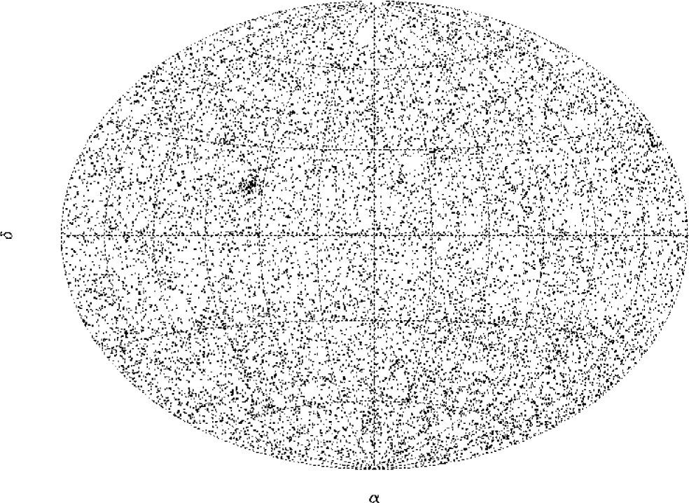
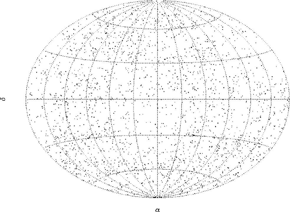
Figure 1: Distribution on the sky of the 16,682 programme stars. Top: The 14,139 stars with radial velocity data (note the overdensity of stars in the Hyades cluster and south of $\delta=-26\degr$). Bottom: The 2,543 stars with no radial velocity.

2.2 Sample definition for the catalogue

The sample of stars for which radial velocities have been obtained was defined from the complete FG catalogue. Slightly generous limits in photometry space have been adopted to allow a selection of FG dwarf stars based on physical criteria like mass, temperature, metallicity, etc.

The following four samples were selected, merged, and cleaned of duplicate entries:

1. All stars for which the F-star calibrations of Crawford (1975) and Olsen (1988) are valid.

2. All stars with no $\beta$ value and 0.240 $\leq b-y\leq$ 0.460, $[m_{1}]\geq$ 0.120, $\delta c_{1}\leq$ 0.400, and $V\leq$ 9.600

3. All stars with 0.205 $\leq b-y\leq$ 0.240, $[m_{1}]\geq$ 0.120, $\delta c_{1}\leq$ 0.400, and $V\leq$ 9.600.

4. All stars for which the G- and K-star calibrations of Olsen (1984) are valid.

Criterion 3 ensures that no metal poor F-stars will be lost on the hot side of the F-type stars. Both criterion 2 and 3 compensate for some missing $\beta$ observations. Criteria 1 and 4 and the $V$-limit 9.6 ensure that a number of fainter stars observed for calibration purposes are also included. After removal of a few known supergiants and other irrelevant objects, the list contains a total of 16,682 objects.

The distribution of the full sample of 16,682 stars over the sky is shown in Fig. 1, in equatorial coordinates and in an equi-area projection. Note the concentration of stars in the Hyades – observed with special care for calibration purposes – and the addition of the latest-type dwarfs south of $\delta=-26\degr$. Apart from these features, the sample is very uniformly distributed on the sky.

3 Observational data

For reference, we summarise in the following the basic observational data underlying the astrophysical and kinematical parameters derived for the programme stars. Our new radial-velocity observations are described in detail; for other data, the relevant sources are given.

3.1 Strömgren $uvby\beta$ photometry

The merged catalogue of $uvby\beta$ photometry from which our programme stars were selected was briefly described above (Sect. 2.2); much additional explanation and extensive notes are given in the original catalogues (Olsen eho83 (1983, 1993); 1994a ; 1994b ). With time, the $\beta$ observations were extended to include all stars with a b-y value indicating that $\beta$ might be a useful reddening-free temperature indicator, except that $\beta$ observations for a small fraction of the northern sky are still pending. The distribution of the sample in b-y colour is shown in Fig. 2.

Figure 2: Distribution of the whole sample in b-y colour.

3.2 Radial velocities

When the first phase of this project was initiated, not even the Bright Star Catalog (Hoffleit & Jaschek bsc82 (1982)) had complete radial-velocity coverage. Of the $\sim$1,500 missing southern stars in that catalogue, the early-type half were observed with conventional spectrographic techniques (Andersen & Nordström 1983a ; 1983b ; Nordström & Andersen na85 (1985)), the late-type half with CORAVEL (Andersen et al. jaetal85 (1985); see also Sect. 3.2.1).

For the fainter stars, new observations were obtained as detailed below – altogether, a total of 62,993 new radial-velocity observations of 13,464 programme stars. Adding earlier literature data, complete kinematical information is available for a total of 14,139 stars.

3.2.1 CORAVEL observations

The bulk of the radial-velocity data presented here was obtained with the photoelectric cross-correlation spectrometers CORAVEL (Baranne et al. baranne79 (1979); Mayor mayor85 (1985)). Operated at the Swiss 1-m telescope at Observatoire de Haute-Provence, France, and the Danish 1.5-m telescope at ESO, La Silla, the two CORAVELs cover the entire sky between them, and their fixed, late-type cross-correlation template spectra efficiently match the spectra of the large majority of our programme stars.

Initially, specific observing programmes were targeted to primarily cover the thick-disk stars which were assumed to be very old, and the evolved thin-disk stars for which ages can be determined. When a separate programme to observe all the late-type southern stars of the Hipparcos survey was initiated (Udry et al. udryetal97 (1997)), most of the remaining southern unevolved F stars were included as well. Subsequently, a good fraction of the northern half of the stars has been also observed in a separate Geneva programme on the Hipparcos stars.

In all programmes, two or more observations were made for almost all stars over a substantial time base. This allows to define more reliable mean velocities, but also to identify most of the spectroscopic binaries which, if unrecognised, yield misleading astrophysical parameters from the observed magnitudes and colour indices. Between the two telescopes, a total of 60,476 CORAVEL observations have been made of 12,941 of the programme stars discussed in this paper - some 1,000 nights’ worth of data.

The catalogue presented here contains the mean radial velocity for each star together with the summary data on the observations as described in the Appendix. Our computations of the observational errors, criterion for detecting variable (i.e. binary) stars, and our treatment of double-lined binaries are discussed in Sect. 3.2.4 below.

Many stars on the main programme are primaries of close double stars. CORAVEL observations were made of the fainter companions to many of these stars in order to ascertain whether they are physically bound or merely optical pairs. These data will be made available separately and are not discussed further here.

3.2.2 CfA observations

The fixed-resolution CORAVEL mask is optimised for sharp-lined spectra, and the cross-correlation profile rapidly becomes too broad and shallow to yield accurate radial velocities for stars rotating faster than 40-50 km s^-1, as is the case for a large fraction of stars with 0.20 $\leq b-y\leq$ 0.27.

In order to recover as many as possible of the early F stars of the sample, several hundred stars rotating too rapidly for CORAVEL were observed with the digital spectrometers (Latham dwl85 (1985)) of the Harvard-Smithsonian Center for Astrophysics (CfA). These instruments yield accurate results for single stars with rotational velocities up to $\sim 120$ km s^-1 (Nordström et al. bnetal94 (1994)) and also perform well on double-lined spectra with two-dimensional cross-correlation techniques (Latham et al. dmvir96 (1996)).

CfA radial velocities for 595 stars were published by Nordström et al. (1997b ) and have been used in the present catalogue when CORAVEL data were missing or less accurate (2,517 observations of 523 stars). Rapidly rotating stars south of declination -40$\degr$ cannot be reached by the CfA instruments and thus have no new radial-velocity data.

Figure 3: Distribution of the mean errors of the mean radial velocities in the catalogue ($top$), and the time span covered for each star ($bottom$).

3.2.3 Literature data

When this programme was initiated, radial-velocity data existed in the literature essentially only for stars in the Bright Star Catalog. As the earlier data were mostly of reasonably good quality, these bright stars have generally not been reobserved. Literature data for a total of 675 such stars and others not covered by the new programmes have been taken, as far as possible, from the compilation of Barbier-Brossat & Figon (2000), and bring the total number of stars with radial velocity data to 14,139.

3.2.4 Variability criterion and binary detection

Each radial-velocity observation is associated with an internal error estimate, $\epsilon$, while an external error estimate is provided by the standard deviation, $\sigma$, of repeated observations at different epochs. From these and the number of observations, $n$, the probability $P(\chi^{2})$ that the observed scatter is due to measuring errors alone may be computed as described in greater detail by Andersen & Nordström (1983b ). $P(\chi^{2})<0.01$ is adopted as our criterion for certain velocity variability – mostly due to binary orbital motion – for both the CORAVEL and CfA data.

Normally, the mean error of the mean radial velocity is computed as $\sigma*n^{-1/2}$. However, if fortuitous good agreement between a few observations results in $\sigma<\epsilon$, then $\epsilon*n^{-1/2}$ is given instead as a more realistic estimate of the mean error of the average velocity.

Occasionally, a double correlation peak may identify a spectroscopic binary from just a single observation, but normally two or more observations are available. In such cases, the centre-of-mass velocity and the mass ratio of a double-lined binary may be computed by the method of Wilson (olinw41 (1941)) without a full orbital solution, if the velocities can be properly assigned to the two components. For the 510 systems for which this has been possible, the systemic velocity is given instead of the raw average of the observations, and the mass ratio is given in Table 2 (electronic form only). The binary population of the sample is further discussed in Sect. 5.1.

Fig. 3 shows the distribution of the mean errors of the mean radial velocities in the sample (upper panel), and of the time span covered by the observations of each star (lower panel). As will be seen, the mean error of a mean radial velocity is typically $\sim$0.25 km s^-1 and only rarely exceeds 1 km s^-1. The observations typically cover a time span of 1-3 years, but occasionally extend over more than a decade.

3.3 Rotational velocities

For stars with significant rotation, the width of the cross-correlation profile is a good indicator of $v$sin$i$. For the stars with CORAVEL observations, $v$sin$i$ has been computed using the calibrations of Benz & Mayor (benzm80 (1980, 1984)). For the CfA observations, the $v$sin$i$ of the best-fitting template spectrum is a good measure of the rotation of the programme star (Nordström et al. bnetal94 (1994); 1997b ).

For the slowest rotators, more elaborate procedures are needed to derive very accurate rotational velocities; for the fastest rotators, the shallow cross-correlation profiles yield results of low accuracy. Accordingly, $v$sin$i$ as derived from the observations are only given to the nearest km s^-1, and from 30 km s^-1 and upwards only to the nearest 5 or 10 km s^-1. As seen in Fig. 4, the great majority of the programme stars have rotations below 20 km s^-1.

Figure 4: Distribution of rotational velocities in the sample.

3.4 Parallaxes

Good distances are crucial in order to compute accurate absolute magnitudes, space motions, and parameters derived from them. Trigonometric parallaxes, generally of very good accuracy, are available from Hipparcos for the majority of our relatively nearby programme stars (ESA hipp97 (1997)). Fig. 5 shows the distribution of the parallaxes ($\pi$) and their relative errors ($\sigma_{\pi}/\pi$); most are better than 10%, nearly all better than 20%. The computation of distances for all our stars is discussed in Sect. 4.4.

Figure 5: Distribution of Hipparcos parallaxes ($top$) and their relative errors ($bottom$) for the whole sample.

3.5 Proper motions

Accurate proper motions are available for the vast majority of the stars from the Tycho-2 catalogue (Høg et al. tycho2 (2000)). This catalogue is constructed by combining the Tycho star-mapper measurements of the Hipparcos satellite with the Astrographic Catalogue based on measurements in the Carte du Ciel and other ground-based catalogues. By this procedure the baseline for determining proper motions is extended up to nearly a century, against only 3.5 years for the Hipparcos mission itself.

For a few stars, mostly very bright stars or close binaries without a Tycho-2 proper motion, a Hipparcos or Tycho measurement has been used instead. The typical mean error in the total proper motion vector is 1.8 milliarcsec/year, corresponding to a mean propagated error in the space velocity of 0.7 km s^-1 from the proper motions alone (i.e., neglecting parallax and radial-velocity errors).

4 Derived astrophysical parameters

In order for the stellar data to be useful in discussing the evolutionary history of the Solar neighbourhood, a number of astrophysically interesting parameters must be derived from the raw observational data. In most cases, calibrations of the photometric indices in terms of intrinsic parameters are found in the literature, except as noted below. We discuss each calibration in turn in the following.

4.1 Interstellar reddening

E(b-y) can be computed for F stars with $\beta$ observations from the intrinsic colour calibration by Olsen (eho88 (1988)). It has been applied in the photometric temperature and distance determinations if E(b-y) $\geq$0.02 and the distance is above 40 pc; otherwise the stars are assumed to be unreddened. Most stars with no value of E(b-y) are late-type dwarfs within 40 pc, which will have negligible reddening anyway. As seen in Fig. 6, very few of the stars have E(b-y) $>$ 0.05 mag. We note that E(b-y) may be overestimated for the hottest, brightest, and most distant early F stars (Burstein burst03 (2003)).

Figure 6: Distribution of reddening values in the sample.

4.2 Effective temperatures

Effective temperatures for all the programme stars have been determined from the reddening-corrected $b-y,$ $c_{1}$, and $m_{1}$ indices and the calibration of Alonso et al. (alonso96 (1996)) which is based on the infrared flux method. The resulting temperatures have been compared to the determinations by Barklem et al. (barklem02 (2002)), based on a fit to the Balmer line wings using the latest broadening theory. The agreement is excellent, with a mean difference of only 3 K and a dispersion of 94 K. We have also compared our results to the spectroscopic excitation temperatures determined by Bensby et al. (bensby03 (2003)) for 63 of our stars; the latter are on average 93 K higher than ours, with a dispersion around the mean of only 57 K. The distribution of the effective temperatures in the sample is shown in Fig. 7.

Figure 7: Distribution of the sample in $T_{eff}$.

4.3 Metal abundances

The accurate determination of metallicities for F and G stars is one of the strengths of the Strömgren $uvby\beta$ system. Among the available calibrations, we have used that by Schuster & Nissen (schuni89 (1989)) for the majority of the stars. In our sample, $\sim$600 stars are covered by both the F and G star calibrations of Schuster & Nissen (schuni89 (1989)), and the mean difference in [Fe/H] is 0.06 with a dispersion around the mean of only 0.07. We have further compared these photometric metallicities with the homogeneous spectroscopic values for F and G stars by Edvardsson et al. (edv93 (1993)) and Chen et al. (chenyq00 (2000)). The agreement is excellent, with mean differences of only 0.02 and 0.00 dex and dispersions around the mean of 0.08 and 0.11, respectively. A further comparison with the compilation by Taylor (taylor03 (2003)) shows a mean difference of only 0.01 dex, but a larger dispersion of 0.12 dex, as expected for a compilation from many sources of varying quality.

Within the range of validity of the Schuster & Nissen (schuni89 (1989)) calibration, we thus find the photometric metallicities to have no significant zero-point offset and remarkably small dispersion when compared to high-quality spectroscopic values. However, as pointed out most recently by Twarog et al. (twarog02 (2002)), the Schuster & Nissen (schuni89 (1989)) calibration seems to give substantial systematic errors in the metallicity computed for the very reddest G and K dwarfs ($b-y>0.46$), where very few spectroscopic calibrators were available at that time. Because our sample contains an appreciable number of such red stars and more spectroscopic metallicities in this range have become available, we decided to derive an improved metallicity calibration for these stars, as follows:

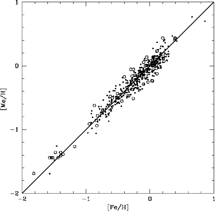
Figure 8: Comparison between our final photometric metallicities ([Me/H]) and the spectroscopic ([Fe/H]) values used to establish the calibrations. Open circles denote the cool (GK) stars, dots the hot (F) stars (see text).

From the high-resolution spectroscopic studies of Flynn & Morell (flynnmo97 (1997)), Tomkin & Lambert (tomkin99 (1999)), Thorén & Feltzing (thoren00 (2000)), and Santos et al. (santos01 (2001)), we have extracted metallicities for 72 dwarf stars in the colour range 0.44 $\leq b-y\leq$ 0.59 and performed a new fit of the $uvby$ indices to these values, using the same terms as the Schuster & Nissen (schuni89 (1989)) G-star calibration. The resulting calibration equation is:

$[Fe/H]=-2.06+24.56m_{1}-31.61m_{1}^{2}-53.64m_{1}(b-y)\\ \leavevmode\nobreak\ \leavevmode\nobreak\ \leavevmode\nobreak\ +73.50m_{1}^{2}(b-y)+[26.34m_{1}-0.46c_{1}-17.76m_{1}^{2}]c_{1}$

The fit of the photometric metallicities from this calibration to the spectroscopic reference values is shown in Fig. 8 (open circles). The dispersion around the (zero) mean is 0.12 dex.

Spectroscopic abundances for such cool dwarfs remain affected by both observational and theoretical uncertainties (see, e.g. Thorén & Feltzing thoren00 (2000)). However, the determinations selected here seem to represent the current state of the art, and we have used our new calibration to compute photometric metallicities for the $\sim$1500 stars in our sample with $b-y>$ 0.46. For the $\sim$600 stars in the interval $0.44<b-y<0.46$, the new calibration agrees with that by the Schuster & Nissen (schuni89 (1989)) to within 0.00 dex in the mean, with a dispersion of 0.12 dex.

About 2400 of our stars with high temperatures and low gravities are outside the range covered by the Schuster & Nissen (schuni89 (1989)) calibration. For these stars we have adopted the calibration of $\beta$ and $m_{1}$ by Edvardsson et al. (edv93 (1993)), when valid. For the stars in common, the two calibrations agree very well (mean difference of 0.00 dex, dispersion only 0.05). For stars outside the limits of both calibrations, we have derived a new relation, using the same terms as Schuster & Nissen (schuni89 (1989)) for F stars. In addition to the above new spectroscopic sources, we used Burkhart & Coupry (burkhart91 (1991)), Glaspey et al. (glaspey94 (1994)) and Taylor (taylor03 (2003)) to extend the coverage in b-y, $m_{1}$, $c_{1}$, and [Fe/H]. From 342 stars in the ranges: 0.18 $\leq b-y\leq$ 0.38, 0.07 $\leq m_{1}\leq$ 0.26, 0.21 $\leq c_{1}\leq$ 0.86 and -1.5 $\leq[Fe/H]\leq$ 0.8, we derive the following calibration equation:

$[Fe/H]=9.60-61.16m_{1}+81.25m_{1}(b-y)\\ \leavevmode\nobreak\ \leavevmode\nobreak\ \leavevmode\nobreak\ \leavevmode\nobreak\ \leavevmode\nobreak\ \leavevmode\nobreak\ \leavevmode\nobreak\ \leavevmode\nobreak\ \leavevmode\nobreak\ +224.65m_{1}^{2}(b-y)-153.18m_{1}(b-y)^{2}\\ \leavevmode\nobreak\ \leavevmode\nobreak\ \leavevmode\nobreak\ \leavevmode\nobreak\ \leavevmode\nobreak\ \leavevmode\nobreak\ \leavevmode\nobreak\ \leavevmode\nobreak\ \leavevmode\nobreak\ +[12.23-90.23m_{1}+38.70(b-y)]\log(m_{1}-c_{3}),$

where $c_{3}=0.45-3.98(b-y)+5.08(b-y)^{2}$.

Figure 9: Distribution of metallicities for the whole sample (full histogram). For comparison, the dotted curve shows a Gaussian distribution with mean of -0.14 and dispersion of 0.19 dex, covering the same area as the histogram.

The fit of these photometric metallicities to the spectroscopic values is shown in Fig. 8 (dots); the dispersion around the relation is 0.10 dex. For the stars in common, the new calibration and that by Schuster & Nissen (schuni89 (1989)) again agree very well (mean difference 0.02 dex, dispersion only 0.04). More detail on the new calibration is given by Holmberg (holmb04 (2004)).

The distribution of the photometric metallicities derived as described above is shown in Fig. 9. A Gaussian curve (with a mean of -0.14 and a dispersion of 0.19 dex) has been plotted to highlight the tail of metal-poor stars in the real distribution. This metallicity distribution for F- and G-type dwarfs is almost identical to the one found for K-type giants by Girardi & Salaris (2001), with a mean of -0.12 and a dispersion of 0.18 dex.

4.4 Distances and absolute magnitudes

Most of our programme stars are nearby and have trigonometric parallaxes of excellent quality from Hipparcos (see Sect. 3.4 and Fig. 5). We have therefore chosen to first determine distances for our stars based on the Hipparcos parallaxes, either directly or indirectly. The distances are used to compute tangential space motion components from the proper motions, and absolute magnitudes used in the determination of ages and masses.

When the Hipparcos parallax is either unavailable or less accurate, a photometric parallax is used. We have adopted the distance calibrations for F and G dwarfs by Crawford (craw75 (1975)) and Olsen (eho84 (1984)); if both are valid for the same star, the F star calibration is preferred (Note that this calibration requires a $\beta$ value). We have checked the photometric distances against the subset of Hipparcos parallaxes with relative errors below 3% (Fig. 10). The trigonometric and (distance independent) photometric parallaxes agree very well, with no significant colour-dependent bias: The photometric distances have an uncertainty of only 13%.

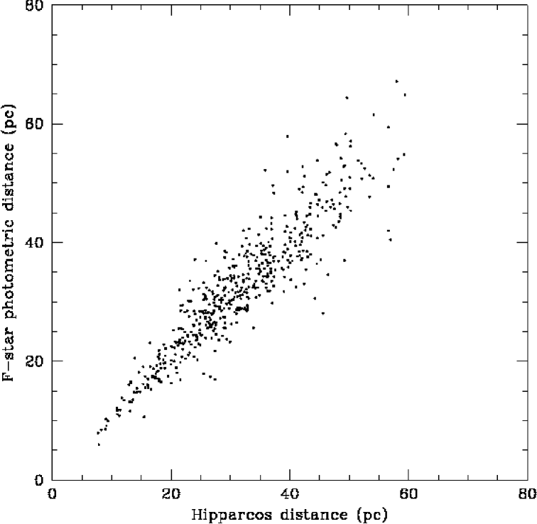
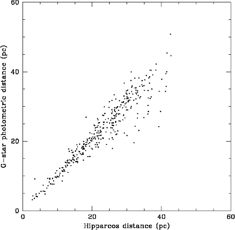
Figure 10: Photometric vs. Hipparcos distances for the single main sequence stars with parallax errors below 3%. Top: F dwarfs; bottom: G dwarfs.

Accordingly, the Hipparcos distance is adopted if the parallax is accurate to 13% or better; otherwise we adopt the photometric distance. However, the photometric distance calibrations are not valid for binaries, giants, and many kinds of peculiar stars. Such stars reveal themselves by large discrepancies between the trigonometric and photometric distance estimates. The (few) stars with photometric distances deviating more than $3\sigma$ from the Hipparcos distances are flagged in the catalogue as suspected binaries or giants, and no photometric distance is given if the Hipparcos parallax is too inaccurate as a distance indicator on its own (235 stars). Similarly, no distance is given for stars which lack the necessary photometry (typically the $\beta$ index) and/or reliable Hipparcos parallaxes or fall outside the photometric calibrations (1214 stars). These stars are all quite distant and of marginal relevance to the overall sample.

From the adopted distances and the observed $V$ magnitudes we have computed the absolute magnitudes given in the catalogue, correcting for interstellar extinction when known. Moreover, a $\delta M_{V}$ index has been calculated as the magnitude difference between the star and the theoretical ZAMS at the same colour and metallicity, as an indicator of the degree of evolution of each star. Fig. 11 shows the distribution of $M_{V}$ and $\delta M_{V}$ values for the sample.

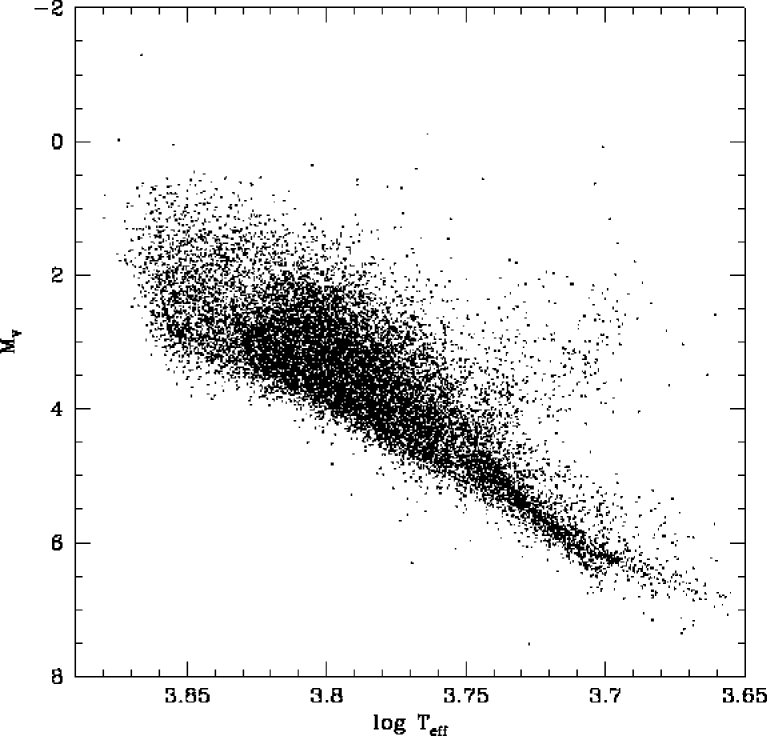
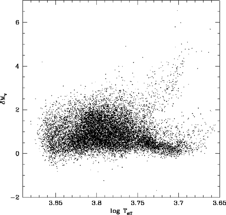
Figure 11: $M_{V}$ ($top$) and $\delta M_{V}$ ($bottom$) vs. $\log T_{eff}$ for our sample, which by design consists of F and G dwarf stars.

4.5 Ages

Individual stellar ages are crucial in order to place the observed chemical and kinematical properties of the stars in an evolutionary context. Because of their importance, we have devoted a great deal of effort to finding the most reliable way to determine ages for the stars in our sample and assessing their individual and systematic errors.

We start by noting that observable diagnostics of stellar ages are basically: (i): chromospheric activity, and (ii): evolution away from the ZAMS in the HR diagram. Both have strengths and limitations, as discussed recently by Lachaume et al. (lachaume99 (1999)) and Feltzing et al. (feltz01 (2001)).

Chromospheric age determinations rely on the decline of stellar activity with time (see Soderblom et al. soderb91 (1991) for an overview). The strength of this technique is that it can be used for both F, G, and K-type dwarfs, including very young stars. A drawback is that the chromospheric activity indicators (e.g. X-ray and Ca II emission) decay into invisibility at about the age of the Sun, so the method cannot be used for the older stars which are of main interest for Galactic evolution. A more basic problem is the time variability of stellar activity, similar to the activity cycles and more dramatic phenomena of the Sun, such as the Maunder minimum. Further, stellar activity is caused mainly by rotation, which decreases with age but can be influenced by, e.g. tidal interaction in binary systems (Kawaler 1989). A chromospheric age can therefore be completely wrong for reasons that cannot be clarified without additional (substantial) observational data.

Isochrone ages are determined by placing the stars in the theoretical HR diagram (Fig. 11), using the observed $T_{eff}$, $M_{v}$, and [Fe/H] and reading off the age (and mass) of the stars by interpolation between theoretically computed isochrones. Edvardsson et al. (edv93 (1993)) exemplify this technique in the present context. Given the presence of observational errors, isochrone ages can only be determined for stars that have evolved significantly away from the ZAMS, where all the isochrones converge. This precludes the determination of reliable isochrone ages for unevolved (i.e. relatively young) stars, and also for G and K dwarfs which evolve along the ZAMS for the first long period of their life.

Many of our stars are considerably older than the Sun. Moreover, chromospheric activity indicators exist only for a small fraction of them. Accordingly, we have chosen to derive isochrone ages for our stars, recognising that meaningful results will not be possible for all our stars.

4.5.1 Selection of stellar models

Selecting an appropriate set of theoretical evolution models and verifying its correspondence with the observed stars is the first crucial step in any determination of isochrone ages. The youngest stars in our sample are massive enough that the stellar models must incorporate convective core overshooting where appropriate. Several such models exist and are, in fact, very similar in the theoretical plane, but employ rather different transformations to the standard colour systems (see, e.g., the detailed comparison in Nordström et al. 1997a ). We have preferred, therefore, to compute effective temperatures and luminosities for the programme stars and compare with the models directly in the $\log T_{eff}-M_{v}$ plane.

In preparation, we have compared the latest models from both the Geneva (Mowlavi et al. nami98 (1998); Lejeune & Schaerer lejeune01 (2001)) and Padova groups (Girardi et al. girardi00 (2000), Salasnich et al. salasn00 (2000)). The two sets of models yield essentially the same ages (to within 10%), but have significant and different limitations for our purposes: The Geneva models extend to very large ages, but are computed for a relatively coarse grid of masses $\geq 0.8M_{\odot}$, which precludes a proper determination of masses and ages for our coolest dwarf stars and leads to some numerical problems in the detailed isochrone interpolations. The Padova models extend to stars well below the lower mass limit of our sample, but the isochrones are terminated at an age of 17.8 Gyr, complicating the proper computation of mean ages and age errors for the oldest stars in our sample. Ages much in excess of 17.8 Gyr exceed all recent estimates of the age of the Universe, however, so on balance, we have chosen the Padova models for the final age determination.

4.5.2 Choice of model compositions

The next issue concerns the choice of chemical composition for the models. It has long been known (e.g Edvardsson et al. edv93 (1993), Reddy et al. reddy03 (2003)) that disk stars with [Fe/H] $<$ 0 exhibit an average enhancement of the $\alpha$-elements which rises approximately linearly to [$\alpha$/Fe] $\simeq+0.25$ at [Fe/H] = -1 and remains constant at that or perhaps a slightly higher level in even more metal-poor stars. The total heavy-element content of metal-deficient disk stars is thus somewhat higher than the heavy-element content of the Sun scaled by the observed [Fe/H].

Moreover, recent work (e.g. Fuhrmann fuhrm98 (1998), Bensby et al. bensby03 (2003)) has found that thick-disk stars appear somewhat more $\alpha$-enhanced than thin-disk stars in the range $-1<$ [Fe/H] $<0$, which spans the vast majority of our sample. There is, however, no consensus on a precise criterion to distinguish between stars of the thin and thick disks, in particular whether thick-disk stars are all extremely old and/or all moderately metal-poor. This makes it impractical to identify the $\sim 5\%$ thick-disk stars and estimate separate $\alpha$-enhancements for thin- and thick-disk stars. Moreover, while Padova isochrones are available for the Solar mixture of heavy elements as well as with an enhanced $\alpha$-element content for some values of [Fe/H], the assumed $\alpha$-enhancement ([$\alpha$/Fe] $\simeq+0.35$) is considerably greater than appropriate for most of our stars.

Fortunately, a simpler procedure appears sufficient. As demonstrated most recently by VandenBerg (davb00 (2000)), isochrones computed with solar-scaled and $\alpha$-enhanced compositions are almost indistinguishable, provided the total heavy-element content $Z$ remains constant. For the metal-poor stars, we therefore select scaled-Solar composition Padova isochrones with a somewhat higher [Fe/H] than the directly observed value, as described below.

Specifically, we assume an $\alpha$-enhancement that is zero for Fe/H] $\geq 0$, rises linearly with decreasing [Fe/H] to +0.25 dex at [Fe/H] = -1.0 and +0.4 dex at [Fe/H] = -1.6, then remains flat at +0.4 dex at all lower metallicities. Following VandenBerg (davb00 (2000)), we then increase the observed [Fe/H] by 75% of the corresponding value of [$\alpha$/Fe] as the best estimate of the total heavy-element content of each star. We note that VandenBerg (davb00 (2000)) found his procedure to be less satisfactory for the most metal-rich compositions, but those results were derived for a constant [$\alpha$/Fe] = +0.3 dex, even for [Fe/H] $>0$. The above approximation should remain fully satisfactory in the slightly metal-poor regime with the far smaller $\alpha$-enhancements adopted here.

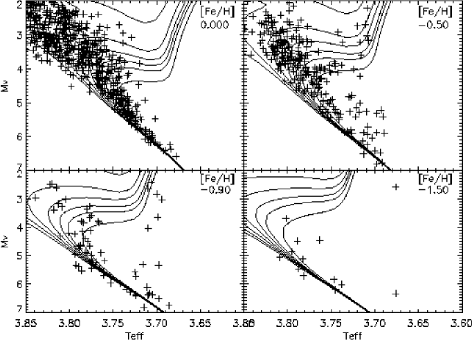
Figure 12: Comparison between the observed stars (known binaries excluded) and Padova isochrones for 0, 2, 4, 6, 8, 10, and 15 Gyr at [Fe/H] = $0.00\pm 0.02$, $-0.50\pm 0.05$, $-0.90\pm 0.20$, and $-1.50\pm 0.25$, after allowing for the $\alpha$-enhancement and temperature corrections discussed in the text.

4.5.3 Adjusting the temperature scales

Having described our procedure for choosing models of appropriate heavy-element content for stars of different metallicity, we ask whether these models provide a satisfactory fit to the observed stars. This is especially important for the effective temperatures, which are notoriously difficult to predict in an absolute sense from stellar models as well as from observation (see, e.g. Lebreton lebreton01 (2001)). A temperature mismatch between the models and observed stars will enter directly into the derived ages.

Because our sample is expected to include very old stars, the comparison must be made on the unevolved main sequence, i.e. for $M_{v}>$ +5.5. Good agreement is found for Solar and very metal-poor compositions, but for intermediate values of [Fe/H] the models are too hot by small, but significant amounts, as also found by Lebreton (lebreton01 (2001)). Ignoring this offset would drive the low-mass stars to spuriously high ages, given the tight spacing of the isochrones in this mass range.

Accordingly, we have applied temperature corrections to the models that amount to a $\delta\log T_{eff}$ of -0.015 at [Fe/H] = -1.5, rising linearly to $\delta\log T_{eff}$ = -0.022 at [Fe/H] = -1.0 and dropping linearly again to zero at [Fe/H] = -0.3. With these corrections, we obtain the isochrone fits to the lower main sequence shown in Fig. 12, which we consider satisfactory.

4.5.4 Statistical biases in age determinations

The classical way to determine an isochrone age is to plot the observed stars and computed isochrones together in the theoretical HR diagram, either the $\log T_{eff}-M_{V}$ diagram (Fig. 11, top) or the $\log T_{eff}$ vs. $\delta M_{V}$ variety (Fig. 11, bottom) used by Edvardsson et al. (edv93 (1993); see their Figs. 10-11). Errors are then derived by varying each of the independent variables $\log T_{eff}$, $M_{V}$, and [Fe/H] by their estimated observational errors and noting the changes in the resulting age.

However, age is a highly non-linear function of position in the HR diagram; the distribution of the observed parameters is highly non-uniform as well; and the observational errors are not always negligible compared to the ranges over which these distributions and the derived ages vary considerably. An age probability distribution function computed without regard to these effects will therefore be biased; moreover, in the simple, “classical” approach it is also incompletely sampled. Biased ages and misleading error estimates are the likely result.

Statistical biases effecting the determination of isochrone ages include the following:

1. Stellar evolution accelerates strongly when stars leave the main sequence; therefore, the density of stars in the HR diagram will be much higher in the main-sequence region than away from it. This, in turn, causes more stars to be scattered by observational errors from the main sequence into the subgiant region than the reverse, and leads to a bias in favour of high ages. Note that this effect is in fact exacerbated if stars with poorly determined ages are eliminated, since unevolved stars necessarily have poorly-determined ages.

2. Standard initial mass functions (IMF) rise towards lower stellar masses; a given isochrone will therefore not have equal numbers of stars in equal mass steps, but the density of stars will rise towards the ZAMS. Ignoring this effect will also lead to a positive age bias.

3. Standard disk metallicity distributions (see Sect. 6.1) contain many more metal-rich than metal-poor stars; observational errors will therefore again scatter more stars from the metal-rich peak of the distribution into the metal-poor tail than in the opposite direction. This will cause the corresponding ages to be derived from isochrones that are too metal-poor, i.e. too hot, and again a positive age bias results (the converse argument applies to the tail of “super metal-rich” stars).

4. Apart from such “intrinsic” effects in the data, the distribution of stars in the HR diagram will be non-uniform because, e.g. of a non-uniform age distribution of the stars themselves, or as a result of the criteria used to define the sample. Notably, the distribution in the HR diagram of our full magnitude-limited sample will be quite different from that of the volume-limited subsample, due to the inclusion of luminous, evolved stars from much larger distances.

4.5.5 Age determination for the sample stars

The techniques we have developed to allow for these biases are superficially similar to those discussed recently by Lachaume et al. (lachaume99 (1999)) and Reddy et al. (reddy03 (2003)) as regards the treatment of the evolution bias referred to above. There are, however, important differences, in that we treat all three parameters $\log T_{eff}$, $M_{V}$, and [Fe/H] equally, include several additional sources of bias, and consider the whole chain of astrophysical links from data to age. Our method is outlined below and described in greater detail by Jørgensen & Lindegren (bjarner04 (2004)).

Briefly, for every point in a dense grid of interpolated Padova isochrones we compute the probability $P$ that the star could in reality be located there (and thus have the corresponding age), given its nominal position in the three-dimensional HR “cube” defined by $\log T_{eff}$, $M_{V}$, and [Fe/H]. To do so, we assume that the associated observational errors have a Gaussian distribution:

$P=\exp(-(\Delta T_{eff})^{2}/2\sigma_{T_{eff}}^{2})*\exp(-(\Delta M_{v})^{2}/2\sigma_{M_{v}}^{2})*\\ \leavevmode\nobreak\ \leavevmode\nobreak\ \leavevmode\nobreak\ \leavevmode\nobreak\ \leavevmode\nobreak\ \leavevmode\nobreak\ \leavevmode\nobreak\ \leavevmode\nobreak\ \leavevmode\nobreak\ \leavevmode\nobreak\ \leavevmode\nobreak\ \exp(-(\Delta[Fe/H])^{2}/2\sigma_{[Fe/H]}^{2})$

Here, $\Delta T_{eff}$ etc. are the differences between the observed parameters of the actual star and the isochrone points considered. We assume constant errors ($\sigma$) of 0.01 dex in $\log T_{eff}$ and 0.1 dex in [Fe/H] throughout; for $M_{V}$ we use the individual error estimate if an Hipparcos parallax better than 13% exists; otherwise, the standard photometric value of 0.28 mag in (m-M) is adopted.

Integrating over all points gives the global likelihood distribution for the possible ages of the star, conditioned to account for observational biases as described below. We call this the “G-function” and normalise it to unity at maximum. The most probable age for the star is then determined as the value for which the G-function has its maximum (see Fig. 13).

Figure 13: Top: Three slices of the three-dimensional HR “cube” showing the observed point (central panel) and three cuts through the 1-$\sigma$ error ellipsoid. The probability distribution function (G-function, bottom) is computed from $all$ points on the isochrones, not just those on or inside the error ellipsoid.

The determination of the maximum value itself is a non-trivial task. Because of numerical noise due to the finite sampling of the isochrones, a simple maximum of the raw function results in spurious high-frequency features in the derived age distributions which go undetected in small samples, but have dramatic effects in densely-populated diagrams such as Figs. 27 and 30. The median of, say, the upper 50% of the function yields a more stable estimate, but if the corresponding age range includes one of the limits (0 or 17.8 Gyr), the estimate will be biased away from the limit, leading to spuriously low ages for the oldest stars (cf. Fig. 14). A Gaussian fit as used by Reddy et al. (reddy03 (2003)) is also more stable, but is a poor approximation in the frequent cases when the G-function is distinctly non- Gaussian (Fig. 14).

After extensive tests with simulated and real data, smoothing the G-function slightly with a kernel depending on the width of the unsmoothed function was found to be the optimum procedure. The maximum of the smoothed function then yields a stable age estimate without significant bias. Fig. 13 illustrates the procedure in the well-behaved case of a star located in a region of the HR diagram where the isochrones are well separated, and the maximum of the G-function yields a well-defined age.

Finally, the maximum value of the probability function found for any point on the isochrones is a measure of the degree to which the star is covered by the models. A small value signifies peculiar stars or large observational errors which preclude any realistic age determination.

In computing the G-functions, we have accounted for the biases described in Sect. 4.5.4 as follows:

1. Speed of evolution. The isochrones are more widely separated in phases of rapid evolution, so such phases automatically receive lower weight in the integrations. We emphasize that not only points within a 1-$\sigma$ (or 3-$\sigma$, Reddy et al. reddy03 (2003)) error ellipse are included, but all points on the isochrones in all three dimensions.

2. Stellar mass function. The varying density of stars on an isochrone towards the main sequence is accounted for by weighting each point according to the IMF (Kroupa et al. kroupa93 (1993)). It can be argued that the slope of the actual distribution in the magnitude-limited sample will be lower than that of the IMF due to the preferential inclusion of brighter, higher-mass stars, but the effect is hard to quantify and in any case small, as the range in masses covered by the sample is small.

3. Metallicity bias. The excess of apparently metal-poor stars caused by observational scatter from the large peak of stars of near-Solar metallicity is straightforward in concept. Allowing rigorously for it in practice is another matter: A fully Bayesian approach requires an estimate of the a priori distribution which is a priori unknown and, moreover, rather different for the complete, magnitude-limited catalogue and for the volume-limited sample which will no doubt be preferred in many applications (compare Figs. 9 and 26); other subsamples would no doubt be different again. It appears unreasonable that the catalogued age of a given star should depend on the subsample of stars discussed together with it.

   Moreover, the first-order astrophysical effects considered earlier in the procedure already seem to allow for these effects. First, if significant, the metallicity bias should appear as an excess of positive residuals at low [Fe/H] when photometric metallicities are compared with spectroscopic determinations; this is not seen in our data (nor by Edvardsson et al. edv93 (1993)). Second, our revised metallicity calibration (see Fig. 8), by design, yields the correct mean spectroscopic [Fe/H] for a given mean photometric metallicity.

   Finally, and probably most importantly in view of the sensitivity of the derived ages to small temperature shifts, the samples of stars used to “normalise” the temperature scale of the models to that of the observed stars (Fig. 12) will already be affected by any residual metallicity bias. Our temperature shifts will therefore allow for it to first order. In fact, it could be argued that these corrections may, if anything, be too large because the stars were drawn from the full, magnitude-limited sample which preferentially includes young, metal-rich stars.

   In summary we believe that, for general use, little if any metallicity bias of significance remains in the ages given in the catalogue. If particularly precise ages are needed for certain types of stars, well-defined subsamples should be extracted and all steps in the analysis reviewed and/or repeated, including the temperature and metallicity calibrations, [$\alpha$/Fe] ratio(s), model compositions and bolometric corrections, and the a priori distributions of the relevant parameters.

4. Age bias etc. A strongly peaked age distribution (e.g. due to a starburst) could give biases analogous to those discussed above. No such peak is expected, and its effects would again depend on the (sub)sample considered. We have also not imposed any upper limit on the derived ages: While true ages greater than $\sim$13 Gyr are implausible, observational error will cause some determinations to exceed this limit, and imposing a cutoff will bias the mean age of the oldest stars.

In cases (1)-(2) we correct for the a priori information in a fully Bayesian manner. Including also a priori metallicity and age distributions in the age determination at this stage would build our prejudices concerning the enrichment and star-formation history of the disk into our age estimates for individual stars. We have therefore not made such corrections to the ages listed in the catalogue (equivalent to assuming flat a priori distributions.)

Using the above procedures, G-functions have been computed for all stars in our sample with the necessary input data, including binary stars etc. An electronic table of these functions, which illustrate the determinacy of each age determination at a glance, will be made available to interested readers by request to the corresponding author (B.R.J.; bjarne@astro.lu.se).

Bayesian probability theory offers an independent, alternative method to compute unbiased age estimates under similar conditions, provided that the a priori distributions of the relevant parameters can be estimated with sufficient accuracy. An end-to-end Bayesian approach of this type is described and applied to the data of Edvardsson et al. (edv93 (1993)) by Pont & Eyer (pont04 (2004)).

4.5.6 Estimating errors for the ages

Realistic error estimates are crucial in any applications of the ages. From a well-behaved G-function such as that shown in Fig. 13 we derive (separate) 1-$\sigma$ lower and upper age limits as the points where the G-function reaches a value of 0.6. Extensive Monte Carlo simulations using artificial stars with typical observational errors have confirmed that indeed 68% of the recovered ages then fall within $\pm 1\sigma$ of the correct age.

When both the upper and lower 1-$\sigma$ age limits fall within the range of the isochrones, 0-17.8 Gyr, the catalogue lists both the most likely age of the star as well as its upper and lower limits. In the following, we refer to such cases as “well-defined” ages (note that this term by itself does not imply a small error, only that the error estimate is reliable!). For more demanding applications, the sample should no doubt be restricted to single stars and perhaps also to stars with age errors below a specified limit; all information needed to do so is readily available in the catalogue.

If the G-function peaks within the valid age range but one of the limits is outside it, that limit is not given in the table, indicating that the age is uncertain and its error also poorly defined. For stars near or beyond the limits of the isochrone set (very young or very old stars with large observational errors, duplicity or other spectral peculiarities), the G-function may peak at or even outside the age limits of the isochrones (see Fig. 14). In such cases, no value is given for the age, only the estimated upper or lower limits.

Figure 14: Right: Examples of stars located in regions of the HR diagram where reliable ages cannot be determined, and (left) the corresponding G-functions. The stars plotted as plus, asterisk, triangle, and diamond symbols in the HR diagram correspond to the solid, dotted, dashed, and dot-dashed curves, respectively. Isochrones are for 0, 2, 4, 6, 8, and 10 Gyr.

Finally, for the lowest-mass stars which have not evolved perceptibly, the G-function will show no well-defined maximum (see Fig. 14). If the G-function is too flat to reach the 1-$\sigma$ confidence level (0.6) anywhere in the range 0-17.8 Gyr, or if the maximum probability value entering the computation of the G-function indicates that the star falls significantly outside the isochrone set, no age is given at all.

Figure 15: The distribution of upper (dotted line) and lower (solid line) 1-$\sigma$ relative errors for the ages in the catalogue.

The distribution of the relative age errors is shown in Fig. 15, while Fig. 16 shows the mean relative age error as a function of age for the stars with “well-defined” ages. Note that the condition that both lower $and$ upper age limits should be determined removes old stars from the upper right in Fig. 16. The impression of increasing precision with age that results when a numerical cutoff is mistaken for a physical upper age limit (e.g. Fig. 4 of Feltzing et al. feltz01 (2001)) is, of course, an illusion.

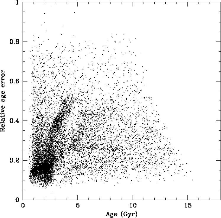
Figure 16: Relative age error (mean of lower and upper bounds) vs. age for the 11,445 stars with “well-defined” ages.

We have compared our error estimates with those derived in the classical manner, i.e. by varying each input parameter by $\pm 1\sigma$ and adding the age errors in quadrature. We find that the latter are often underestimated by almost a factor 2. We attribute this to three causes: (i): Varying only one parameter at a time significantly underestimates the true range of values over which the age variations must be explored; (ii): the technique effectively samples a total of only six points on the three-dimensional probability function which we integrate in detail to compute the G-function; and (iii): the standard way to add errors assumes implicitly that the G-function is Gaussian, which is manifestly not the rule (cf. Fig. 14). Some of the error estimation techniques for isochrone ages in earlier literature have in reality estimated fitting errors rather than true uncertainties, and the errors have likely been significantly underestimated in several cases.

In the total sample of 16,682 stars, these criteria yield age estimates for 13,636 stars (82%), of which 11,445 stars (84%) have “well-defined” ages by the above definition. 9,428 (82%) of these well-defined ages have estimated errors below 50%, 5,472 (47%) even below 25%. Eliminating known binaries of all types leaves us with 9,158 presumably single stars (83% of all 11,060 such stars in the sample) with derived age values, 7,566 (83%) of which have ages that qualify as “well-defined”. Of these in turn, 6,144 single stars (81%) have ages better than 50% and 3,528 (46%) better than 25%, respectively.

Fig. 17 shows the distributions of derived ages for the complete (magnitude-limited) sample for increasingly strict limits on the accuracy of the ages, and also compares the distributions of the magnitude-limited and volume-limited samples. We stress that, due to the biases in the selection and age computation procedures already discussed, none of these diagrams has a simple interpretation in terms of the star formation history of the Solar neighbourhood.

Figure 17: Top: Age distributions for single stars in the full sample. The curves show (top to bottom): (i) all ages (solid); (ii) “well-defined” ages (dots); (iii) ages with errors $<50$% (short-dashed); and (iv) ages with errors $<25$% (long-dashed). Bottom: “Well-defined” ages in the full, magnitude-limited sample (solid) and in the volume-limited subsample for $d<40$ pc (dots). Note that increasing the demand on accuracy progressively removes most of the oldest stars.

4.5.7 Checking the results

We have subjected our age derivation procedures to a wide range of numerical and other checks. In analogy with the Monte Carlo simulations used to verify the error estimates as described above, we have created artificial samples of stars of specified ages and a range of masses from the isochrones, computed $uvby\beta$ indices and $M_{V}$ values using the reverse transformations of those applied to the observed data, and added realistic random errors to the simulated observations. These artificial stars have then been subjected to our age determination procedure in exactly the same manner as the observed stars. We find that, within the limits of the computed errors, we recover the input ages without significant systematic error (but of course with a loss of stars in the parts of the HR diagram where ages cannot be determined).

Another reality check is to determine ages for stars in open clusters with good $uvby$ photometry and known reddening (including, but not limited to such favourable cases as NGC 3680; Nordström et al. 1997a ) as if they were single stars. Again, good agreement is found with the results of detailed isochrone fits to the entire cluster sequence, but of course the unevolved lower main-sequence stars yield large error bars. Similar consistency checks have been made in binary stars with good data for the individual components. Further discussion of these tests is given by Jørgensen & Lindegren (bjarner04 (2004)).

A particular concern was to ensure that our procedure does not introduce metallicity-dependent systematic errors that could distort the resulting age-metallicity relations (AMR). In order to do so, we have created artificial AMRs of specified shape, with a distribution of metallicities at each age corresponding to the observational scatter, and with a uniform distribution of stellar masses from the ZAMS value to the maximum reached for the assigned age and metallicity. For the experiment, we assumed both an AMR with [Fe/H] increasing linearly with time and another (completely unphysical) AMR in which [Fe/H] decreased linearly with time. Simulated observations and realistic errors were computed and ages and metallicities rederived from the artificial data. As before, many stars were lost for which reliable ages could not be determined, but those with small calculated errors delineated the input AMR without any systematic error – a result which inspires confidence in our method. Details on these simulations are given in Holmberg (holmb04 (2004)).

A further external check was made by comparing with the ages by Edvardsson et al. (edv93 (1993)). Of their 182 stars with ages, our procedure yields estimates of any quality for 179 stars and “well-defined” ages (see above) for 160 stars. Fig. 18 compares the two sets of ages for the latter sample; a linear fit yields the relation
$\log Age_{Edv93}=(0.11\pm 0.03)+(0.89\pm 0.04)*\log Age_{our}$.
I.e., our ages are on average slightly smaller than those of Edvardsson et al. (edv93 (1993)) for younger stars (where their $M_{V}$ derived from $\delta c_{1}$ is biased towards brighter values), while our ages agree well for the oldest stars. The scatter around the $45\degr$ line is 0.12 dex; the fit only reduces it to 0.11 dex. Edvardsson et al. (edv93 (1993)) estimated that their ages had errors of about $\pm 0.1$ dex. Our estimated mean relative error for the same sample is also 0.10 dex, somewhat larger for the youngest and smaller for the oldest stars, but the sample excludes the very oldest stars for which an upper age limit cannot be properly determined.

Figure 18: Ages from Edvardsson et al. (edv93 (1993)) vs. our results for the 160 stars in common with “well-defined” ages.

The agreement between our ages and those derived by Edvardsson et al. (edv93 (1993)) is quite gratifying: One would have expected a larger dispersion in Fig. 18 if the errors in the two age determinations were completely uncorrelated, which suggests that the errors are primarily observational rather than systematic. We recall that even though the same photometric data have been used, the stellar models (including opacities and convection descriptions), temperature and metallicity calibrations, absolute magnitude determinations (Hipparcos parallaxes vs. $\delta M_{V}$ derived from the $\delta c_{1}$ index), treatment of the $\alpha$-enhancement in metal-poor stars, and the method for computing the ages have all changed in the intervening decade. Finding a relation such as that seen in Fig. 18 strengthens one’s confidence in the whole procedure.

We have also compared our results with ages computed with the Bayesian method of Pont & Eyer (pont04 (2004)). Apart from a scale difference of $\sim 25$%, due to a different metallicity scale and their choice of the median rather than maximum of the probability distribution as the preferred age, there is no significant difference between, e.g., age-metallicity relations derived with the two sets of ages.

For completeness, we finally compared our new age determinations (with errors $<$25%) with the chromospheric ages derived by Rocha-Pinto et al. (rocha00 (2000)) for the 85 stars in common in the range 1-20 Gyr. The plot is quite similar to Fig. 8 of Feltzing et al. (feltz01 (2001)), with no trace of any correlation between the two sets of ages.

In conclusion, while noting the uncertainties, we consider our age scale to be the best presently available for the whole sample. However, if the age of a particular subgroup of stars, e.g. thick-disk stars, is needed to the highest precision, then the detailed elemental composition of a carefully defined sample of such stars should be determined and models of precisely the same composition be computed to derive their ages.

It must be emphasised that our reliability tests pertain to the ages derived for individual stars. For any realistic distribution of true ages for a complete sample of stars, one must take into account that many of the least-evolved stars, especially the old low-mass stars, will have no derived age in the catalogue, simply because the observations cannot measure their evolution. We caution, therefore, that the true age distribution of the full sample cannot be derived directly from the catalogue; careful simulation of the biases operating on the selection of the stars and their age determination will be needed to obtain meaningful results in investigations of this type.

Finally, we recall that many stars in our sample are binary or multiple systems, for which the derived ages (and metallicities) will be unreliable. In general, there is insufficient information available to recover the data for the individual binary components from the combined photometry, but the great majority of the visual and spectroscopic binaries in the sample are known and identified in the catalogue (see 5.1), and can thus be excluded in studies where absolute statistical completeness is not important.

4.6 Masses

Mass estimates are needed as the main clue to the evolutionary history of the stars in the sample. Because each point on a model isochrone corresponds to a specific mass value as well as an age, we can compute an M-function describing the probability distribution of model masses for an observed star from the Padova models, exactly analogous to the G-functions for the ages (see Sect. 4.5.5).

The M-functions are much better behaved than the G-functions and generally yield good masses also for stars to which no meaningful age can be assigned. Individual error estimates are also given for all masses in the catalogue; they average about 0.05 $M_{\odot}$. Fig. 19 shows the distribution of the derived masses in both the magnitude-limited and volume-limited samples. The low-mass limit at 0.65 $M_{\odot}$ reflects the red colour cutoff of our sample.

Figure 19: The distribution of derived masses for single stars in the full (solid line) and volume-limited sample for $d<40$ pc (dotted line).

4.7 Space velocities

Space velocity components $(U,V,W)$ have been computed for all the stars from their distances, proper motions, and mean radial velocities. $(U,V,W)$ are defined in a right-handed Galactic system with $U$ pointing towards the Galactic centre, $V$ in the direction of rotation, and $W$ towards the north Galactic pole. No correction for the Solar motion has been made in the tabulated velocities. Our radial velocities are of superior accuracy (Fig. 3) and the average error of the Tycho-2 proper motions corresponds to only 0.7 km s^-1 in the tangential velocities, so the dominant source of error in the space motions is the distance. Accounting for all these sources, we find the average error of our space motions to be 1.5 km s^-1 in each component (U, V, and W).

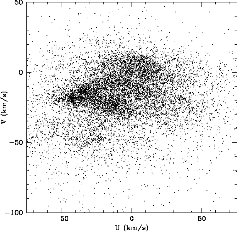
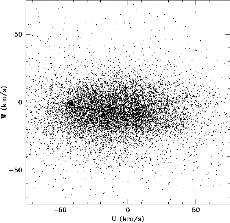
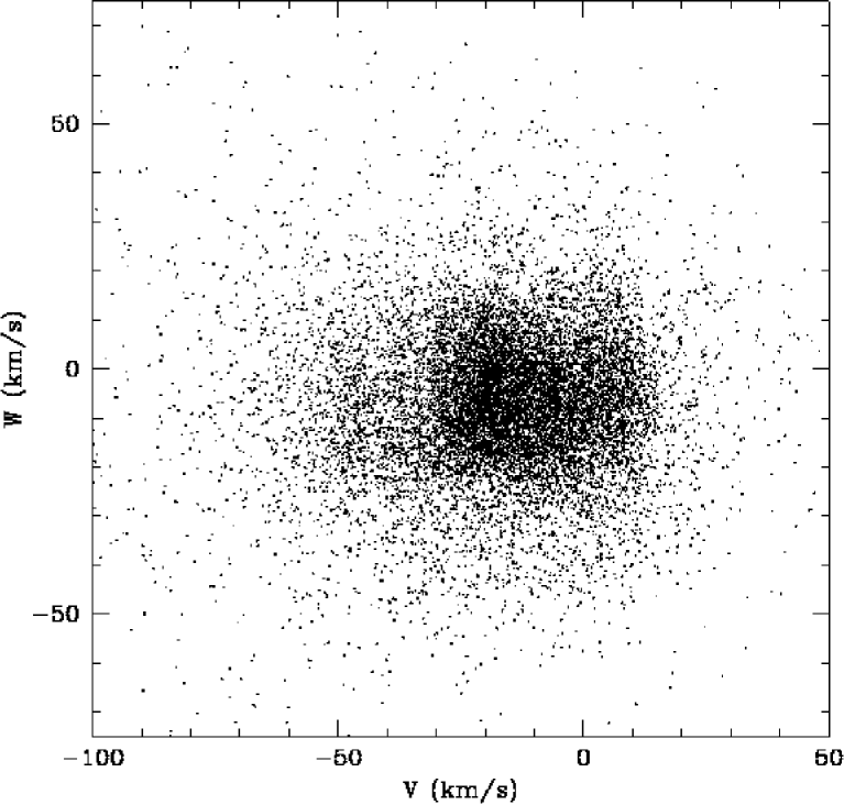
Figure 20: U-V, U-W, and V-W diagrams for all stars in the sample.

Fig. 20 displays (U, V, and W) for all stars in the sample with a measured radial velocity. The U-W and V-W diagrams show a smooth distribution, the Hyades being the only clearly discernible structure (cf. Fig. 1 and Sect. 2.2). The U-V diagram, on the other hand, shows abundant structure in addition to the Hyades, with four curved or tilted bands of stars aligned along approximately constant $V$-velocities. Note that the preponderance of stars from the two nearest spiral arms in our local sample leads to the well-defined limits of these structures seen both in the U-V diagram and in the V-W diagram (at $V$ = -30 and +20 km s^-1).

These structures, discussed e.g. by Dehnen (dehnen98 (1998)), Skuljan et al. (skuljan99 (1999)), have velocities resembling classic moving groups or stellar streams and have been named (top to bottom): The Sirius-UMa, Coma Berenices (or local), Hyades-Pleiades, and $\zeta$ Herculis branches. The location of the $\zeta$ Herculis branch in the U,V plane raises the interesting prospect that kinematically selected samples of local thick-disk stars (e.g. Bensby et al. bensby03 (2003)) might contain an admixture of somewhat younger, more metal-rich thin-disk stars.

Because these structures do not consist of coeval stars (see Fig. 30), they are not simply the remnants of broken-up systems such as classic moving groups, but could be produced by transient spiral arm structures (De Simone et al. desimon04 (2004)) or result from kinematic focusing by non-axisymmetric structures of the Galaxy such as the bar (e.g. Fux fux01 (2001) and references therein). Our data will allow more refined searches for detailed dynamical substructure resulting, e.g., from past merger events (e.g., Chiba & Beers chiba00 (2000), Helmi et al. helmi03 (2003)) or from the dynamical effect of the bar.

4.8 Galactic orbits

From the present positions and space motion vectors of the stars, we can integrate their orbits back in time for several Galactic revolutions and estimate their average orbital parameters. Correlating such Galactic orbits with the chemical characteristics and ages of well-defined groups of stars may yield insight of great interest into their origin; see e.g. Edvardsson et al. (edv93 (1993)) and many later papers.

Before using the observed space motions for this task, they must be transformed to the local standard of rest. For this, we have adopted a Solar motion of (10.0, 5.2, 7.2) km s^-1 (Dehnen & Binney dehnbin98 (1998)). For the orbit integrations we used the potential of Flynn et al. (flynnjsl96 (1996)), adopting a solar Galactocentric distance of 8 kpc. The key properties of this model are: Circular rotation speed 220 km s^-1, disk surface density 52 $M_{\odot}\leavevmode\nobreak\ pc^{-2}$, and disk volume density 0.10 $M_{\odot}\leavevmode\nobreak\ pc^{-3}$, in agreement with recent observational values (Reid et al. reid99 (1999), Backer & Sramek BaSra99 (1999), Flynn & Fuchs flynnfu94 (1994), Holmberg & Flynn holmb00 (2000)).

In the catalogue we give the present radial and vertical positions ($R_{gal}$ and $z$) of each star as well as the computed mean peri- and apogalactic orbital distances $R_{min}$ and $R_{max}$, the orbital eccentricity $e$, and the maximum distance from the Galactic plane, $z_{max}$. Fig. 21 summarises the distribution of these parameters.

The detailed shape of especially the $R_{min}$ distribution is strongly dependent on the exact value of the Solar V-velocity applied, and the peaks can be related to the enhanced density of stars in the streams seen in Fig. 20. Sirius-UMa causes the peak at $\sim$ 8kpc in the $R_{min}$ distribution, Hyades-Pleiades the one at $\sim$ 7kpc, and the small bump at $\sim$ 5.5 kpc can be traced to the $\zeta$ Herculis stream. Tests have shown that an increase of the Solar $V$-velocity by a few km/s changes the double-peaked structure into a smooth increase, due to the changed orbit distribution across the circular velocity.

Figure 21: Key parameters of the Galactic orbits for the whole sample.

5 Statistical properties of the sample

Few if any complete and unbiased samples of stars with complete, homogeneous astrophysical data exist in Galactic astronomy. Indeed, the conclusions of an observational study may well depend more on the way the stars are selected than on the actual data obtained. Thus, for any application of the data presented here it is crucial to be aware of the manner in which the stars have been selected and observed, and how their astrophysical parameters have been derived.

A chief concern at the start of the project was to avoid any kinematic bias in the selection of stars. Therefore, stars for the photometric surveys were originally selected based on the HD visual magnitudes. These are known to have appreciable errors, so some stars brighter than the limits described in Sect. 2.1 will certainly have been missed, while many of the newly measured magnitudes were fainter than those limits. The wide range of HD spectral types included in the surveys should ensure that few if any metal-poor stars were missed from the final (much smaller) sample of F and G dwarfs defined from the measured $uvby\beta$ indices. The cool limit is somewhat less rigorously defined, as old metal-rich dwarf stars might be mistaken for giants because of their strong CN bands, possibly even in the MK spectral classes used to extend the red limit of the sample to K2 V south of $\delta$ = -26$\degr$.

As a practical factor, many of the radial-velocity observations were made from preliminary versions of the photometric catalogues, so the final selection criteria did not necessarily coincide precisely with the way the observations were made. Stars that had already been observed could be excluded in the final sample if needed, but new stars could not necessarily be added. This is the case for a fraction of the unevolved F stars; they had been omitted initially because no reliable ages can be determined for them, and not all were included in the Hipparcos Input Catalogue which was later used to complete the data. Also, several hundred stars yielded no radial-velocity determination because of fast rotation, bright hot companions, or for other reasons.

Inevitably, when many tens of thousands of observations are performed manually on hundreds of nights, occasional misidentifications and other errors occur. The thousands of double stars of all possible varieties provide rich opportunities for ambiguity and inconsistency in the attribution of individual observations. Great effort has been devoted to detecting and eliminating errors of all conceivable kinds, but not all cases can be resolved and rejected observations could not always be repeated.

Finally, we caution again that the astrophysical parameters for any star in the catalogue flagged as a binary are likely to be inaccurate and potentially misleading.

5.1 Binary stars

Binary stars are abundant amongst field stars, especially in samples limited by apparent magnitude because binary stars are on average brighter than single stars. If unrecognised, the binary stars will appear as a substantial, but unknown fraction of the sample for which the derived ages, metallicities, distances, and space motions will all be wrong. Therefore, while corrected values cannot always be derived, identifying such cases is important, and much effort has been spent to that end.

Our sample contains numerous double stars with separations ranging all the way from invisible to fully resolved in both photometric and radial-velocity observations. Similarly, brightness ratios range from unity to several magnitudes, with associated observational difficulties. As far as possible, all such cases have been recorded at the telescope (see comments in the photometry papers), and stars with visual companions are flagged in the catalogue and the available information given. As noted above, many radial-velocity observations of such visual companions have been made; these will be made available separately at the web site of Observatoire de Genève.

The accuracy of our new radial velocities varies with the rotational line broadening, but the large majority are of excellent quality (cf. Fig. 3). Our average of more than four observations per star should allow good binary detection statistics, although the actual number varies considerably from star to star and many stars have only two observations. Accordingly, some long-period and/or low-amplitude binary stars will likely remain in the sample, but a large fraction of the systems with periods below 1000 days should have been revealed by our data (see below). Many double-lined systems also manifested themselves by a double cross-correlation peak already at the telescope. All available spectroscopic information on duplicity for the stars in our sample is also given in the catalogue.

The complete sample of 16,682 stars contains 3,537 (21%) visual double stars and 3,223 (19%) spectroscopic binaries of all kinds. The total number of binary stars of any type is 5,622 (34%), as some visual binary components are also spectroscopic binaries. This fraction corresponds well to the total frequency (32%) of binary systems of all types with periods less than $10^{5}$ days found for G dwarfs by Duquennoy & Mayor (duqmayor91 (1991)), after careful correction for detection incompleteness. Our sample thus comprises 11,060 stars that are not known to be double; of these, 7,817 have measured radial velocities consistent with their being true single stars.

A priori, we would expect a larger fraction of binary systems in our magnitude-limited sample than in the volume-limited sample of Duquennoy & Mayor (duqmayor91 (1991)) because binaries are, on average, brighter than single stars. However, restricting the statistics to the volume-limited subsample within 40 pc, we still find a total binary fraction of 32%, suggesting that the great majority of binaries in the sample have indeed been detected.

Finally, we warn that the mass ratios for 510 double-lined binaries derived from our (generally sparse) radial-velocity observations and listed in Table 2 should not be used to derived mass ratio distributions or any other statistical properties for binary stars in general. This sample is heavily biased towards binary stars with near-equal components and periods of a few days, which show significant line separation without excessive rotation (i.e. larger than $\sim$30 km s^-1).

5.2 Magnitude completeness

The distribution of the photoelectric $V$ magnitudes for all stars in the sample as well as for those with complete astrophysical data are shown in Fig. 22. From this diagram, the magnitude-completeness of the sample can be estimated by comparing with the distribution expected for a uniform volume density of stars. The full sample begins to depart from completeness near $V=7.6$.

The original surveys were designed with variable magnitude limits in order to better approximate a volume-complete sample. The magnitude limit thus depends on colour, as shown in Fig. 23. Note that a substantial fraction of the earliest F dwarfs ($0.200<b-y<0.300$) lack radial-velocity data due to fast rotation, while the cooler stars are essentially complete in this regard.

The magnitude completeness as a function of colour may be characterized by two numbers: $V_{lim}$, the magnitude at which incompleteness sets in, and $V_{cut}$, the magnitude beyond which a negligible fraction of the stars were measured. Estimates of these completeness limits are given in the table below.

			$V_{lim}$	$V_{cut}$
$0.205\leq$	$b-y$	$<0.300$	7.7	8.9
$0.300\leq$	$b-y$	$<0.344$	7.8	8.9
$0.344\leq$	$b-y$	$<0.420$	7.8	9.3
$0.420\leq$	$b-y$	$<0.540$	8.2	9.9

We note again that the coolest dwarfs are included only for $\delta<-26\degr$. These 1,277 stars are flagged in Table 1, so the sample can be cleanly divided into one subsample that is homogeneous over the sky to a constant colour limit, and another that is similarly homogenous to a redder colour limit, but covers only the southernmost 28% of the sky.

Figure 22: Distribution of observed $V$ magnitudes for the full sample (full line), and for the stars with measured radial velocities (dotted line). The dashed curve shows the expected relation for a uniform, volume complete sample.

Figure 23: Distribution of $V$ magnitudes by interval of b-y colour. Markings as in Fig. 22.

Figure 24: Distance distributions by interval in b-y colour (full line). The dashed curves show the expected relation for a uniform, volume complete sample. In the last panel, the lower histogram shows the distribution of stars south of $\delta$ = -26$\degr$.

5.3 Volume completeness

The degree of volume completeness of the sample can be estimated from the computed distances of the stars. The programme stars have a wide range of absolute magnitudes, but are drawn from the apparent-magnitude limited photometric surveys, so the distance to which the sample is volume complete will vary considerably through the sample, primarily – but by no means exclusively – with the b-y colour index.

Fig. 24 shows the distribution in distance of the four colour intervals defined in Fig. 23. As expected, the earliest and intrinsically brightest F stars are complete to the largest distance, $\sim$70 pc (but note that many of these have no measured radial velocities). The G5 dwarfs as well as the later-type stars south of $\delta$ = -26$\degr$ appear to be complete to $\sim$40 pc, as intended. We recall that 1,449 stars have no distance listed in the catalogue because of inadequate data (see Sect. 4.4).

In the end, the volume within the limiting distance of 40 pc contains only 1,685 stars with complete data, out of the 16,682 stars in the full sample (or the over 30,000 stars in the original $uvby$ surveys!). However, as distances are known for nearly all the stars, the absolute-magnitude bias is quantifiable and can be allowed for in computing the relative frequencies of the different types of star.

5.4 Completeness of masses

Stellar mass varies much more slowly over the HR diagram than age. Accordingly, the M-functions used to derive masses and their errors for our stars (Sect. 4.6) are much better behaved than the corresponding G-functions for the ages, and useful mass estimates can be derived also for stars to which no meaningful age can be assigned. Accordingly, masses have been derived for all 14,381 stars with determinations of $\log T_{eff}$, $M_{V}$, and [Fe/H] and located inside the region in the HR diagram covered by the theoretical isochrones (see Fig. 19).

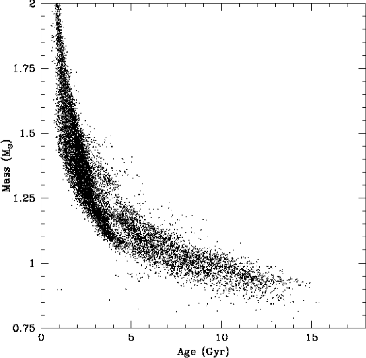
Figure 25: Age vs. mass for stars with well-defined ages. The apparent correlation of age and mass is an artifact caused by the over-representation of evolved stars and the fact that reliable ages cannot be determined for unevolved stars.

5.5 Completeness of ages

In Sect. 4.5.6 we discussed how we have determined errors for the ages derived for the individual stars. The degree of completeness of the age data depends, then, on how large errors one is willing to accept. For the total sample, publishable ages as defined in Sect. 4.5.6 are available for 13,636 stars or 82% of the full sample (9,158 or 83% of the single stars), of which 11,445 (and 7,566 single stars – 69% of the total in both cases) have “well-defined” ages by the definition in Sect. 4.5.6. If the relative error limits are set to 50% or 25%, the numbers are 9,428 and 5,472 (57% and 33%), respectively, for all stars, and 6,144 and 3,528 (or 56% and 32%) for the single stars.

The fraction of stars for which reliable ages can be derived varies strongly over the HR diagram. For the evolved F stars the situation is relatively favourable. For stars on or near the ZAMS, only an upper limit to the age can, in effect, be determined. And for the still-unevolved low-mass stars no usable ages can be determined at all; in our sample, essentially no star below 0.90 $M_{\odot}$ or fainter than $M_{V}=4.5$ yields a meaningful age.

These effects are evident in Fig. 25, which shows the correlation between the ages and masses derived for the stars in the sample. Three effects are obvious from the figure: (i): The upper envelope of masses for a given age, set by the evolution of the stars onto the giant branch (but blurred by metallicity effects); (ii): the lack of stars younger than $\sim 1$ Gyr, a direct result of our blue colour cut-off at b-y = 0.205; and (iii): the lack, at each age, of the low-mass, unevolved stars for which well-defined ages cannot be determined. The few scattered stars below the main relation are probably undetected giants or other peculiar stars.

6 Discussion

The data base presented here provides a basis for a thorough re-evaluation of some of the global properties of the Solar neighbourhood and the Galactic disk. Several of these analyses will require detailed simulations of the predictions of various competing models, subjecting the simulated stellar populations to the same selection criteria as used to establish our samples, and comparing the results with the real data set.

Such simulations will be the subject of future papers, but are beyond the scope of the present discussion. Here, we will simply review a few of the ’classic’ diagnostic relations for the Galactic disk, i.e, the metallicity distribution for long-lived stars, the age-metallicity relation for the Solar neighbourhood, the radial metallicity gradient, and the age-velocity and metallicity-velocity relations.

In each case, two features are essential: (i) the lack of kinematic selection bias in our sample; and (ii) the new radial-velocity data which allow to identify stars that have not taken part in the evolution of the local disk, but just happen to pass through it at this time; remove contamination by unrecognised binary stars; complete the velocity information for the sample, and estimate scale-height corrections. At the same time, the very strong absolute-magnitude bias in our sample and limitation of the coolest stars to the cap south of $-26\degr$ declination must be kept firmly in mind and corrected for as appropriate.

As a preliminary, we warn that the true uncertainty of the ages of especially the oldest stars must be kept in mind when interpreting the following diagrams (note in this connection that the final refinements in our age computation methods have resulted in significant changes in the ages of the oldest stars since our preliminary discussion in Holmberg et al. holmbetal03 (2003)).

As shown in Fig. 17, restricting the sample to stars with increasingly better-determined ages preferentially eliminates the oldest stars and makes it increasingly difficult to determine the maximum age of stars in the disk. Conclusions based on single points in, e.g. Figs. 27 or 30, will be risky at best. E.g., we note that the statement by Sandage et al. (sandage03 (2003)), that “the age of the field stars in the solar neighbourhood is found to be $7.9\pm 0.7$ Gyr”, is based on a few stars assumed (but not known) to be super-metal-rich and ignores the existence of binary stars on the main sequence. At the same time, the authors recognise that the open cluster NGC 6791, with [Fe/H] = +0.3-0.4, is about 10 Gyr old, a warning against quick conclusions drawn from a single diagram.

6.1 Metallicity distribution (the “G dwarf problem”)

Relative to the predictions of a closed-box model with constant initial mass function (see e.g. Pagel pagel97 (1997)), the observed metallicity distribution function for unevolved low-mass dwarfs shows a significant lack of low-mass metal-poor stars (van den Bergh vdbergh62 (1962), Schmidt schmidt63 (1963)). These should have been formed along with the high-mass stars that produced the heavy-element content of later stellar generations, but have not been found in the predicted numbers in previous surveys (“the G-dwarf problem”). While closed-box models are now obsolete, the metallicity distribution of long-lived stars remains a fundamental constraint on any of its successors.

The G-dwarf problem could in principle have two different explanations: (i): The ’missing’ metal-poor dwarfs do in fact exist, but have not been found by previous searches; a population of slow-moving metal-poor stars could exist which would be missed in proper-motion surveys, but be included in our sample. Or (ii): the Galactic disk did not evolve according to simple closed-box models.

The G-dwarf problem was rediscussed exhaustively by Jørgensen (bjarner00 (2000)), based on an early version of the present data set. We refer the interested reader to that paper for the full discussion, since no material changes have been made to the underlying data since that study.

Here we just recall the salient conclusion, i.e. that the solution to the G-dwarf problem is not a previously undiscovered metal-poor population. On the contrary, when drawn from a volume-complete and kinematically unbiased sample, the true fraction of metal-poor dwarfs is in fact only about half as large as previously believed, and the agreement with closed-box models even worse than before. Better physical models, not better data, are now the most urgent requirement. Fig. 26 shows the metallicity distribution for the volume complete part of our survey.

Figure 26: Distribution of metallicities for the volume complete sample of single stars (full histogram). For comparison the dotted curve shows the reconstructed distribution for G dwarfs from Jørgensen (bjarner00 (2000)), which is corrected for scale height effects and measurement errors.

6.2 Age-metallicity relations

Since the pioneering studies of Mayor (mayor74 (1974)) and Twarog (twarog80 (1980)), the relationship between average age and metallicity in the solar neighbourhood has been a subject of continuing debate, summarised in the recent study by Feltzing et al. (feltz01 (2001)). The debate concerns both the overall shape of the mean relation, whether there is scatter in the relation over and above that due to observational errors, and if so, what might be the cause of this scatter.

The accurate spectroscopic metallicities of Edvardsson et al. (edv93 (1993)) established beyond reasonable doubt that real scatter exists in the relation, far above that caused by observational errors. Little if any variation of mean metallicity with age was found, except for the very oldest stars ($>10$ Gyr) where a downturn was observed in agreement with previous studies. However, as pointed out by Edvardsson et al. (edv93 (1993)) themselves, the restriction of their sample to F-type dwarfs automatically excluded any old, metal-rich stars if such existed, a fact that has been overlooked in several later discussions. The very recent similar analysis by Reddy et al. (reddy03 (2003)) of a larger number of elements in 181 F and G dwarfs reached substantially the same conclusions as Edvardsson et al. (edv93 (1993)).

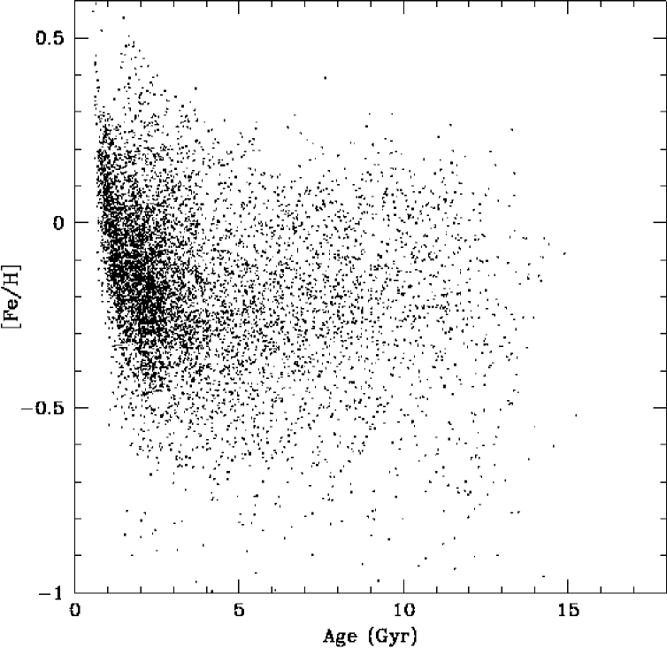
Figure 27: Age - metallicity diagram for 7,566 single stars with “well-defined” ages in the magnitude-limited sample. Note that individual age errors may still exceed 50% (cf. Fig. 16).

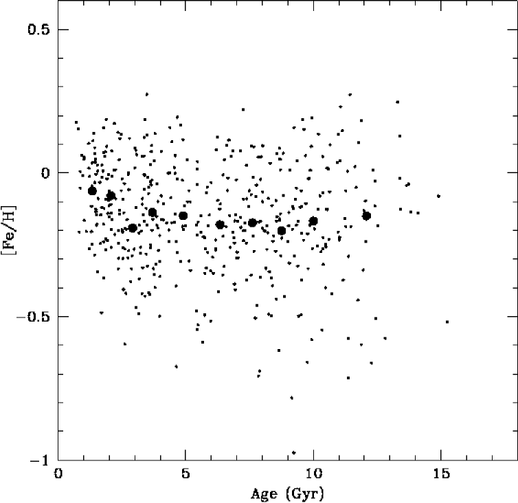
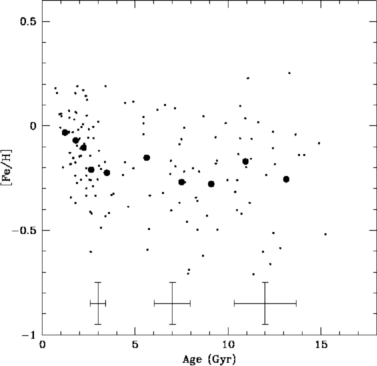
Figure 28: Age - metallicity diagrams for single stars in the volume-limited subsample within 40 pc; large dots show mean ages and metallicities in 10 bins with equal numbers of stars. Top: The 462 stars with “well-defined” ages (no limit on actual errors). bottom: The 142 stars with ages better than 25%; average error bars (14%) in three age bins are shown.

The selection criteria underlying the present sample were specifically designed to include the old, metal-rich stars that would have been missed by Edvardsson et al. (edv93 (1993)) even if they existed. At the same time, it was realised that these are just the stars for which the derived ages will be the most uncertain, as demonstrated implicitly by Feltzing et al. (feltz01 (2001)). In this context we note that Reddy et al. (reddy03 (2003)) find again a more clear-cut rise of mean metallicity with age than the two studies just mentioned, primarily because the Reddy et al. sample contains few old, metal rich stars. It is unclear whether this is caused by their selection procedure, and it is therefore of interest to re-examine the age-metallicity diagram constructed from the stars with well-defined ages in the unbiased sample presented here (see Figs. 27 and 28).

The most obvious features of Fig. 27 remain direct results of our selection criteria: The absence of stars near the lower left edge of the diagram is caused by our blue colour cutoff. The predominance of young, metal-rich stars is due to their intrinsic brightness and the correspondingly large volume they sample; the few young, apparently super-metal-rich stars are probably at least in part distant giant stars for which the interstellar reddening has been overestimated (see below and Burstein burst03 (2003)).

Apart from these features, little variation in mean metallicity is seen, except possibly for the very oldest stars which in general have kinematics characteristic of the thick disk. Even some of these have solar-like metallicities, however, and we note that Bensby et al. (bensby03 (2003)) recently derived a metallicity distribution for the thick disk that extends to stars with [Fe/H] $\geq 0$ and Sun-like [$\alpha$/Fe] abundance ratios; those stars are, however, also relatively young, so their thick-disk pedigree may remain open to question. The “$\zeta$ Herculis branch” of disk stars in the U-V diagram (Dehnen dehnen98 (1998), Skuljan et al. skuljan99 (1999)) could be a source of such stars.

When interpreting Fig. 27 (and Fig. 30), the substantial errors of even the “well-defined” ages should always be kept in mind; the presence of stars appearing to be as old as 14 Gyr is easily explained by observational errors. Uncertainties in the temperature scales of the observed stars and theoretical isochrones (Sect. 4.5.3) remain a potential source of systematic error, and numerical details of the age computation may introduce spurious features in diagrams such as Figs. 27 and 30, which can appear dramatic without the elaborate precautions described in Sect. 4.5.5, but may remain in more subtle form.

In order to avoid the strong absolute-magnitude bias in Fig. 27, we plot in Fig. 28 the same data for the volume-limited subsample within 40 pc. Despite the drastic reduction in number of stars, the lack of young metal-poor stars produced by our blue colour cutoff remains well visible and is responsible for the upturn of the mean relation for the youngest ages. The disappearance of the young “super-metal-rich” stars supports their interpretation as an artifact of the de-reddening procedure for distant giant stars. The lack of any overall metallicity variation in the thin disk is even more pronounced than before. Finally, the scatter in [Fe/H] at all ages again greatly exceeds the observational error of $\sim$0.1 dex. Limiting the sample to the best-determined ages leads to the same conclusions.

This picture of the age-metallicity distribution for field stars agrees well with the most recent studies of open clusters by Friel et al. (friel02 (2002)) and Chen et al. (chenl03 (2003)). These studies show the same constant mean metallicity and large scatter at all ages for the clusters as our study does for the field stars. The discussion by Sandage et al. (sandage03 (2003)) also focuses on the existence of old, metal-rich subgiants in their sample (the 10-Gyr-old metal-rich cluster NGC 6791 being another example) – as in fact pointed out already by Strömgren (stromgren63 (1963)). Clearly, more realistic models of the true complexities of star formation and chemical enrichment of the interstellar medium are required.

We recall that we have taken special pains to verify that our age computation technique will not distort the overall trends in the resulting age-metallicity diagrams (cf. Sect. 4.5.7). Individual ages shown in Figs. 27 and 28 (top) may still be uncertain by 50% or more, however (cf. Fig. 15), which must be taken into account in any discussion of these diagrams.

“Cleaner” subsamples of stars can be selected from the catalogue (e.g. Fig. 28, bottom), but introduce further strong selection effects; cf. the top and bottom panels of Figs. 28 and 30. Evaluating the true interplay of cosmic scatter in the chemical evolution of the disk with observational errors and uncertainties in the age determinations will require detailed numerical simulations, which must include models of the statistical biases discussed above and by Pont & Eyer (pont04 (2004)). Such detailed analyses are beyond the scope of the present paper.

6.3 Radial metallicity gradients in the disk

In addition to the evolution of metallicity with age, our sample can be used to study the radial metallicity gradient in the Galaxy. From the $R_{min}$ and $R_{max}$ of the stellar orbit, the mean orbital radius $R_{m}$ can be calculated. Fig. 29 shows the radial metallicity gradient for three groups of stars of different ages. The slopes of the fitted lines are -0.076$\pm$0.014, -0.099$\pm$0.011, and +0.028$\pm$0.036 dex/kpc.

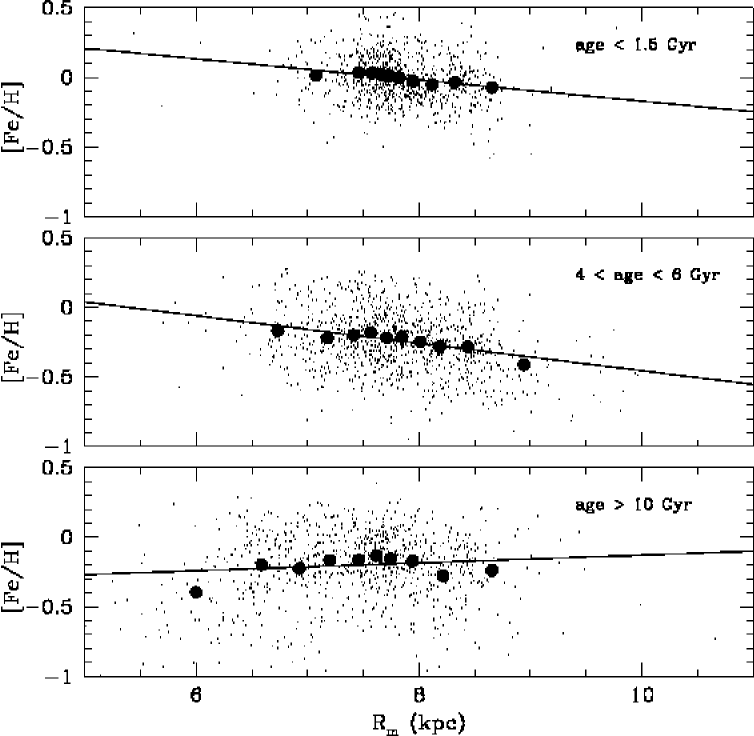
Figure 29: Radial metallicity gradient for single stars in three age ranges. $R_{m}$ is the mean radius of the stellar orbits.

This can be compared to other studies using FG dwarfs and giants by Mayor (mayor76 (1976)), Cepheids by Andrievsky et al. (andrievsky02 (2002)), planetary nebulae by Maciel et al. (maciel03 (2003)), and open clusters by Friel et al. (friel02 (2002)) and Chen et al. (chenl03 (2003)). In general they find the radial gradient to evolve over time from values between -0.02 and -0.06 for the youngest stars to between -0.08 and -0.12 for the older stars. This is compatible with our two younger age groups which show a mild steepening with age of the radial gradient. The oldest stars in our sample, on the other hand, show no radial gradient at all. This is an indication that these stars do not follow the general evolution of the younger stars in the disk, but are of a different origin, perhaps from the thick disk.

The radial metallicity gradient of $\sim$-0.09 dex/kpc seen for stars younger than 10 Gyr can be used in an attempt to correct the age-metallicity distribution for the effects of radial migration in the disk (cf. Wielen et al. wfd96 (1996)). This correction has no discernible effect on the distribution, and the dispersion around the mean for the volume-limited sample is unchanged: Computing the mean and standard deviation of the metallicities in the age range 2-12 Gyr in Fig. 28 (top), we find $<$[Fe/H]$>$ = -0.16, $\sigma$ = 0.20 dex with no correction, $<$[Fe/H]$>$ = -0.19, $\sigma$ = 0.20 dex after applying the correction for the radial metallicity gradient.

Stars migrating into the sample from orbits centered elsewhere in the disk obviously account for only a minute part of the scatter in the age-metallicity diagram, and both dispersions are clearly much larger than can be explained by errors in the metallicities, as also concluded by Edvardsson et al. (edv93 (1993)) and Reddy et al. (reddy03 (2003)) from detailed spectroscopy. Our removal of binaries from the sample and careful study of the age uncertainties also guarantee that poorly-determined ages do not affect this conclusion (and the main trends of Figs. 28 are insensitive to even substantial horizontal redistribution of the points in the range 2-12 Gyr).

6.4 Age-velocity relations

The observed space velocity components U, V, W for all single stars in the sample are shown as functions of age in Fig. 30, with weak as well as strong limits on the accuracy of the ages. The population of bright, early F-type stars is prominent, but otherwise the diagrams reflect the slow increase of the random velocities with age which is attributed to heating of the disk by massive objects such as spiral arms or giant molecular clouds. The rate of change and maximum velocity dispersion reached in the thin disk are of key importance for the interpretation in terms of the local dynamics of the disk itself.

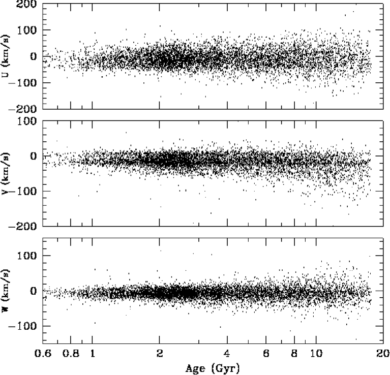
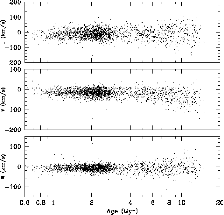
Figure 30: U, V and $W$ velocities as functions of age for all single stars with complete data. Top panels: All 7,237 stars with “well-defined” ages and all velocity data; bottom panels: The 2,852 stars with ages better than 25%.

Figure 31: Velocity dispersions for single stars with relative age errors $<$25% as functions of age (Fig. 30, bottom). From top to bottom, the total, U, V, and W velocity dispersion are plotted in 10 bins with equal numbers of stars. The lines show fitted power laws; see text for full details. The youngest and oldest age bins have been excluded from the fits to avoid biases due to unrelaxed young structures and thick disk stars, respectively.

In order to quantify these relations and also search for a kinematic signature of the thick disk, we have computed the velocity dispersions of the single stars with the best-determined ages. Fig. 31 shows the resulting relations and the power laws fitted to them, excluding the youngest and oldest bins. The resulting exponents are 0.31, 0.34, 0.47, and 0.34 for U, V, W, and the total velocity dispersion, respectively, with an uncertainty of 0.05, in close agreement with Holmberg (holmb01 (2001)) and Binney et al. (binney00 (2000)). Aside from the low exponent for the total velocity dispersion, the evolution of the velocities over time is characterised by a small increase in the ratio of $\sigma_{V}/\sigma_{U}$ and a larger increase in the ratio $\sigma_{W}/\sigma_{U}$. The consistency of these recent studies, which all use isochrone ages but otherwise different samples and methods, is in sharp contrast to studies using ages derived from chromospheric emission, which give values of either 0.26$\pm 0.01$ or 0.59$\pm 0.04$ (Hänninen & Flynn hanninen02 (2002)).

Fig. 30 shows no distinct jump in the velocity dispersion for the oldest stars as derived by Quillen & Garnett (qg01 (2001)) from the data by Edvardsson et al. (edv93 (1993)). Our result, derived from a sample $\sim 75$ times larger and with far more refined procedures for the age determination, should clearly be more reliable.

According to the classic Oort relation, $\sigma_{V}/\sigma_{U}$ should be constant and equal to 0.5 for a flat rotation curve (we find a value of $\sim 0.63$). Mühlbauer & Dehnen (muhlbauer03 (2003)) however, show that when the true velocity dispersion and non-axisymmetric disturbances of the disk are taken into account, large variations can occur. The smaller exponents for the in-disk heating ($\sigma_{U},\sigma_{V}$) compared to the out-of-the-disk heating ($\sigma_{W}$) gives further constraints to be fulfilled by models trying to explain the observed kinematic heating of the disk. At least four mechanisms have been proposed to explain the heating: fast perturbers from the halo, such as $10^{6}M_{\odot}$ black holes; slow perturbers in the disk, such as giant molecular clouds; large scale perturbations of the disk caused by spiral arms (De Simone et al. desimon04 (2004)) or the bar (e.g. Fux fux01 (2001)); and finally heating caused by infalling satellite galaxies.

Massive black holes are improbable candidates due to other observational constraints, apart from the fact that their heating index of 0.5 is too high. Infalling satellites should result in a single dramatic heating of the disk, such as the creation of the thick disk. Stable spiral arm patterns increase the random motions of stars within the plane but not perpendicular to it, and also become inefficient heaters when the epicyclic radius of a star gets larger than the length scale of the spiral pattern. Molecular clouds heat stars in all three directions, but in isolation they are inefficient heaters with a total exponent of only 0.21 and a vertical exponent of 0.26 in the simulations of Hänninen & Flynn (hanninen02 (2002)). Clearly, further simulations including realistic descriptions of all heating components are needed, and indeed the recent work on the effects of stochastic, transient spiral wave structures by De Simone et al. (desimon04 (2004)) is able to produce exponents in the observed range.

Wielen et al. (wfd96 (1996)) discussed the diffusion of stellar Galactic orbits as a possible explanation of the scatter from an otherwise single-valued age-metallicity relation, combined with a radial metallicity gradient in the disk. From our redetermination of the age-velocity relations based on a much larger sample and better data than available to them, we find a true dispersion of velocities and orbits which is insufficient to support that interpretation (see also Nordström et al. paris99 (1999)). One might suspect the velocity data used by Wielen et al. (wfd96 (1996)) to be contaminated by thick-disk or halo stars, or by undetected binary orbital motion.

Finally, we note that the continued heating of the disk throughout its lifetime shown in Fig. 31 is inconsistent with the results of Quillen & Garnett (qg01 (2001)) who found the heating of the thin disk to saturate after $\sim 2$ Gyr, with an abrupt increase in velocity dispersion when the thick disk appeared at $\sim 10$ Gyr. Presumably, this is due to their much smaller sample of stars (from Edvardsson et al. edv93 (1993)) and consequently larger statistical errors than ours, as well as possible temperature or colour shifts of the evolution models used to determine ages for cool dwarfs (see discussion in Sect. 4.5.1).

Fig. 31 does show a modest increase in velocity dispersion for the oldest age bin, suggestive of the appearance of the thick disk. The key new result is, however, that the disk heating does not saturate at an early stage. Continued heating of the disk would appear to make it more difficult to trace old moving groups and other fossils of past merger events in the present Galactic disk (see Freeman & Bland-Hawthorn freeman02 (2002)).

6.5 Metallicity-velocity relations

Given the lack of correlation between age and metallicity demonstrated in Sect. 6.2, plots of space motions vs. metallicity are not merely trivial transformations of the age-velocity relations in Sect. 6.4, but convey independent information.

Fig. 32 shows these diagrams, which display the expected similarity with both Figs. 20 and 30 but reveal new, significant features. The [Fe/H] - $V$ and [Fe/H] - $U$ diagrams are especially interesting, as they show that the structures seen in Fig. 20 cover a wide range in [Fe/H] as well as in age (Fig. 30). This is quite unlike the behaviour expected for stars in classical moving groups, which are presumed to have been born together, but resembles the kinematic structures produced by an inhomogeneous Galactic potential, e.g. by stochastic spiral waves (De Simone et al. desimon04 (2004)) or the bar (e.g. Fux fux01 (2001)).

In particular, the group of stars near $V=-50$ km s^-1 and $U=-50$ km s^-1 and with [Fe/H] between $\sim-0.7$ and $\sim+0.2$ suggest the existence of a population of kinematically focused stars with a range of thin-disk metallicities in addition to the bona fide thick-disk stars. This possibility is of interest in studies of the detailed characteristics of kinematically defined samples of thick-disk and thin-disk stars (see Bensby et al. bensby03 (2003) for a recent example).

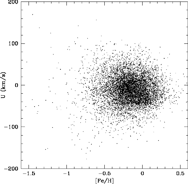
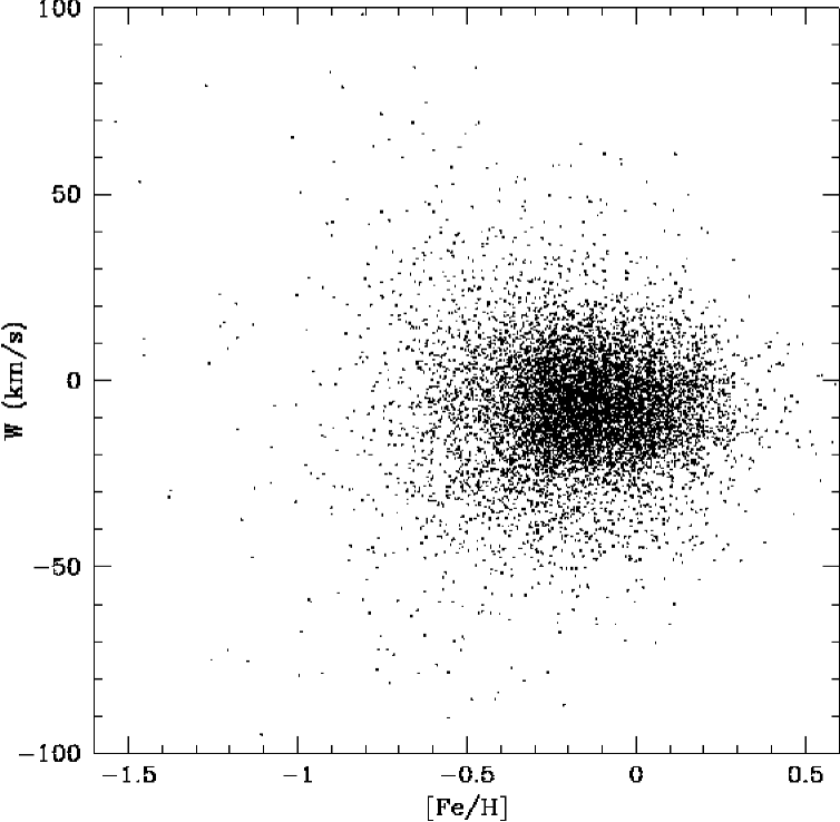
Figure 32: U, V, and W as functions of metallicity for all single stars in the sample.

7 Conclusions and outlook

The results presented here are the culmination of many years of effort by many people. Indeed, this is in essence the project for which not only the Strömgren $uvby$ photometric system (Strömgren stromgren63 (1963)), but also the CORAVEL radial-velocity scanners (Mayor mayor85 (1985)) were developed (and an important part of the science case for the Hipparcos satellite). We trust that the material presented here will remain useful to workers in the field for years to come.

The properties of the data set and the results of our first analysis of it are described in detail above; these descriptions will not be repeated here. Instead, it is interesting to reflect on the change of scene in Galactic research that has taken place in the three decades since the inception of this project (cf. the recent review by Freeman & Bland-Hawthorn freeman02 (2002), “The New Galaxy”).

At the time, the fundamental diagnostics of the evolution of the Galactic disk were the relations discussed in Sect. 6, and deriving isochrone ages was considered a fairly straightforward matter. What was needed was a much larger and better-defined data base and an improvement in accuracy to remove what was considered to be merely(?) observational scatter in the relations.

Having completed the observational effort and the first analysis of the data, we find ourselves with much better techniques for determining isochrone ages, but also a rather more conservative view of their accuracy than before. Ironically, the similar improvements in observational accuracy (Edvardsson et al. edv93 (1993) being the standard example) have only underscored the disagreement of the mean relations with the predictions of simple Galactic evolution models and the significance of the scatter around the relations in terms of the real mechanisms of the evolution of the disk.

Our age-metallicity diagrams (Fig. 27-28) should lay to rest the discussion whether closed-box models or single-valued predictions are adequate representations of the evolution of the Galactic disk. Models that allow for the coexistence of metal-poor and metal-rich stars throughout most of the life of the thin disk will be needed for further progress. Similarly, our new age-velocity relations will place much stronger constraints on models of the dynamical heating of disk stars; few if any of the traditional candidate mechanisms seem able to match the data. The new results will also be of importance for assessing the survival rates of star clusters and merger remnants in the disk and perhaps allow to detect the dynamical effects of the bar of the Milky Way (Fux fux01 (2001)). Finally, a reanalysis of the “G-dwarf problem” from a much larger and more rigorously selected data base points to a similar conclusion: The Galaxy is a far more complicated and interesting subject than ever before. The present work should lay the foundation for learning more about it.

Looking ahead a decade from now, the ESA cornerstone mission GAIA (Perryman et al. gaia01 (2001)) will provide the next quantum leap in our knowledge of the Galaxy. Obtaining the complementary photometry and radial velocities needed to fully exploit the astrometric data from Hipparcos was left to such independent ground-based efforts as the present programme (see also Udry et al. udryetal97 (1997)). In contrast, GAIA will obtain these observations with the same satellite payload as the astrometric data, although with much larger radial-velocity errors than achieved here (cf. Fig. 3). The present material should remain useful until the results from GAIA appear, not only for studying our Galaxy, but also in the efforts to optimise the observing and data reduction strategies for GAIA and for such precursor programmes as the RAVE survey (Steinmetz steinmetz (2003)).

Table 1. Table 1 will only be available in electronic form at the CDS. The two first pages of the table, listing the first 100 stars, are given at the end of this paper as sample of its content and format.

Table 2. Table 2 contains the mass ratios determined for 511 double-lined binary systems; it will be available as for Table 1.

Description of the columns in the catalogue
(Table 1; in electronic form only)

Left-hand pages (Fields 1-26)
(1) HIP : Number in the Hipparcos catalogue (ESA hipp97 (1997)), when available.
(2) Name : Other designation (HD, BD, CD or CP number, in order of preference). A second number following a slash indicates that a double star with separate HD numbers has been observed together.
(3) Comp : If the star is a member of a multiple system, the component(s) included in the photometry are identified here.
(4) $f_{b}$ : This flag identifies confirmed and suspected binaries. The information can come from one or several sources such as photometry, radial velocity or astrometry.
(5) $f_{s}$ : This flag identifies stars in the additional sample of cool dwarfs south of declination $-26\degr$ (see sect. 2.2 and 5.2).
(6-7) RA & Dec : Equatorial coordinates of the star (J2000 equinox and epoch), from the Tycho-2 catalogue.
(8-9) $l,b$ : Galactic coordinates of the star.
(10) $V$ : Johnson $V$ magnitude from the published $uvby$ photometry.
(11) b-y : The b-y colour in the Strömgren $uvby$ system.
(12) $\beta$ : The $H_{\beta}$ index in the Strömgren system.
(13) E(b-y) : Colour excess, from the calibrations of Olsen (eho88 (1988)).
(14) log$T_{eff}$ : Logarithm of the effective temperature, from the $uvby$ indices and the calibration by Alonso et al. (alonso96 (1996)).
(15) [Fe/H] : Metallicity of the star as determined from the $uvby\beta$ indices and the calibrations by Schuster & Nissen (schuni89 (1989)), Edvardsson et al. (edv93 (1993)) or the new calibration defined in Sect. 4.3.
(16) $d$ : Distance of the star, in parsecs (pc). Sect. 4.4 explains why some stars have no entry in this column.
(17) $M_{V}$ : Absolute magnitude, from the apparent magnitude, distance, and colour excess.
(18) $\delta M_{V}$ : The magnitude difference between the star and the ZAMS.
(19) $f_{r}$ : Source for the distance (see text). H = Hipparcos parallax; F,G = F or G-star photometric distance.
(20) $f_{g}$ : Suspected giant flag. An asterisk (*) indicates a disagreement between the photometric determination and the Hipparcos parallax at the $3\sigma$ level, suggesting that the star is a giant not detected from the photometry.
(21-23) age, $\sigma_{age}^{low}$, $\sigma_{age}^{high}$ : The age determined for the star, if any, with upper and lower $1\sigma$ confidence limits, all in Gigayears.
(24-26) mass, $\sigma_{mass}^{low}$, $\sigma_{mass}^{high}$ : The mass determined for the star, with upper and lower $1\sigma$ confidence limits, all in Solar masses.

Right-hand pages (Fields 27-51)
(27) Name : Repeated from field 2.
(28) $V_{r}$ : Mean radial velocity of the star. For double-lined binaries, the computed systemic velocity is given if so indicated by the flag $f_{d}$ in field 34.
(29) $m.e.$ : Mean error of the mean radial velocity. See text for details.
(30) $\sigma_{V_{r}}$ : Standard deviation of the individual radial-velocity measurements if $N>$ 1.
(31) $N$ : The number of individual radial-velocity measurements.
(32) $\Delta$T : Time-span, in days, from the first to the last radial-velocity observation.
(33) $P(\chi^{2})$ : Probability that the observed scatter of the radial velocities is due to random observational errors only.
(34) $f_{d}$ : This flag indicates that the star is a spectroscopic binary with a systemic radial velocity given in field 28.
(35) $f_{v}$ : Source of the radial velocity: C = Coravel; A = CfA; L = literature.
(36) $v$sin$i$ : Rotational velocity of the star, in km s^-1.
(37-39) $\mu_{\alpha*}$ $\mu_{\delta}$ $\sigma_{\mu}$ : Proper motion in right ascension and declination and standard error of the combined motion, in milliarcsec/year. Mostly from the Tycho-2 catalogue.
(40-41) $\pi$ $\sigma_{\pi}$ : Hipparcos parallax and its standard error, in milliarcsec.
(42-44) U V W : Heliocentric space velocity components for the star (U positive towards the Galactic centre), in km s^-1.
(45-46) $R_{gal}$, $z$ : Galactic position of the star, in kpc.
(47-50) $R_{min}$ $R_{max}$ $e$ $z_{max}$ : Perigalactic and apogalactic distance, eccentricity, and maximum distance from the galactic plane of the computed galactic orbit, in kpc.
(51) $f_{n}$ : General note (see below).
a: Double star with $\Delta m<$ 5 mag
b: Double star with $\Delta m<$ 5 mag from Hipparcos
c: Variable star
d: Simbad note
e: See Olsen (eho83 (1983))
f: See Olsen (eho79 (1979))
g: See Olsen (eho80 (1980))
h: See Olsen (eho93 (1993))
i: See Olsen (1994a )
j: See Olsen (1994b )
k: See Abt et al. (abt79 (1979))
l: See Abt (abt84 (1984))
m: See Abt (abt86 (1986))
n: See Gray & Garrison (graygar89 (1989))
o: See Gray (gray89 (1989))
p: See Henry et al. (henry96 (1996))

Table 2: Sample left-hand page of the catalogue (Fields 1-25 for the first 100 stars).

HIP	Name	Comp	$f_{b}$	$f_{s}$	RA J2000	Dec J2000	l	b	$V$	b-y	$\beta$	E(b-y)	$logT_{e}$	[Fe/H]	d	$M_{v}$	$\delta M_{v}$	$f_{r}$	$f_{g}$	age	$\sigma_{age}^{low}$	$\sigma_{age}^{high}$	mass	$\sigma_{mass}^{low}$	$\sigma_{mass}^{high}$
					h   m     s	o     ′    ′′	o	o	mag	mag		mag			pc	mag	mag			Gy	Gy	Gy	$M_{\odot}$	$M_{\odot}$	$M_{\odot}$
1	2	3	4	5	6	7	8	9	10	11	12	13	14	15	16	17	18	19	20	21	22	23	24	25	26
437	HD 15		*		00 05 17.8	+48 28 37	115	-14	8.304	0.592								G	*
431	HD 16				00 05 12.4	+36 18 13	113	-26	8.092	0.311			3.810	0.10
420	HD 23				00 05 07.4	-52 09 06	319	-64	7.552	0.366	2.626	0.015	3.770	-0.19	42	4.44	0.49	H		7.6	3.6	10.9	0.99	0.94	1.06
425	HD 24		*		00 05 09.7	-62 50 42	312	-53	8.146	0.377	2.607	0.013	3.763	-0.31	70	3.91	1.29	H		9.3	7.8	11.0	1.01	0.97	1.04
	HD 25				00 05 22.3	+49 46 11	115	-12	7.590	0.256	2.675	-0.005	3.828	-0.38	87	2.89	0.91	F		2.0	1.6	2.4	1.31	1.24	1.39
447	HD 26		*		00 05 22.2	+08 47 16	104	-52	8.238	0.645	2.546							G	*
461	HD 39	AB	*		00 05 29.0	+34 06 20	112	-28	7.852	0.337	2.628	0.014	3.784	-0.55	91	3.06	1.85	H		4.7	4.0	5.6	1.14	1.09	1.20
	HD 59				00 05 33.5	+46 39 46	115	-15	8.595	0.363	2.613	0.007	3.772	-0.24	87	3.90	1.03	F		7.4	5.3	9.8	1.02	0.97	1.09
462	HD 63		*		00 05 31.1	-09 37 02	89	-69	7.132	0.298	2.663	0.008	3.806	-0.20	51	3.62	0.50	H		2.9	1.7	3.8	1.21	1.15	1.26
459	HD 67			*	00 05 28.4	-61 13 33	313	-55	8.822	0.424			3.743	-0.14	54	5.17	0.33	H					0.87	0.83	0.96
475	HD 70				00 05 41.6	+58 18 47	117	-4	8.221	0.395	2.582	0.010	3.752	-0.49	48	4.83	0.74	H		14.9	7.4		0.84	0.81	0.90
482	HD 85	AB	*		00 05 44.4	+17 50 25	108	-44	7.754	0.275	2.661	-0.014	3.820	-0.08	87	3.06	0.64	F		1.9	1.3	2.3	1.35	1.28	1.43
493	HD 101				00 05 54.7	+18 14 06	108	-43	7.456	0.373	2.598	0.001	3.765	-0.32	38	4.55	0.61	H		9.4	5.4	14.2	0.94	0.87	1.00
490	HD 105				00 05 52.5	-41 45 11	333	-73	7.509	0.373	2.627	0.019	3.766	-0.21	40	4.49	0.55	H		8.6	4.8	12.6	0.97	0.92	1.03
	HD 117	ABC	*		00 05 57.0	-30 19 41	12	-80	9.047	0.385	2.644	0.077	3.800	-0.26	98	3.76	0.55	F		3.3	2.0	4.7	1.14	1.07	1.21
518	HD 123	AB	*		00 06 15.8	+58 26 12	117	-4	5.978	0.421			3.746	0.04	20	4.44	0.85	H		12.8	8.5	15.1	0.98	0.92	1.02
510	HD 126		*		00 06 08.0	+09 42 53	105	-52	7.803	0.312	2.647	0.002	3.798	-0.21	90	3.03	1.28	H		2.7	2.3	3.1	1.31	1.23	1.38
522	HD 142	AB	*		00 06 19.1	-49 04 30	322	-66	5.710	0.330	2.640	0.006	3.791	-0.09	26	3.67	0.68	H		3.6	2.8	4.3	1.20	1.12	1.25
530	HD 153				00 06 26.0	+42 45 09	114	-19	8.357	0.388	2.601	0.010	3.763	-0.16	123	2.90	2.16	H		3.8	3.1	4.9	1.30	1.18	1.36
529	HD 156				00 06 24.9	-18 02 17	72	-76	7.311	0.248	2.699	0.007	3.844	0.23	131	1.72	1.27	F		1.1	0.9	1.3	1.87	1.75	2.01
519	HD 160	AB	*		00 06 16.8	-64 14 25	311	-52	7.801	0.291	2.689	0.036	3.840	0.25	160	1.63	1.41	F		1.1	0.8	1.3	1.92	1.79	2.04
544	HD 166	A			00 06 36.7	+29 01 17	111	-33	6.093	0.460	2.576		3.727	-0.07	14	5.41	0.36	H		16.6	3.0		0.85	0.83	0.91
547	HD 189				00 06 39.5	-24 37 15	44	-80	8.560	0.347	2.633	0.018	3.783	-0.25	129	3.01	1.67	F		4.3	2.8	5.4	1.17	1.12	1.29
556	HD 200				00 06 46.9	-04 21 00	96	-65	8.222	0.357	2.605	0.000	3.774	-0.45	110	3.02	2.04	H		4.9	3.7	6.2	1.14	1.06	1.22
560	HD 203				00 06 50.0	-23 06 27	52	-79	6.190	0.256	2.689	0.003	3.830	-0.15	39	3.23	0.32	H		1.5	0.5	2.2	1.34	1.29	1.40
597	HD 219				00 07 13.7	+73 12 37	120	11	7.875	0.257			3.835	-0.17
	HD 220				00 07 04.7	+67 16 27	119	5	8.686	0.320	2.639	0.027	3.806	-0.58	133	2.95	1.49	F		2.8	2.3	4.5	1.18	1.11	1.29
578	HD 222				00 07 02.0	+22 50 40	110	-39	8.290	0.241	2.692	-0.007	3.840	-0.08	119	2.91	0.39	H		1.3	0.6	1.7	1.43	1.37	1.50
584	HD 233		*		00 07 07.6	-15 51 00	78	-75	8.680	0.331	2.638	0.018	3.787	-0.44	86	4.01	0.74	F		5.2	2.5	7.6	1.04	0.97	1.10
603	HD 251		*		00 07 18.3	+07 42 12	104	-54	7.637	0.309	2.636	-0.004	3.802	-0.32	108	2.47	1.84	F		2.2	1.9	2.6	1.42	1.32	1.51
606	HD 268				00 07 22.5	-25 21 23	41	-80	7.064	0.306	2.643	0.003	3.800	-0.37	49	3.63	0.77	H		3.5	2.7	4.3	1.15	1.08	1.20
596	HD 276				00 07 13.4	-76 43 51	306	-40	7.556	0.271	2.677	0.006	3.821	-0.29	84	2.93	0.93	H		2.2	1.9	2.5	1.35	1.30	1.40
612	HD 285				00 07 28.1	-56 00 41	315	-60	7.489	0.297	2.649	0.002	3.809	-0.29	133	1.86	2.27	H		1.6	1.4	1.8	1.61	1.53	1.71
630	HD 291				00 07 40.4	+39 02 05	114	-23	8.019	0.297	2.660	0.009	3.808	-0.24	104	2.93	1.18	H		2.4	2.1	2.8	1.33	1.26	1.40
634	HD 292	AB	*		00 07 43.1	+37 11 07	113	-25	7.436	0.317			3.800	-0.12	139	1.72	2.46	H		1.5	1.3	1.8	1.70	1.57	1.81
641	HD 299				00 07 52.0	+55 34 37	117	-7	7.831	0.388			3.762	-0.04	46	4.52	0.46	H		8.1	3.6	11.8	0.99	0.94	1.06
624	HD 307				00 07 37.4	-45 07 10	326	-70	8.198	0.379	2.609	0.015	3.768	-0.17	122	2.77	2.19	H		3.6	2.8	4.5	1.32	1.25	1.39
	HD 308			*	00 07 37.8	-51 57 17	318	-64	9.402	0.438			3.737	-0.24	78	4.94	0.76	G			11.7		0.86	0.83	0.91
618	HD 309	AB	*		00 07 34.7	-60 38 30	312	-56	8.379	0.382	2.621	0.030	3.781	-0.04	87	3.55	0.99	F		3.6	2.7	5.9	1.15	1.09	1.25
656	HD 330				00 08 04.6	+53 47 46	116	-9	8.151	0.384	2.597	0.005	3.762	-0.39	102	3.11	2.18	H		5.1	3.9	6.5	1.12	1.05	1.24
650	HD 333				00 08 00.7	+29 50 15	112	-32	7.538	0.261	2.697	0.022	3.849	0.13	189	1.06	1.93	F		0.8	0.7	0.9	2.09	1.97	2.26
649	HD 334				00 08 00.2	-07 32 40	93	-68	7.848	0.317	2.638	0.004	3.797	-0.27	93	2.99	1.39	H		2.7	2.3	4.2	1.30	1.18	1.38
669	HD 361				00 08 16.3	-14 49 28	82	-74	7.045	0.388	2.598	0.004	3.758	-0.20	28	4.84	0.38	H		9.2	0.7	16.1	0.92	0.85	1.01
697	HD 372		*		00 08 35.3	+53 15 14	116	-9	7.752	0.281			3.817	-0.24	114	2.47	1.44	H		1.9	1.7	2.2	1.46	1.38	1.55
691	HD 373				00 08 30.1	+52 20 11	116	-10	7.782	0.241	2.688	-0.004	3.835	-0.40	69	3.57	0.11	H				1.8	1.24	1.19	1.29
689	HD 375				00 08 28.4	+34 56 04	113	-27	7.409	0.377			3.771	0.05	79	2.93	1.77	H		2.7	2.4	4.0	1.44	1.33	1.49
682	HD 377				00 08 25.7	+06 37 00	104	-55	7.581	0.391	2.603	0.001	3.760	-0.02	40	4.58	0.43	H		8.2	3.4	12.2	0.99	0.93	1.06
	HD 382				00 08 25.4	-21 24 31	61	-79	8.346	0.512			3.702	-0.42	27	6.19	0.31	G					0.75	0.72	0.79
688	HD 392				00 08 27.6	-24 05 37	48	-80	7.599	0.321	2.643	0.008	3.799	-0.12	132	2.00	2.20	H		1.7	1.4	2.0	1.61	1.52	1.71
699	HD 400				00 08 40.9	+36 37 37	113	-25	6.190	0.332	2.615	-0.011	3.787	-0.35	33	3.60	1.08	H		6.1	3.4	7.1	1.09	1.04	1.15
723	HD 404	A			00 08 57.2	+66 27 23	119	4	8.622	0.516			3.708	0.31	32	6.10	-0.14	H					0.88	0.83	0.90
	HD 410			*	00 08 35.1	-66 25 01	310	-50	9.425	0.426			3.745	0.06	90	4.65	0.64	G		11.2	6.3	15.6	0.95	0.89	1.02
706	HD 427				00 08 46.1	-34 47 39	350	-78	7.882	0.299	2.636	-0.016	3.808	-0.12	111	2.66	1.34	F		2.1	1.8	2.5	1.42	1.34	1.51
746	HD 432	A			00 09 10.6	+59 08 59	118	-3	2.270	0.216	2.709	-0.005	3.862	0.18	17	1.16	1.60	H		0.7	0.6	0.8	2.09	2.07	2.24
722	HD 435				00 08 56.5	+12 48 15	107	-49	8.477	0.353	2.637	0.017	3.779	-0.11	78	4.03	0.62	H		5.2	2.9	7.7	1.08	1.02	1.15
709	HD 439				00 08 48.4	-47 03 38	323	-68	7.817	0.304	2.670	0.020	3.820	0.13	116	2.40	1.11	H		1.5	1.2	1.7	1.60	1.52	1.70
740	HD 447				00 09 04.3	+19 55 28	110	-42	7.114	0.301	2.645	-0.006	3.810	-0.08	115	1.81	2.11	H		1.4	1.2	1.6	1.74	1.65	1.82
726	HD 457				00 08 59.6	-39 44 13	335	-75	7.725	0.391	2.617	0.018	3.765	0.11	55	4.03	0.76	H		6.6	3.6	8.7	1.12	1.06	1.19
747	HD 460	A	*		00 09 10.2	+44 43 18	115	-18	8.782	0.306	2.640	0.001	3.800	-0.44	129	3.23	1.23	F		3.1	2.5	5.0	1.16	1.09	1.24
732	HD 466				00 09 02.6	-35 05 30	349	-78	7.779	0.268	2.686	0.012	3.827	-0.05	154	1.84	1.68	H		1.3	1.1	1.5	1.71	1.60	1.82
730	HD 469	AB	*		00 09 02.3	-54 00 06	316	-62	6.332	0.460					143	0.56		H
754	HD 471	A	*		00 09 15.7	+25 16 55	111	-37	7.789	0.421	2.590		3.745	-0.16	45	4.51	0.96	H		14.4	10.6		0.90	0.86	0.96
759	HD 483		*		00 09 19.4	+17 32 02	109	-44	7.065	0.404	2.601	0.009	3.756	0.04	52	3.49	1.57	H		5.6	5.0	6.4	1.18	1.14	1.22
768	HD 489	AB	*		00 09 28.1	+19 06 56	109	-43	7.953	0.421	2.591		3.747	0.01	72	3.65	1.64	H		7.3	5.7	9.0	1.11	1.04	1.18
761	HD 493	AB	*		00 09 21.0	-27 59 16	25	-81	5.420	0.273	2.668	-0.003	3.826	-0.05	68	1.24	2.30	H		1.0	0.9	1.1	1.97	1.87	2.03
762	HD 494		*	*	00 09 23.3	-41 02 40	332	-74	9.118	0.492			3.715	0.08	84	4.50	1.42	H		17.3	13.2		0.93	0.90	1.00
795	HD 531	AB	*		00 09 51.2	+08 27 11	106	-53	8.650	0.439	2.583		3.737	-0.04	53	5.03	0.51	G		15.6	4.6		0.89	0.85	0.95
786	HD 536	AB	*		00 09 41.5	-37 18 53	341	-77	8.355	0.287	2.669	0.008	3.814	-0.17	123	2.91	1.00	F		2.2	1.8	2.6	1.34	1.26	1.43
794	HD 546	AB	*	*	00 09 50.0	-33 47 20	354	-79	8.832	0.498			3.709	-0.11	58	5.00	1.16	H
791	HD 547				00 09 48.5	-40 53 34	332	-74	8.578	0.408	2.590	0.013	3.750	-0.34	72	4.29	1.22	H		13.8	11.0	16.7	0.91	0.85	0.96
801	HD 564				00 09 52.8	-50 16 04	319	-66	8.323	0.381	2.584	-0.005	3.761	-0.33	53	4.69	0.57	H		10.6	4.5	16.0	0.91	0.84	0.99
	HD 570	AB	*		00 10 24.7	+58 31 25	118	-4	8.217	0.207			3.868	0.26
815	HD 578				00 10 02.5	-63 17 48	311	-53	8.134	0.290	2.661	0.001	3.812	-0.19	104	3.05	0.92	H		2.4	1.9	2.8	1.33	1.26	1.39
848	HD 583		*		00 10 24.0	+58 29 22	118	-4	7.738	0.297			3.807	-0.32	96	2.82	1.38	H		2.4	2.1	2.7	1.35	1.28	1.41
851	HD 604				00 10 26.3	-14 27 08	84	-74	8.353	0.331	2.610	-0.029	3.790	-0.24	131	2.77	1.75	F		2.7	2.2	4.1	1.34	1.19	1.45
819	HD 610				00 10 04.4	-79 00 06	305	-38	7.878	0.294	2.663	0.006	3.810	-0.17	90	3.10	0.90	H		2.4	2.0	2.8	1.33	1.27	1.38
856	HD 615				00 10 29.5	+15 13 54	109	-46	8.245	0.306	2.650	-0.004	3.804	-0.02	78	3.80	0.19	H		1.9		3.4	1.22	1.16	1.28
867	HD 631				00 10 39.1	+12 49 12	108	-49	8.475	0.366	2.611	0.003	3.771	-0.18	64	4.44	0.46	H		7.1	2.6	10.6	1.00	0.95	1.07
870	HD 633				00 10 40.7	+02 03 19	103	-59	7.514	0.313	2.643	-0.004	3.799	-0.08	55	3.81	0.35	H		2.9	0.8	4.2	1.19	1.14	1.25
880	HD 639		*		00 10 46.8	+37 28 26	114	-25	7.764	0.272			3.824	-0.16	114	2.49	1.19	H		1.8	1.5	2.0	1.49	1.42	1.57
889	HD 652	A			00 10 56.0	+48 06 37	116	-14	8.429	0.354	2.621	0.004	3.777	-0.16	61	4.52	0.22	H		4.0		8.8	1.03	0.96	1.09
872	HD 659		*		00 10 42.4	-54 24 01	315	-62	8.548	0.456			3.728	-0.25				G	*
865	HD 661/2		*		00 10 38.5	-73 13 27	307	-44	6.657	0.233	2.719	0.014	3.849	0.20	66	2.55	0.38	H		0.9	0.6	1.3	1.67	1.60	1.72
910	HD 693				00 11 15.8	-15 28 04	82	-75	4.910	0.326	2.617	-0.008	3.789	-0.49	19	3.53	1.22	H		5.7	4.8	6.9	1.07	1.03	1.14
	HD 694				00 11 18.0	-21 14 58	64	-79	8.339	0.341	2.644	0.018	3.786	-0.12	84	3.72	0.78	F		3.7	2.7	5.9	1.13	1.06	1.20
920	HD 700				00 11 24.4	+23 49 05	111	-38	8.239	0.362	2.621	0.011	3.771	-0.25	54	4.59	0.37	H		7.3	0.3	11.6	0.97	0.91	1.05
914	HD 705		*	*	00 11 18.0	-32 48 01	357	-80	8.601	0.430			3.738	-0.25	66	4.50	1.19	H		17.5	14.2		0.88	0.86	0.92
931	HD 717	AB	*		00 11 35.2	-03 04 40	100	-64	7.580	0.345	2.638	0.018	3.783	-0.21	66	3.48	1.17	F		5.2	3.1	6.7	1.12	1.06	1.20
937	HD 732				00 11 36.4	-23 37 56	52	-80	7.945	0.355	2.639	0.022	3.796	0.20	107	2.70	1.28	F		2.2	1.8	2.7	1.49	1.40	1.59
924	HD 734	A		*	00 11 30.8	-49 37 45	319	-66	9.143	0.448			3.728	-0.33	48	5.74	0.20	H					0.81	0.77	0.86
924	HD 734	B	*	*	00 11 30.2	-49 37 41	319	-66	10.987	0.655					48	7.59		H
952	HD 737		*		00 11 45.7	+27 30 36	112	-35	8.449	0.303	2.642	-0.004	3.804	-0.25	92	3.64	0.57	H		3.1	2.0	4.1	1.17	1.10	1.24
947	HD 738		*		00 11 40.8	-09 42 10	93	-70	8.530	0.324	2.645	0.014	3.794	-0.24	129	2.98	1.44	F		2.8	2.3	4.4	1.27	1.13	1.38
950	HD 739				00 11 44.0	-35 07 59	347	-78	5.250	0.290	2.653	-0.010	3.811	-0.13	22	3.55	0.39	H		2.4	1.0	3.2	1.25	1.21	1.30
929	HD 741			*	00 11 33.0	-58 54 35	312	-57	8.355	0.398			3.755	-0.26	59	4.51	0.83	H		13.2	8.8		0.91	0.85	0.97
956	HD 744	AB	*		00 11 50.1	+28 25 24	112	-34	7.510	0.322	2.622	-0.008	3.791	-0.45	78	3.05	1.62	H		4.4	2.9	5.3	1.16	1.10	1.25
944	HD 749		*		00 11 38.0	-49 39 21	319	-66	7.903	0.672								G	*
934	HD 750			*	00 11 35.7	-57 28 21	313	-59	9.013	0.492			3.707	-0.35	36	6.21	0.15	H					0.76	0.73	0.81
971	HD 755		*		00 12 01.4	+28 36 23	113	-33	7.194	0.253	2.690	0.006	3.836	-0.08	92	2.38	0.99	H		1.4	1.2	1.7	1.56	1.50	1.63
964	HD 768				00 11 54.7	-22 49 03	56	-80	7.934	0.238	2.696	-0.004	3.840	-0.15	92	3.12	0.24	H		1.2		1.8	1.37	1.32	1.44

Table 2: Sample right-hand page of the catalogue (Fields 26-50 for the first 100 stars).

Name	$V_{r}$	m.e	$\sigma_{V_{r}}$	N	$\Delta T$	$P(\chi^{2})$	$f_{d}$	$f_{v}$	$v$sin$i$	$\mu_{\alpha*}$	$\mu_{\delta}$	$\sigma_{\mu}$	$\pi$	$\sigma_{\pi}$	U	V	W	$R_{gal}$	$z$	$R_{min}$	$R_{max}$	$e$	$z_{max}$	$f_{n}$
	km/s	km/s	km/s		d				km/s		mas/yr		mas	mas	km/s	km/s	km/s	kpc	kpc	kpc	kpc		kpc
27	28	29	30	31	32	33	34	35	36	37	38	39	40	41	42	43	44	45	46	47	48	49	50	51
HD 15	-22.6	2.4	3.4	2	381	0.000		C	2	-4	-10	2	3.2	1.0										a
HD 16	-10.7	1.7	1.4	2	1848	0.556		C		28	-7	2	2.5	0.9
HD 23	34.3	0.2	0.3	3	1767	0.309		C	4	-111	-131	2	23.9	0.9	40	-22	-16	7.986	-0.037	6.39	8.88	0.16	0.15
HD 24	-26.9	0.2	19.0	5	1806	0.000	*	C	9	64	20	2	14.2	0.8	-31	7	15	7.972	-0.057	7.74	9.09	0.08	0.38	a
HD 25	-2.2	1.5						L		-30	-68	2			19	1	-24	8.036	-0.019	7.54	9.03	0.09	0.28
HD 26	-215.1	0.2	1.6	103	5879	0.000		C	5	261	-59	2	1.7	1.3										a
HD 39	-26.8	0.8	1.4	3	661	0.006		C	14	-18	26	2	11.0	0.9	11	-15	24	8.030	-0.042	7.24	8.37	0.07	0.55	a
HD 59	-34.2	0.3	0.2	2	94	0.626		C	4	159	40	2			-48	-57	13	8.035	-0.023	5.10	8.31	0.24	0.33
HD 63	0.2	2.1	3.0	2	1507	0.000		C	24	88	-72	1	19.8	0.9	-10	-24	-10	8.000	-0.047	6.91	8.00	0.07	0.06	a
HD 67	6.3	0.3	0.1	2	1085	0.986		C	4	84	-78	2	18.6	0.9	-10	-28	2	7.979	-0.044	6.65	7.98	0.09	0.14
HD 70	-28.4	0.2	0.4	3	727	0.287		C	3	65	-166	2	21.0	1.1	7	-31	-37	8.022	-0.003	6.49	8.13	0.11	0.52
HD 85	-12.0	2.4		1	0			C		60	-18	2	5.9	1.7	-16	-24	-1	8.019	-0.060	6.91	8.03	0.08	0.10	a
HD 101	-45.6	0.1	0.2	7	2452	0.924		C	2	-149	-151	1	26.2	0.8	46	-34	17	8.009	-0.026	5.86	8.84	0.20	0.41	b
HD 105	1.6	0.3	0.5	4	3363	0.176		C	15	98	-76	1	24.9	0.9	-10	-21	-2	7.989	-0.038	7.02	7.99	0.06	0.09	d
HD 117	15.0	0.3	0.2	3	361	0.842		C	11	-6	-10	3			7	-2	-14	7.983	-0.096	7.68	8.54	0.05	0.15	a
HD 123	-8.0	5.0	1.3	10	2676	0.000	*	C	5	271	30	2	49.3	1.0	-20	-19	-1	8.009	-0.001	7.13	8.07	0.06	0.09	a
HD 126	11.9	1.7	2.4	2	829	0.276		C		20	-13	2	11.1	1.0	-7	0	-14	8.014	-0.071	8.00	8.34	0.02	0.13	b
HD 142	5.3	0.3	0.1	2	1528	0.800		C	11	575	-37	1	39.0	0.6	-58	-37	-15	7.992	-0.023	5.82	8.58	0.19	0.12
HD 153	-31.8	0.3	0.2	2	133	0.645		C	5	78	-1	2	8.1	0.9	-27	-48	2	8.048	-0.041	5.61	8.12	0.18	0.14
HD 156	13.6	2.4						L		16	1	2	6.7	0.9	-8	-1	-15	7.990	-0.127	7.98	8.30	0.02	0.17
HD 160	17.2	1.8						L		28	23	2	5.4	1.7	-16	-4	-28	7.936	-0.126	7.82	8.16	0.02	0.35	a
HD 166	-6.9	0.1	0.3	21	5410	0.162		C	4	380	-178	1	73.0	0.8	-15	-22	-10	8.004	-0.007	7.01	8.02	0.07	0.04	c
HD 189	7.6	0.3	0.1	2	244	0.846		C	9	-25	-68	2	5.6	1.1	34	-28	-8	7.983	-0.127	6.21	8.61	0.16	0.13
HD 200	-0.2	0.2	0.2	2	360	0.635		C	5	59	-88	1	9.1	1.1	-4	-50	-23	8.005	-0.099	5.56	8.01	0.18	0.27
HD 203	6.5	3.5						L		97	-47	1	25.6	0.8	-11	-15	-10	7.995	-0.038	7.40	8.00	0.04	0.06	d
HD 219	-20.0	3.7						L		43	-11	2	4.2	0.7
HD 220										-32	14	2						8.064	0.011
HD 222										13	-16	1	8.4	0.9				8.031	-0.075					c
HD 233	-12.2	0.4	0.5	2	360	0.178		C	11	70	-23	2	7.9	2.3	-21	-24	5	7.995	-0.083	6.83	8.05	0.08	0.20	b
HD 251	17.2	1.1	1.9	3	365	0.364		C	45	-5	-6	2	5.9	1.7	1	9	-15	8.016	-0.087	7.95	9.05	0.07	0.16	b
HD 268	8.4	0.2	0.1	2	361	0.797		C	9	213	-133	2	20.6	0.9	-27	-48	-18	7.994	-0.048	5.58	8.06	0.18	0.17
HD 276	23.0	0.3	0.5	2	381	0.216		C	7	78	-5	2	11.9	0.6	-16	-30	-19	7.962	-0.054	6.55	7.98	0.10	0.18
HD 285	-0.9	0.5	0.6	2	358	0.151		C	13	74	24	2	7.5	0.8	-46	-9	-14	7.953	-0.116	7.05	8.78	0.11	0.16
HD 291	-17.6	0.3	0.1	2	363	0.946		C	6	-68	-58	1	9.6	0.9	45	-7	-13	8.039	-0.041	6.82	9.48	0.16	0.11
HD 292	0.7	0.3	0.2	2	363	0.664		C	10	11	-16	2	7.2	0.9	-3	-6	-11	8.050	-0.058	7.86	8.21	0.02	0.08	b
HD 299	1.4	0.2	0.2	3	1765	0.820		C	8	201	8	2	21.8	0.8	-39	-19	-6	8.021	-0.005	6.87	8.44	0.10	0.02	c
HD 307	14.6	0.2	0.2	4	1477	0.580		C	4	29	-98	2	8.2	1.0	12	-59	0	7.965	-0.115	5.03	8.06	0.23	0.16
HD 308	-33.4	0.3	0.1	2	360	0.870		C	1	114	38	2			-53	1	18	7.974	-0.070	7.24	9.41	0.13	0.47	d
HD 309	56.2	0.7	1.0	2	1215	0.007		C	7	34	-53	2	8.9	1.5	16	-46	-38	7.967	-0.072	5.67	8.13	0.18	0.56	a
HD 330	-42.5	0.3	0.6	3	714	0.076		C	4	73	-63	2	9.8	1.0	-5	-56	-29	8.045	-0.015	5.32	8.05	0.20	0.34
HD 333										1	6	2	3.8	0.9				8.059	-0.100
HD 334	-25.4	0.3	0.5	2	607	0.260		C	10	-29	29	2	10.7	1.0	6	6	30	8.002	-0.087	7.85	9.06	0.07	0.73
HD 361	7.7	0.2	0.4	6	3621	0.154		C	3	-14	-10	2	36.2	1.0	2	2	-7	7.999	-0.027	7.86	8.62	0.05	0.03
HD 372	-18.1	3.2	4.5	2	132	0.001		C	35	85	-3	1	8.8	0.9	-31	-37	-6	8.050	-0.018	6.12	8.19	0.14	0.02	a
HD 373	-6.2	0.6	0.8	3	1147	0.543		A	35	80	24	2	14.4	1.0	-22	-17	5	8.030	-0.012	7.24	8.13	0.06	0.17	g
HD 375	-5.7	0.2	0.1	2	363	0.815		C	5	114	10	2	12.7	0.9	-36	-23	-1	8.027	-0.036	6.74	8.34	0.11	0.10	b
HD 377	1.3	0.3	0.3	2	1437	0.475		C	13	85	-3	2	25.1	1.0	-14	-7	-4	8.006	-0.033	7.84	8.06	0.01	0.06	c
HD 382	1.2	0.2	0.2	2	1305	0.452		C	2	137	35	2			-17	-4	-4	7.997	-0.026	7.86	8.22	0.02	0.06
HD 392	-3.0	2.0						L		46	8	2	7.6	0.9	-28	-9	-2	7.984	-0.130	7.44	8.33	0.06	0.16
HD 400	-15.2	0.1	0.3	20	4858	0.831		C	6	-115	-124	2	30.3	0.7	28	-10	-8	8.012	-0.014	7.03	8.84	0.11	0.02
HD 404	-60.8	0.4		1	0			C	2	178	2	1	31.3	2.1	6	-66	-8	8.015	0.002	4.79	8.06	0.25	0.02	c
HD 410	-36.2	0.3	0.4	2	362	0.283		C	3	149	79	2			-80	13	-3	7.963	-0.069	6.96	10.81	0.22	0.12
HD 427	-20.9	0.6	1.0	3	1161	0.310		C	27	6	7	2	5.0	0.9	-8	2	20	7.977	-0.109	7.97	8.52	0.03	0.48
HD 432	12.6	1.6						L		523	-180	1	59.9	0.6	-39	-8	-22	8.008	-0.001	7.28	8.69	0.09	0.22	c
HD 435	8.7	0.3	0.2	2	1904	0.531		C	7	38	-38	2	12.9	1.0	-8	-10	-18	8.015	-0.058	7.74	8.03	0.02	0.16
HD 439	5.9	2.6	3.6	2	923	0.044		C	55	100	-45	1	8.6	0.9	-37	-48	-7	7.966	-0.108	5.52	8.13	0.19	0.11
HD 447	11.3	1.1	0.2	2	437	0.910		C	50	11	21	1	8.7	0.8	-13	11	0	8.029	-0.077	8.02	9.14	0.06	0.14
HD 457	-19.4	0.2	0.1	3	1477	0.856		C	3	112	-16	2	18.2	0.9	-28	-16	15	7.987	-0.053	7.20	8.21	0.07	0.36
HD 460	-13.9	0.6	1.2	4	439	0.016		C	6	53	-33	1	4.8	2.0	-17	-31	-20	8.052	-0.039	6.54	8.07	0.10	0.20
HD 466	-16.3	0.9	0.9	4	1116	0.758		A	60	37	-12	2	6.5	0.8	-23	-20	13	7.968	-0.150	7.05	8.06	0.07	0.36
HD 469	-1.1	0.2	0.2	2	1050	0.585		C	3	47	13	1	7.0	0.7	-31	-7	-8	7.952	-0.126	7.43	8.43	0.06	0.13	a
HD 471	5.0	10.9	15.5	2	793	0.000		C	1	173	-149	1	22.1	2.3	-21	-29	-34	8.013	-0.027	6.66	8.06	0.10	0.45	a
HD 483	-31.4	0.1	20.4	36	753	0.000	*	C	4	3	-131	1	19.3	0.8	21	-40	-1	8.012	-0.036	5.89	8.26	0.17	0.10	a
HD 489	-31.0	0.2	0.2	3	739	0.554		C	4	269	29	1	13.8	1.3	-77	-59	13	8.018	-0.049	4.80	8.81	0.30	0.35	a
HD 493	7.7	1.6						L		78	-16	6	14.6	1.3	-18	-16	-12	7.990	-0.068	7.30	8.05	0.05	0.09	a
HD 494	6.0	5.0	67.2	2	803	0.000	*	C	0	137	-137	2	11.9	1.3	-23	-74	-2	7.979	-0.081	4.43	8.01	0.29	0.11	a
HD 531	13.9	0.4		1	0			C	9	54	-10	3	14.2	4.2	-13	0	-15	8.009	-0.042	7.99	8.37	0.02	0.12	a
HD 536	-1.4	0.9	0.8	2	370	0.533		C	30	-53	-24	2	6.9	1.4	33	2	8	7.973	-0.120	7.24	9.42	0.13	0.28	a
HD 546	11.3	0.2	0.1	2	795	0.737		C	6	-62	-150	2	17.1	1.9	36	-29	-5	7.989	-0.057	6.18	8.65	0.17	0.07	a
HD 547	14.3	0.2	0.3	3	1476	0.340		C	3	138	-118	1	13.9	1.1	-20	-59	-13	7.982	-0.069	5.10	8.00	0.22	0.11
HD 564	11.1	0.2	0.3	5	3659	0.448		C	3	-96	-19	2	18.8	1.0	26	4	-4	7.983	-0.048	7.41	9.32	0.11	0.07
HD 570										-5	-9	2												a
HD 578	-2.9	0.4	0.1	2	769	0.906		C	14	-47	-39	2	9.6	0.8	25	-2	17	7.959	-0.083	7.28	9.01	0.11	0.43
HD 583	-20.1	1.4	1.9	2	132	0.001		C	13	-99	-10	2	10.4	0.8	49	3	4	8.044	-0.007	7.01	10.07	0.18	0.19	a
HD 604	3.5	0.5	0.6	2	607	0.201		C	10	69	-52	2	6.2	1.0	-21	-46	-18	7.996	-0.126	5.72	8.03	0.17	0.20
HD 610	11.2	0.4	0.6	2	312	0.188		C	14	13	-4	2	11.1	0.7	0	-11	-7	7.959	-0.055	7.49	8.09	0.04	0.06
HD 615	-4.6	0.4	0.1	3	1790	0.953		C	16	-70	-63	1	12.9	1.1	34	-5	-8	8.017	-0.056	7.09	9.20	0.13	0.06
HD 631	32.3	0.2	0.3	4	1162	0.618		C	6	38	-17	1	15.6	1.2	-14	12	-29	8.013	-0.048	8.00	9.19	0.07	0.38
HD 633	17.0	0.3	0.1	2	734	0.955		C	6	-13	17	1	18.2	0.9	-1	13	-12	8.006	-0.047	7.97	9.29	0.08	0.09
HD 639	-11.8	1.8	3.1	3	368	0.000		C	13	50	16	2	8.8	0.8	-22	-20	8	8.042	-0.047	7.10	8.13	0.07	0.24	a
HD 652	1.2	0.6	0.8	2	618	0.050		C	6	169	0	2	16.5	0.9	-43	-22	-8	8.026	-0.015	6.70	8.49	0.12	0.02
HD 659	-1.8	0.6	1.3	5	3659	0.000		C	3	8	18	2	4.4	1.1										a
HD 661/2	-14.0	5.0		1	0		*	C	10	123	20	2	15.1	0.7	-41	-6	-1	7.971	-0.046	7.26	8.75	0.09	0.11	a
HD 693	14.9	0.1	0.3	228	6678	0.961		C	5	-82	-271	1	52.9	0.8	19	-13	-19	7.999	-0.018	7.10	8.53	0.09	0.17
HD 694										-6	-42	2						7.993	-0.082
HD 700	4.1	0.3	0.1	2	346	0.894		C	4	-34	32	1	18.6	0.9	3	11	5	8.015	-0.033	7.93	9.22	0.08	0.20
HD 705	14.0	5.0	45.5	2	1714	0.000	*	C	5	-116	-8	2	15.1	1.1	35	15	-8	7.988	-0.065	7.43	10.15	0.15	0.08	a
HD 717	-19.8	0.3	0.4	2	1132	0.217		C	7	150	-12	2	9.9	1.5	-37	-33	9	8.005	-0.059	6.24	8.24	0.14	0.26	a
HD 732	-2.1	0.3	0.2	2	791	0.604		C	14	55	1	2	7.6	1.1	-25	-13	-2	7.989	-0.105	7.35	8.18	0.05	0.13
HD 734	4.9	0.5	0.8	2	362	0.050		C	5	-38	-38	2	20.9	2.2	12	-4	0	7.985	-0.044	7.50	8.58	0.07	0.11
HD 734	6.7	0.5		1	0			C	4	-38	-38	2	20.9	2.2	13	-5	-2	7.985	-0.044	7.48	8.58	0.07	0.09
HD 737	-6.8	1.6	2.3	2	1420	0.000		C	10	5	-27	2	10.9	1.1	5	-12	-6	8.029	-0.052	7.45	8.24	0.05	0.05	a
HD 738	-6.8	0.4	0.2	2	1006	0.626		C	16	101	-11	2	6.9	1.6	-50	-37	-5	8.002	-0.121	5.93	8.44	0.18	0.13	b
HD 739	-21.1	0.3		1	0			C	5	169	115	1	45.8	0.7	-25	3	16	7.996	-0.021	7.83	8.77	0.06	0.40	d
HD 741	-4.8	0.2	0.4	4	2273	0.354		C	1	273	-5	3	17.0	0.8	-67	-35	-7	7.979	-0.050	5.78	8.82	0.21	0.05
HD 744	0.6	0.3	0.4	2	357	0.416		C	7	-96	36	2	12.8	1.4	26	23	16	8.025	-0.043	7.71	10.50	0.15	0.44	a
HD 749	21.6	1.6	2.8	3	2520	0.000		C	1	28	-58	1	7.1	1.1										a
HD 750	26.1	0.3	0.4	2	360	0.233		C	4	136	-68	2	27.5	1.1	-7	-30	-21	7.987	-0.031	6.56	7.99	0.10	0.20
HD 755	-38.8	2.7	5.4	4	1089	0.000		A	70	-14	-92	2	10.9	0.9	33	-44	-10	8.029	-0.051	5.60	8.46	0.20	0.07	a
HD 768										46	-39	2	10.9	1.0				7.991	-0.090