Kinematic and structural analysis of the Minispiral in the Galactic Center from BEAR spectro-imagery

Integral field spectroscopy of the inner region of the Galactic Center, over a field of roughly $40\arcsec\times 40\arcsec$ was obtained at 2.06 $\mu$m (He i) and 2.16 $\mu$m (Br$\gamma$) using BEAR, an imaging Fourier Transform Spectrometer, at spectral resolutions respectively of 52.9 km s^-1 and 21.3 km s^-1, and a spatial resolution of $\simeq\leavevmode\nobreak\ 0.5\arcsec$. The analysis of the data was focused on the kinematics of the gas flows, traditionally called the “Minispiral”, concentrated in the neighborhood of the central black hole, Sgr~A$^⋆$. From the decomposition into several velocity components (up to four) of the line profile extracted at each point of the field, velocity features were identified. Nine distinguishable structures are described: the standard Northern Arm, Eastern Arm, Bar, Western Arc, and five additional, coherently-moving patches of gas. From this analysis, the Northern Arm appears not limited, as usually thought, to the bright, narrow North-South lane seen on intensity images, but it consists instead of a weak, continuous, triangular-shaped surface, drawn out into a narrow stream in the vicinity of Sgr~A$^⋆$ where it shows a strong velocity gradient, and a bright western rim. The Eastern Arm is split into three components (a Ribbon and a Tip, separated by a cavity, and an elongated feature parallel to the Ribbon: the Eastern Bridge). We also report extinction of some interstellar structures by other components, providing information on their relative position along the line of sight. A system of Keplerian orbits can be fitted to most of the Northern Arm, and the bright rim of this feature can be interpreted in terms of line-of-sight orbit crowding caused by the warping of the flowing surface at the western edge facing Sgr~A$^⋆$. These results lead to a new picture of the gas structures in Sgr~A West, in which large-scale gas flows and isolated gas patches coexist in the gravitational field of the central Black Hole. The question of the origin of the ionized gas is addressed and a discussion of the lifetime of these features is presented.

1 Introduction

Within the inner 2 pc of the Galactic Center (GC) lies the Sgr~A West region, dominated by ionized gas which, because of high obscuration along the line of sight, has been detected only at infrared and radio wavelengths. Infrared fine-structure line emission of [Ne ii] at 12.8 $\mu$m has been used to map the gas distribution a number of times, with successively higher spatial sampling and spatial and spectral resolutions, up to $0.6\arcsec\times 1.0\arcsec$ sampling, $\simeq 30$ km s^-1 and $2\arcsec$ resolution in the most recent paper (Lacy et al. 1991). In parallel, observations with the Very Large Array (VLA) telescope provided a 6-cm map of the ionized gas in the radio continuum at $1\arcsec$ resolution (Lo & Claussen 1983). Later, Roberts & Goss (1993) observed the Sgr A West complex in the radio recombination H92$\alpha$ line at 3.6 cm (8.3 GHz), also at a resolution of $1\arcsec$. Much higher spatial resolution was reached with the VLA at 13 mm, with a beam size of $0.15\arcsec\times 0.10\arcsec$, in the course of a project to measure proper motions of the bright, compact blobs of ionized gas (Zhao & Goss 1998). This ionized region is surrounded by a torus of neutral material, the Circumnuclear Disk (CND, Liszt 1983; Becklin et al. 1982; Güsten et al. 1987; Yusef-Zadeh et al. 2001).

Br$\gamma$ at 2.166 $\mu$m has also been used to trace the ionized gas. The first detection consisted of a grid of spectra around GCIRS~16 (Geballe et al. 1991) which could not give an overview of the emission morphology. The availability of near-infrared arrays has resulted in many images of the Galactic Center. However, the ionized gas can only be detected in the near-infrared by spectro-imaging or by narrow-band imaging of a strong emission line. Broad-band images, for example in the infrared K band, are dominated by the stellar content. A first attempt at spectro-imagery in Br$\gamma$ was made by Wright et al. (1989) with a Fabry-Perot system scanning over $\simeq 1\,000$ km s^-1, at a modest spectral resolution of 90 km s^-1 in a $38\arcsec\times 36\arcsec$ field. The data cube obtained in the same line with BEAR, an Imaging Fourier Transform Spectrometer on the Canada-France-Hawaii telescope represents a significant effort to cover most of the central ionized region with a much better spectral resolution (FWHM $21.3$ km s^-1), at seeing-limited resolution. A preliminary analysis was presented by Morris & Maillard (2000). Data from the same instrument were obtained in the 2.06 $\mu$m He i line, leading to the first identification of interstellar Galactic center gas in this line (Paumard et al. 2001, hereafter Paper I). Data were also obtained with NIRSPEC on Keck II, by scanning the field with the $24\arcsec$ slit used in a north-south orientation to obtain a spectral cube covering 1.98 $\mu$m to 2.28 $\mu$m at resolution of $\simeq 21.5$ km s^-1 (Figer et al. 2000). With the NICMOS cameras on board HST the gas was observed in another infrared recombination line, Pa$\alpha$, at a spatial resolution of $0.18\arcsec$ (Scoville et al. 2003). These data will be used in this paper for comparison with the Br$\gamma$ data.

All these data show that the ionized gas in the inner few parsecs of the Galactic Center is organized, in projection, into a spiral-like morphology having several apparent “arms”. This has led to the widespread appellation, “Minispiral”, for this entire pattern. The brightest features are named “Northern Arm”, “Eastern Arm”, “Bar”, and “Western Arc”, as if it imitates the morphology of a very small spiral galaxy. These terms seem to imply that the ionized filamentary structures constituting Sgr A West either form spiral patterns, or are portions of spiral arms. This view was motivated by the gas dynamical study carried out by Lacy et al. (1991), who interpreted the [Ne ii] data in terms of a one-armed linear spiral in a Keplerian disk. The various features of Sgr A West give a spiral appearance primarily because of the way they are superposed on each other. However, a new analysis of Lacy’s data was conducted by Vollmer & Duschl (2000) to re-examine the kinematic structure of the ionized gas. Using a three-dimensional representation they confirm the standard features, but with a more complex structure, including two features for the Eastern Arm: a vertical finger of high density and a large ribbon extending to the east of Sgr~A$^⋆$, and two distinctly different components in the Bar.

These ISM features are tidally stretched while they orbit around the supermassive black hole candidate Sgr~A$^⋆$, the exact mass of which, despite rapid progress, is still a matter of debate. From stellar proper motion studies, Eisenhauer et al. (2003) give a mass of $3.6\pm 0.6\times 10^{6}$ M_⊙ and a distance of $7.94\pm 0.42$ kpc whereas the estimate of Ghez et al. (2003) is slightly higher at $4\pm 0.3\times 10^{6}$ M_⊙, assuming the same distance. However, Aschenbach et al. (2004) derive a significantly lower value from their study of periodicity in the black hole’s flares: $2.72^{+0.12}_{-0.19}\times 10^{6}$ M_⊙. On the other hand, even if the supermassive black hole is dominating the potential well in the central parsec, the stellar cusp (e.g. Genzel et al. 2003) may contain a significant fraction of the mass in the central arcsecond. Mouawad et al. (2004) have explored this possibility and shown that the stellar proper motion data are consistent with a total mass as high as $4.8\times 10^{6}$ M_⊙ for a $25\%$ extended component of the mass distribution, the possible nature of which they discuss. Therefore, fairly large error bars must still be put on the mass responsible for the gravitational potential at the parsec scale.

In the present paper, the gas content in the inner region of the GC is presented and analyzed from high spectral resolution data cubes in the Br$\gamma$ and He i 2.06-$\mu$m lines, obtained with BEAR. The He i data are from a new data cube (larger field, improved spectral resolution) compared to the data used in Paper I. A multi-component line-fitting procedure applied to the emission-line profiles at each point of the field is described in Sect. 3. It was used first on the Br$\gamma$ cube and then on the He i cube. From this decomposition in Br$\gamma$, the identification of defined gas structures comprising the whole Sgr A West ionized region is presented in Sect. 4. Attempts to adjust Keplerian orbits to the flowing gas are presented in Sect. 5, which contains in Sect. 5.5 a discussion of the implication of these identifications for the formation and the lifetime of the inner ionized gas. All these elements allow us to discuss the nature and origin of the ionized features in Sect. 6. More details on this analysis are given in Paumard (2003).

2 Observations and preparatory data reduction

The 3-D data analyzed in this paper were obtained during two runs with the BEAR Imaging FTS (Maillard 1995, 2000) at the f/35 infrared focus of the 3.6-m CFH Telescope. In this mode, a $256\times 256$ HgCdTe facility camera is associated with the FTS, in which several narrow-band filters are selectable. Two of them were used, one which contains the Br$\gamma$ line (4616.55 cm^-1, bandpass 4585 – 4658 cm^-1) and the other one centered on the He i line at 4859.08 cm^-1 (bandpass 4806 – 4906 cm^-1). The field of view of the instrument is circular, with a diameter of $24$″. The Br$\gamma$ data were acquired on July 25, 26, 1997 (UT) by observing two overlapping fields in order to cover most of a field of $40\arcsec\times 28\arcsec$, oriented in the East-West direction, centered on the position of Sgr A^⋆ (Fig. 1). This field contains the Bar and most of the Northern and Eastern Arms, but very little of the Western Arc. The raw data consist of cubes of 512 planes with an integration time of 7 s per image. The maximum path difference which was reached in the spectrometer determines the corresponding limit of resolution (FWHM) in velocity, equal in this study to $21.3$ km s^-1.

On the following night a single field centered on Sgr A^⋆ was recorded with the $2.06$ $\mu$m He i filter. The analysis of the later high resolution data was reported in Paper I, which brought new results on the central cluster of massive, hot stars, and led to the detection of the Minispiral in helium. However, the field was not large enough for a significant areal coverage of the Minispiral. New observations through the same filter were therefore obtained on June 9, 10, 11, 2000 in order to get three overlapping circular fields covering, when merged, most of a total field of $36\arcsec\times 36\arcsec$, also centered on Sgr A^⋆. The estimated width of the interstellar $2.06$-$\mu$m line in Paper I called for an improved spectral resolution. A value of $\simeq 50$ km s^-1 (exactly FWHM 52.9 km s^-1) was chosen instead of 74 km s^-1 in the previous data, not as high as for Br$\gamma$, since the line is weaker. The raw data consist of cubes of 401 planes with an integration of 20 s per image, double the time for the previous data, to improve the detection depth.

The processing of the BEAR data was described in Paper I; the main steps are standard cube reduction, atmospheric OH correction and correction of filter transmission and telluric absorption — particularly important for the 2.06-$\mu$m data. The various cubes of the same line are then merged into a mosaic. The next step is the generation of the line cubes, spectral cubes in which the continuum level at each point of the field is fitted and subtracted, in order to keep only the emission lines. Figure 1 presents a three-color image obtained from the Br$\gamma$ merged line cube, and is a first glance at the velocity field of the region.

The Br$\gamma$ line cube is dominated by the emission from the interstellar medium (ISM), but some stars exhibit the Br$\gamma$ line in emission (Fig. 1). On the contrary, in the He i line cube the stellar emission from the hot stars predominates (Paper I), but the ISM emission is clearly detected too.

The central parsec was observed with the NICMOS cameras on board HST, during a few runs between Aug. 1997 and Aug. 1998, in 6 near-IR filters, including 2 narrow-band filters, F187N centered on 1.87 $\mu$m Pa$\alpha$, and F190N, the nearby continuum. By subtracting the F190N filter from the other one, Pa$\alpha$ emission was obtained in a field of $19\arcsec\times 19\arcsec$ centered on Sgr A^⋆ (Stolovy 1999, Scoville et al. 2003) at a spatial resolution of $0.18\arcsec$, and a wider field of $\simeq 120$″at a lower resolution of $\simeq 0.4\arcsec$. We use an image covering the central $40\arcsec\times 40\arcsec$ field from these data for the purpose of comparison, in Fig. 8.

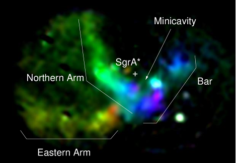
Figure 1: Three-color image of the two mosaicked fields of Sgr A West observed with BEAR in Br$\gamma$, between $-350$ (purple) and $+350$ km s^-1 (red). The standard bright features, Northern and Eastern Arms, Bar, and the Minicavity, are indicated. Also, a few emission line stars show up as bright points in the image.

3 Structure identifications

At each point of the field the Br$\gamma$ and He i emission profiles generally appear complex. The basic assumption is made that each observed profile results from the combination of several velocity components, that is, that along any given line of sight several flows are superposed. The first goal of the present paper is to separate these various flows and to describe them independently from each other. For this purpose, the development of a multi-component line-fitting procedure able to work on 3D data appeared to be absolutely required. From a coarse examination of the datacube, fitting with a maximum of four distinct velocity components along each line of sight seemed adequate.

A comparison of the velocity components from one line of sight to the next should usually reveal coherent velocity structures by continuity. In the end, it might be possible to conclude whether these structures are isolated, or form continuous flows. The process is thus split into two main parts: first the line profile decomposition at all the points of the field, and second, the structure identification. This work is based on original software developed by Miville-Deschênes (personal communication), which we have largely extended.

3.1 Line profile decomposition

3.1.1 Line profile

A single velocity component of the emission lines from the ISM has been assumed to be a Gaussian $I(v)$, with three free parameters: $I_{0}$, the amplitude of the Gaussian expressed in $\mathrm{erg}\cdot\mathrm{s}^{-1}\cdot\mathrm{cm}\cdot\mathrm{pixel}^{-1}$ ($1\ \mathrm{pixel}=0.125\ \mathrm{arcsec}^{2}$); $v_{0}$, the radial velocity of the component; and $\Sigma$, the width of the line, due to thermal agitation, turbulence and any velocity gradient along the line of sight or across a resolution element. The full width at half maximum (FWHM) of the line is given by: $\mathrm{FWHM}=2\Sigma\sqrt{2\ln 2}$.

The instrumental line shape of the FTS is a sinc function:

$$\psi(v)=\frac{\sin\left(\pi\,{\delta_{m}}\,\frac{v\sigma_{0}}{c}\right)}{\pi\,{\delta_{m}}\,\frac{v\sigma_{0}}{c}}$$ (1)

where $\sigma_{0}$ is the central wavenumber and $\delta_{m}$ the maximum path difference between the two arms of the interferometer, which determines the limit of resolution d$\sigma$ of the data with d$\sigma=0.6/\delta_{m}$ (FWHM).

The measured line profile is thus the convolution product $S=I*\psi$, a function of three free parameters $I_{0}$, $\Sigma$ and $v_{0}$. Each single spectrum of the field has been fitted to a set of four such lines, thus implying twelve free parameters.

3.1.2 Procedure

Preparation:

As for any fitting routine, a reasonable initial guess must be provided for each point of the field. For such a problem, where we intend to fit complex line profiles at low signal-to-noise, the method cannot be fully automatic. The operator freely chooses a few starting points, for which he is able to provide an unambiguous decomposition. These starting points should be chosen so that every structure in the field is represented, and keeping in mind that the most complex regions are better fitted if they are close to a starting point. In our case, five starting points were used. From the starting points, a first procedure attempts to fit a four-component line shape function to each spectrum. For each new spectrum, the initial guess is determined from the results found for the neighboring points. The spectra are studied sequentially in parallel spiral-mode scannings around each starting point. Except for the initial guess, the fitting of a spectrum is independent of all the others.

Step 1:

The velocity structures are then built. A totally determinist program finds the brightest point in the field, and examines its neighbors, searching for a component such that the velocity gradient between the point of interest and the neighbor is less than a certain amount, which is set by the operator at runtime. If several velocity components of the examined neighbor spectrum satisfy this velocity gradient criterion, the component with the highest amplitude is assigned to the structure. The procedure is iterative, and once a few neighbors have been selected into a structure, their neighbors are in turn examined for possible selection. A structure is considered to be complete when it cannot be extended any further, that is, when no component of the spectra lying at its border satisfy the gradient criterion. Construction of the next structure is then undertaken, beginning with the brightest point in the data cube not yet selected into a structure. The procedure stops when every component of every spectrum in the field has been assigned to exactly one spatial structure. This procedure allows only one velocity component at any location to be selected into a given structure, and conversely each component at any location can be selected into only one structure. A structure that overlaps itself spatially, thus causing two velocity components along the same line of sight, cannot be directly identified as such: the program splits it into two structures.

Step 2:

The structures containing less than a given number of points, chosen by the operator, are discarded. To be validated, a structure must be more extended than a spatial resolution element, which yields a region more extended than a $3\times 3$ pixel box in our case. After several attempts, we reached the conclusion that no structure containing fewer than $50$ pixels was significant in our field: if such structures exist, their overall signal-to-noise ratio is less than $3\sigma$. The discarded fitted lines corresponding to these abortive structures are either stellar lines, noise spikes, or actual ISM lines under the detection threshold.

Step 3:

This procedure requires that the detected structures be visually inspected. The operator then has the possibility to add some more common sense heuristics into the structure identification, a little difficult to implement but easy to apply manually. Several problems can occur:

• the line fitting procedure might fit only one component where two blended components are indeed more appropriate;

• during step 2, if two overlapping structures intersect in the $\alpha$–$\delta$–velocity space, the procedure can falsely cross-connect them, i.e. reconstruct two structures, each one being made of parts of both physical structures (Fig. 2). The second derivative of the velocity map, as well as continuity of the intensity map, can be used by the operator to decide which connection is the good one. Preliminary work has been done to automatically take these criteria into account.

  

  Figure 2: Cross-connection problem. Left: two physical structures (solid and dashed polygons) intersect each other in the $\alpha$–$\delta$–velocity space. Right: the structures reconstructed by the software can be erroneous.

It is also possible at this time to interpolate the results if they contain holes, and to extrapolate them over a few pixels in order to provide good initial guesses for the next step.

Step 4:

Next, these manually corrected results are used to perform a second fit at each point of the field; at this point, 2D information is entirely included in the initial guess provided to the fitting procedure. Since components have been discarded during step 2, not all initial guesses still contain four components. Steps 1 to 4 can be iterated a number of times to reach a stable result, in our case eight times.

4 Results

4.1 General description of the results

 

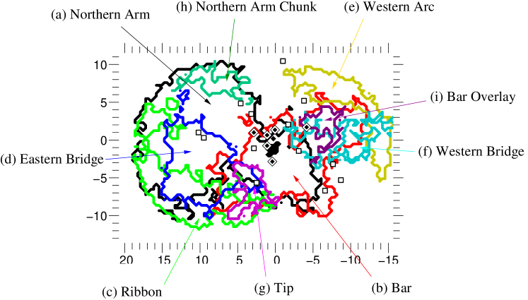
Figure 3: Above: outline of every structure. The region filled in black corresponds to the points where two lines associated with the Northern Arm are detected (see text). Filled diamonds (resp. empty squares) represent narrow (resp. broad) line helium stars. Left: IDs of the narrow (N) and broad (B) line stars, see table below for common-names identification (Paper I, Paumard et al. 2003, and references therein).

ID	Name	ID	Name	ID	Name
N1	GCIRS 16NE	B1	ID~180	B7	AF star
N2	GCIRS 16C	B2	GCIRS 7E2	B8	AF NW
N3	GCIRS 16SW	B3	GCIRS 9W	B9	HeIN3
N4	GCIRS 16NW	B4	GCIRS 15SW	B10	BSD WC9
N5	GCIRS 33SE	B5	GCIRS 13E2	B11	GCIRS 29N
N7	GCIRS 34W	B6	GCIRS 7W	B12	GCIRS 15NE
				B13	GCIRS 16SE2

Both the Br$\gamma$ and He i data have been analyzed with the software described above. This leads to a vision of the Minispiral more complex than usually thought, one which is consistent with, but more detailed than the description proposed by Vollmer & Duschl (2000). After a careful examination of the Br$\gamma$ data we identify 9 components of various sizes, labeled (a) to (i) (Fig. 3). A description of these structures, and their radial velocity and flux maps, are presented in Appendix A. Two types of velocity maps appear, some with a significant overall velocity gradient, others without any appreciable, large-scale velocity gradient. The deviation from the mean motion, defined as the local difference between the velocity measured at one point and the mean value for the neighboring points, and divided by the uncertainty ($3\sigma$ error bars from the multi-component line-fitting procedure), ranges from roughly one tenth to ten for all the features, which means that every velocity structure shows significant local features.

The areal size of the structures (Table 1), expressed in terms of solid angle covered on the sky, ranges from 17 arcsec² to 300 arcsec² for the Northern Arm. The surface area of each structure must be considered as a lower limit because BEAR may not detect the weakest parts, and because the field of view does not cover the entire Minispiral.

Table 1: Feature identifications, with surface areas (pixels and square arcseconds), and minimum and maximum radial velocities (km s^-1). The last column gives [He i]/[Br$\gamma$] for the different structures, relative to the mean value $<$[He i]/[Br$\gamma$]$>$. The Minicavity is separated from the Northern Arm, as it warrants special attention.

ID	Feature name	S (pix)	S (arcsec2)	Vmin	Vmax	[He i]/[Br$\gamma$]
a	Northern Arm	2414	300.8	-290	186	0.74
	Minicavity					0.85
b	Bar	1389	173.1	-214	194	0.99
c	Ribbon	833	103.8	130	240	0.78
d	Eastern Bridge	670	83.5	32	180	1.09
e	Western Arc	471	58.7	-40	72	0.52
f	Western Bridge	327	40.7	-124	98	1.73
g	Tip	207	25.8	220	336	2.64
h	Northern Arm Chunk	185	23.1	12	72	–
i	Bar Overlay	136	16.9	-270	-10	1.81

The same work of decomposition into velocity structures on the He i data was more difficult than for the Br$\gamma$ data since the spectral resolution and signal-to-noise ratio are lower. The fact that the He i data are dominated by the emission from the helium stars also contributes to the greater complexity of this task. We thus skipped the preparatory step of the decomposition process, and provided directly a complete set of initial guesses based on the Br$\gamma$ results, since at first sight the distribution of ionized gas is globally the same in He i. This method precludes the He i analysis from being fully independent, although steps 1 to 4 were performed eight times, until the procedure converged satisfactorily.

Finally, all the structures detected in Br$\gamma$ are detected in He i as well, except the Northern Arm Chunk (h), which is probably too weak in this line. However, several differences in the appearance of these structures are noticeable, and detailed in Appendix B. To quantify these differences, we have built [He i]/[Br$\gamma$] line ratio maps for each structure, normalized to the areal mean for this ratio over the union of all the structures. The [He i]/[Br$\gamma$] line ratio varies considerably across the field, so that, for instance, the Northern Arm bright rim and the Minicavity do not show the same shape in He i and Br$\gamma$ (Fig. 4). The last column of Table 1 shows the mean normalized [He i]/[Br$\gamma$] line ratio for the different structures. It appears that this ratio is lower than the mean value for the main, well-known features – the Northern Arm, the Ribbon, the Bar and the Western Arc – and higher for the smaller features. However, the values are computed only for the positions detected in both Br$\gamma$ and He i, so they do not take into account the faintest, least excited regions of each feature.

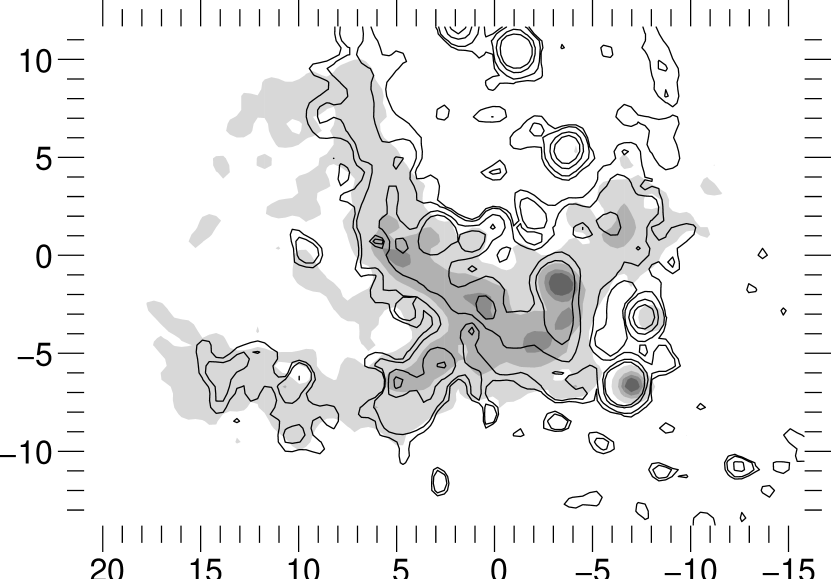
Figure 4: Comparison between integrated flux in Br$\gamma$ (grey scale) and He i (empty contours). Axes are offsets from Sgr A^⋆ in arcsec.

4.2 Brief description of the main features

Although all nine structures are thoroughly described in Appendices A and B, we briefly summarize here the most important results. Contrary to its standard description, the Northern Arm is not seen here as a bright N-S lane, but as an extended, triangular surface. One edge of this triangle is the bright rim generally noticed, but it extends all the way over to the Eastern Arm. The third edge of the triangle is the edge of the field, so viewing this feature in a larger field may yield a somewhat different description. It contains the Minicavity. The [He i]/[Br$\gamma$] line ratio is higher on the western side of the bright rim of the Northern Arm and on the inner side of the Minicavity than in the rest of the structure.

As already described by Vollmer & Duschl (2000), the Eastern Arm region is split into two parts: a Ribbon (c) and a Tip (g). For the sake of clarity, we chose not to name any feature “Eastern Arm”. At the elbow between the Ribbon and the Tip, in the GCIRS~9W region, is a bubble-like feature, or a Microcavity (radius $\simeq 1\arcsec$), with a rather bright rim (Fig. 5), which appears at a specific velocity (230 km s^-1). Finally, a secondary rim parallel to the Eastern Arm (Fig. 8, from spot A eastwards) is often associated with it. Here, we see that this feature belongs to an independent structure, the Eastern Bridge (d).

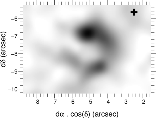
Figure 5: Microcavity feature in the region of GCIRS 9W, represented by the black cross. Axes are offsets from Sgr A^⋆. Integrated velocity range: $220$–$240$ km s^-1.

4.3 Extinction by the structures

One of the most difficult questions concerning the ionized features is to determine their relative positions, i.e., when two structures overlap, which one is closer to the observer. On two occasions, the flux maps can be used to infer this information.

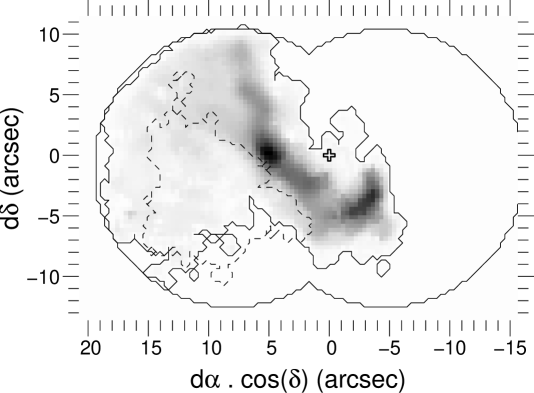
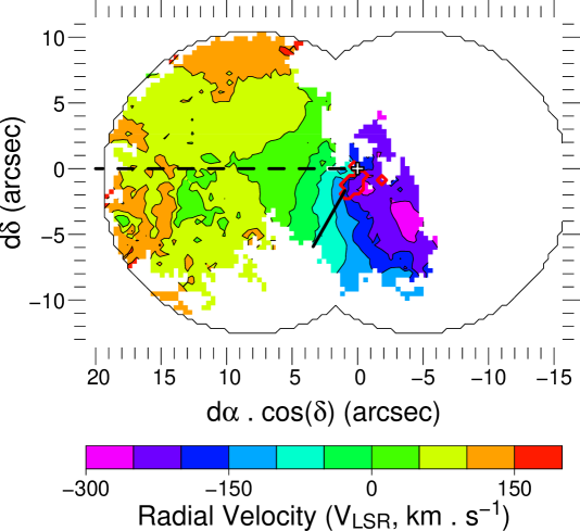
Figure 9: (a) Northern Arm.

The flux map of the Northern Arm (Fig. 9) shows a region of low intensity, the northwestern boundary of which is a well defined line, oriented approximately northeast–southwest. This intensity discontinuity is most obvious south of GCIRS~1 and west of the Minicavity. This line follows very closely the outline of the Eastern Bridge. It goes from $\simeq 2\arcsec$ east and $5\arcsec$ south to $13\arcsec$ east and $3\arcsec$ north of Sgr A^⋆, where it becomes more difficult to locate precisely because of a lower signal-to-noise ratio. If we interpret the intensity discontinuity in terms of an increment of the extinction, this gives us two pieces of information: the Northern Arm is behind the Eastern Bridge on the line-of-sight, and the Eastern Bridge contains a substantial amount of dust, responsible for the extinction of about $50\%$ of the Br$\gamma$ flux of the Northern Arm, or about $\simeq 0.76$ magnitudes at K. The ratio of K extinction to visual extinction being about $0.1$, the inferred visual extinction is around $7.6$ magnitudes. Using the area of the Eastern Bridge, 83.5 arcsec² (Table 1), and the conversion factor of $2\times 10^{21}$ cm^-2 per visual magnitude of extinction, we estimate the mass of the Eastern Bridge to be $\simeq 15$ M_⊙. This estimate is to be considered with caution since the conversion factor may be different in this extreme environment, and since we have only one measurement point for the extinction, although the Br$\gamma$ emission seems to correlate well with the extinction map inferred from the Northen Arm’s emission map, which is difficult to interpret. Furthermore, this estimate does not include a possible extension of the Eastern Bridge outside our field of view. However, it is comparable to the mass of $\simeq 27$ M_⊙ estimated by Liszt (2003) for the Bar.

Although the flux map of the Bar (Fig. 10) is less smooth than that of the Northern Arm, making such effects more difficult to see, the shape of the periphery of the Minicavity is clearly identified in extinction on this map, showing that the Bar is behind the Northern Arm along the line of sight.

5 Keplerian orbit fitting

The velocity maps give a view of the features very different from the usual flux maps which, by themselves, can be misleading. For instance the morphology of the Northern Arm with its typical rim may lead one to think of this rim as the true path for most of the material, whereas the velocity map does not show any peculiar feature at the location of the rim. We are thus led to the idea that the kinematics of the Northern Arm should be studied independently of its intensity distribution. To do so, we have tried to analyze the Northern Arm as a Keplerian system, the location and mass of the central object being those of Sgr A^⋆. Its position with respect to GCIRS~7 is taken from Menten et al. (1997), and the positions of the stars in the field relative to GCIRS~7 from Ott et al. (1999). The distance to SgrA* is the value of 8 kpc reported by Reid (1993). We have used a mass of $3\,10^{6}$ M_⊙ for most of our models, and we will discuss the impact of changing this mass later.

5.1 Fitting one orbit on a velocity map

For a first, simple approach, we created a dedicated IDL graphical package. With this tool, the operator can easily adjust one Keplerian orbit over a velocity map. A Keplerian orbit in 3D is defined by five orbital parameters: the eccentricity, two angles defining the orientation of the orbital plane, the periapse (distance of closest approach to the center of motion), and a third angle defining the position of the periapse.

Once the operator is almost satisfied with the orbital parameters found by trial and error, an automatic fitting procedure can be called. It is possible to fix parameters, and the orbit can be forced to go through a selected constraint point by tying the periapse to the other parameters. Good agreement can be found between observed and calculated velocities, except in the region of the Minicavity, so we attempted to model the full velocity field of the Northern Arm with a bundle of Keplerian orbits bounded by various constraints. We note that this model alone is not sufficient to decide whether the orbits are bound to the gravitational field of the black hole, since the bound and unbound solutions are not dramatically different within our field of view.

5.2 Fitting a bundle of orbits on a velocity map

To fit several orbits at a time on a velocity map, we force each one to pass through a different constraint point, as in the one-orbit case, with the constraint points chosen to be on different physical orbits. The result described here uses 50 constraint points, evenly spaced on the solid line of Fig. 9. Another constraint line has been tried as well (dashed line), with consistent results. Each constraint point is given an index, increasing from the point nearest Sgr A^⋆ outwards, that is used to refer to a given orbit.

To ensure a smooth model – we are interested only in the global motion – the four functions that map each constraint point to one of the orbital parameters have been chosen to be described as spline functions, uniquely defined by their value at a number of control points, chosen among the constraint points. The number of points used to define the spline function can be freely chosen to set the spatial resolution of the model across the flow. After several attempts, we have chosen to fix this number to four in our final model (yielding a resolution of $8.8\arcsec$). Thus, having four functions (one for each of the orbital parameters), each of them being defined by four values, the model depends on sixteen parameters.

We designed a fitting procedure to adjust this model based on the observed velocity map by minimizing the reduced $<\!\chi^{2}\!\!>$. It is possible to either fix some parameters, or to force them to have the same value for each orbit. This way, for example, it is possible to check whether the observed velocity map is consistent with coplanar orbits or with uniform eccentricity. To avoid studying only local minima in the parameter space, it is also important to use several initial guesses.

5.3 Homothetic hypothesis

We again designed an IDL graphical tool to easily study whether the data are consistent with a homothetic set of orbits, which is the simplest model.

With the hypothesis of a homothetic set of orbits, the eccentricity still cannot be well constrained. Bound orbits seem to be preferred, but the agreement is as good with circular orbits and very eccentric orbits, close to parabolic. The residual map always has the same shape: the observed velocities are always smaller than the computed ones along the inner edge of the bundle of orbits, and higher along the outer edge. The global agreement is always poor, with $<\!\chi^{2}\!\!>^{1/2}\simeq 70$.

5.4 General case

A few of these homothetic models have been chosen as initial guesses for other adjustments, with released constraints. It is first interesting to check the coplanar hypothesis, in which only the two parameters that define the orbital plane are kept uniform, and the uniform eccentricity hypothesis. The agreement is much better when leaving either the eccentricity or the orbital plane free. In the following, both parameters are free.

Even in the most general situation, the parameters are still not constrained enough to extrapolate the model outside the field of view, or to derive reliably the direction of proper motion. However, the models share a few characteristics that we judge to be robust because of their repeatability: the orbital planes are close to that of the CND; the orbits are not quite coplanar, the two angles that define the orbital plane varying over a $\simeq 10^{\circ}$ range; the eccentricity varies from one orbit to another, the innermost orbits being hyperbolic ($e$ of the order of 2) and the outermost closer to circular ($e\lesssim 0.5$).

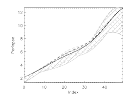
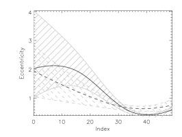
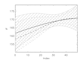
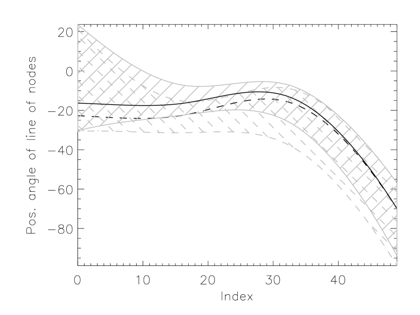
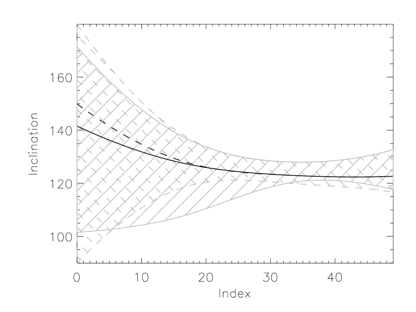
Figure 6: These five plots show the laws of each of the five orbital parameters in our two best models. Solid lines: $M_{\mathrm{SgrA*}}=3\,10^{6}\,\mathrm{M}_{\odot}$. Dashed lines: $M_{\mathrm{SgrA*}}=4\,10^{6}\,\mathrm{M}_{\odot}$. The gray hashed regions correspond to the $2\sigma$ error bars. Angles are in degrees, the periapse in equivalent arcsec on the sky.

5.5 3D morphology and time-scale of the Northern Arm

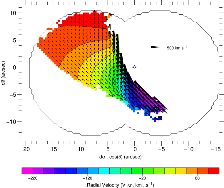
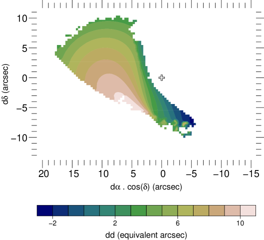
Figure 7: Above: 3D velocity map for the Northern Arm from our model. The arrows show the derived tangential velocities. Left: elevation map for the detected part of the Northern Arm from our model, given in equivalent arcseconds for homogeneity. d$d$ stands for differential of the distance, positive d$d$ means further away from the observer than the center of mass, Sgr A^⋆, at d$\alpha=0$, d$\delta=0$, d$d=0$.

We present here our best model, i.e., the one with the lowest $<\!\chi^{2}\!\!>^{1/2}$ among the realistic models that cover most of the Northern Arm. The laws used for this model are shown in Fig. 6. The agreement between the radial velocity map of this model and the observed velocity map is good: $<\!\chi^{2}\!\!>^{1/2}=18$. The histogram of the radial velocity difference between our model and measurements is close to a Gaussian distribution centered on zero with $\sigma=10$ km s^-1. That means that the method is unbiased, and that the mean error is 10 km s^-1. Figure 7, also available at CDS in FITS format, shows the 3D velocity map of the Northern Arm derived from this model. The FITS version consists of four FITS files. The first gives the geometry of the cloud by means of the distance to the observer at each point of the field; the second contains a stack of three maps, each one giving one velocity component. The two other files give the error bars for the two first files.

The variations of the orbital parameters induce a particular 3D shape for the Northern Arm (Fig. 8): for all the non-coplanar models, the Northern Arm looks like a saddle-shaped surface, and this warped shape induces a crowding of orbits that closely follows the bright rim of the structure. Two different geometries could explain this saddle shape: the Northern Arm could be a warped planar structure, or have approximately the shape of the inner side of a torus. An infalling neutral cloud, tidally stretched by the black hole, would have such a torus-like geometry. If, in addition, its inner side was ionized by hot stars located still further inside, near the black hole, as the GCIRS~16 stars are, one must expect this ionized skin to have precisely the same saddle shape as the Northern Arm. The bright rim itself is not only due to the stronger UV field and a real local enhancement of the density, but also to an enhancement of the column density due to the warping. An interesting point is that, in some models, no orbit follows the bright rim, which emphasizes that it is really important to consider the dynamics independently from the morphology of the Northern Arm. Another characteristic present in all models is that the period of the orbits ranges from a few $10^{4}$ years to a few $10^{5}$ years, which implies that the Northern Arm would have a completely different shape in a few $10^{4}$ years, and cannot be much older than that time-scale. These results are in good agreement with the conclusions of the model of Sanders (1998) for explaining the observed structure of the ionized gas filaments, in particular the Northern Arm, explained in term of disruption of gas clouds in the potential of a point mass.

Since the agreement in radial velocity is now rather good, it makes sense to look at the deviations from global motion by looking at the features on the residual velocity map (Fig. 8):

A)

the flow shows a rather significant deviation in the region just southwest of the embedded star, GCIRS~1W; this perturbation could be due to the interaction with the wind of this star; indeed a bow shock where the wind meets the ambient Northern Arm gas has been invoked to explain the observed morphology of GCIRS~1 (Tanner et al. 2004).

B)

the region of this model closest to the Minicavity is perturbed;

C)

another deviation is seen at the precise location where the bright rim bends abruptly, just east of GCIRS~7E2;

D)

finally, an elongated feature is seen on the fainter rim coming from GCIRS~1W towards the northeast.

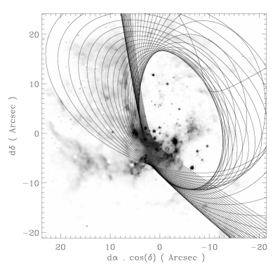
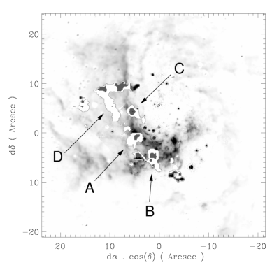
a) b)

Figure 8: a) on this Pa$\alpha$ map (Scoville et al. 2003), one of the Keplerian models is overplotted. b) the most significant deviations from Keplerian motion discussed in the text are labeled A to D, and indicated as filled contour.

6 Discussion

The geometry of the Northern Arm has been studied from its velocity map, leading to the conclusion that it may not be planar, but rather is a three-dimensional structure. The best model discussed above, which uses a central mass of $3\times 10^{6}$ M_⊙, has been used as the initial guess for another adjustment using $4\times 10^{6}$ M_⊙. With this value of the central mass, every remark made above is still valid. The $<\!\chi^{2}\!\!>$ is slightly degraded, but not significantly changed. This analysis cannot provide stringent constraints on the central mass.

Figure 8a is quite compatible with the Northern Arm indeed being the ionized surface of a neutral cloud (as suggested by Jackson et al. 1993; Telesco et al. 1996). This figure also suggests that the Northern Arm and the Western Arc may be two parts of the same physical structure. The velocity derived from the model agrees with the measured velocity of the Western Arc within $\simeq 50$ km s^-1 (which is reasonable since it is an extrapolation) and has the right gradient, but this coincidence is lost when a central mass of $4\times 10^{6}$ M_⊙ is used. However, the adjustment is not made over the entire Northern Arm, since our field of view is limited. The same study on a complete map of the Northern Arm would probably show whether the Northern Arm and Western Arc are one and the same physical feature. In any case, the orbital plane of the Northern Arm is very close to that of the CND, which suggests that the Northern Arm may have originated from a cloud in a stable orbit inside the CND, which would have been extracted from there through a cloud-cloud collision for instance. However, from their study of proper motions of features in the Minispiral, Yusef-Zadeh et al. (1998) show that some material of the Northern Arm seems to be on hyperbolic orbits, which we confirm, and which implies that the captured clouds lose some mass in their process of evolution into long filaments. The tangential velocity field of the Northern Arm (Fig. 7) is interestingly similar to the magnetic field derived by Aitken et al. (1998), which is easily explained by the shear in our model.

We have shown that at least two structures are thick, dusty clouds, because their extinction factor is of the order of several $10\%$ at $2$ $\mu$m: the Eastern Bridge and the edges of the Minicavity in the Northern Arm. From the wider field in Pa$\alpha$, we can assume that the Eastern Bridge is an east-west elongated cloud, of which only the western part is in the field of view of BEAR. If this cloud is moving westwards along its principal axis, this western part must be the leading side of the cloud along its orbit, which would explain the lack of shear inferred from its velocity map.

The presence of three isolated ionized gas structures (the Western Bridge, the Northern Arm Chunk and the Bar Overlay) in addition to the standard large flows and to the Eastern Bridge, which seems to be another flow, has been demonstrated. Some of these structures may be isolated gas patches, but it is also possible that some of them are regions of the neutral clouds in which ionized fronts form the Minispiral, locally excited. For instance, the Bar Overlay, the velocity map for which is very similar to that of the Bar, may be a region belonging to the same neutral cloud as the Bar, which would be locally excited by GCIRS~34W. The [He i]/[Br$\gamma$] line ratio is significantly higher for these tenuous features than for the standard Northern Arm, Eastern Arm and Bar. This ratio is variable across each structure, which can basically be explained in two ways: first, it can be the trace of local enrichment of the gas in helium, and second, it can be due to local enhancements of the excitation, either because of a stronger UV field or of shocks.

There are about $20$ high mass loss stars in the region (Paper I and references therein). A typical mass loss rate for stars of these spectral types is of the order of $\simeq 10^{-4}$ M_⊙ yr^-1 (Najarro et al. 1994). This material must reside in the central parsec for a duration similar to the time-scale of the Northern Arm: $\simeq 10^{4}$ yr. From these considerations, the total mass of interstellar gas in the central parsec coming from the mass loss of these stars must be around a few tens of solar masses. On the other hand, if the ionized structures are really the ionized fronts of neutral clouds, these clouds could have a mass similar to that of the clouds that form the CND: $\simeq 10^{3}$ M_⊙ each (Christopher & Scoville 2003). It would then be unlikely that interstellar gas of stellar origin contribute significantly to the enrichment of these clouds. However, such a significant contribution remains plausible if the individual structures are indeed much less massive than $10^{3}$ M_⊙, as suggested in Sect. 4.3.

There is a clear correlation between the projected proximity of gas to the helium stars and the [He i]/[Br$\gamma$] line ratio:

• two of the gas patches detected in both lines having a high [He i]/[Br$\gamma$] ratio are coincident with the helium star GCIRS~34W;

• the Bar, which is the main feature with the highest line ratio, is close to the GCIRS~16 helium star cluster, and seems to contain the GCIRS~13E star cluster (Appendix A), which is made of several high-mass-loss-rate stars (Maillard et al. 2004);

• the Tip, the feature with the highest [He i]/[Br$\gamma$] ratio, seems to be interacting with a stellar wind, as evidenced by the Microcavity, and is on the same line of sight as the helium star GCIRS~9W;

• the differences in the shape of the Northern Arm between the two spectral lines appear to come from the geometry of the UV field around the GCIRS~16 cluster.

The discrepancies that are most difficult to explain are the high brightness in He i, in contrast to their relative faintness in Br$\gamma$ in the southwestern parts of both the Minicavity and the Tip. However, this part of the Minicavity is rather close in projection to the AF star, the flux of which, if this proximity is not only in projection, could favor He i emission. Finally, our results remain consistent with interstellar material of uniform composition, distributed in a non-uniform UV field, the exact value at any given point depending on the 3D localization of nearby hot stars.

In addition to this, a Microcavity has been discovered at the elbow between the Eastern Arm Ribbon and Tip. It is probably a new example of interaction between stellar wind or polar jet and an ISM cloud, similar to the Minicavity. Another apparent star-ISM interaction phenomenon is the interaction of the Northern Arm gas flow with GCIRS~1W (spot A in Fig. 8b). These interactions show that the dynamics of the flows must be influenced by the stars, as Yusef-Zadeh & Wardle (1993) suggested for the wind of the GCIRS~16 cluster.

7 Conclusion

We begin to gain access to the relative positions of features along the line of sight: the Eastern Bridge is closer to the observer than the Northern Arm, and the Bar is behind the Northern Arm. In addition to that, knowledge of the radial velocity field of the Northern Arm has allowed us to propose a kinematic model, which provides a three dimensional map of this feature. Having such maps for all of the ISM features would give us the opportunity to estimate the UV field that hits these ISM features, taking the shadowing effects into account. It would then become possible to estimate the helium abundance in the different structures from their relative line ratios. and to assess the notion that these structures have incorporated enriched material processed through the post-main sequence stages of evolution of massive stars and then ejected as winds.

This work has been performed on a field covering most of the inner parts of the Minispiral. However, repeating the same analysis on a wider field containing the Minispiral to its full extent, would allow one to directly check whether the Northern Arm and the Western Arc are related features, an important constraint on their formation scenario. Moreover, obtaining the velocity maps of a wider field would allow one to better constrain the parameters of the Keplerian fit to the Northern Arm, and may then reveal deviations from the Keplerian model, due to momentum loss or to non-gravitational forces. This would be a very interesting clue to the accretion process. This program requires a wide-field spectro-imager with spectral and spatial resolutions comparable to those of BEAR.

Appendix A Morphology of the ionized gas in Sgr A West

A description based on the analysis of the Br$\gamma$ data follows for each identified velocity structure. Their Br$\gamma$ line flux (peak intensity $\times$ width of the line) and radial velocity maps are given in Figs. 9 to 16. Axes show offsets from Sgr A^⋆ (represented as a cross), in arcseconds. The line flux maps are the gray scale images, left-hand column; a black outline gives the full extent of the detected structure. The velocity maps are the color level images, right-hand column; to improve contrast, the color scale is not the same for each map. The binocular-shaped black line shows approximately the field boundaries.

(a) Northern Arm (Fig. 9): It extends from its well known bright N-S lane all the way over to the Eastern Arm. The third edge of this triangularly shaped feature is the edge of the field. Its flux is partly absorbed (Sect. 4.3) by the Eastern Bridge, the outline of which is shown as a dashed line on the Northern Arm flux map. As it reaches the Minicavity, the Northern Arm is split into two layers in the spectral direction: on the spectra of a few adjacent pixels (14), two lines are clearly detected, indicating two layers of gas that both connect continuously with the rest of the Northern Arm (each layer is separately found by our software described Sect. 3.1.2). The main layer contains all of the Minicavity, while the second layer seems to be deflected northward of the Minicavity, and forms the small finger between the two helium stars GCIRS~16SW (N3) and GCIRS~33SE (N5, Fig. 3). It extends further away by $\sim 5\arcsec$ to the northwest, and contains the point-like feature just above the aperture of the Minicavity (source $\epsilon$ of Yusef-Zadeh et al. 1990). On the few pixels where both features are detected, the secondary layer is $50$–$80$ km s^-1 more blueshifted than the main one. Both layers are represented in the velocity maps (Figs. 7 and 9), indicating the velocity of the secondary one for the few points outlined in red, where both are detected. The flux map (Fig. 9) gives the sum of the two layers. The direction of the Northern Arm motion (from north to south) has been established by Yusef-Zadeh et al. (1998). The kinematics of the Northern Arm are thoroughly discussed in Sect. 5. In the velocity map, the two straight lines represent the constraint lines used for our Keplerian models (Sect. 5.2).

(b) Bar (Fig. 10): It is very extended (from the Ribbon of the Eastern Arm (c) to the Western Arc (e)), very straight, and shows a smooth overall velocity gradient. Its flux is partly absorbed by the edges of the Minicavity (Sect. 4.3), a few contours of which are given as dotted lines in the flux map of the Bar. The map peaks sharply at the location of the GCIRS~13E compact star cluster (Maillard et al. 2004), which seems to show that this object excites local material in the Bar, and thus must be either embedded in it, or very close to it. Thus, the coincidence between this bright spot and the northern end of the western edge of the Minicavity seems to be a projection effect, and not physical. Vollmer & Duschl (2000) mention two complementary components of the Bar, which they call Bar~1 and Bar~2, though their description is not sufficient to determine precisely the positions of these two suggested components. We also see two additional features, which we propose to call the Western Bridge (f) and Bar Overlay (i). Parts of the Bar are also superimposed on almost every other structure, including the Ribbon of the Eastern Arm (c), the Tip (g), the Eastern Bridge (d) and the Northern Arm (a).

(c) Ribbon (Fig. 11): As already described by Vollmer & Duschl (2000), the Eastern Arm region is split into two parts: a Ribbon and a Tip (g). The velocity gradient of the Ribbon is directed along the minor axis of the structure, not along its major axis as expected for a flow.

(d) Eastern Bridge (Fig. 12): A structure of medium size extends from the Ribbon (c) to the bright rim of the Northern Arm. It does not show any large-scale velocity gradient, and its shape does not show any principal axis that would indicate a flow. It is superimposed on the faint regions of the Northern Arm, and partly superimposed on the Ribbon, the Bar and the Tip. Its southern side is parallel to, as well as superimposed upon, the Ribbon; the two structures are probably related, although their relative velocities differ by more than 50 km s^-1. The name we propose is based on the fact that it lies between the two Arms of the Minispiral, both in the spatial and spectral dimensions, being close to the Ribbon in the spectral dimension on its southern side and to the Northern Arm on its northern side. It is also inspired by the fact that the most luminous part of it in our field is a small vertical bar, seemingly connecting the bright parts of the Northern and Eastern Arms. This bar is located around $7\arcsec$ east of Sgr A^⋆, and extends from about $1$ to $6\arcsec$ south of Sgr A^⋆. However, the Pa$\alpha$ map (Fig. 8) shows that this bar may extend outside our field-of-view into an elongated feature parallel to the Ribbon, going from about $7\arcsec$ east and $1\arcsec$ south to $\simeq 23\arcsec$ east and $9\arcsec$ north of Sgr A^⋆. The lack of an overall gradient in the velocity map suggests that this feature is not much affected by shear. It seems related to the entity formed by the combination of the Ribbon and the Tip; it may belong to it, or be interacting with it.

(e) Western Arc (Fig. 13): The Western Arc lies just at the edge of the field, so we have access only to its innermost part. It is seen as a rather simple feature, with large scale velocity gradient. It is superimposed on the Western Bridge on a few pixels. The velocity field that we measure is basically in good agreement with that of Lacy et al. (1991).

(f) Western Bridge (Fig. 14): The Western Bridge is a tenuous, elongated feature oriented east-west and extending from the Bar to the Western Arc. This structure, as well as the Bar and the Bar Overlay (i) upon which it is superimposed, contains in projection the helium star GCIRS~34W (N7, Fig. 3).

(g) Tip (Fig. 15): The Tip is, in projection, a very concentrated and relatively small object with the most redward velocity in the region ($\simeq 300$ km s^-1). The Tip has already been noticed by Vollmer & Duschl (2000) only on a morphological basis, as a finger-shaped portion of the Eastern Arm in their three-dimensional data. Here, we see that the Ribbon and the Tip are two distinct features, superimposed on the line of sight (we detect two lines on $72$ lines-of-sight), and separated by a Microcavity (Fig. 5), thus we do not adopt the representation-dependent denomination “Finger”.

(h) Northern Arm Chunk (Fig. 16): A small tenuous structure is seen superimposed on the Northern Arm, a few arcseconds north of GCIRS~7. It lies at the edge of our field, so it could extend further out; however the Pa$\alpha$ image shows a small, horizontal bar at its location, crossing the bright rim of the Northern Arm, that does not seem to be much extended.

(i) Bar Overlay (Fig. 16): The Bar Overlay looks like a small cloud that is superimposed upon the western region of the Bar and that shows a velocity gradient similar to the one of the main Bar at the same location, with an offset of $\simeq-40$ km s^-1. This may indicate that these two features are closely related. They could, for example, be the two faces of a single neutral cloud, ionized by two distinct UV sources.

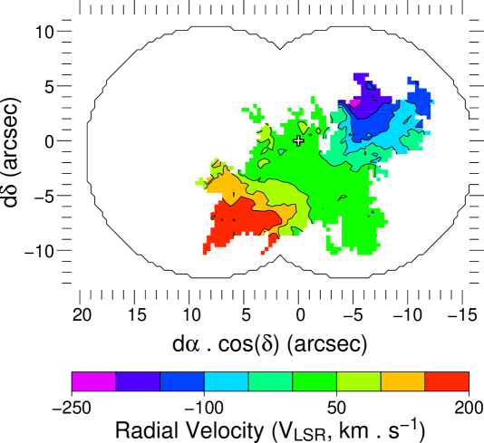
Figure 10: (b) Bar.

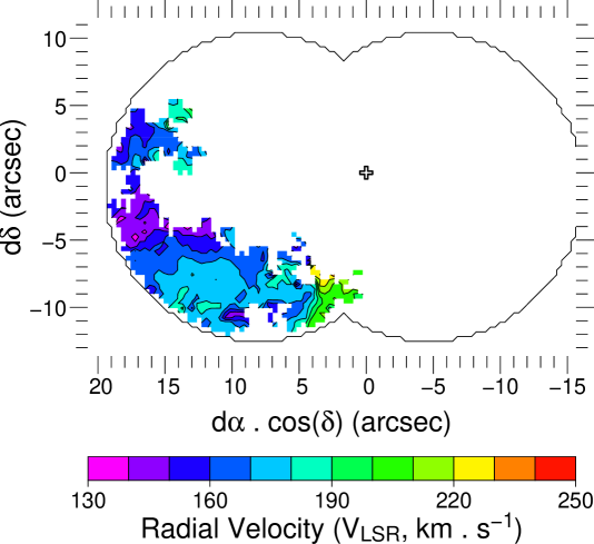
Figure 11: (c) Ribbon.

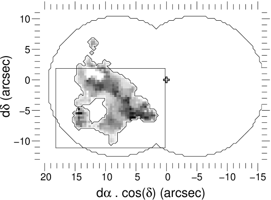
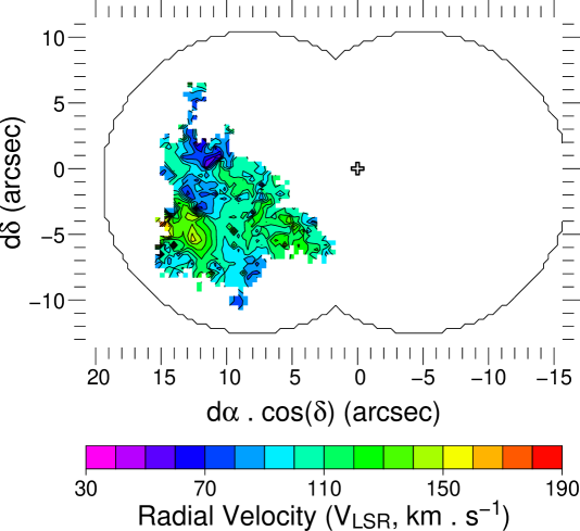
Figure 12: (d) Eastern Bridge. The box shows the field of Fig. 17.

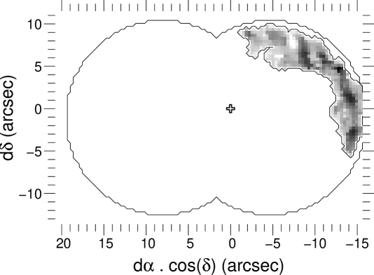
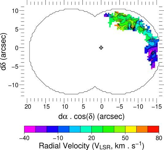
Figure 13: (e) Western Arc.

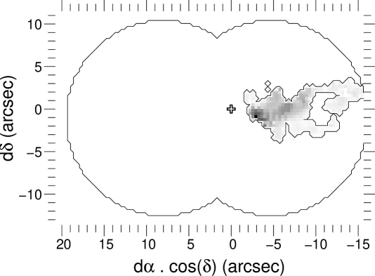
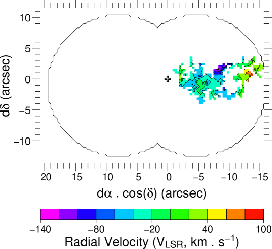
Figure 14: (f) Western Bridge.

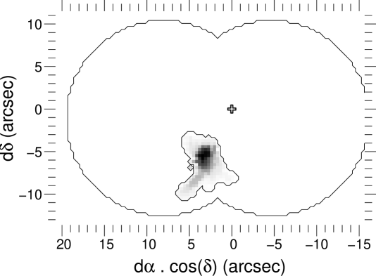
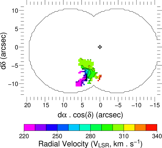
Figure 15: (g) Tip.

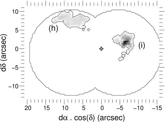
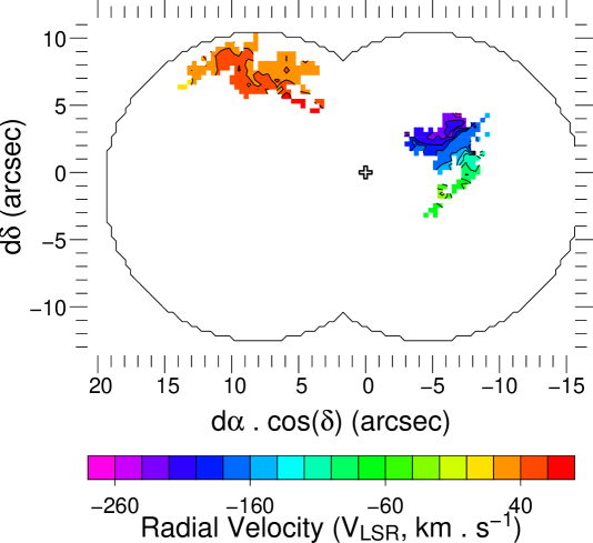
Figure 16: (h) Northern Arm Chunk and (i) Bar Overlay.

Appendix B Comparison with He i data

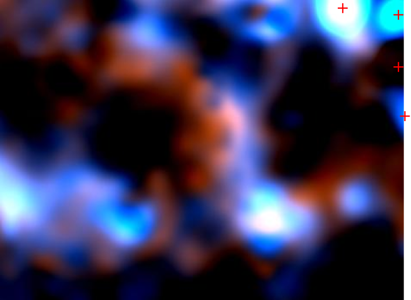
Figure 17: Composite image of the Eastern Bridge, from images integrated from 50 to 100 km s^-1 in the Br$\gamma$ (red) and He i (blue) cubes. The positions of four helium stars at the upper right corner are given by red crosses (GCIRS~16NE, 16C, 16SW and 33SE). The field is shown in Fig. 12.

(a) Though the Northern Arm remains the most prominent feature of the Minispiral, the mean value of its normalized [He i]/[Br$\gamma$] line ratio (Minicavity excluded) is one of the lowest ($\simeq 0.74$), being only higher than the value measured for the small part of the Western Arc that we detect. Considering that the faintest parts of the Northern Arm are not detected in He i, this value may be even smaller. The line ratio is higher on the western side of the bright rim, and in He i this rim has the shape of a part of a circle surrounding the GCIRS~16 cluster. This circle continues further to the northwest, forming a rather faint horn at the location where, in Br$\gamma$, the rim bends abruptly ($5\arcsec$ to the north and $5\arcsec$ to the east of Sgr A^⋆, spot C on Fig. 8).
The open ring of ionized gas surrounding the Minicavity is on average brighter in He i than the rest of the Northern Arm relative to the intensity distribution in Br$\gamma$. Its innermost border is even brighter. Its western edge, where GCIRS~13 and GCIRS~2 lie, is very bright, and looks like a vertical bar going from GCIRS~13 almost to the declination of the AF star, making the Minicavity look angular. Physical implications of these variations of the line ratio are discussed in Sect. 6.

(b) The Bar is the main feature with the highest [He i]/[Br$\gamma$] ratio, with a normalized value of 0.99. However, we do not detect helium towards the full extent of its Br$\gamma$ counterpart.

(d) The Eastern Bridge (Fig. 17) is clearly identified, but it presents a shape much different from the one observed in Br$\gamma$. It is brighter on its southern side, and the northern parts are not detected by the procedure. The southern parts extend horizontally, following the edge of the Eastern Arm Ribbon upon which it is superimposed, with a velocity offset between the Eastern Bridge and the Ribbon of about -50 km s^-1 (measured in Br$\gamma$, but the agreement is good between the two lines), which again suggests that the two features are related. The bow-shaped bright rim of the structure, which is almost vertical and gives its name to the Eastern Bridge, is offset in He i by about $1\arcsec$ to the West relative to Br$\gamma$.

(e) A small part of the Western Arc is detected within our field; its [He i]/[Br$\gamma$] value is the smallest, but only a few points are detected both in He i and Br$\gamma$.

(g) Due to the lower spectral resolution of the He i data (52.9 km s^-1, vs. 21.3 km s^-1 in Br$\gamma$), the Tip is not separated from the Ribbon by our procedure in this band. However, it is clearly seen. It is the brightest feature relative to its Br$\gamma$ counterpart, with a normalized line ratio of $\simeq 2.64$. The line ratio is also noticeably brighter on its southwestern edge than on its northeastern edge, which is not detected in He i by the decomposition procedure. The Microcavity is also observed in He i.