The ACS Virgo Cluster Survey III. Chandra and HST Observations of Low-Mass X-Ray Binaries and Globular Clusters in M87

Abstract

The ACIS instrument on board the Chandra X-ray Observatory has been used to carry out the first systematic study of low-mass X-ray binaries (LMXBs) in M87, the giant elliptical galaxy near the dynamical center of the Virgo Cluster. These images — having a total exposure time of 154 ks — are the deepest X-ray observations yet obtained of M87. We identify 174 X-ray point-sources, of which $\sim$ 150 are likely LMXBs. This LMXB catalog is combined with deep F475W and F850LP images taken with ACS on HST (as part of the ACS Virgo Cluster Survey) to examine the connection between LMXBs and globular clusters in M87. Of the 1688 globular clusters in our catalog, $f_{X}=3.6\pm$0.5% contain a LMXB. Dividing the globular cluster sample by metallicity, we find that the metal-rich clusters are 3$\pm$1 times more likely to harbor a LMXB than their metal-poor counterparts. In agreement with previous findings for other galaxies based on smaller LMXB samples, we find the efficiency of LMXB formation to scale with both cluster metallicity, $Z$, and luminosity, in the sense that brighter, more metal-rich clusters are more likely to contain a LMXB. For the first time, however, we are able to demonstrate that the probability, $p_{X}$, that a given cluster will contain a LMXB depends sensitively on the dynamical properties of the host cluster. Specifically, we use the HST images to measure the half-light radius, concentration index and central density, $\rho_{0}$, for each globular, and define a parameter, $\Gamma$, which is related to the tidal capture and binary-neutron star exchange rate. Our preferred form for $p_{X}$ is then $p_{X}\propto\Gamma\rho_{0}^{-0.42\pm 0.11}(Z/Z_{\odot})^{0.33\pm 0.1}.$ We argue that if the form of $p_{X}$ is determined by dynamical processes, then the observed metallicity dependence is a consequence of an increased number of neutron stars per unit mass in metal-rich globular clusters. Finally, we present a critical examination of the LMXB luminosity function in M87 and re-examine the published LMXB luminosity functions for M49 and NGC 4697. We find no compelling evidence for a break in the luminosity distribution of resolved X-ray point sources in any of these galaxies. Instead, the LMXB luminosity function in all three galaxies is well described by a power law with an upper cutoff at $L_{X}\sim 10^{39}$ erg s^-1.

1. Introduction

Normal elliptical galaxies have long been known to harbor two major components of X-ray emission — a soft component due to emission from diffuse gas, and a harder one arising from a population of low-mass X-ray binaries (LMXBs). The existence of the latter component was first inferred from the spectral hardening of elliptical galaxies with progressively smaller X-ray to optical luminosities, a trend reminiscent of late-type galaxies in which a portion of the X-ray emission could be identified directly with a population of accreting binary stars (Kim, Fabbiano & Trinchieri 1992). With the launch of Chandra, the harder X-Ray component has been partially resolved into point sources associated with LMXBs for an ever-increasing number of early-type galaxies ($e.g.$, Sarazin, Irwin & Bregman 2001, 2002; Angelini, Loewenstein & Mushotzky 2001; Blanton, Sarazin & Irwin 2001; Finoguenov & Jones 2002; Kundu, Maccarone & Zepf 2002; Maccarone, Kundu & Zepf 2003; Kundu et al. 2003; Jeltema et al. 2003; Kim & Fabbiano 2003; Irwin, Athey & Bregman 2003; Sivakoff, Sarazin & Irwin 2003).

In the Milky Way, it was realized soon after the discovery of X-ray emission from a handful of Galactic globular clusters (GCs) (Giacconi et al. 1974; Forman et al. 1978) that the number of X-ray sources per unit mass is several hundred times higher in GCs than in the halo field (Katz 1975; Clark 1975). The population of X-ray point sources associated with GCs was later found to be a mixture of dim ($L_{X}\mathrel{<\kern-10.00002pt\lower 3.87495pt\hbox{$\sim$}}10^{34.5}$ erg s^-1) and bright ($10^{36}\mathrel{<\kern-10.00002pt\lower 3.87495pt\hbox{$\sim$}}L_{X}\mathrel{<\kern-10.00002pt\lower 3.87495pt\hbox{$\sim$}}10^{38}$ erg s^-1) sources (Hertz & Grindlay 1983). The fainter sources seem to be composed of many different kinds of objects (see, $e.g.$, Verbunt 2001), while the bright sources are believed to be accreting neutron stars, and are thus classified as LMXBs. Since GCs contain only $\mathrel{<\kern-10.00002pt\lower 3.87495pt\hbox{$\sim$}}0.1$% of the Galaxy’s stars, but $\sim 10\%$ of its LMXBs, it is clear that GCs are efficient sites of LMXB formation. According to current thinking, the overabundance of LMXBs in GCs is a direct consequence of their high central densities. In such environments, the rates of tidal capture of neutron stars and single-binary exchange interactions — the two principal mechanisms by which LMXB progenitors are thought to be produced — are greatly enhanced relative to the field (Clark 1975; Fabian, Pringle & Rees 1975; Hills 1976).

Chandra’s ability to resolve LMXBs in nearby galaxies allows us to examine the connection between LMXBs and GCs in new and different environments. Such studies may yield valuable information on the processes by which LMXBs form and evolve. Moreover, what is lost in the detailed description of individual LMXBs and GCs beyond the Local Group is counter-balanced by the potentially dramatic gains in sample size (for example, the total number of bright X-ray sources belonging to the Galactic GC system is limited to just thirteen objects; Verbunt 2001, White & Angelini 2001). M87 (NGC 4486), the giant elliptical galaxy near the dynamical center of the Virgo Cluster, has the richest GC system in the local supercluster with a total of 13,450$\pm$950 GCs (McLaughlin, Harris & Hanes 1994). It is also one of the most thoroughly studied GC systems, with a wealth of spectroscopic and photometric information available on its metallicity distribution, spatial structure, luminosity function, age distribution, and dynamical properties (McLaughlin, Harris & Hanes 1994; Cohen, Blakeslee & Ryzhov 1998; Harris et al. 1998; Kundu et al. 1999; Hanes et al. 2001; Côté et al. 2001; Kissler-Patig, Brodie & Minniti 2002; Jordán et al. 2002). Yet nothing is known about the LMXB population in M87 or its relation to the M87 GC system, partly due to the difficulty of detecting individual X-ray point sources superimposed on a bright, and spatially varying diffuse background. In this paper, we combine deep X-ray observations from Chandra with optical $g_{475}$ and $z_{850}$ imaging from HST to characterize the LMXB population in M87, and to examine its connection to the underlying GC system.

In what follows, we assume a distance to M87 of $D=16$ Mpc (Tonry et al. 2001), an effective radius of $R_{e}=96^{\prime\prime}$ (de Vaucouleurs & Nieto 1978), and a Galactic column density of $N_{H}=2.5\times 10^{20}$ cm^-2 (Stark et al. 1992). Before starting, we set some notation and conventions. We will make repeated use of the Kolmogorov-Smirnov (KS) test and the Wilcoxon rank sum test (Wilcoxon 1945; Mann & Whitney 1947). The KS test tests the hypothesis that two samples are drawn from the same parent continuous distribution (two-sample KS test) or that a given sample was drawn from a specified continuous distribution (one-sample KS test), whereas the Wilcoxon rank sum tests the hypothesis that the location of the samples’ parent distributions is the same. The results of these tests will be often reported by their returned p-values, which give the probability of obtaining the observed statistic under the null hypothesis. When talking about probability density functions the symbol $\sim$ should be understood in the sense of “distributes as” rather than its usual sense, and we will not write explicitly in those distributions the normalization constants.

2. Observations and Data Reductions

2.1. X-ray catalog

M87 (=NGC 4486) was observed with the Chandra Advanced CCD Imaging Spectrometer (ACIS) for $121$ ks on 5–6 July 2002. In what follows, we use only the S3 chip data. The data were processed following the CIAO data reduction threads, including a correction for charge transfer inefficiency (CTI; Townsley et al. 2000). Additionally, we used $38$ ks of archival ACIS observations of M87 taken on 29 July 2000 (PI: A.S. Wilson). These data were processed in similar fashion to the July 2002 data, except that no CTI correction was possible because the data were telemetered in Graded mode. All reductions were carried out with CIAO $2.3$ coupled with CALDB $2.21$. In order to combine the events files into a single image for point source detection, we obtained relative offsets by matching the celestial coordinates of two X-ray point sources. The relative offset was $\approx 0\farcs 5$. After excluding the provisional list of point sources identified with SExtractor (Bertin & Arnouts 1996), the M87 jet, and the central regions of the galaxy, we created a light curve binned in $50$ s time intervals in order to clean background flares by rejecting points deviating by more than $3\sigma$ from the quiescent mean. The total exposure time of the co-added image, excluding four flares totaling $\approx$2.5 ksec, was 154 ks.

Detection was performed using a two stage process. First, a wavelet filtering of the image was performed to keep only those objects with a characteristic structure $\mathrel{<\kern-10.00002pt\lower 3.87495pt\hbox{$\sim$}}8$ pixels and a significance greater than $2\times 10^{-5}$ ($\sim 4\sigma$) using the MR/1 package (Starck, Murtagh & Bijaoui 1998). Object detection was then performed on this filtered image using SExtractor. Note that this detection procedure was also used by Valtchanov, Pierre & Gastaud (2001) who found it to be the most effective for XMM-Newton data. The inner regions of M87 exhibit a wealth of structure in its diffuse emission, with numerous bubbles and arcs that cause spurious point source detections. These regions, along with the jet and the central source, were masked. Source regions were defined to be ellipses with semi-major and semi-minor axes equal to twice the parameter values returned by SExtractor. We also used wavdetect (Freeman et al. 2002) to carry out the source detection, producing a similar point source catalog in the process, but a visual inspection of the individual detections suggested that the adopted method produced superior determinations of the source centroids (which are of critical importance when matching to the optical sources). Indeed, using positions obtained with wavdetect the rms of the difference in celestial coordinates between the X-ray and optical sources increased by $\sim 35\%$.

The total number of detected point sources in the S3 chip was $174$, of which $\sim 20$ are expected to be background contaminants such as AGN (Mushotzky et al. 2000; Giacconi et al. 2001). A background region was defined for each source by taking an annulus centered on the source. Since the background varies on small spatial scales in the inner regions of the galaxy, the inner radii of the annuli were taken to be

$$\begin{array}[]{rclrr}r_{i}&=&a_{maj}&{\rm for}&r\leq 0.44R_{e}\\ r_{i}&=&1.5a_{maj}&{\rm for}&r>0.44R_{e}\\ \end{array}{}$$ (1)

where $a_{maj}$ is the semi-major axis of the source extraction region. For all objects, the outer radius of the background annulus was calculated so that the total background area was five times that of the source extraction region. For a few objects, the background annulus defined in this way included a second point source. In such cases, the annulus was masked over the angular region containing the adjacent source, and the outer radius adjusted so that the area of the background region was five times that of the source extraction region.

2.2. Optical catalog

M87 was observed as part of the ACS Virgo Cluster Survey (Côté et al. 2004, in preparation) on 19 January 2003. The full dataset consists of two $375$ s exposures in the F475W ($g_{475}$) band, two $560$ s exposures in the F850LP ($z_{850}$) band, and a single 90 s F850LP exposure. A detailed account of the reduction procedures for the survey will be presented elsewhere (Jordán et al. 2004, in preparation) so we give only a brief summary here.

After determining the small shifts between the images, they were combined using the PYRAF task multidrizzle (Koekemoer et al. 2002). Detection images are built by subtracting a model of the galaxy and object detection on these images was performed independently for each band using SExtractor (Bertin & Arnouts 1996) with a threshold of $5$ connected pixels at a level of $1.5\,\sigma$. The celestial coordinates of the detections were matched with a $0\farcs 1$ matching radius; sources detected in just a single filter were discarded.

GCs at the distance of M87 are slightly resolved with ACS. This opens the possibility of modeling directly the two-dimensional light distribution of the GCs. A code has been developed (Jordán & Côté 2004, in preparation) to measure total magnitude, half-light radius, $r_{h}$, and concentration index, $c$, for each GC by fitting the two-dimensional ACS surface brightness profiles with the convolution of the instrumental point spread function (PSF) with isotropic, single-mass King (1966) models. These models are well known to provide an excellent representation of the surface brightness profiles of most Galactic GCs. DAOPHOT II (Stetson 1987; 1993) was used to derive PSFs that varied quadratically with CCD position, using archival observations of moderately crowded fields in the outskirts of the Galactic GC $47$ Tucanae. Instrumental magnitudes were converted to the AB system using zeropoints of $26.07$ mag for F475W and $24.86$ mag for F850LP (Sirianni et al. 2004). A correction for foreground extinction was performed using the reddening curves of Cardelli, Clayton & Mathis (1989), with a value of E(B-V) = 0.023 taken from the DIRBE maps of Schlegel, Finkbeiner & Davis (1998). Hereafter, we denote the F475W and F850LP filters by the corresponding filters ($g_{475}$ and $z_{850}$, respectively) in the Sloan Digital Sky Survey.

In order to define a set of bonafide GCs using this optical catalog, several additional selection criteria were imposed: (1) a color in the range $0.4<(g_{475}-z_{850})<1.9$, as measured from both SExtractor and the King model fitting program; (2) a half-light radius in the range $0.5<r_{h}\mbox{(pc)}<15.5$, an interval that encompasses almost all GCs in the Milky Way (Harris 1996); and (3) agreement between the $r_{h}$ measurements in the $g_{475}$ and $z_{850}$ bandpasses at the $4\sigma$ level. Additionally, we removed from the optical catalog 106 GC candidates which fall in the regions that were masked in the X-ray image (see § 2.1). A total of 1688 GC candidates, spanning nearly six magnitudes in brightness, met these selection criteria. When matching to the X-ray point-source catalog, the full list of optical point sources has been used, since it is likely that some fraction of the X-ray point sources will be unrelated to GCs.

2.3. Matching

The high density of GCs in M87 requires care to be taken in matching the X-ray and optical catalogs. As an additional complication, the factor of ten difference in pixel size between ACIS and ACS makes any uncertainty in the X-ray coordinates translate into many ACS pixels.

The quality of the absolute pointing was first verified by comparing the coordinates of the galaxy nucleus, in both the X-ray and optical images, with the VLBI position of the M87 nucleus obtained by Ma et al. (1998): $\alpha$(J2000)$=12^{h}30^{m}49.^{s}423381$ and $\delta$(J2000)$=12^{\circ}23^{\prime}28.^{\prime\prime}0434$. For both the optical and X-ray images, the coordinates of the brightest nucleus pixel differ by less than $\sim 0\farcs 3$ from the VLBI coordinates. We are thus confident that both datasets have good absolute pointing. An initial matching without any adjustment between the X-ray and optical sources further confirmed the compatibility of the coordinates, and an analysis of the residuals showed no statistically significant trends as a function of position in the chip.

Given that any offset is small and there is no appreciable rotation between the two coordinate systems, we adopted the following iterative scheme to obtain constant offsets in each coordinate, ${\Delta}\alpha$ and ${\Delta}\delta$. First, all sources within a radius of $0\farcs 3$ were first matched, and a biweight (Beers, Flynn & Gebhardt 1990) estimate of the offsets calculated. In the next iteration, the matching radius was then incremented to $0\farcs 5$, improved biweight estimates of the offsets calculated, and the list of matched objects updated accordingly. This process was repeated until the list of matched objects stabilized.

The adopted offsets (in the sense optical minus X-ray) are ${\Delta}\alpha=-0\farcs 1$ and ${\Delta}\delta=+0\farcs 15$. The rms deviation of the residuals are $0\farcs 14$ and $0\farcs 13$, respectively. Figure 1 shows the central $5^{\prime}\times 5^{\prime}$ of the Chandra image with the ACS field of view overlaid. X-ray point sources are indicated by green ellipses; those sources that coincide with optical GC candidates are marked with white squares. The final list contains $62$ optical sources of any sort that are matched to an X-ray source; $60$ of these optical sources are probable GCs based on the criteria described in §2.2. Data for all X-ray point sources are given in Table 1, which records the source identification number, coordinates, count rate, luminosity and hardness ratios (see below). Column 7 gives a flag to indicate whether the X-ray source falls within the ACS field of view, while comments on the classification of the various optical sources are given in the final column.

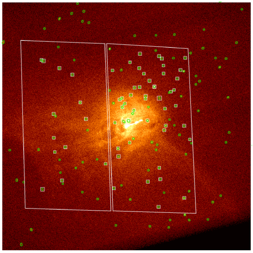
Figure 1.— Co-added Chandra/ACIS image of M87 with the ACS field of view overlaid (rhomboids). The X-ray point source detections are indicated by the green ellipses. White squares indicate the 60 X-ray sources that coincide with globular cluster candidates. North is up and East is to the left in this image, which measures $5^{\prime}\times 5^{\prime}$.

Two sources in particular merit attention (see Figure 2). The extraction ellipse of one X-ray source, CXOU J123047.1+122415 in Table 1, encloses three optical sources. In X-rays, the source is extended in a way that is consistent with being a blend of multiple sources. The centroid of the X-ray emission lies approximately halfway between the brightest optical detections, yet the three optical sources lie outside the nominal matching radius and so do not make it into the final catalog. We consider this to be a match when calculating the fraction of X-ray-optical matches by assuming that two of the GC matches hold an LMXB, but discard this source from the subsequent analysis. A second X-ray source (object CXOU J123046.7+122402 in Table 1) has two optical candidates within the matching radius. Given this ambiguity, we consider this to be a match for the purposes of estimating the overall frequency of LMXB-GC associations, but do not include this source in any other aspect of the analysis. All the candidate GCs in these two sources are metal-rich, so no ambiguity is introduced when calculating the frequencies for the metal-rich and metal-poor groups. Removing the two optical matches to CXOU J123046.7+122402 leaves 58 X-ray point source matches that will be used in the analysis.

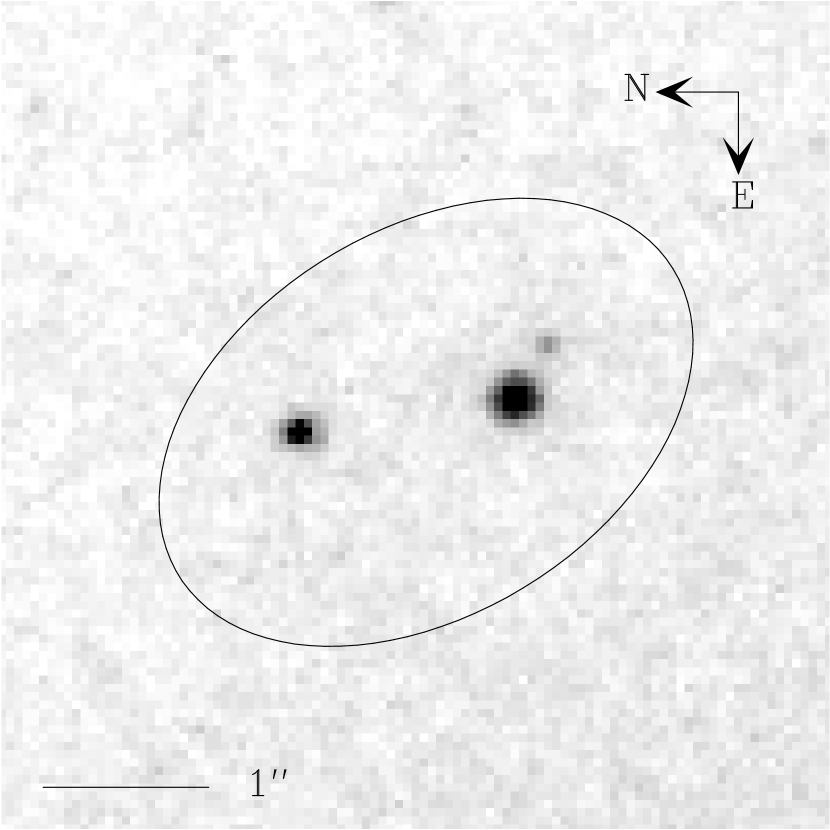
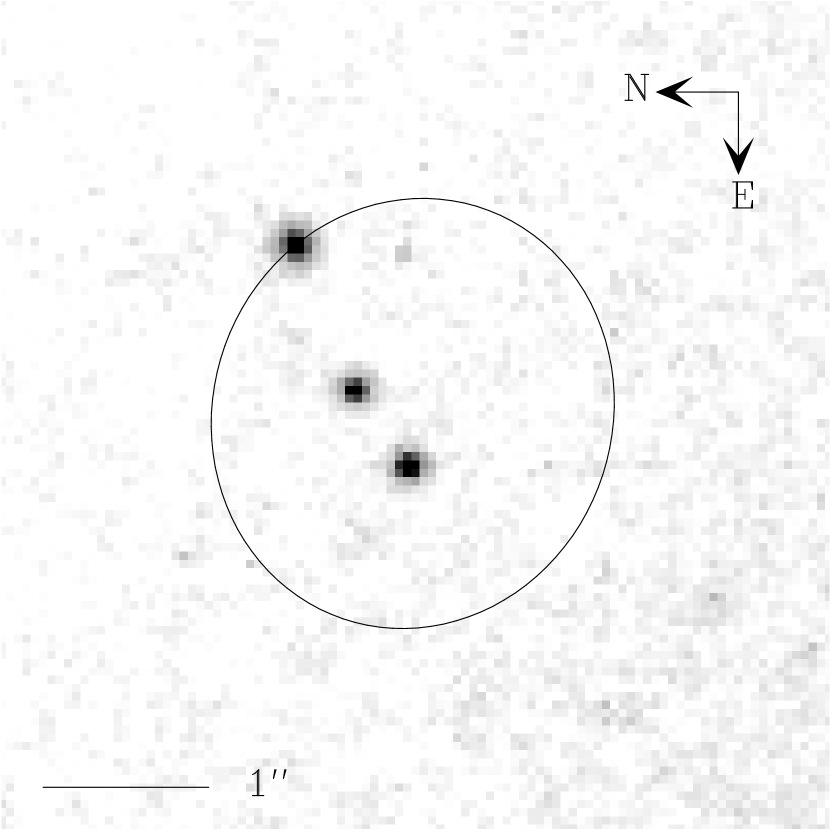
Figure 2.— (Left Panel) Portion of the ACS F850LP image in which the extraction region for the X-ray source CXOU J123047.1+122415 is marked by an ellipse. The X-ray source contains three GC candidates, none of which is within a matching radius of the X-ray emission centroid. (Right Panel) Portion of the ACS F850LP image in which the extraction region for the X-ray source CXOU 123046.7+122402 is marked by an ellipse. The X-ray source contains two GC candidates within one matching radius of its centroid.

Given the high GC surface density in M87, it is of interest to know the number of chance matches that might occur between the X-ray and optical datasets. We have estimated the number of such false matches by rotating the X-ray source coordinates about galaxy’s nucleus and calculating the total number of matches at each rotation angle. This exercise produced an average of four matches at each angle, so we conclude that the number of chance associations in our sample is small. According to the background source counts of Giacconi et al. (2001) and Mushotzky et al. (2000), we expect $\sim 2$ background sources within the ACS field of view. This is comparable to the number (2) of X-ray sources in our sample that match an optical source that is not a probable GC, so we believe that our sample has very little contamination from background sources and false matches.

2.4. Variability

We performed a simple search for variability among the 23 X-ray sources with $L_{X}>10^{38}$ erg s^-1 that coincide with a GC candidate. Using the positions from the combined observations, we measured the fluxes for the 2000 and 2002 datasets. The distribution of the flux differences, when divided by the expected uncertainty, reveals that seven sources show significant variability when compared with a normal distribution. Thus, the incidence of X-ray transients in the M87 GC/LMXB population appears roughly consistent with that of the Galaxy, where roughly half of all sources are known to exhibit time variability (e.g., Verbunt et al. 1995).

3. Spectral Analysis

All X-ray sources with galactocentric radii in the range $0.44R_{e}<r<2R_{e}$, were extracted and summed into a composite spectrum with the CIAO routine acisspec, which computes a weighted redistribution matrix file and ancillary response file (ARF) appropriate for point sources distributed over the ACIS detector. The ARF files were corrected for the degradation of the ACIS quantum efficiency using the CIAO tool apply_acisabs, which applies the ACISABS absorption profile (Chartas & Getman 2002) to the original ARF file. The extraction was performed independently for the 2000 and 2002 datasets, and the source spectra were regrouped so that each energy channel contained a minimum of $50$ photons, prior to background subtraction. In Figure 3, we show summed spectra from the 2002 dataset, for both the source regions ($i.e.,$ object plus background) and for the background regions alone.

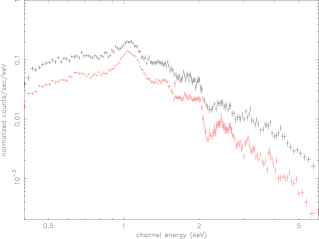
Figure 3.— Summed spectra for the background regions (red crosses) and for source regions prior to background subtraction (black crosses). The spectra are based entirely on data acquired in 2002.

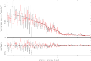
Figure 4.— Summed spectra for all X-ray sources, with the $2000$ data shown in black and the $2002$ data in red. The curves indicate the best-fit power-law model, with index $\kappa=1.64$, obtained by fitting simultaneously to both data sets. The lower panel shows the residuals from this best-fit model.

The composite, background-subtracted source spectra for the $2000$ and $2002$ datasets were fit simultaneously with XSPEC v11.2.0 (Arnaud 1996). The spectral energy distribution is assumed to have a single photon power-law behaviour $\propto E^{-\kappa}$. The Galactic hydrogen column density is held fixed at $N_{H}=2.5\times 10^{20}$ cm^-2 in the fit; channels with energy less then $0.7$ keV and greater than $4$ keV were excluded from the fit. The spectra, best-fit model and residuals are shown in Figure 4. The best-fit power-law exponent is $\kappa=1.64^{+0.047}_{-0.046}$ ($90\%$ confidence uncertainties), with a reduced chi-squared of $\chi^{2}_{\nu}=1.032$ with $218$ degrees of freedom. Irwin et al. (2003) analyzed the composite spectra of point sources within $3R_{e}$ for a sample of $15$ nearby galaxies, finding power-law exponents in the range $1.45\leq\kappa\leq 1.9$. Thus, our measured power-law exponent for the LMXBs in M87 is typical of those found in other nearby galaxies. This best-fit model is used to convert the observed counts to unabsorbed luminosities, $L_{X}$, over the range $0.3-10$ keV, assuming that all the sources are at the distance of M87. The resulting conversion factor is $1.4\times 10^{41}$ erg count^-1.

We examined the crude spectral properties of the resolved sources by calculating hardness ratios, which have the advantage of being measurable for even the faintest sources. Counts were calculated for three distinct energy bands: a soft ($0.3-1$ keV) band denoted by $S$, a medium band ($1-2$ keV) denoted by $M$, and a hard ($2-10$ keV) band denoted by $H$. Following Sarazin et al. (2000), the hardness ratios, H$31$ and H$21$, are taken to be

$$\begin{array}[]{rcl}H21&\equiv&(M-S)/(M+S)\\ H31&\equiv&(H-S)/(H+S)\\ \end{array}{}$$ (2)

The distribution of hardness ratios is shown in Figure 5. The sources occupy a diagonal swath in this plot, as is typical for LMXBs (Sarazin et al. 2000; Blanton et al. 2002; Irwin et al. 2003; Jeltema et al. 2003; Sivakoff et al. 2003). The mean location, at $(0.07,-0.21)$, is indicated by the cross. It is apparent from this figure that the most luminous sources appear to have the softest spectra, and a Wilcoxon test confirms this impression, giving probabilities of 6% and 0.6%, respectively, that the H$21$ and H$31$ values for sources with $L_{X}>5\times 10^{38}$ erg s^-1 share the same location. Although there are only six objects with $L_{X}>5\times 10^{38}$ erg s^-1, this result is consistent with that of Irwin et al. (2003), who noted that sources with $L_{X}>10^{39}$ erg s^-1 appear to be significantly softer. As they remark, this trend might be a reflection of inverse dependence between the emitted flux and spectral state exhibited by candidate black hole X-ray binaries in the Milky Way (e.g. Tanaka & Lewin 1995; Nowak 1995). Finally, we note that there are two sources in the upper right corner of Figure 5 in which both H$21$ and H$31$ are equal to $1.0$; given the hardness of these spectra, we suspect that these sources may be strongly absorbed AGN.

Figure 5.— Left: Hardness ratios, H21 and H31, for the full sample of 174 X-ray point sources. The size of the symbol for each source is proportional to its luminosity in the range 0.3–10 keV. The mean hardness ratios are $(\langle\mbox{H}21\rangle,\langle\mbox{H}31\rangle)=(0.07,-0.21)$, as indicated by the cross. Right: Hardness ratios, H21 and H31, for all sources with $L_{X}>1.5\times 10^{38}$ erg s^-1. Error bars give $1\sigma$ uncertainties in the ratios. The line shows predicted ratios for a power law with a hydrogen column density equal to $N_{H}=2.5\times 10^{20}$ cm^-2 (Stark et al. 1992); from top to bottom, the squares correspond to the predictions for power law exponents of 0, 1, 2 and 3.

4. Global Properties of the LMXB Population

We now turn our attention to the observed properties of the LMXB population as a whole ($i.e.$, spatial structure, luminosity function, and suitability as a distance indicator). Our ultimate aim is to understand the nature of the connection between LMXBs and GCs in M87, and to examine the broader implications for LMXB formation.

4.1. Radial and Azimuthal Structure

How does the radial distribution of LMXBs in M87 compare to that of its GCs and the underlying galaxy light? In comparing the various profiles, we restrict ourselves to X-ray point sources having $L_{X}>7\times 10^{37}$ ergs s^-1, and to GC candidates that do not fall within the regions masked during the X-ray point source detection procedure and having $z_{850}<22.8$ mag (a total of 867 objects) in order to guard against incompleteness effects. The heavy solid curve in Figure 6 shows the resulting cumulative distribution for the M87 GC system, calculated directly from the GC catalog described in §2.2.

In principle, it should also be possible to measure the profile of the galaxy itself from our ACS images. However, such an approach is undermined by the limited areal coverage of the ACS field and the fact that our ACS images, which are centered on the galaxy’s nucleus, provide limited constraints on the background surface brightness. Given these problems, we estimate the cumulative light distribution within the ACS field, ${\cal S}(r)$, by using the wide-field surface photometry of Caon, Capaccioli & Rampazzo (1990). For an annulus centered on the galaxy, the fractional area falling within the ACS field (excluding those regions masked during X-ray point source detection; see below) is $f_{a}(r)$. The cumulative distribution of galaxy light is then

$${\cal S}(r)=2\pi rf_{a}(r)10^{-0.4\mu(r)}\\$$ (3)

where $\mu(r)$ refers to the $B$-band surface brightness profile of Caon et al. (1990). Note that the implicit assumption of circular symmetry in Equation 3 is quite reasonable for M87, which has a luminosity-weighted mean ellipticity of $\langle\epsilon\rangle\sim 0.05$ inside $r\sim 2\farcm 75$ — the maximum galactocentric radius of our ACS field.

The thin solid curve in Figure 6 shows the cumulative profile of the galaxy light within the ACS field. A KS test confirms the well known result that the GC system of M87 has a shallower profile than the galaxy itself ($e.g.$, Grillmair et al. 1986; Harris 1986). Also shown in Figure 6 are the cumulative distributions for two LMXB subsamples: the dotted curve shows the distribution for those sources that are associated with GC candidates, while the dashed curve shows the distribution for the remaining X-ray sources. In both cases, we plot only those X-ray sources that fall within the ACS field. Since both samples are subject to the same selection effects, it is straightforward to compare these distributions directly. A two sample KS test accepts the hypothesis that they were drawn from the same parent sample.

Comparing the X-ray point source samples to the galaxy and GC profiles is more difficult. Our Chandra image reveals the inner $\sim 40^{\prime\prime}$ of M87 to have a remarkably complex structure in diffuse emission (Figure 1; see also Figure 1 of Young, Wilson & Mundell 2002 and Sparks et al. 2004). Because of this complexity, it was necessary to mask several problematic regions prior to object detection (see §2), limiting the region over which the various profiles can be compared. Perhaps as a consequence, a one-sample KS test accepts the hypothesis that both X-ray samples (i.e., those point sources with, and without, an associated GC candidate) were drawn from the same parent distribution as the galaxy light; moreover, a two-sample KS test accepts the hypothesis that they were drawn from the same parent distribution as the GC candidates. Stronger conclusions will require an expanded census of LMXBs but, given the brightness and complexity of the diffuse X-ray emission in the inner regions of M87, the requisite observations will prove extremely challenging.

We also explored the azimuthal distribution of the X-ray point source samples. In Figure 7 we show the cumulative distribution function for the X-ray point sources that are associated with a GC and those that are not. We also show the azimuthal distribution of the full GC sample (excluding regions that were masked in the X-ray point source detection). It is clear from the figure that the X-ray point sources associated with a GC follow the distribution of the full GC sample, and this is confirmed by a KS test. The X-ray point sources not associated with a GC seem somewhat deviant, but a KS test accepts the hypothesis that the sample was drawn from the same distribution as the full GC sample and the X-ray point sources associated with a GC with p-values of $p_{KS}=0.19$ and $p_{KS}=0.1$ respectively. This exercise reveals that the spatial distribution of X-ray point sources associated with a GC is representative of the full GC sample.

Figure 6.— Comparison for the radial distribution of galaxy light, globular clusters and LMXBs in M87. The heavy solid curve shows the cumulative distribution of 867 globular cluster candidates in the ACS field that are brighter than $z_{850}=22.8$. The thin solid curve shows distribution of galaxy light within our ACS field. The dotted curve shows the cumulative distribution of the 32 LMXBs in our ACS field that are brighter than $L_{X}=7\times 10^{37}$ erg s^-1 and coincide with a globular cluster candidate. The dashed curve show the cumulative distribution of the remaining sample of 15 LMXBs in the ACS field that are brighter than $L_{X}=7\times 10^{37}$ erg s^-1 but have no GC counterpart.

Figure 7.— Comparison for the azimuthal distribution of globular clusters and LMXBs in M87. The solid curve shows the cumulative distribution of all bona fide GC candidates. The dashed curve shows the cumulative distribution of the X-ray point sources that coincide with a GC and the dotted curve shows the cumulative distribution of the X-ray point dources that do not coincide with a GC.

4.2. Luminosity Function

Figure 8.— Observed $\log N(L_{X})$, where $N(L_{X})$ is the number of X-ray sources with $L>L_{X}$. The dashed line shows the distribution for all sources within the S3 chip; the sources within the ACS field and associated with globular cluster are represented by the solid line; those sources within the ACS field but not associated with a globular clusters are shown by the dot-dashed line. The smooth lines are the best-fit power-law luminosity distributions of the form $f\propto L_{X}^{-\gamma}$ with an upper cutoff such that $f=0$ for $L_{X}>10^{39}$ erg s^-1. For the full sample of all sources, and for the subsample of sources that not associated with a globular cluster, the background contamination has been removed as in Giacconi et al. (2001).

The luminosity function of LMXBs is of considerable interest, both as a rare constraint on the mass distribution of accreting sources in external galaxies, and as a potential distance indicator. Working with a sample of $\approx$ 80 LMXBs in NGC 4697, Sarazin et al. (2001) showed that their cumulative luminosity function was well described by a broken power-law, with a “break” at $L_{b}\approx 3.2\times 10^{38}$ ergs s^-1. Since this is close to the Eddington luminosity for spherical hydrogen accretion onto the surface of a $1.4M_{\odot}$ neutron star (e.g. Shapiro & Teukolsky 1983), Sarazin et al. (2001) drew attention to the possibility of using this feature as a standard candle in distance estimation. Indeed, the use of a characteristic luminosity in accreting neutron stars as a distance indicator dates to early studies of Galactic X-ray sources ($e.g.$, Margon & Ostriker 1973; van Paradijs 1978).

Figure 9.— Same as Figure 8, except for sources in M49 and NGC 4697. The dashed histogram shows the distribution of X-ray sources in M49 from the S3 chip of Kundu et al. (2002). The corresponding distribution for sources in NGC 4697 is given by the solid histogram (Sarazin et al. 2001). The dot-dashed histogram shows the distribution for sources in M49 that are associated with a globular cluster (Kundu et al. 2002). The smooth curves are best-fit power-law luminosity distributions of the form $f\propto L_{X}^{-\gamma}$ with an upper cutoff such that $f=0$ for $L_{X}>10^{39}$ erg s^-1. For the complete samples in both galaxies, the background contamination has been removed as in Giacconi et al. (2001).

4.2.1 Representation as a Broken Power-Law

In Figure 8, we show the cumulative luminosity function, $\log N(L_{X})$, of X-ray sources in M87. Here, $N(L_{X})$ is the number of objects with luminosities in excess of $L_{X}$. The dashed line shows this distribution for the complete sample of sources — a total of 174 objects. The two lower distributions show the distributions for those sources that fall within the ACS field: the solid line indicates those sources that coincide with a GC, while the dot-dashed line refers to sources with no associated GC. Aside from normalization, the three distributions appear remarkably similar; the abrupt flattening below $L_{X}\sim 4\times 10^{37}$ erg s^-1 is probably due to incompleteness. When fitting models to the luminosity functions, we have corrected for background contamination using the background counts of Giacconi et al. (2001) for the complete sample and the subsample of objects that are not associated with GCs.

To facilitate comparison with previous work, we have fitted these three distributions with broken power-laws of the form

$$\begin{array}[]{rcllll}N(L_{X})&\propto&L_{X}^{{\alpha}_{1}}&&{\rm for}&L_{X}<L_{b}\\ N(L_{X})&\propto&L_{X}^{{\alpha}_{2}}&&{\rm for}&L_{X}\geq L_{b}\\ \end{array}{}$$ (4)

To guard against incompleteness effects, we consider only those source brighter than $5\times 10^{37}$ erg s^-1. The resulting values for ${\alpha}_{1}$, ${\alpha}_{2}$ and $L_{B}$ are given in Table 2. Note that the break luminosities found here, $L_{B}\sim(2-3)\times 10^{38}$ erg s^-1, are similar to those found in other early-type galaxies ($e.g.$, Sarazin et al. 2001; Finoguenov & Jones 2001; Kundu et al. 2002). Although the observed luminosity distribution is well described by this particular choice of parameterization, the data do not require a broken power-law. As we now show, the data are equally well represented by a single power-law distribution with an upper cutoff in luminosity.

Figure 10.— The smooth solid line shows the expected behaviour of $\log N(>L)$ for a sample of size $100$ drawn from a distribution of luminosities given by $L^{-2}$ with an upper cut at $L=10^{39}$ erg s^-1. The rest of the lines show the observed behaviour of $5$ random realizations of size $100$ from that distribution.

4.2.2 Representation as a Truncated Power-Law

For each of the three samples of observed X-Ray luminosities, whose corresponding cumulative distributions are shown in Figure 8, we have fit single power-law distributions of the form $L_{X}^{\gamma}$ for $L_{min}<L_{X}<L_{max}$, taking $L_{max}=10^{39}$ erg s^-1 as the upper cutoff. As before, we adopt $L_{min}=5\times 10^{37}$ erg s^-1 to guard against incompleteness at the faint end. The corresponding best-fit cumulative distributions are shown as the smooth curves. In each case, a one-sample KS test reveals that the samples are consistent with their being drawn from a single power law with $\gamma\sim-2.1$. The best fit values for $\gamma$ are given in Table 2.

Is this true of the LMXB populations in other galaxies? In Figure 9, we show the cumulative luminosity functions of all LMXBs in NGC 4697 and M49 (using data from Sarazin et al. 2001 and Kundu et al. 2002, respectively). Maximum likelihood fits to both datasets reveals that they are consistent with having been drawn from a single power-law distribution with an upper cut at $L_{X}=10^{39}$ erg s^-1. The corresponding best-fit cumulative distributions, which have $\gamma=-1.63\pm 0.14$ (NGC 4697), $\gamma=-1.58\pm 0.12$ (M49, all X-ray point sources) and $\gamma=-1.64\pm 0.25$ (M49, X-ray sources associated with a GC), are given by smooth curves in Figure 9. As this exercise demonstrates, it is dangerous to draw conclusions about the underlying distribution, $f$, from the quantity $N(L_{X})$, particularly at the high-luminosity end, if $f$ is truncated above some value. Let us denote the cumulative distribution of $f$ by $F$, so that $\log N(L_{X})$ is equivalent modulo a constant to $\log(1-F)$. The slope $s$ of this function is given by $s=-f/(1-F)$. If $f=0$ for values of $L_{X}$ greater than $L_{max}$ then, as we approach $L_{max}$, we generically expect $\lim_{L\rightarrow L_{max}}s=-\infty$, producing a dip in the expected form of $\log(1-F)$. To give an example germane to the present discussion, let us assume that $f=L_{X}^{-2}$ with $f=0$ for $L_{X}>10^{39}$ erg s^-1. The corresponding distribution $N(L_{X})$ is shown as the smooth curve in Figure 10. For comparison, the histograms in this figure show five simulated datasets, each consisting of one hundred objects. Because the parent distribution is cut beyond a maximum $L_{X}$ some simulated datasets have an apparent break, even though the parent distribution has no characteristic scale to distinguish the two regimes.

Based on the evidence presented above, we conclude that there is no compelling evidence for two fundamentally different accretor populations in M87, M49 or NGC 4697, and that a single power-law distribution (truncated above $\sim 10^{39}$ erg s^-1) provides an adequate description of the LMXB populations in all three galaxies. Moreover, we have shown that the apparent “breaks” at $L_{X}\sim(1-4)\times 10^{38}$ erg s^-1 may be an artifact of this distribution. Our conclusions are in agreement with those of Sivakoff et al. (2003), who found that the luminosity distribution of LMXBs in NGC 4365 and NGC 4382 could be better modeled by a power law having an upper cutoff at $L_{X}\sim 10^{39}$ erg s^-1. This also appears to be the case in the Milky Way: Grimm, Gilfanov & Sunyaev (2001) find a truncated power law to be an excellent representation of the Galactic LMXB luminosity distribution.

In retrospect, the lack of a characteristic luminosity scale should perhaps come as no surprise since the Eddington luminosity, $L_{E}$, is usually computed under very particular assumptions: namely, spherical accretion of pure ionized hydrogen and Thomson scattering. This is clearly an idealized situation, and there are various ways in which an accreting neutron star can exceed this naive estimate: $e.g.$, unusual chemical abundance, formation of a super-critical disk, radiation in the form of relativistic jets and the presence of strong magnetic fields (see, $e.g.$, the discussion in Grimm et al. 2001 and references therein). Still another effect that would blur a characteristic scale is that the observed values of $L_{X}$ will be affected by disk obscuration and scattering. Irwin et al. (2003) find essentially no sources with $L_{X}>2\times 10^{39}$ erg s^-1 in their study of the LMXB populations of $15$ early-type galaxies, and our results are in line with theirs. Thus, it is likely that the luminosity function of LMXBs in most early-type galaxes is truncated at $L_{max}\sim(1-2)\times 10^{39}$ erg s^-1. This upper cutoff is probably not universal. Indeed, a significant number of very luminous sources ($L_{X}\mathrel{<\kern-10.00002pt\lower 3.87495pt\hbox{$\sim$}}10^{40}$ erg s^-1) have been observed in some early-type galaxies, such as NGC 720 (Jeltema et al. 2003). In NGC 720, the spatial distribution suggests that the more luminous sources could arise from a younger stellar population whose formation was perhaps triggered by a recent merger.

Figure 11.— Normalized, cumulative luminosity functions for LMXBs within the ACS field. The solid curve shows the distribution of LMXBs that are associated with a GC; LMXBs that are not associated with GCs are indicated by the dashed curve.

4.2.3 Environmental Dependence

Do the LMXBs in GCs share the same luminosity function as those which are not associated with GCs? There have been conflicting claims about such an environmental dependence in the LMXB luminosity function. In their study of NGC 1399, Angelini et al. (2001) found the LMXBs in GCs to be, on average, more luminous than those which are not associated with GCs. On the other hand, Kundu et al. (2002) found the two populations in M49 to have indistinguishable luminosity functions, and Sarazin et al. (2003) reached a similar conclusion based on their analysis of LMXBs in four early-type galaxies.

In Figure 11 we show the normalized, cumulative luminosity function for LMXBs within the ACS field. The solid curve shows the distribution of LMXBs that coincide with a GC, while the dashed curve shows those LMXBs that do not. The LMXBs associated with GCs are slightly brighter on average, with a mean luminosity of $\langle L_{X}\rangle=(1.4\pm 0.2)\times 10^{38}$ erg s^-1. The mean luminosity of LMXBs that are not associated with GCs is $\langle L_{X}\rangle=(1.1\pm 0.2)\times 10^{38}$ erg s^-1. The difference, however, is not significant at greater than $99\%$ confidence, as KS and Wilcoxon sum rank test accept the hypothesis that the data were drawn from the same distribution with p-values of $p_{KS}=0.1$ and $p_{wilcox}=0.1$, respectively. Thus, at least in the case of M87, we find no support for the claim that the LMXBs that are associated with GCs are significantly brighter than those which are not. These findings are consistent with the suggestion that essentially all LMXBs in early-type galaxies may have first formed in GCs (White, Sarazin & Kulkarni 2002) and were subsequently ejected or dispersed into the general field.

5. The Relation Between Low Mass X-Ray Binaries and Globular Clusters

5.1. The Efficiency of LMXB Formation

The most basic characterization of the probability that a GC harbors an LMXB is the overall probability, $p_{X}$, that a GC will host a LMXB candidate. Restricting ourselves to those sources in the ACS field of view, we find $p_{X}=0.036\pm 0.005$. This overall probability has been found to be in the range $2-4\%$ in a wide variety of galaxy types (see, e.g., Sarazin et al. 2003 and references therein), providing a very uniform characteristic of the connection between GCs and LMXBs in GCs. Another basic quantity is the fraction of X-ray point sources $f_{\rm X-GC}$ that reside in a GC; for M87 this is $f_{\rm X-GC}=0.62$. Observed values of $f_{\rm X-GC}$ vary substantially from galaxy to galaxy, from $\sim 0.2$ for sources in the central region of M31 (Primini, Forman & Jones 1993) to $\sim 0.7$ for NGC 1399 (Angelini et al. 2001), and it has been proposed that the available observations indicate a systematic increases along the Hubble sequence from late to early types (Sarazin et al. 2003). We now turn to consider the dependence of $p_{X}$ on various factors.

5.2. Dependence on Metallicity

In the Galaxy and M31, there is a tendency for LMXBs in GCs to appear preferentially in metal-rich GCs (Grindlay 1993; Bellazzini et al. 1995), but the limited samples sizes ($i.e.$, just 13 and 19 LMXBs, respectively, with $L_{X}>10^{36}$ erg s^-1; Verbunt 2001, White & Angelini 2001) have precluded definite conclusions. However, new observations have confirmed the trend with larger samples of LMXBs in NGC 1399 (Angelini et al. 2001), NGC 4472 (Kundu et al. 2002) and NGC 5128 (Minniti et al. 2004). Kundu et al. (2002) find that metal-rich GCs are, on average, $\sim 3$ times as likely to harbor LMXBs than their metal-poor counterparts.

In Figure 12, we show the ($g_{475}-z_{850}$) color distribution for the full sample of 1688 GCs in our ACS field, along with the corresponding distribution for the 58 GCs which coincide with an X-ray point source. It is apparent that LMXBs show a marked preference for metal-rich GCs, and this is confirmed with two different statistical tests: a two sample KS test rejects the hypothesis that the distributions were drawn from the same distribution with a p-value of $p_{KS}=3\times 10^{-4}$, while a Wilcoxon rank sum test rejects the hypothesis that the parent distributions have the same location with a p-value of $p_{wilcox}=2\times 10^{-4}$.

Figure 12.— Color histograms for the full sample of globular clusters (open bars) and for the sample of globular clusters which coincide with an X-ray point source (filled bars). The curve is a normal kernel density estimate of the color distribution, which we denote by $\hat{\Psi}(g_{475}-z_{850})$. The tickmarks show the colors of individual GCs associated with X-ray point sources.

To divide the color distribution into metal-rich and metal-poor subsamples, we use the KMM algorithm (Ashman, Bird & Zepf 1994). This algorithm performs the division based on an a posteriori likelihood using two Gaussians to model the color distribution. KMM gives a dividing color of ($g_{475}-z_{850}$) = 1.121, which we adopt as the division between the metal-rich and metal-poor subpopulations in M87. With the subpopulations defined in this way, we find a probability of $p_{X,MR}=5.1\pm 0.7$% that a given metal-rich cluster will contain a LMXB; this should be compared to the value of $p_{X,MP}=1.7\pm 0.5$% found for the metal-poor GCs. We conclude that metal-rich GCs are $3\pm 1$ times more likely to contain LMXBs than metal-poor GCs.

To get a quantitative estimate of the dependence of $p_{X}$ on metallicity, we model the color distribution of GCs which contain LMXBs as

$$\begin{array}[]{rcl}\psi&\sim&10^{\beta(g_{475}-z_{850})}\Psi,\\ \end{array}{}$$ (5)

where $\Psi$ is the color distribution for the full sample of GCs. To estimate $\Psi$, we use a kernel density estimate (Silverman 1986) which we denote by $\hat{\Psi}$, and determine $\beta$ via a maximum likelihood fit of the function

$$\begin{array}[]{rcl}\psi&\sim&10^{\beta(g_{475}-z_{850})}\hat{\Psi}\\ \end{array}{}$$ (6)

to the color distribution of the subsample of GCs that contain LMXBs. The result is $\beta=0.77\pm 0.22$, and the distribution predicted by equation (6) is compared to the observed one in Figure 13. To find the dependence of $p_{X}$ on metallicity, it would be best to use an empirical determination of the relation between $(g_{475}-z_{850})$ and [Fe/H], but unfortunately no such relation is available in the literature to the best of our knowledge. As a substitute, we use the models of Bruzual & Charlot (2003) to find the relation between $(g_{475}-z_{850})$ and [Fe/H]. Using the data listed in Table 3, we find a best-fit linear relation of $(g_{475}-z_{850})\sim(0.38\pm 0.05)\mbox{[Fe/H]}+(1.62\pm 0.06)$, with an rms scatter of roughly 0.1 mag. Using this relation, we find

$$\begin{array}[]{rcl}\psi&\sim&10^{(0.32\pm 0.10)\mbox{{\scriptsize[Fe/H]}}}\hat{\Psi}\\ &\sim&(Z/Z_{\odot})^{(0.32\pm 0.10)}\hat{\Psi}\\ \end{array}{}$$ (7)

We also reanalyzed the metallicity dependence of LMXBs in the GC system of M49, using the ($V-I$) colors presented in Maccarone et al. (2002). Fitting a model of the form of equation (6), we find $\beta_{VI}=1.2\pm 0.5$. The empirical color-metallicity relation of Barmby et al. (2000) then gives

$$\begin{array}[]{rcl}\psi_{VI}&\sim&10^{(0.19\pm 0.08)\mbox{{\scriptsize[Fe/H]}}}\hat{\Psi}_{VI}\\ &\sim&(Z/Z_{\odot})^{(0.19\pm 0.08)}\hat{\Psi}_{VI}\\ \end{array}{}$$ (8)

consistent with our findings for M87. The color distribution for the M49 data, along with the best-fit model, is shown in Figure 14.

Figure 13.— Histogram of $(g_{475}-z_{850})$ colors for 58 globular cluster in M87 which coincide with an X-ray point source. The curve shows a model color distribution of the form $\psi\sim 10^{\beta(g_{475}-z_{850})}\hat{\Psi}$, with $\beta=0.77$ (see text for details). The tickmarks show the colors of individual objects.

Figure 14.— Histogram of $(V-I)$ colors for globular clusters in M49 that coincide with an X-ray point source, according to Maccarone et al. (2002). The curve shows a model color distribution of the form $\psi_{VI}\sim 10^{\beta_{VI}(V-I)}\hat{\Psi}_{VI}$, with $\beta_{VI}=1.2$ (see text for details). The tickmarks show the colors of individual objects.

5.3. Dependence on Luminosity

In addition to metallicity, luminosity plays an important role in determining whether a given GC will contain a LMXB (in the sense that LMXBs reside preferentially in the most luminous clusters). This has been observed to be the case in NGC 1399 (Angelini et al. 2001), M49 (Kundu et al. 2002), four early-type galaxies analyzed in Sarazin et al. (2003) and NGC 5128 (Minniti et al. 2004). Given that our ACS observations of M87 define the deepest, most complete sample of GCs yet assembled for any galaxy, we now examine the dependence of $p_{X}$ on luminosity in M87.

In Figure 15, we show the $z_{850}$-band luminosity function for the full sample of 1688 GCs within the ACS field of view (open histogram), along with the corresponding luminosity function for those 58 GCs which coincide with an X-ray point source (filled histogram). It is clear that, in agreement with previous findings, the LMXBs are associated preferentially with the brighter GCs. A two sample KS test rejects the hypothesis that the two datasets were drawn from the same parent distribution and a Wilcoxon rank sum test rejects the hypothesis that the parent distributions share the same location; the respective p-values are $p_{KS}=7\times 10^{-11}$ and $p_{wilcox}=7\times 10^{-14}$.

Figure 15.— $z_{850}$-band luminosity function for the full sample globular cluster candidates (empty bars) and for those candidates that coincide with an X-ray point source (filled bars). The curve is a normal kernel density estimate of the luminosity function, which we denote by $\hat{\Phi}(m)$. The tickmarks show the magnitudes of individual GCs associated with X-ray point sources.

Both Kundu et al. (2002) and Sarazin et al. (2003) argue that the data are consistent with the probability per unit luminosity being constant. To represent the luminosity function of those GCs that coincide with LMXBs, $\phi(m)$, we will adopt a probability density of the form

$$\begin{array}[]{rcl}\phi(m)&\sim&L^{\alpha}\Phi(m)\\ &\sim&10^{-0.4\alpha m}\Phi(m)\\ \end{array}{}$$ (9)

where $\Phi(m)$ is the distribution of GC magnitudes. At this point, we could model $\Phi(m)$ parametrically (e.g., by using a Gaussian and taking care to model the effects of incompleteness). However, we prefer to approximate $\Phi(m)$ using a normal kernel density estimate (Silverman 1986) since this approach does not require us to make any assumptions about the true parent distribution, while at the same time, the effects of incompleteness are taken into account.

Denoting the kernel density estimate by $\hat{\Phi}(m)$, we determine the parameter $\alpha$ via a maximum likelihood fit of the function $10^{-0.4\alpha m}\hat{\Phi}(m)$ to the observed distribution, $\phi(m)$. The result is $\alpha=0.89\pm 0.12$, which is consistent with the results of Sarazin et al. (2003), who found that the luminosity function of GCs with associated LMXBs was consistent with the form $\phi(m)\sim L\Phi(m)$. In Figure 16, we show the luminosity function of GCs with an associated LMXB, along with the best-fit LMXB luminosity functions $\phi\sim L^{0.89}\hat{\Phi}(m)$ (solid curve) and $\phi\sim L\hat{\Phi}(m)$ (dashed curve).

Figure 16.— $z_{850}$ band luminosity function for globular cluster candidates with an associated X-ray point source. The solid and dashed curves are model distributions of the form $\psi\sim L^{\alpha}\hat{\phi}$, with $\alpha=0.89$ and $\alpha=1$, respectively. The tickmarks show the magnitudes of individual objects.

5.4. Dependence on Encounter Rates

For the first time for a galaxy outside the Local Group, we are able to examine possible variations of $p_{X}$ with GC structural parameters. The number of LMXBs is expected to depend on these parameters since the binaries responsible for the X-ray emission are likely to have a dynamical origin. That is to say, compact binaries in which one of the components is a neutron star are probably not primordial in nature, but have likely formed as a result of the tidal capture of neutron star, or by exchange interactions with pre-existing binaries (Verbunt 2002).

The encounter rates, $\Gamma$, for both tidal capture and exchange interactions satisfy

$$\Gamma\propto\frac{\rho_{0}^{2}r_{c}^{3}}{v}$$ (10)

where $\rho_{0}$ is the central mass density of the GC, $r_{c}$ is the core radius and $v$ is the relative velocity of the encounter (Hut & Verbunt 1983). An estimate of $v$ can be obtained from the velocity dispersion of the cluster, which in turn is related to the central density and core radius via the virial theorem, $\sigma\propto r_{c}\sqrt{\rho_{0}}$. To be sure, other factors will affect the encounter rates for a given cluster, such as the rate at which binaries formed by these mechanisms are subsequently disrupted, the mass function in the cluster core, the binary fraction, and the period distribution of the binaries (Verbunt 2002). In this section, however, we concentrate on the explicit dependence of $\Gamma$ on structural parameters; the role of other factors, which may themselves depend on metallicity and structural parameters, will be examined in §5.5. In the absence of more detailed information, we will first test the simple scenario in which $p_{X}$ is proportional to

$$\Gamma\equiv\rho_{0}^{1.5}r_{c}^{2}.$$ (11)

To compute $\Gamma$, we use the relations between core radius and half-light radius, $\log{\cal R}(c)\equiv\log(r_{h}/r_{c})$, and between the dimensionless luminosity, $\log{\cal L}(c)\equiv\log(L/j_{0}r_{c}^{3})$, and King concentration parameter, $c\equiv\log(r_{t}/r_{c})$, which are given in Appendix B of McLaughlin (2000). Here, $j_{0}$ is the central luminosity density, $r_{h}$ is the half-light radius, $r_{c}$ is the core radius, $r_{t}$ is the tidal radius and $L$ is the cluster’s $V$-band luminosity. Explicitly, if $m$ is the $z_{850}$-band magnitude, $DM=31.03$ the distance modulus of M87 (Tonry et al. 2001), $M_{V,\odot}=4.84$ the absolute V-band magnitude of the Sun (Vandenberg & Bell 1985), $j_{0}$ the central $V$-band luminosity density, and $\Upsilon_{V}$ the $V$-band mass-to-light ratio, then the central mass density, in units of $M_{\odot}$ pc^-3, is given by the expression

$$\rho_{0}=\Upsilon_{V}j_{0}=\Upsilon_{V}\frac{10^{-0.4(m-DM-M_{V,\odot}+c_{V})}}{(r_{h}/{\cal{R}})^{3}{\cal{L}}}$$ (12)

where the core radius is given by $r_{c}=r_{h}/{\cal{R}}$ and $c_{V}$ is the color term needed to convert from $z_{850}$-band to $V$-band luminosity. The $V$-band mass-to-light ratios of Galactic GCs are consistent with a constant value of $\Upsilon_{V}=1.45$ in solar units (McLaughlin 2000), which we henceforth adopt for the M87 GCs. In general, the color term $c_{V}$ is ill-defined as it will depend on age and metallicity. We assume that the bulk of the GCs in M87 are old and coeval, as is suggested by spectroscopic and photometric age measurements (Cohen, Blakeslee & Ryzhov 1998; Jordán et al. 2002; Kissler-Patig et al. 2002). Assuming a mean age of $13$ Gyr (Cohen et al. 1998), we obtain the relation between ($g_{475}-z_{850}$) and ($V-z_{850}$) using the population synthesis models of Bruzual & Charlot (2003). For each ($g_{475}-z_{850}$) color, we linearly interpolate (or extrapolate, if necessary) to find the corresponding ($V-z_{850}$) at each of the metallicities in the Bruzual & Charlot (2003) models. The data used to define the color-color relation are listed in Table 3.

Figure 17.— Distribution of $(g_{475}-z_{850})$ color as a function of encounter rate, $\Gamma\equiv\rho_{0}^{1.5}r_{c}^{2}$, for the full sample of 1688 globular clusters (small crosses). Large circles indicate the 58 globular clusters which contain a LMXB.

For the full sample of 1688 GCs, we find a mean encounter rate of $\langle\log\Gamma\rangle=5.8\pm 0.02$. For comparison, the mean encounter rate for the subsample of 58 GCs which coincide with a LMXB is $\langle\log\Gamma\rangle=6.73\pm 0.09$. A two sample KS test rejects the hypothesis that the distribution of $\Gamma$ parameters for these two samples arise from the same parent distribution and a Wilcoxon rank sum test rejects the hypothesis that they have the same location; the respective p-values are $p_{KS}=3\times 10^{-11}$ and $p_{wilcox}=3\times 5^{-15}$. This constitutes the strongest evidence to date that encounter rates play a key role in determining $p_{X}$.

This finding is also consistent with the results of Pooley et al. (2003) and Heinke et al. (2003). Pooley et al. (2003) find that $\Gamma$ is the main factor in determining the number of close X-ray binaries in Galactic GCs. Specifically, they find $p_{X}\propto\Gamma$ after restricting their analysis to the subset of GCs which contain bonafide LMXBs (see also Verbunt & Hut 1987), although their conclusions are hampered by the limited sample size. Heinke et al. (2003) find that the population of quiescent LMXBs in Galactic GCs is consistent with their dynamical origin as indicated by $\Gamma$. In M31, Bellazzini et al. (1995) have shown that the central density of GCs which host LMXBs is higher than the mean central density of M31 GCs, which also points to the importance of encounter rates in determining the presence of LMXBs in GCs. Taken together, there seems to be little doubt that exchange interactions and tidal captures in GCs are largely responsible for the production of LMXBs.

In Figure 17, we plot the measured values of $\Gamma$ against ($g_{475}-z_{850}$) color for the full sample of GCs (small symbols), along with the subsample of GCs which contain LMXBs (large symbols). There is a clear tendency for the latter GCs to have higher than average encounter rates, and it is apparent that no obvious correlation exists between $\Gamma$ and GC color (recall from § 5.2 that metallicity is an important factor in determining $p_{X}$). Since the encounter rate and metallicity are uncorrelated, we can assume they are independent so that $p_{X}\propto p_{1}(\Gamma)p_{2}(\mbox{[Fe/H]})$.

In §5.3, we showed that there is a strong correlation between $p_{X}$ and GC luminosity. In Figure 18, we plot $\Gamma$ versus $z_{850}$-band magnitude for the full sample pf GCs (small symbols), as well as for the those GCs which are associated with a LMXB (large symbols). There is a clear tendency for $\Gamma$ to increase with increasing luminosity, which raises the possibility that the trend discussed in §5.3 is a consequence of a more fundamental correlation between $\Gamma$ and luminosity. In fact, we can predict the luminosity distribution of GCs which contain LMXBs, $\phi(m)$, under the assumption that $p_{X}\propto\Gamma$. Since there is no correlation between luminosity and color in the M87 GC system (Whitmore et al. 1995; Harris, Harris & McLaughlin 1998), we can safely ignore the metallicity dependence of $p_{X}$ when making this prediction. To find the behaviour of $\Gamma$ as a function of $z_{850}$-band magnitude, $m$, we fit a cubic smoothing spline to the data in Figure 18. The resulting relation, $\Gamma(m)$, is shown in Figure 18 as the smooth curve. Using a kernel density estimate, $\hat{\Phi}(m)$, of the magnitude distribution for the full sample of GCs, the predicted distribution for the subsample of GCs that contain LMXBs should then satisfy $\phi(m)\sim\Gamma(m)\hat{\Phi}(m)$.

This predicted distribution is shown as the dotted line in Figure 19. We stress that no fitting has been done in making this comparison; the only assumption is that $p_{X}\propto\Gamma$. The predicted distribution is in reasonable agreement with the observed distribution, although it seems to underpredict somewhat the number of faint GCs. A one-sample KS test gives $p_{KS}=0.07$, which does not allow us to reject the hypothesis that the observed distribution is explained by the assumption $p_{X}\propto\Gamma$ with better than $99\%$ confidence.

Rather than assume $p_{X}\propto\Gamma$, we now consider the dependence of $p_{X}$ on a more general quantity, $\Gamma_{\alpha}$, which satisfies

$$\Gamma_{\alpha}\propto\rho_{0}^{\alpha}r_{c}^{2}$$ (13)

where $\alpha$ is a free parameter that is determined by fitting to the observed magnitude distribution of those GCs which contain LMXBs. Such a form for the encounter rate has been considered previously by Johnston, Kulkarni & Phinney (1992), who find $\alpha\sim 1.3$ from an analysis of pulsars in Galactic GCs, and by Johnston & Verbunt (1996) who also find $\alpha\sim 1.3$ from an analysis of low-luminosity X-ray sources in Galactic GCs. By adding this additional parameter, we are able to account for possible variations in other factors which may influence the probability of forming LMXBs, such as variations in the initial mass function (IMF) or systematic variations in the relative importance of tidal captures and binary-neutron star exchanges (cf. Grindlay 1996) . We would like $\Gamma_{\alpha}$ to share with $\Gamma$ the property of being uncorrelated with $(g_{475}-z_{850})$ so as to be able to consider them independent variables and thus to write $p_{X}=p_{1}(\Gamma_{\alpha})p_{2}(\mbox{[Fe/H]})$. We therefore define $\Gamma_{\alpha}$ as

$$\Gamma_{\alpha}\equiv\rho_{0}^{\alpha}r_{c}^{2}10^{(0.46-\alpha 0.33)(g_{475}-z_{850})},$$ (14)

where we have made use of the fact that $r_{c}^{2}\sim 10^{(-0.46\pm 0.06)(g_{475}-z_{850})}$ and $\rho_{0}\sim 10^{(0.33\pm 0.09)(g_{475}-z_{850})}$. The latter expressions are best-fit relations obtained from our data. To determine $\alpha$, we fit via maximum likelihood a function of the form $\phi\sim\Gamma_{\alpha}\hat{\Phi}(m)$ to the observed distribution, where, as before, $\hat{\Phi}$ is a normal kernel density estimate of the GCs magnitude distribution and the behaviour of $\rho_{0}$ and $r_{c}^{2}$ as a function of magnitude has been obtained with smoothing splines. While formally it is more sound to include the color factor, we note that it has a negligible effect on the derived $\alpha$ since there is no color-luminosity correlation among M87 GCs. The best-fit value is $\alpha=1.08\pm 0.12$, the resulting $\phi$ (the solid curve in Figure 19) shows very good agreement with the data .

To summarize, we have shown that the encounter-rate based quantity $\Gamma$ is an important factor in determining $p_{X}$. Moreover, we have shown that $\Gamma$, and the more general parameter $\Gamma_{\alpha}$, can account quantitatively for the observed magnitude distribution of GCs containing LMXBs. Whether one wishes to assign a more fundamental role to $\Gamma$ or $\Gamma_{\alpha}$, rather than luminosity, becomes to some extent a matter of taste. However, we believe that it is more correct to view $p_{X}$ as being dependent on encounter-rate based quantities, as there are strong theoretical arguments to support this interpretation. This is not true of the alternative view that $p_{X}$ depends fundamentally on cluster luminosity (i.e., more stars do not necessarily imply a more favorable environment for the production of compact binaries).

Figure 18.— Plot of $z_{850}$-band magnitude versus $\log\Gamma$ for all globular clusters (small crosses). Large circles indicate those clusters that coincide with a LMXB. The curve shows a smoothing spline fit to the full dataset.

Figure 19.— $z_{850}$-band luminosity function for globular clusters with an associated LMXB. The solid curve is a model distribution of the form $\phi\sim\Gamma_{\alpha=1.08}\hat{\Phi}$, while the dashed curve shows a model of the form $\phi\sim\Gamma\hat{\Phi}$. The tickmarks show the magnitudes of individual objects.

5.5. Implications of the Derived Form for $p_{X}$

Combining the results of the previous sections, our estimate for $p_{X}$ is

$$\begin{array}[]{rcl}p_{X}&\sim&\Gamma_{\alpha=1.08}10^{\beta(g_{475}-z_{850})}\\ &\sim&\rho_{0}^{1.08}r_{c}^{2}10^{0.87(g_{475}-z_{850})}\\ &\sim&\rho_{0}^{1.08}r_{c}^{2}(Z/Z_{\odot})^{0.33}.\\ \end{array}$$ (15)

Our goal in this section is to use this empirical relation to: (1) test the validity of the various physical mechanisms which have been proposed for the production of LMXBs in dense stellar environments; and (2) understand the origin of the observed metallicity dependence.

There have been some theoretical suggestions as to why Galactic LMXBs might be more common in metal-rich GCs. For instance, Grindlay (1987) noted that, if the IMF depends on metallicity in such a way as to get flatter with increasing metallicity, then this would provide a larger population of massive stars (the progenitors of neutron stars in the LMXBs). A second, rather different, possibility is the suggestion by Bellazzini et al. (1995) that stars of higher metallicity will have larger radii and higher masses, thereby leading to enhancements in the tidal capture rates in metal-rich environments. Bellazzini et al. (1995) also note that such stars will more easily fill their Roche Lobes, further enhancing the number of LMXBs in metal-rich GCs. Recently, Maccarone et al. (2004) have suggested that irradiation induced winds on the donor star can explain the observed trend with metallicity. We now examine these suggestions in detail.

5.5.1 Dependence of the Number of Compact Stars per Unit Initial Mass on Metallicity

Let us denote the number of neutron stars produced per unit initial mass by $\nu$, the fraction of these neutron stars that are retained by the cluster by $f$, and the total encounter rate (including both tidal captures and binary exchanges) by $\Gamma_{t}$. Then

$$\Gamma_{t}\propto f\nu\rho_{0}^{1.5}r_{c}^{2}(\sigma_{2}+\sigma_{3})T$$ (16)

where $\rho_{0}$ is the central mass density, $r_{c}$ is the core radius, $T$ is the timescale over which the process lasts, and $\sigma_{2}$ and $\sigma_{3}$ are the respective cross sections for tidal capture (two-body) and binary exchange (three-body) interactions (Johnston et al. 1992). Note that the cross-section for tidal capture scales with the radius, $R$, of the capturing star, while the binary exchange cross section scales with the semi-major axis, $a$, of the binary: $i.e.$, $\sigma_{2}\propto R$ and $\sigma_{3}\propto a$.

Let us first consider possible metallicity-dependent variations in the fraction of neutron stars that are retained in GCs. Johnston et al. (1992) show that, for Galactic GCs, $f$ varies by a factor of $3\mathrel{<\kern-10.00002pt\lower 3.87495pt\hbox{$\sim$}}f\mathrel{<\kern-10.00002pt\lower 3.87495pt\hbox{$\sim$}}5$, with the precise value depending on the assumed velocity distribution of newborn neutron stars. For the same sample of GCs, however, $\rho_{0}$ varies by more than two orders of magnitude. Therefore, even though more massive GCs should certainly retain a greater fraction of their neutron stars, the net effect on $\Gamma_{t}$ is much smaller than that coming from the increase in the central density $\rho_{0}$, and we thus neglect it. The inclusion of this effect would steepen the dependence of $\Gamma_{t}$ on $\rho_{0}$. Note also that for GCs metallicity does not correlate with mass ($e.g.$, McLaughlin & Pudritz 1996), so we expect $f$ to be independent of metallicity.

We follow usual practice in assuming that $T$ is the same for the metal-rich and metal-poor subpopulations. Since the two subpopulations in M87 are observed to be roughly coeval (Cohen, Blakeslee & Ryzhov 1998; Jordán et al. 2002; Kissler-Patig et al. 2002), this assumption is reasonable, at least on average, although perhaps questionable for individual clusters which may have suffered substantial dynamical evolution.

Discounting a strong metallicity dependence in $\sigma_{2}$ or $\sigma_{3}$ (see § 5.5.2), we are left with the result that the best candidate in $\Gamma_{t}$ to contain the metallicity dependence of $p_{X}$ is $\nu$. Thus, we find that the observations point to a variation in the number of neutron stars formed per unit mass with GC metallicity, in the sense that more metal-rich GCs produce more neutron stars per unit initial mass. Such a variation could be a consequence of variations in the IMF, as proposed by Grindlay (1987). But even for similar IMFs, metallicity will have important effect on stellar evolution which will affect the number of neutron stars and black holes per unit mass. For instance, mass loss is thought to be greater for metal-rich stars and this will have a direct influence in the post-main-sequence evolution of high mass stars (Heger et al. 2003). Thus, the metallicity dependence in $\nu$ can plausibly arise through more than one process. Below we investigate on the possibility of IMF variations as the cause for the metallicity dependence, but it should be stressed that the result that $\nu$ should be higher for GCs of higher metallicity is independent of the IMF being the cause of this dependence.

In describing the IMF we will use a power law description, with the number of stars with masses between $m$ and $m+dm$ given by $N(m)\propto m^{-x}dm$ (where Salpeter is $x=2.35$). This form is believed to be a good description of the Galactic IMF only for stars with masses $M\mathrel{>\kern-10.00002pt\lower 3.87495pt\hbox{$\sim$}}1M_{\odot}$; for lower masses a lognormal distribution appears to be a better description of the IMF (Chabrier 2003). Nevertheless, we use the power-law form for simplicity and to allow direct comparison with previous work. Our main focus below is the effect of IMF variations in the relative number massive stars that end their evolution as neutron stars. Using a power law description this translates into a change in the IMF slope (assuming that all stars more massive than a certain value end up as neutron stars regardless of other factors).

If variations in $\nu$ alone are responsible for the observed scaling of $p_{X}$ with metallicity through IMF variations, then we can determine the behaviour that is required to produce the observed $p_{X}$. If all stars with $m>m_{NS}$ evolve to form neutron stars, then assuming that the minimum and maximum stellar masses are $m_{l}$ and $m_{u}$, respectively, the number of neutron stars per unit mass, $\nu$, is given by (for $x\neq 1,2$)

$$\nu(x)=\frac{x-2}{x-1}\bigg{[}\frac{m_{u}^{1-x}-m_{NS}^{1-x}}{m_{u}^{2-x}-m_{l}^{2-x}}\bigg{]}.$$ (17)

We parameterize the dependence of the IMF on metallicity by assuming $x$ depends linearly on [Fe/H], so $dx/d\mbox{[Fe/H]}\equiv A$. We restrict the metallicity range to $-2<\mbox{[Fe/H]}<0$, which includes the vast majority of M87 GCs (Cohen et al. 1998). We assign $x=-2.35$ to [Fe/H]$=-1.0$, assume $m_{l}=0.08\,M_{\odot}$, $m_{u}=100\,M_{\odot}$, $m_{NS}=8\,M_{\odot}$, and then find $A$ by minimizing the quantity

$$Q=\int_{-2}^{0}(C\nu(\zeta,A)-D10^{0.33\zeta})^{2}\,d\zeta,$$ (18)

where $C$ and $D$ are normalization constants. The result of the minimization gives $A=-0.3\pm 0.13$ dex^-1, where the quoted uncertainty corresponds to the uncertainty in the metallicity dependence of $p_{X}$. Thus, the inferred metallicity dependence is fairly weak. This result is in good agreement with the analysis of LMXBs in the Galactic and M31 GC systems presented by Bellazzini et al. (1995), who find that $A\sim-0.4$ dex^-1 is necessary to be consistent with the ratio of LMXBs in metal-rich and metal-poor clusters.

In their multivariate analysis of the Galactic GC system, Djorgovski et al. (1993) found that the intrinsic dependence of $x$ on metallicity among Galactic GCs — after removing the contribution of other important factors such as galactocentric distance, $R_{GC}$, and the distance from the Galactic plane, $Z_{GP}$ — is $A\approx-0.5$ dex^-1. Strictly speaking, these scaling relations are based on the present-day mass function in GCs, but it is reasonable to assume that this value of $A$ reflects the dependence of the initial mass function on metallicity, as dynamical effects like cluster evaporation might be implicitly accounted for by the dependence on $R_{gc}$ and $Z_{gp}$ (Stiavelli et al. 1991). In any event, it is remarkable that our estimate for the required metallicity dependence of IMF slope is in good agreement with that found in the Galaxy. Thus, a difference in the IMF between the chemically distinct GC subpopulations remains a viable explanation for the observed metallicity dependence of $p_{X}$.

5.5.2 Dependence of Stellar Radii on Metallicity

Bellazzini et al. (1995) argue that there is a second factor that can, in principle, increase $p_{X}$ for metal rich GCs. According to these investigators, stars in high-metallicity GCs will have larger radii and masses than those in metal-poor GCs, leading to an enhancement in their tidal capture cross sections. To estimate the magnitude of the effect, Bellazzini et al. use the expression for the tidal capture rate, $\Gamma^{TC}$, given in Lee & Ostriker (1986):

$$\Gamma^{TC}\propto R^{2-\tau}M^{\tau}N.$$ (19)

Here $R$ is the radius of the capturing star, $M$ is its mass, $N$ the total number of such stars, and the power-law index, $\tau=1.07$, is appropriate for our case (Lee & Ostriker 1986). Using the stellar evolution models of Vandenberg & Bell (1985), Bellazzini et al. (1995) find a ratio of capture rates for metal-rich and metal-poor stars of $\eta\equiv\Gamma^{TC}_{MR}/\Gamma^{TC}_{MP}\sim 2.2$. The enhancement is therefore comparable to the factor of three difference in $p_{X}$ which we find for the two GC subpopulations in M87.

However, the precise route to this ratio is not spelled out, and we were unable to reproduce their result. To estimate $\eta$, we use isochrones of the Bergbush & Vandenberg (1992), adopt [Fe/H]$=-0.47$ and [Fe/H]=$-1.82$ for the metal-rich and metal-poor GC subpopulations, respectively, and assume an age of $13$ Gyr for both subpopulations. From equation 19, we find $\eta\sim 2$ if we compare two stars at the tip of the red giant branch, but this hardly constitutes a representative estimate for the whole population. The latter comparison might be misleading though, as the changes in the structure of a star as it ascends the red giant branch make the application of the cross section of Lee & Ostriker (1986) dubious. McMillan, Taam & McDermott (1990) find that the critical impact parameter in units of the star radius is smaller for red giant stars than main sequence stars, and that it decreases as a star evolves through the red giant branch. In what follows we will neglect this effect, but note that inclusion of it would further reduce the magnitude of the effect advocated by Bellazini et al. (1995).

A representative estimate of $\Gamma^{TC}$ may be obtained as follows. Assuming that the IMF is described by a power law, $N(m)=m^{-x}dm$, we set

$$\Gamma^{TC}=\frac{\sum_{i}R_{i}^{2-\tau}M_{i}^{\tau}m_{i}^{-x}\Delta m_{i}}{\sum_{i}m_{i}^{-x}\Delta m_{i}}$$ (20)

where $i$ runs over all tabulated masses. We thus weight the tidal capture rates by the expected number of stars at each mass. Using this approach, we find $\eta\sim 1.1$, with a modest dependence on the assumed value of $x$. Thus, given similar IMFs, this effect enhances the tidal capture probability of the metal-rich GCs by a negligible amount.

A difference in IMF slope between the two GC subpopulations (see §5.5.1) has some effect on the estimated ratio. In this case, a correction factor — similar in form to the one in equation 17 with $m_{NS}$ replaced by $m_{l}$, and $m_{u}$ and $m_{l}$ set to the maximum and minimum masses in the isochrones — must be included to account for the fact that the number of stars per unit mass depends on $x$. Denoting such factor by $n(x)$, the ratio is then

$$\eta=\frac{n(x_{MR})\Gamma^{TC}_{MR}(x_{MR})}{n(x_{MP})\Gamma^{TC}_{MP}(x_{MP})}.$$ (21)

Taking $x=2.35$ for the metal-poor population and $x=1.7$ for the metal-rich (appropriate for the metallicity dependence of IMF slope in Galactic GCs, according to Djorgovski et al. 1993), we find $\eta\sim 1.3$. If instead we set $x=1.35$ for the metal-rich IMF, then the ratio increases to $\eta\sim 1.5$. Thus, even under rather extreme assumptions for the metallicity dependence of IMF slope, the enhancement is insufficient to explain the observed factor of three difference in $p_{X}$. And, in any event, such a difference in $x$ would result in a much larger enhancement in $p_{X}$ through the increase in the relative numbers of neutron star progenitors (i.e., see §5.5.1).

To summarize, we suggest that if the form of $p_{X}$ is determined solely by dynamical processes, an increase in relative number of high-mass stars forming in metal-rich environments remains the only viable explanation for the observed metallicity dependence of $p_{X}$, although a full treatment of the problem should take into account the modest variations in tidal capture rates expected for stars of differing metallicity.

5.5.3 Irradiation Induced Stellar Winds

The discussion so far has assumed that $Z$ has no effect on intrinsic properties of LMXBs, such as their typical lifetimes and luminosities, which might also produce the observed dependence of $p_{X}$ on metallicity. Recently, Maccarone et al. (2004) proposed that irradiation induced stellar winds can explain the metallicity dependence of $p_{X}$. The basic mechanism is that radiation induced winds would be stronger in metal-poor donor stars due to less efficient metal line cooling and this would speed up the evolution of LMXBs in metal-poor clusters, leading to the observed trend assuming other processes such as the ones depicted above are not effective. They note that this mechanism may also explain the harder spectra observed in metal-poor Galactic LMXBs.

Even though they do not provide a scaling relation that can be contrasted directly with the form we determine for $p_{X}$, they argue that the ratio of LMXBs for metal rich and metal-poor GCs (of metallicities $Z_{r}$ and $Z_{p}$ respectively) will scale roughly as $(Z_{r}/Z_{p})^{0.3-0.4}$. This exponent in this scaling is very similar to the one we derive for $p_{X}$, and thus the observed form of $p_{X}$ is certainly consistent with this scenario.

5.5.4 Disruption and Hardening of Binaries?

In terms of $\Gamma$, the dependence of $p_{X}$ can be written $p_{X}\sim\Gamma\rho_{0}^{-0.42}(Z/Z_{\odot})^{0.33}$. It is worth reiterating the findings of §5.4, namely, that $\alpha\sim 1.1$, which is reflected in the factor $\rho_{0}^{-0.42}$ above. This result is in agreement with the findings of Pooley et al. (2003) find that the number of close X-ray binaries in Galactic GCs goes as $N\propto\Gamma^{0.74\pm 0.36}$, which translates into $\alpha\sim 1.2$ assuming $\sigma\propto\rho_{0}^{1.5}r_{c}$. Furthermore, the results are consistent with the findings of Johnston et al. (1992) and Johnston & Verbunt (1996), which are not based on LMXBs, but rather on the statistics of pulsars and low-luminosity X-ray sources in Galactic GCs. All in all, these findings point to a scaling of $p_{X}$ which is shallower than implied by the value of $\alpha=1.5$ in equation 11.

This reduction of $\alpha$ from its “expected” value of $\alpha=1.5$, has potentially important implications for the formation and evolution of LMXBs. For instance, one possible explanation for this weakening of the dependence of $\Gamma_{t}$ on $\rho_{0}$ would be a change in the relative importance of $\sigma_{2}$ and $\sigma_{3}$ as a function of GC central density. Specifically, we can write the factor which includes the cross sections in $\Gamma_{t}$ (see equation 16) as ${\cal C}\equiv\sigma_{2}+\zeta(\rho_{0})\sigma_{3}$. The factor $\zeta(\rho_{0})$ could then account for the fact that, in denser clusters, stellar encounters would be more effective in hardening wide binaries, thereby reducing $\sigma_{3}$. Since the stellar radii do not depend on GC structural parameters, we assume $\sigma_{2}$ has no dependence on them. Then, from our best-fit form for $p_{X}$, we have ${\cal C}\propto\rho_{0}^{-0.4}$, so that $\zeta(\rho_{0})=(\mu\rho_{0}^{-0.4}-\sigma_{2})/\sigma_{3}$, where $\mu$ is a constant. This scaling should serve as a constrain for predictions on the amount of binary hardening should this be the cause of the observed reduction on the expected value of $\alpha$.

Another possibility is that the destruction of binaries is responsible for the observed lessening of the dependence of $\Gamma_{t}$ on $\rho_{0}$. Once formed, binaries will be destroyed at a rate $\Delta\Gamma$ that satisfies (Verbunt 2002)

$$\Delta\Gamma\propto\rho_{0}^{0.5}r_{c}^{-1}.$$ (22)

A simple model would then be that $p_{X}$ is proportional to the ratio $\Gamma/{\Delta\Gamma}\propto\rho_{0}r_{c}^{3}\sim\rho_{0}^{0.8}r_{c}^{2}$, which is shallower but still marginally consistent with the observed, best-fit dependence of $p_{X}$ on central density.

6. Summary and Conclusions

We have carried out the first detailed study of LMXBs in M87, using a catalog of 174 X-ray sources identified from deep Chandra/ACIS observations. All but $\sim$ 20 of these sources are expected to be LMXBs residing in M87. Combining the X-ray catalog with deep ACS imaging in the $g_{475}z_{850}$ bandpasses for the central 11 arcmin² of the galaxy, we have explored the connection between GCs and LMXBs. Our analysis is based on the largest sample of GC-LMXB associations currently available for any galaxy, and provides a first glimpse into the relation between compact accretors and their host GCs in M87.

The luminosity function of X-ray sources is consistent with a single power law having an upper cutoff at $L_{X}\sim 10^{39}$ erg s^-1. Our reanalysis of data in the literature (Kundu et al. 2002; Sarazin et al. 2001) reveals this also to be the case for M49 and NGC 4697; a similar conclusion was reached by Sivakoff et al. (2003) in their analysis of the LMXB luminosity functions in NGC 4365 and NGC 4382. We conclude that, contrary to some previous suggestions, there is no convincing evidence for a break in the luminosity function at $L_{X}\sim 3\times 10^{38}~{}$erg s^-1 (i.e., the Eddington luminosity corresponding to spherical accretion of ionized hydrogen onto the surface of a $1.4M_{\odot}$ neutron star). Given the sensitivity of this luminosity to the nature of the accretion process and the chemical composition of the accreted material, there seems to be no a priori reason to expect a sharp break in the luminosity function; indeed, we show through numerical simulations that the features identified by some previous researchers as breaks in the observed luminosity functions might be a consequence of the distribution of luminosities having an upper bound. These findings call into question the usefulness the luminosity function as a distance indicator, and cautions against using the inferred breaks to draw conclusions about black hole accretors in early-type galaxies. If present, such black hole accretors are better probed through studies of the spectral properties of the detected sources (e.g. Irwin et al. 2003). The luminosity distribution of LMXBs could remain a viable distance indicator if its form proves to be universal. The power law exponents we found by fitting truncated power laws are marginally consistent with a mean value of $\langle\gamma\rangle=-1.78\pm 0.08$ for the galaxies we considered; further studies of expanded samples should be able to test for variations in the luminosity function slope.

In terms of LMXB formation efficiency in GCs, M87 appears similar to other well-studied early-type galaxies. We find the percentage of GCs which contain LMXBs to be $f_{X}=3.6\pm 0.5$%, perfectly consistent with the values of $2\mathrel{<\kern-10.00002pt\lower 3.87495pt\hbox{$\sim$}}f_{X}\mathrel{<\kern-10.00002pt\lower 3.87495pt\hbox{$\sim$}}4$% found for a wide variety of early-type galaxies (Sarazin et al. 2003). The metal-rich GCs in M87 are observed to be 3$\pm$1 times more likely to contain LMXBs than the metal-poor GCs, consistent with previous findings for M49 (Kundu et al. 2002). All in all, these results for LMXBs mirror other apparently “universal” properties of GCs, most notably their near-Gaussian luminosity function ($e.g.,$ Harris 2001) and apparently constant formation efficiency ($e.g.$, Blakeslee et al. 1997; McLaughlin 1999). Indeed, the constancy of $f_{X}$, when coupled with the constant GC formation efficiency per unit baryon mass (Mclaughlin 1999), implies a constant LMXB formation efficiency per unit baryon mass in GCs. It would be interesting to investigate the bahaviour of the total number of LMXBs per unit baryon mass. This could have implications for the proposal that most LMXBs may form in GCs (White et al. 2002, Grindlay 1988), and that the presently observed populations of “field” LMXBs are the result of GC disruption and/or LMXB ejection via stellar encounters. As noted by White et al. (2002), support for this idea is provided by the observed scaling of the global LMXB X-ray luminosity to galactic optical luminosity, $L_{X,glob}/L_{opt}$, with globular cluster specific frequency (van den Bergh & Harris 1981). If all LMXBs are formed in GCs, then a constant LMXB formation efficiency would arise naturally; on the other hand, if there are separate populations of field and GC LMXBs, with different origins, it becomes harder to explain, as the LMXB population arising from field stars would have to know about the fraction of baryons that are not in the form of stars. In M87, the observed similarity between the luminosity distributions of field and GC LMXBs is broadly consistent with a scenario in which most LMXBs form in GCs.

In agreement with previous findings based on smaller samples of LMXB-GC associations, we find that both GC metallicity and luminosity are important factors in determining the presence of LMXBs in GCs (Kundu et al. 2002). Furthermore, we have been able to demonstrate that the probability, $p_{X}$, that a given GC will contain a LMXB depends sensitively on the parameter $\Gamma\equiv\rho_{0}^{1.5}r_{c}^{2}$, which is proportional to the tidal capture and binary-neutron star exchange rates within the host GC. This constitutes the strongest evidence to date that these dynamical processes are responsible for the formation of the bulk of LMXBs in GCs.

Working from the subsample of GCs which contain LMXBs and which have colors and magnitudes measured from our deep ACS images, we have explored the scaling of $p_{X}$ with a variety of GC structural and photometric parameters. We confirm the previously identified dependence of $p_{X}$ on GC metallicity and luminosity, but argue that the observed luminosity dependence arises as a result of the enhanced encounter rates for more luminous clusters (mainly because the central mass densities of GCs increase with increasing luminosity; McLaughlin 2000). Considering the dependence on structural parameters more fundamental, our preferred expression for $p_{X}$ is then

$$p_{X}\propto\Gamma\rho_{0}^{-0.42\pm 0.11}(Z/Z_{\odot})^{0.33\pm 0.1}.$$ (23)

The metallicity dependence in this scaling relation — which translates into the aforementioned factor of three enhancement in $p_{X}$ for metal-rich GCs relative to their metal-poor counterparts — has in the past been proposed to be a result of metallicity-dependent variations in the IMF (Grindlay 1987), a consequence of irradiation induced stellar winds (Maccarone et al. 2004), or of an enhancement in tidal-capture rates due to the larger radii of metal-rich stars (Bellazzini et al. 1995).

We critically examine the viability of these mechanisms in light of the new observation constraints for M87, and find that previous studies have likely overestimated the importance of the latter mechanism. Assuming a universal power law IMF, our calculations suggest a typical enhancement of $\sim$ 10% for the metal-rich GCs due to this radius-metallicity dependence, far smaller than the observed factor-of-three difference. Only by allowing the IMF to vary between the chemically distinct GC subpopulations it is possible to produce such enhancements, but even in this case, the increase in $p_{X}$ is driven mainly by the increased number of neutron star progenitors in metal-rich environments. On the other hand, the dependence of IMF slope $x$ on metallicity which is needed to account for the observed metallicity dependence of $p_{X}$ is found to be $dx/d\mbox{[Fe/H]}=-0.3\pm 0.13$ dex^-1. A variation of the IMF slope with metallicity produces the metallicity dependence in $p_{X}$ by increasing the number of compact stars per unit initial mass for metal-rich GCs. The need for an increased number of compact stars for higher $Z$ is independent of the particular form of the IMF. We conclude that the only viable dynamical means of accounting for the observed metallicity dependence of $p_{X}$ appears to be a relative enhancement in the number of neutron stars in metal-rich GCs. It is possible that intrinsic properties of LMXBs, unrelated to dynamical properties of the host GC, are affected by $Z$ and these in term can affect the form of $p_{X}$. One such mechanism, irradiation induced winds, has been recently proposed (Maccarone et al. 2004) and it is consistent with the observed form of $p_{X}$. Further detailed studies of the proposed mechanism and contrasting its predictions with observations should shed light on which mechanism – dynamical or intrinsic – determines the form of $p_{X}$.

What emerges from our observations is that a simple dynamical picture — namely, the capture of neutron stars by single or binary stars within GCs, as fully expressed in equation (16) — can account quantitatively for the observed scaling of $p_{X}$ with structural parameters and metallicity. A detailed investigation of the observed behaviour of $p_{X}$ should be now undertaken, along with a comparison to the results of numerical simulations which probe the formation of compact binaries in dense stellar environments and incorporate realistic stellar structure and evolution models. It would be particularly useful to examine the possibility, discussed in §5.5.4, that the effective encounter rates are reduced by a factor ${\Delta}\Gamma\sim\rho_{0}^{-0.4}$. Thus, our findings for the LMXB population in M87 may be evidence for the ongoing disruption of binary stars in dense environments, or a reduction in the binary-neutron star exchange rates due to the hardening of compact binaries via close encounters ($e.g.$, Hut et al. 1992).

To date, studies of the connection between LMXBs and GCs based on Chandra observations of external galaxies have been hindered by the lack of high-quality optical data needed to characterize their GC systems. The ACS Virgo Cluster Survey (Côté et al. 2004) will offer a nearly complete census of GCs within the central regions of one hundred early-type galaxies in the Virgo Cluster. The measurement of metallicities, luminosities, perhaps most importantly, structural parameters, for the many thousands of GCs which will be detected in the course of this survey will allow refinements to the detailed form of $p_{X}$, including an exploration of its possible dependence on galaxy environment.

Table 1X-ray Point-sources in M87

ID	IAU name	count rate	$L_{X}$	H21	H31	ACS	opt. counterpart?
		10-4 cts s-1	(1037 erg s-1)
1	CXOU J123033.8+122436	1.59	2.30	-0.09	-0.84	no	$\cdots$
2	CXOU J123034.8+122527	2.98	4.29	0.17	-0.13	no	$\cdots$
3	CXOU J123034.8+122215	12.67	18.44	0.68	0.67	no	$\cdots$
4	CXOU J123035.8+122341	3.11	4.42	0.07	-0.37	no	$\cdots$
5	CXOU J123036.0+122433	5.41	7.71	0.26	0.11	no	$\cdots$
6	CXOU J123036.2+122532	13.29	19.11	0.19	-0.04	no	$\cdots$
7	CXOU J123036.6+122213	3.77	5.45	-0.15	-0.03	no	$\cdots$
8	CXOU J123036.8+122459	2.78	3.96	0.15	0.48	no	$\cdots$
9	CXOU J123038.9+122304	5.31	7.49	0.00	-0.52	no	$\cdots$
10	CXOU J123039.9+122550	2.57	4.21	-0.12	-0.31	no	$\cdots$
11	CXOU J123040.3+122509	6.37	8.97	-0.17	-0.36	no	$\cdots$
12	CXOU J123040.9+122320	7.89	11.14	0.17	-0.14	no	$\cdots$
13	CXOU J123041.0+122403	18.34	25.21	0.07	-0.17	no	$\cdots$
14	CXOU J123041.2+122450	4.14	5.81	-0.29	0.09	no	$\cdots$
15	CXOU J123041.2+122308	1.77	2.51	-0.45	-1.00	no	$\cdots$
16	CXOU J123041.6+122203	3.48	4.81	-0.06	0.22	no	$\cdots$
17	CXOU J123041.6+122600	10.45	14.71	-0.02	-0.25	no	$\cdots$
18	CXOU J123041.7+122439	18.44	25.78	0.09	-0.09	no	$\cdots$
19	CXOU J123042.0+122626	1.70	2.35	-0.52	-0.85	no	$\cdots$
20	CXOU J123042.0+122450	2.35	3.29	-0.35	-0.65	no	$\cdots$
21	CXOU J123042.3+122156	6.66	9.23	0.03	-0.05	no	$\cdots$
22	CXOU J123042.7+122135	4.34	8.62	-0.04	-0.64	no	$\cdots$
23	CXOU J123043.0+122525	3.36	4.71	0.17	0.07	no	$\cdots$
24	CXOU J123043.1+122502	7.31	10.20	-0.13	-0.04	no	$\cdots$
25	CXOU J123043.4+122422	5.78	8.01	0.18	-0.00	no	$\cdots$
26	CXOU J123043.4+122746	2.85	4.06	0.28	-0.34	no	$\cdots$
27	CXOU J123043.5+122346	9.84	14.35	0.12	-0.10	no	$\cdots$
28	CXOU J123043.7+122429	3.77	5.24	0.68	0.25	no	$\cdots$
29	CXOU J123043.7+122418	3.26	4.51	-0.16	-0.60	no	$\cdots$
30	CXOU J123044.0+122307	1.97	2.74	0.47	0.21	yes	no
31	CXOU J123044.1+122456	5.70	7.88	0.06	-0.22	no	$\cdots$
32	CXOU J123044.2+122312	2.82	3.90	-0.26	-0.40	yes	globular
33	CXOU J123044.2+122134	14.09	19.24	-0.17	-0.22	no	$\cdots$
34	CXOU J123044.2+122209	20.72	28.49	0.09	-0.06	yes	no
35	CXOU J123044.5+122254	3.94	5.47	0.62	0.05	yes	no
36	CXOU J123044.5+122450	3.97	5.47	0.65	0.02	yes	globular
37	CXOU J123044.6+122140	27.39	38.06	0.17	-0.25	no	$\cdots$
38	CXOU J123044.6+122201	23.83	32.65	0.27	-0.06	yes	globular
39	CXOU J123044.6+122328	5.20	7.39	0.28	-0.10	yes	globular
40	CXOU J123044.7+122434	49.66	68.86	-0.20	-0.55	yes	non globular
41	CXOU J123044.9+122404	8.81	12.26	0.44	0.10	yes	no
42	CXOU J123044.9+122436	3.24	4.49	-0.44	-0.38	yes	globular
43	CXOU J123045.0+122317	5.03	6.77	0.38	0.20	yes	no
44	CXOU J123045.2+122425	5.36	7.48	0.48	0.45	yes	globular
45	CXOU J123045.3+122352	1.98	2.75	0.60	0.55	yes	globular
46	CXOU J123045.4+122702	5.33	7.33	0.02	0.13	no	$\cdots$
47	CXOU J123045.4+122519	3.82	5.54	0.42	-0.10	no	$\cdots$
48	CXOU J123045.4+122329	2.93	4.19	0.21	-0.65	yes	no
49	CXOU J123045.5+122412	3.34	4.66	0.63	0.31	yes	globular
50	CXOU J123045.5+122450	4.44	6.11	-0.17	-0.86	yes	no
51	CXOU J123045.7+122409	6.95	9.71	0.30	-0.02	yes	globular
52	CXOU J123045.8+122134	3.64	5.07	0.38	-0.10	no	$\cdots$
53	CXOU J123045.8+122336	3.36	5.35	-0.12	-0.30	yes	no
54	CXOU J123045.9+122408	4.42	6.17	0.29	-0.12	yes	no
55	CXOU J123045.9+122125	4.96	7.68	-0.15	-0.12	no	$\cdots$
56	CXOU J123046.2+122328	18.40	26.27	-0.03	-0.34	yes	globular
57	CXOU J123046.2+122349	4.58	6.36	-0.03	0.17	yes	globular
58	CXOU J123046.3+122207	3.00	4.12	0.63	-0.62	yes	no
59	CXOU J123046.3+122323	14.49	20.62	0.17	-0.01	yes	globular
60	CXOU J123046.3+122432	3.96	5.50	-0.80	-0.13	yes	globular
61	CXOU J123046.3+122441	3.47	4.79	-0.07	-1.00	yes	globular
62	CXOU J123046.5+122450	6.75	9.33	-0.17	-0.16	yes	globular
63	CXOU J123046.6+122223	5.42	7.48	-0.25	-0.37	yes	globular
64	CXOU J123046.7+122402	9.00	12.57	0.15	-0.22	yes	see note 1
65	CXOU J123046.7+122237	3.41	4.71	-0.51	-0.24	yes	globular
66	CXOU J123046.7+122453	4.84	6.70	0.00	-0.12	yes	globular
67	CXOU J123046.7+122150	4.98	6.82	-0.09	-0.51	yes	globular
68	CXOU J123046.8+122305	8.20	11.19	-0.34	-0.04	yes	no
69	CXOU J123046.9+122259	3.74	5.08	0.05	-0.15	yes	no
70	CXOU J123047.0+122518	2.27	4.14	-0.28	-0.25	no	$\cdots$
71	CXOU J123047.0+122500	4.59	6.37	-0.19	-0.52	yes	no
72	CXOU J123047.1+122415	99.35	139.27	-0.07	-0.65	yes	see note 2
73	CXOU J123047.3+122308	14.80	20.10	0.08	-0.23	yes	no
74	CXOU J123047.5+122126	9.66	13.54	-0.04	-0.10	no	$\cdots$
75	CXOU J123047.5+122621	2.99	4.06	-0.26	0.16	no	$\cdots$
76	CXOU J123047.5+122423	7.80	10.89	-0.14	-0.46	yes	globular
77	CXOU J123047.6+122351	9.18	12.80	0.10	-0.60	yes	no
78	CXOU J123047.6+122234	4.54	6.25	0.15	-0.04	yes	no
79	CXOU J123047.6+122220	7.20	9.93	-0.03	-0.11	yes	globular
80	CXOU J123047.7+122334	35.07	48.31	0.14	-0.03	yes	globular
81	CXOU J123047.8+122404	7.50	10.51	0.17	-0.20	yes	globular
82	CXOU J123047.8+122401	4.88	6.85	-0.12	-0.47	yes	globular
83	CXOU J123047.9+122618	3.54	4.80	0.24	-0.10	no	$\cdots$
84	CXOU J123048.0+122431	3.71	5.14	-0.24	-0.53	yes	globular
85	CXOU J123048.3+122455	4.54	6.32	-0.14	-0.15	yes	globular
86	CXOU J123048.3+122415	5.51	7.72	0.35	-0.07	yes	globular
87	CXOU J123048.3+122438	4.74	6.57	0.07	-0.01	yes	globular
88	CXOU J123048.7+122620	4.99	6.75	0.57	-0.32	no	$\cdots$
89	CXOU J123048.7+122517	3.69	5.98	-0.06	-0.31	no	$\cdots$
90	CXOU J123048.7+122414	9.52	13.31	0.31	0.14	yes	globular
91	CXOU J123048.8+122347	16.35	22.81	0.07	-0.48	yes	globular
92	CXOU J123048.8+122313	13.20	18.66	0.17	-0.48	yes	no
93	CXOU J123048.9+122343	16.69	23.27	-0.09	-0.74	yes	no
94	CXOU J123049.0+122405	9.61	13.48	0.17	-0.53	yes	globular
95	CXOU J123049.1+122159	9.80	13.52	-0.31	-0.12	yes	no
96	CXOU J123049.1+122445	2.76	3.82	0.48	0.49	yes	globular
97	CXOU J123049.1+122604	93.37	126.71	-0.04	-0.50	no	$\cdots$
98	CXOU J123049.1+122308	3.71	5.87	0.32	-0.12	yes	globular
99	CXOU J123049.2+122334	79.06	109.47	-0.22	-0.80	yes	globular
100	CXOU J123049.5+122355	12.17	17.05	0.07	-0.55	yes	globular
101	CXOU J123049.6+122333	26.42	36.62	0.11	-0.33	yes	globular
102	CXOU J123049.6+122353	3.67	5.14	0.16	-0.42	yes	globular
103	CXOU J123049.7+122351	15.10	21.12	0.19	-0.30	yes	globular
104	CXOU J123049.8+122402	22.62	31.70	0.22	-0.32	yes	globular
105	CXOU J123049.8+122216	2.38	3.27	-0.21	-0.69	yes	no
106	CXOU J123049.8+122436	8.49	11.73	-0.08	-0.20	yes	no
107	CXOU J123049.9+122740	4.37	6.59	0.27	0.02	no	$\cdots$
108	CXOU J123050.0+122400	17.67	24.77	0.16	-0.27	yes	globular
109	CXOU J123050.1+122251	10.98	14.97	0.04	-0.45	yes	globular
110	CXOU J123050.1+122301	23.81	33.50	0.10	-0.35	yes	globular
111	CXOU J123050.2+122608	4.65	6.27	-0.11	-0.47	no	$\cdots$
112	CXOU J123050.3+122128	3.32	4.59	0.58	0.01	no	$\cdots$
113	CXOU J123050.3+122332	5.65	7.84	0.23	-0.34	yes	globular
114	CXOU J123050.4+122212	5.70	7.82	-0.32	-0.34	yes	globular
115	CXOU J123050.5+122356	18.38	25.75	0.17	-0.46	yes	no
116	CXOU J123050.5+122435	3.11	4.29	-0.79	-0.64	yes	globular
117	CXOU J123050.8+122502	43.15	69.31	0.12	-0.28	yes	no
118	CXOU J123050.8+122411	6.49	9.04	-0.32	-0.11	yes	no
119	CXOU J123051.1+122242	3.52	4.77	0.41	-0.09	yes	globular
120	CXOU J123051.8+122159	5.47	7.49	0.67	0.22	yes	no
121	CXOU J123051.8+122247	2.89	3.94	0.15	0.23	yes	no
122	CXOU J123051.8+122911	1.41	2.13	-0.12	-1.00	no	$\cdots$
123	CXOU J123052.5+122533	4.90	6.75	0.56	0.24	no	$\cdots$
124	CXOU J123052.6+122323	3.95	5.49	1.00	1.00	yes	no
125	CXOU J123052.7+122336	7.19	10.06	0.38	0.27	yes	globular
126	CXOU J123052.9+122547	7.34	9.99	-0.04	-0.21	no	$\cdots$
127	CXOU J123053.0+122244	3.97	5.40	-0.17	-0.88	yes	no
128	CXOU J123053.0+122535	4.27	5.84	0.25	-0.28	no	$\cdots$
129	CXOU J123053.0+122208	4.46	6.07	-0.63	-0.18	yes	no
130	CXOU J123053.2+122356	28.14	39.40	0.10	-0.20	yes	globular
131	CXOU J123053.4+122556	3.16	4.26	0.22	0.28	no	$\cdots$
132	CXOU J123053.6+122237	4.01	5.44	-0.42	-0.07	yes	non globular
133	CXOU J123053.7+122448	2.91	3.99	0.25	-0.51	yes	no
134	CXOU J123053.9+122430	4.73	6.51	-0.42	-0.12	yes	globular
135	CXOU J123053.9+122544	6.59	8.96	0.25	-0.44	no	$\cdots$
136	CXOU J123054.4+122302	7.01	10.07	0.02	0.14	yes	globular
137	CXOU J123054.6+122218	1.97	2.67	-0.32	0.17	yes	no
138	CXOU J123054.7+122222	7.46	10.12	0.28	-0.22	yes	globular
139	CXOU J123054.8+122231	3.42	4.65	0.23	-0.46	yes	no
140	CXOU J123054.9+122247	4.22	5.98	-0.04	-0.46	yes	no
141	CXOU J123054.9+122538	22.17	30.24	0.07	-0.12	no	$\cdots$
142	CXOU J123054.9+122438	8.14	11.20	0.27	0.16	yes	globular
143	CXOU J123055.0+122504	2.83	4.05	0.57	-0.76	yes	no
144	CXOU J123055.2+122340	11.83	16.63	-0.03	-0.03	yes	no
145	CXOU J123055.3+122256	3.41	5.23	-1.00	-0.50	yes	globular
146	CXOU J123055.4+122314	3.81	5.31	-0.34	0.01	yes	globular
147	CXOU J123055.4+122342	10.93	15.35	0.15	0.06	yes	globular
148	CXOU J123055.5+122615	2.64	3.56	0.24	-0.13	no	$\cdots$
149	CXOU J123056.2+122526	2.49	3.40	1.00	1.00	no	$\cdots$
150	CXOU J123056.2+122447	8.26	11.79	0.12	-0.02	yes	globular
151	CXOU J123056.3+122211	11.71	15.95	0.12	-0.18	yes	globular
152	CXOU J123056.4+122448	4.65	7.39	0.02	-0.26	yes	globular
153	CXOU J123056.7+122259	6.44	8.93	0.06	-0.50	yes	no
154	CXOU J123057.2+122122	14.09	19.44	0.13	-0.04	no	$\cdots$
155	CXOU J123057.9+122220	3.92	5.37	0.48	0.34	no	$\cdots$
156	CXOU J123058.0+122844	1.57	2.31	0.24	0.13	no	$\cdots$
157	CXOU J123058.1+122104	9.51	13.16	0.20	-0.31	no	$\cdots$
158	CXOU J123058.5+122222	10.03	13.77	0.13	-0.25	no	$\cdots$
159	CXOU J123059.0+122259	3.47	4.83	0.13	-0.59	no	$\cdots$
160	CXOU J123059.5+122038	38.97	54.50	-0.23	-0.51	no	$\cdots$
161	CXOU J123059.6+122509	25.13	34.53	0.02	-0.36	no	$\cdots$
162	CXOU J123100.1+122232	4.58	6.58	-0.16	-0.51	no	$\cdots$
163	CXOU J123100.2+122138	3.37	4.69	-0.00	-0.45	no	$\cdots$
164	CXOU J123100.3+122417	14.62	20.30	0.27	0.08	no	$\cdots$
165	CXOU J123100.6+122021	1.30	3.12	-0.42	-0.37	no	$\cdots$
166	CXOU J123102.4+122040	1.52	2.14	0.36	0.15	no	$\cdots$
167	CXOU J123102.6+122121	2.21	3.12	0.18	-0.70	no	$\cdots$
168	CXOU J123102.6+122411	5.06	7.05	0.04	-0.52	no	$\cdots$
169	CXOU J123103.3+122107	3.71	5.24	-0.38	-0.21	no	$\cdots$
170	CXOU J123103.5+122305	2.30	3.22	-0.17	-1.00	no	$\cdots$
171	CXOU J123104.1+122335	1.71	2.39	-0.20	-1.00	no	$\cdots$
172	CXOU J123104.5+122156	2.97	4.80	0.21	0.14	no	$\cdots$
173	CXOU J123105.5+122731	2.35	3.38	0.28	-0.30	no	$\cdots$
174	CXOU J123108.9+122618	1.03	1.53	0.27	0.27	no	$\cdots$

Table 2LMXB Luminosity Function Parameters

Parameter	Value
	All	GCs	Field
Broken Power Law
$\alpha_{1}$	$-1.16\pm 0.25$	$-1.12\pm 0.18$	$-1.38\pm 0.28$
$\alpha_{2}$	$-1.86\pm 0.54$	$-4.8\pm 1.7$	$-4.89\pm 1.1$
$\log(L_{B}[$erg s${}^{-1}])$	$38.30\pm 0.42$	$38.49\pm 0.18$	$38.34\pm 0.15$
Truncated Power Law
$\gamma$	$-2.14\pm 0.14$	$-2.07\pm 0.20$	$-2.36\pm 0.33$

Table 3Model Metallicities and Colors for Globular Clusters

[Fe/H]	$(g_{475}-z_{850})$	$(V-z_{850})$
(dex)	(AB mag)	(AB mag)
$-$2.3	0.851	0.493
$-$1.7	0.907	0.512
$-$0.7	1.243	0.763
$-$0.4	1.425	0.901
$+$0.0	1.588	1.022
$+$0.4	1.897	1.257

References

- Angelini, Loewenstein & Mushotzky (2001) Angelini, L., Loewenstein, M., & Mushotzky, R.F. 2001, ApJ, 557, L35
- Arnaud (1996) Arnaud, K.A. 1996, Astronomical Data Analysis Software and Systems V, ed. G. Jacoby and J. Barnes, 17 (San Francisco: ASP), 17
- Ashman et al. (1994) Ashman, K.A., Bird, C.S., & Zepf, S.E. 1994, AJ, 108, 2348
- Barmby et al. (2000) Barmby, P., Huchra, J.P., Brodie, J.P., Forbes, D.A., Schroder, L.L., & Grillmair, C.J. 2000, AJ, 119, 727
- Beers et al. (1990) Beers, T.C., Flynn, K., & Gebhardt, K. 1990, AJ, 100, 32
- Bellazzini et al. (1995) Bellazzini, M., Pasquali, A., Federici, L., Ferraro, F.R., & Fusi Pecci, F. 1995, ApJ, 439, 687
- Bergbush & Vandenberg (1992) Bergbush, P.A., & Vandenberg, D.A., 1992, ApJS, 81, 163
- Bertin & Arnouts (1996) Bertin, E. & Arnouts, S. 1996, A&AS, 117, 393
- Blakeslee, Tonry & Metzger (1997) Blakeslee, J.P., Tonry, J.L., & Metzger, M.R. 1997, AJ, 114, 482
- Blanton, Sarazin & Irwin (2001) Blanton, E.L., Sarazin, C.L., & Irwin, J.A. 2001, ApJ, 552, 106
- Bruzual & Charlot (2003) Bruzual, G., & Charlot, S. 2003, MNRAS, in press
- Caon et. al. (1990) Caon, N., Capaccioli, M., & Rampazzo, R. 1990, A&AS, 86, 429
- Cardelli et al. (1989) Cardelli, J.A., Clayton, G.C., & Mathis, J.S. 1989, ApJ, 345, 245
- Chabrier (2003) Chabrier, G. 2003, PASP, 115, 763
- Clark (1975) Clark, G.W. 1975, ApJ, 199, L143
- Cohen, Blakeslee & Ryzhov (1998) Cohen, J.G., Blakeslee, J.P., & Ryzhov, A. 1998, ApJ, 496, 808
- Côté et al. (2001) Côté, P., McLaughlin, D. E., Hanes, D. A., Bridges, T. J., Geisler, D. , Merritt, D., Hesser, J. E., Harris, G. L. H., & Lee, M. G. 2001, ApJ, 559, 828
- Côté et al. (2004) Côté, P., Blakeslee, J.P., Ferrarese, L., Jordán, A., Mei, S., Merritt, D., Milosavljević, M., Peng, E.W., & West, M.J. 2004, submitted to ApJ
- de Vaucouleurs & Nieto (1978) de Vaucouleurs, G., & Nieto, J.-L. 1978, ApJ, 220, 449
- Djorgovski et al. (1993) Djorgovski, S.G., Piotto, G., & Capaccioli, M. 1993, AJ, 105, 2148
- Fabian et al. (1975) Fabian, A.C., Pringle, J.E., & Rees, M.J. 1976, MNRAS, 172, 15
- Finoguenov & Jones (2002) Finoguenov, A., & Jones, C. 2002, ApJ, 574, 754
- Forman et al. (1978) Forman, W., Jones, C., Cominsky, L., Julien, P., Murray, S., Peters, G., Tananbaum, H., & Giacconi, R. 1978, ApJS, 38, 357
- Freeman et al. (2002) Freeman, P.E., Kashyap, V., Rosner, R. & Lamb, D. Q. 2002, ApJS, 138, 185
- Giacconi et al. (1974) Giacconi, R., Murray, S., Gursky, H., Kellog, R., Schreier, E., Matilsky, T., Koch, D., & Tananbaum, H. 1974, ApJS, 27, 37
- Giacconi et al. (2001) Giacconi, R., Rosati, P., Tozzi, P., Nonino, M,m Hasinger, G., Norman, C., Bergeron, J., Borgani, S., Gilli, R, Gilmozzi, R., & Zheng, W. 2001, ApJ, 551, 624
- Green & Silverman (1994) Green, P.J., & Silverman, B.W. 1994, Nonparametric Regression and Generalized Linear Models. A Roughness Penalty Approach (London: Chapman & Hall)
- Grimm et al. (2002) Grimm, H.-J., Gilfanov, M., & Sunyaev, R. 2002, A&A, 391, 923
- Grillmair, Pritchet & van den Bergh (1986) Grillmair, C.J. Pritchet, C., & van den Bergh, S. 1986, AJ, 91, 1328
- Grindlay (1987) Grindlay, J.E. 1987, in IAU Symposium 125, Origin and Evolution of Neutron Stars, ed. D. Helfand & J. Huang, 173 (Dordrecht:Reidel)
- Grindlay (1988) Grindlay, J.E. 1988, in IAU Symosium 126, Globular Cluster Systems in Galaxies, ed. J. Grindlay and A.G.D. Phillip, 347 (Dordrecht:Kluwer)
- Grindlay (1993) Grindlay, J.E. 1993, in The Globular Cluster-Galaxy Connection, ed. G.H. Smith & J.P. Brodie, 156 (San Francisco: ASP)
- Grindlay (1996) Grindlay, J.E. 1996, in IAU Symosium 174, Dynamical Evolution of Star Clusters, ed. P. Hut and J. Makino, 171 (Dordrecht:Kluwer)
- Hanes et al. (2001) Hanes, D. A., Côté, P., Bridges, T. J., McLaughlin, D. E., Geisler, D., Harris, G. L. H., Hesser, J. E., & Lee, M. G. 2001, ApJ, 559, 812
- Harris (1986) Harris, W.E. 1986, AJ, 91, 822
- Harris (1996) Harris, W.E. 1996, AJ, 112, 1487
- Harris (2001) Harris, W.E. 2001, in Star Clusters, Saas-Fee Advanced School 28, ed. L. Labhardt & B. Binggeli (Berlin:Springer), 223
- Harris & van den Bergh (1981) Harris, W.E., & van den Bergh, S. 1981, AJ, 86, 1627
- Harris, Harris & McLaughlin (1998) Harris, W.E., Harris, G.L.H., & McLaughlin, D.E. 1998, AJ, 115, 1801
- Hastie & Tibshirani (1990) Hastie, T.J., & Tibshirani, R.J. 1990, Generalized Additive Models (London: Chapman & Hall)
- Heinke et al. (2003) Heinke, C.O., Grindlay, J.E., Lugger, P.M., Cohn, H.N., Edmonds, P.D., LLoyd, D.A., & Cool, A.M. 2003, ApJ, 598, 501
- Heger et al. (2003) Heger, A., Fryer, C.L., Woosley, S.E., Langer, N., & Hartmann, D.H. 2003, ApJ, 591, 288
- Hills (1976) Hills, J.G. 1976, MNRAS, 175, 1
- Hut & Verbunt (1983) Hut, P., & Verbunt, F. 1983, Nature, 301, 587
- Hut et al. (1992) Hut, P., McMillan, S., Goodman, J., Mateo, M., Phinney, E.S., Pryor, C., Richer, H.B., Verbunt, F., & Weinberg, M. 1992, PASP, 104, 981
- Irwin, Athey & Bregman (2003) Irwin, J.A., Athey, A.E., & Bregman, J.N. 2003, ApJ, 587, 356
- Jeltema et al. (2003) Jeltema, T.E., Canizares, C.R., Buote, D.A., & Garmire, G.P. 2003, ApJ, 585, 756
- Johnston et al. (1992) Johnston, H.M., Kulkarni, S.R., & Phinney, E.S. 1992, in X-ray Binaries and the Formation of Binary and Millisecond Pulsars, ed. E. van den Heuvel and S. Rappaport (Dordrecht: Kluwer), 349
- Johnston & Verbunt (1996) Johnston, H.M., & Verbunt, F. 1996, A&A, 312, 80
- Jordán et al. (2002) Jordán, A., Côté, P., West, M.J., & Marzke, R.O. 2002, ApJ, 576, L113
- Katz (1975) Katz, J.I. 1975, Nature, 301, 587
- Kim, Fabbiano & Trinchieri (1992) Kim, D.-W., Fabbiano, G., & Trinchieri, G. 1992, ApJ, 393, 134
- Kim & Fabbiano (2003) Kim, D.-W., & Fabbiano, G. 2003, ApJ, 586, 826
- King (1966) King, I.R. 1966, AJ, 71, 64
- Kissler-Patig et al. (2002) Kissler-Patig, M., Brodie, J.P., & Minniti, D. 2002, A&A, 391, 441
- Koekemoer et al. (2002) Koekemoer, A. M., Fruchter, A. S., Hook, R. N., & Hack, W. 2002
- Kundu et al. (1999) Kundu, A., Whitmore, B. C., Sparks, W. B., Macchetto, F. D., Zepf, S. E., & Ashman, K. M. 1999, ApJ, 513, 733
- Kundu, Maccarone & Zepf (2002) Kundu, A., Maccarone, T.J. & Zepf, S.E. 2002, ApJ, 574, L5
- Kundu et al. (2003) Kundu, A., Maccarone, T.J., Zepf, S.E., & Puzia, T.H. 2003, ApJ, 589, L81
- Lee & Ostriker (1986) Lee, H.M., & Ostriker, J.P. 1986, ApJ, 310, 176
- Ma et al. (1998) Ma, C., Arias, E.F., Eubanks, T.M., Fey, A.L., Gontier, A.-M., Jacobs, C.S., Sovers, O.J., Archinal, B.A., & Charlot, P. 1998, AJ, 116, 516
- Maccarone, Kundu & Zepf (2003) Maccarone, T.J., Kundu, A. & Zepf, S.E. 2003, ApJ, 586, 814
- Maccarone, Kundu & Zepf (2004) Maccarone, T.J., Kundu, A. & Zepf, S.E. 2004, ApJ, in press
- Mann & Whitney (1947) Mann, H.B., & Whitney, D.R. 1947, Ann. Math. Stat., 18, 50
- Margon & Ostriker (1973) Margon, B., & Ostriker, J.P. 1973, ApJ, 186, 91
- McLaughlin (1999) McLaughlin, D.E. 1999, AJ, 117, 2398
- McLaughlin (2000) McLaughlin, D.E. 2000, ApJ, 539, 618
- McLaughlin, Harris & Hanes (1994) McLaughlin, D.E., Harris, W.E., & Hanes, D.A. 1994, ApJ, 422, 486
- McLaughlin & Pudritz (1996) McLaughlin, D.E., & Pudritz, R.E. 1996, ApJ, 469, 194
- McMillan, Taam & McDermott (1990) McMillan, S.L.W, Taam, R.E., & McDermott, P.N. 1990, ApJ, 354, 190
- Minniti et al. (2004) Minniti, D., Rejkuba, M., Funes, J.G., & Akiyama, S. 2004, ApJ, 600, 716
- Mushotzky et al. (2000) Mushotzky, R.F., Cowie, L.L., Barger, A.J., & Arnaud, K.A. 2000, Nature, 404, 459
- Nowak (1995) Nowak, M. 1995, PASP, 107, 1207
- Pooley et al. (2003) Pooley, D., Lewin, W.H.G., Anderson, S.F., Baumgardt, H., Filippenko, A.V., Gaensler, B.M., Homer, L., Hut, P., Kaspi, V.M., Makino, J., Margon, B., McMillan, S., Portegies Zwart, S., van der Klis, M., & Verbunt, F. 2003, ApJ, 591, L131
- Primini, Forman & Jones (1993) Primini, F.A., Forman, W., & Jones, C. 1993, ApJ, 410, 615
- Sarazin, Irwin & Bregman (2000) Sarazin, C.L., Irwin, J.A., & Bregman, J.N. 2000, ApJ, 544, L101
- Sarazin, Irwin & Bregman (2001) Sarazin, C.L., Irwin, J.A., & Bregman, J.N. 2001, ApJ, 556, 533
- Sarazin et al. (2003) Sarazin, C.L., Kundu, A., Irwin, J.A., Sivakoff, G.R., Blanton, E.L., & Randall, S.W. 2003, ApJ, in press.
- Schlegel et al. (1998) Schlegel, D.J., Finkbeiner, D.P., & Davis, M. 1998, ApJ, 500, 525
- Shapiro & Teukolsky (1983) Shapiro, S.L., & Teukolsky, S.A. 1983, Black Holes, White Dwarfs and Neutron Stars: The Physics of Compact Objects (New York: Wiley)
- Silverman (1986) Silverman, B.W. 1986, Density Estimation for Statistics and Data Analysis (New York: Chapman & Hall)
- Sirianni et al. (2004) Sirianni et al. 2004, in preparation
- Sivakoff, Sarazin & Irwin (2003) Sivakoff, G.R., Sarazin, C.L., & Irwin, J.A. 2003, ApJ, in press
- Sparks et al. (2004) Sparks, W.B., Donahue, M., Jordán, A., Ferrarese, L., & Côté, P. 2004, ApJ, in press
- Starck, Murtagh & Bijaoui (1998) Starck, J.-L., Murtagh, F., & Bijaoui, A. 1998, Image Processing and Data Analysis (Cambridge: Cambridge University Press)
- Stark et al. (1992) Stark, A.A., Gammie, C.F., Wilson, R.W., Bally, J., Linke, R.A., Heiles, C., & Hurwitz, M. 1992, ApJS, 79, 77
- Stetson (1987) Stetson, P.B. 1987, PASP, 99, 191
- Stetson (1993) Stetson, P.B. 1993, in IAU Colloq. 136, Stellar Photometry: Current Techniques and Future Developments, ed. C. J. Butler & I. Elliot (Cambridge: Cambridge Univ. Press), 291
- Stiavelli et al. (1991) Stiavelli, M., Piotto, G.P., Capaccioli, M., & Ortolani, S. 1991, in ASP Conf. Ser. 13: The Formation and Evolution of Star Clusters, ed. K. Janes (San Francisco: ASP), 449
- Tanaka & Lewin (1995) Tanaka, Y., & Lewin, W.H.G. 1995, in X-ray Binaries, ed. W.H.G. Lewin, J. van Paradijs, & E.P.J. van den Heuvel (Cambridge: Cambridge University Press), 126
- Tonry et al. (2001) Tonry, J.L., Dressler, A., Blakeslee, J.P., Ajhar, E.A., Fletcher, A.B., Luppino, G.A., Metzger, M.R., & Moore, C.B. 2001, ApJ, 546, 681
- Townsley et al. (2000) Townsley, L. K., Broos, P. S., Garmire, G. P., & Nousek, J. A. 2000, ApJ, 534, L139
- Wilcoxon (1945) Wilcoxon, F. 1945, Biometrics Bull., 1, 80
- White et al. (2002) White, R.E. III, Sarazin, C.L., & Kulkarni, S.R. 2002, ApJ, 571, L23
- Valtchanov, Pierre & Gastaud (2001) Valtchanov, I., Pierre, M., & Gastaud, R. 2001, A&A, 370, 689
- Vandenberg & Bell (1985) Vandenberg, D.A., & Bell, R.A. 1985, ApJS, 58, 561
- van Paradijs (1978) van Paradijs, J. 1978, Nature, 274, 650
- (98) Verbunt, F., & Hut, P. 1987, in The Origin and Evolution of Neutron Starm IAU Symp. No. 125, ed. D.J. Helfand, J.-H. Huang (Dordrecht: Reidel), 187
- Verbunt (2001) Verbunt, F. 2001, preprint, astro-ph/0111439 (in Jan van Paradijs Memorial Symposium, ed. E.P.J. van den Heuvel, L. Kaper, and E. Rol (San Francisco: ASP))
- Verbunt (2002) Verbunt, F. 2002, preprint, astro-ph/0210057 (in New Horizons in Globular Cluster Astronomy, ed. G. Piotto, G. Meylan and G. Djorgovski (San Francisco: ASP) )
- Verbunt et al. (1995) Verbunt, F., Bunk, W., Hasinger, G., & Johnston, H.M. 1995, A&A, 300, 732
- White & Angelini (2001) White, N.E., & Angelini, L. 2001, ApJ, 561, L101
- Young, Wilson & Mundell (2002) Young, A.J., Wilson, A.S., & Mundell, C.G. 2002, ApJ, 579, 560