Vela X at 31 GHz

Abstract

We present observations of the Vela X region at 31 GHz using the Cosmic Background Imager (CBI). We find a strong compact radio source ($5.9^{\prime}\times 4.1^{\prime}$, FWHM) about the Vela pulsar, which we associate with the Vela pulsar wind nebula (PWN) recently discovered at lower radio-frequencies. The CBI’s 4^′ resolution for a 45^′ field of view allows the PWN to be studied in the large-scale context of Vela X. Filamentary structure in Vela X, which stands out in lower frequency maps, is very low-level at 31 GHz. By combining the 10 CBI channels, which cover 26-36 GHz, and 8.4 GHz archive data, we study the spectral energy distribution (SED) of the PWN and the brightest filaments. Our results show that the spectral index $\alpha$ ($F_{\nu}\propto\nu^{\alpha}$) of the PWN is flat, or even marginally positive, with a value of $\alpha_{8.4}^{31}=0.10\pm 0.06$, while the Vela X filamentary structure has a negative spectral index of $\alpha_{8.4}^{31}=-0.28\pm 0.09$. The SED inhomogeneity observed in Vela X suggests different excitation processes between the PWN and the filaments. We investigate whether the PWN’s flat spectrum is a consequence of variability or truly reflects the SED of the object. We also investigate the nature of the Vela X filamentary structure. A faint filament crosses the PWN with its tangent sharing the same position angle as the PWN major axis, suggesting that it might be an extension of the PWN itself. The SED and bulk morphology of Vela X are similar to those of other well-studied plerions, suggesting that it might be powered by the pulsar. The peak of the PWN at 31 GHz is $80^{\prime\prime}\pm 20^{\prime\prime}$ south-west of the peak at 8.4 GHz. This shift is confirmed by comparing the 31 GHz CBI image with higher resolution 5 GHz Australia Telescope Compact Array observations, and is likely to be due to SED variations within the PWN.

1 Introduction

When studied with low resolution at radio frequencies, the Vela supernova remnant(SNR) has usually been divided into three different regions of enhanced emission, Vela X, Y and Z (see Bock et al. (1998)). While the Vela Y and Z components have always been unambiguously associated with the SNR’s shell, there has been much controversy about the nature of Vela X, the brightest component. Observations of the Vela X region have shown that the 0.84–8.4 GHz emission is concentrated in a network of radio filaments, superimposed on a smooth plateau of diffuse emission (Milne, 1995, and references therein). In the high resolution (43^′′) MOST mosaic of the complete Vela remnant built at 0.843 GHz by Bock et al. (1998), the filaments make up the bulk of the high spatial frequency emission. Based on its filamentary morphology and/or on spectral energy distribution (SED) differences with Vela Y and Z, a group of authors (Weiler & Panagia, 1980; Dwarakanath, 1991; Bock et al., 1998, 2002; Frail et al., 1997; Alvarez et al., 2001) have supported the hypothesis that Vela X is the pulsar-powered (plerionic) core of the Vela SNR. By contrast, Milne & Manchester (1986) have argued that the Vela X spectral index is not very different from that of the rest of the remnant, concluding that Vela X “is not directly pulsar-driven but is an enhanced region of shell emission”.

Different hypotheses for the nature of Vela X have been proposed. Comparison between 8.4 GHz and 2.7 GHz single-dish observations led Milne (1995) to conclude that “the spectral index is remarkably constant (…) over the brightest parts of the SNR”, with a value of about $\alpha\sim-0.4$ to $-0.8$ ( in this work we use $\alpha$ to refer to the spectral index of the spectral energy distribution in Jy, $F\propto\nu^{\alpha}$) . This result allowed him to argue that in Vela X there is no evidence for radial steepening of the spectral index with increasing distance to the pulsar, as seen in the Crab and other pulsar powered remnants (Velusamy et al., 1992)), supporting his hypothesis of a non-pulsar powered Vela X.

However, morphological and spectral differences between Vela X, Y and Z and the off-center position of the Vela pulsar have encouraged the development of new models for the nature of the Vela X filamentary structure. Reynolds & Chevalier (1984) proposed that the filamentary structure and the shifting of the bulk of Vela X from the pulsar’s position are the result of the crushing of the original Vela pulsar wind nebula (PWN) by a reverse shock wave, produced by the interaction between the SNR and its surrounding medium. As modeled in detail by Blondin et al. (2001), inhomogeneities in the surrounding medium would create an asymmetric reverse shock wave that would compress the primitive PWN, displacing it from its original position, thus explaining the asymmetric appearance of Vela X and the off-center position of the pulsar. An alternative model has been proposed by Markwardt & Ögelman (1995) after studying the one sided X-ray ‘jet’ feature extending 40^′ south of the pulsar position. They suggested a pulsar-powered nature for this X-ray ‘jet’, which was subsequently found to have a bright radio counterpart (Milne, 1995; Frail et al., 1997).

Filled-center components, or “plerions”, in the cores of supernova remnants are taken as evidence that pulsars deposit energy into their surroundings (Frail & Scharringhausen, 1997; Reich et al., 1998). Plerions are characterized by a flat radio spectrum, high degrees of linear polarization, and present irregular morphologies. They are currently understood as driven by the slow-down of the exciting neutron star, whose kinetic energy loss rate can account for the nebular radiative losses seen in their wind nebula (Rees & Gunn, 1974; Kennel & Coroniti, 1984; Radhakrishnan & Deshpande, 2001; Chevalier, 2003). However only about $15\%$ of the entries in the SNR catalog by Green (2004) are classified as plerions or combined-type SNRs, a fraction much smaller than expected for core collapse events in our galaxy (Reich et al., 1998). Galactic surveys with the VLA (Frail & Scharringhausen, 1997) and with the Effelsberg 100-m telescope (Reich, 2002) have tried to raise this fraction, but in spite of all efforts the number of known plerions is still small. Reich et al. (1998) has suggested that it is possible that “a number of shell-type SNRs are misclassified in that they have a weak central component which, when seen against the dominating steep spectrum shell emission, is hidden at low frequencies”. He proposes to combine both low and high-frequency observations, in order to unveil the flat spectrum cores. Reich (2002) also proposes that the spatial-frequency decomposition of these cores will permit the study of their small-scale structures, which are thought to provide hints on how the pulsar injects energetic particles in the surrounding nebula.

VLA observations of the immediate vicinity of the Vela pulsar by Bietenholz, Frail & Hankins (1991) discovered a ‘localized ridge of highly-polarized radio emission’ located North-East of the Vela pulsar. Using scaled array VLA observations they derived a 1.4/4.8 GHz spectral index for this feature much steeper than for any other previously studied structure in Vela X. Based on its physical and geometric properties, Bietenholz, Frail & Hankins (1991) argued that this feature ‘is directly related to the Vela pulsar’, and compared it to the radio ‘wisps’ seen in the Crab nebula. Recent Australia Telescope Compact Array (ATCA) polarimetric observations at 1.4 to 8.5 GHz (Lewis et al., 2002; Dodson et al., 2003) have confirmed the pulsar-powered nature of this nebula surrounding the pulsar. Using combined array configurations, Dodson et al. (2003) identified a symmetric nebula around the projected pulsar spin axis, which they associated to the Vela pulsar as its PWN. Their polarimetric data also revealed a toroidal magnetic field structure similar to that of the compact X-ray nebula surrounding the pulsar (Pavlov et al., 2001a, b). Interestingly, the NE lobe of the PWN is markedly brighter in peak radiation intensity at 5 GHz than the SW lobe.

In this work we present the highest radio-frequency map of Vela X to date, which we obtained with the Cosmic Background Imager (CBI) radio interferometer, whose 10 channels allow imaging the object in the unexplored frequency range of 26 to 36 GHz. We used the CBI’s high sensitivity for a wide instantaneous field of view (45^′, FWHM) in order to study the PWN in the large-scale context of Vela X, and to quantify spectral index variations. Comparison of the 31 GHz image with 8.4 GHz and 4.8 GHz archive data shows that the compact region surrounding the Vela pulsar is markedly brighter relative to the Vela X filaments at 31 Ghz than at lower frequencies. This result might arise from SED differences between the compact source and the rest of Vela X filaments structure, from variability of the source after the January 2000 glitch (Milne’s 8.4 GHz data were acquired in 1992), or perhaps be a combination of both effects. To obtain comparable images at other radio frequencies, we simulated the CBI interferometric observations on an image at 8.4 GHz, which was kindly made available to us by D.K. Milne and P. Reich, and the Vela X data from the Parkes-MIT-NRAO survey (Condon el al., 1993, PMN) at 4.8 GHz.

Our aim is to present for the first time a quantitative report on the spectral differences between the Vela PWN and filaments. $\S 2$ reports on the observations and on the data reduction; $\S 3$ describes image analysis: Improvement of the 8.4 GHz Parkes image, simulation of CBI observations over the Parkes and PMN data, as well as deconvolution techniques. Results are discussed in $\S 4$; $\S 5$ summarizes our conclusions.

2 Observations and data reduction

The Cosmic Background Imager (CBI, Padin et al. (2002)) is a 13-element close-packed interferometer mounted on a 6-meter platform, with baselines ranging from 1 to 5.5 m. It operates in ten 1-GHz frequency bands from 26 GHz to 36 GHz. The array configuration for the Vela X observations yielded a synthetic beam-width of $4.1^{\prime}$ resolution over an instantaneous field of view of $45^{\prime}$, at full-width at half maximum (FWHM).

The observations of Vela X were carried out in 2000 November, 2001 April and May, and 2003 April. We Nyquist-sampled a region of Vela X using 4 pointings, spaced by $\sim 20^{\prime}$. The pointings’s coordinates ($\alpha,\delta$, J2000) were: (08:35:20,$-$45:10:20), (08:35:10,$-$45:28:00), (08:34:52,$-$45:48:00), (08:32:30,$-$45:45:60), corresponding to the region surrounding the Vela pulsar, to the middle and to the southern end of the radio filament lying South of the pulsar (Frail et al., 1997), and to another bright filament, located approximately $50^{\prime}$ to the South-West of the pulsar. Integration times were 19639, 11478, 9347 and 6251 seconds, respectively. The data acquired were calibrated against Tau A using a special-purpose package (CBICAL, T.J. Pearson). Details of the calibration procedure are given in Mason et al. (2003). No variability between different observation dates was detected, so data from the same pointing but different observation dates were merged.

Spill-over affects the lowest $(u,v)$ frequencies, which we cut out by restricting the range in $uv$-radius to above 150 $\lambda$, losing 20% of the data.

3 Image analysis

3.1 Deconvolution and mosaicking of the CBI data

In Vela X extended structure fills the primary beam, making CLEAN-based deconvolutions very sensitive to the location of CLEAN boxes. We thus preferred deconvolving with the Maximum Entropy Method (MEM), as it allows an unbiased comparison with maps at different frequencies. We used the MEM algorithm implemented in the AIPS++ () data reduction and analysis package. Algorithm parameters were set in order to model emission as deep as the theoretical noise expected from the system sensitivity and integration times ($\sim 5$ mJy beam^-1). Uniform weights were used in order to improve resolution.

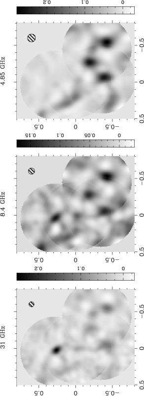
Figure 2: 31 GHz CBI observations of Vela X (a, left). 8.4 and 4.8 GHz MockCBI-processed images are also presented (b and c, middle and right panels respectively). Map center is (08:35:10,–45:27:59), spatial units are in degrees and surface brightness is measured in Jy beam^-1. The hatched ellipse drawn in the top right of each pannel represents each map’s resolution (6.4^′, 5^′ and 4^′ respectively).

After deconvolution, we linearly mosaicked the restored images using the Perl Data Language (PDL). Using all 10 CBI channels we obtained a 31 GHz image of Vela X, shown in Figure 2-a. Repeating the same procedure for the first and last 5 CBI channels, we also produced 33.5 GHz and 28.5 GHz mosaics of Vela X.

3.2 Simulation of the CBI (u,v) coverage on the comparison images

We are interested in computing the spectral index between 8.4 and 31 GHz, by comparing the 31-GHz CBI image with the 8.4-GHz Parkes image from Milne (1995). In Vela X, a network of filaments is superimposed over a smooth plateau, to which the CBI is not sensitive as it lacks total power measurements. Thus, comparison between CBI 31 GHz and single dish 8.4 GHz data is not direct. We simulated the 31-GHz CBI observations over the 8.4-GHz single-dish data, using the MockCBI routine (T.J. Pearson). MockCBI simulates visibilities of any given sky image matching the $uv$-coverage of a reference CBI observation. We therefore produced 4 simulated CBI pointings of Vela X over the 8.4-GHz data, using the identical pointing coordinates and $uv$-coverage than of our original 31 GHz CBI observations. We then repeated with the 8.4 GHz CBI simulated observations the same deconvolution and mosaicking routines applied on the 31 GHz pointings. This procedure provides us with comparable 8.4 and 31 GHz images, as shown in Figure 2-b. We caution that the synthetic beam derived from the CBI $uv$-coverage is $4^{\prime}$ FWHM, while the input 8.4 GHz beam is $3^{\prime}$ FWHM, and the MockCBI-processed 8.4 GHz images has a final resolution of $5^{\prime}$. Although the final resolution of the observed and modelled images are comparable, non-random errors are difficult to quantify (e.g. differences in the deconvolution). These need to be considered when comparing flux densities, particularly on the derived spectral indexes.

In order to include another point for the spectral study of Vela X, we obtained from the Skyview Virtual Observatory an image of the Vela X region at 4.8 GHz, acquired with the Parkes Telescope for the PMN Southern survey (Condon el al., 1993). The original image had $5^{\prime}$ resolution. We tested the calibration of the 4.8 GHz image by computing the integrated flux from two reference sources mapped by the same survey and located near Vela X, the point-sources PMN J1508-8003 and PMN J0823-5010, and comparing with the reference fluxes obtained from the ATCA PMN followup calibrator list. We reproduced the MockCBI, MEM reconstruction and mosaicking procedures applied to the 8.4 GHz data. The resulting 4.8 GHz image is shown in Figure 2-c , and has a final resolution of $6.4^{\prime}$. We note that the image from the PMN survey had missing pointings in Vela, but not in that part of Vela X we are studying (the PWN and the brightest filaments).

3.3 Improvement of the 8.4 GHz image

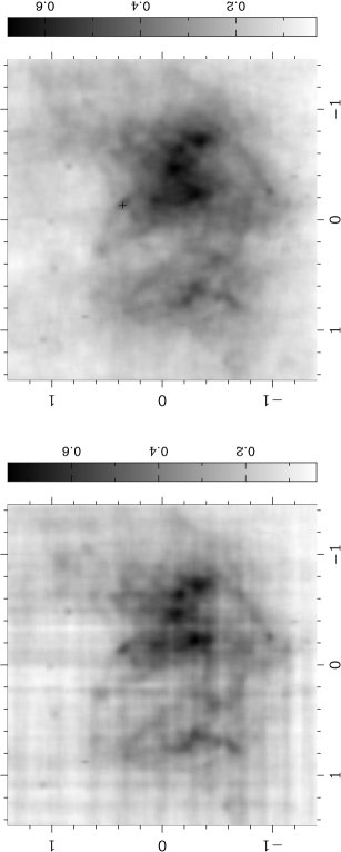
Figure 1: 8.4 GHz archive image before and after destriping. The ($\alpha$, $\delta$) offsets are with respect to (08:36:19.7,–45:23:38.4), units are in degrees. Surface brightness units are in Jy beam^-1, and the Parkes beam FWHM is 3^′. The position of the Vela pulsar is marked with a cross.

Before simulating CBI observations over the 8.4 GHz data, we removed several scanning artifacts that were present in the original 8.4 GHz data. They appeared as many horizontal and vertical lines across the sky image (Figure 1-a). We removed these artifacts by Fourier transforming the sky image and then suppressing contaminating frequencies, which stand out as straight lines crossing the $(u,v)$ origin. We set to zero all visibilities whose moduli differ by more than $3\sigma$ at a given $uv$-radius. Our destriping algorithm follows a standard technique, detailed examples of which can be found in Emerson & Gräve (1988), Davies et al. (1996), and Schlegel et al. (1998). The destriped 8.4 GHz image is shown in Figure 1-b.

4 Results and Discussion

4.1 Vela X at 31 GHz

In Figure 2-a, we present the 31-GHz CBI mosaic of Vela X. We find a strong source around the Vela pulsar position, which we associate with the radio PWN reported and described by Dodson et al. (2003). We measure a FWHM size of $5.9^{\prime}\times 4.1^{\prime}$ in the final MEM-deconvolved image. Alternatively, the model-fit decovolution routine gives an estimated source size of $6.1^{\prime}\times 4.1^{\prime}$. The orientation of the 31 GHz PWN is in agreement with that of the radio lobes seen at higher resolution and at lower radio frequencies (Lewis et al., 2002; Dodson et al., 2003). This object represents the peak of the 31 GHz emission (250 mJy beam^-1), while filamentary structure is observed at low emission levels. Figures 2-b and 2-c show the mosaic images resulting from the simulation of the CBI’s $uv$-coverage on the 8.4-GHz and 4.8-GHz CBI reference images, respectively. Comparison between the three images reveals a marked brightening of the PWN at 31 GHz with respect to both 8.4-GHz and 4.8-GHz images, suggesting that the radio PWN has a flatter spectrum than the rest of Vela X. The spectral analysis of our observations is centered on the comparison between the PWN and the brightest regions of the filaments.

The object we see at the pulsar position is not the Vela pulsar itself. The pulsar is the brightest point source in four 12h observations at 8.4 GHz made with ATCA, at 0.1 arcsec resolution (see Dodson et al. (2003) for more details), with a time-averaged flux density of 32$\pm$12 mJy (Dodson, private communication). This is 1/10 our lowest flux estimate for the PWN and the object we see is not point-like but partially resolved by the CBI 4.1${}^{\prime}\times 4.1^{\prime}$ resolution. Thus we ignored the Vela pulsar contribution in our measures of the PWN fluxes. We also neglected the contamination due to a background radio source near the Vela pulsar at 4.8, 8.4, and 31 GHz since it s 8.4 GHz integrated flux amounts to 7 mJy, or $1/100$ the total PWN flux at 31 GHz (Dodson et al., 2003).

4.2 Fluxes and spectral energy distributions

4.2.1 Flux extraction

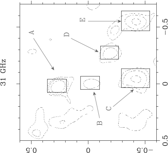
Figure 3: Contour map of Vela X at 31 GHz (30 and 50 percent of peak emission) showing the photometric rectangular apertures (which we also call regions) where integrated flux densities and spectral indexes were computed. They are centered at the peak of each region.

We smoothed the 31 GHz image to match the resolution of the 8.4 GHz MockCBI-processed one, and the resolution of the 28.5 GHz image ($3.9^{\prime}$) to match the resolution of the 33.5 GHz one ($4.8^{\prime}$). We then used a photometric routine for computing the integrated fluxes and spectral indexes of the Vela X brighter components, the PWN and the brighter components of filamentary structure. We measured the integrated flux within the photometric boxes shown in Figure 3. The noise level $\sigma$ was taken as the rms dispersion of pixel intensities in a region of the image that excludes the source. The statistical errors due to noise on the extracted flux densities were estimated by multiplying the noise level $\sigma$ in Jy beam^-1 by $\sqrt{N/N_{\mathrm{beam}}}$, where $N$ is the number of pixels within the aperture (or within the FWHM of the fitted ellipse), and $N_{\mathrm{beam}}$ is taken to represent the number of correlated pixels (those that fall in the FWHM of the beam). This is equivalent to multiplying the noise level in Jy pixel^-1 by $\sqrt{N\,N_{\mathrm{beam}}}$.

The integrated fluxes measured within the photometric boxes (those shown in Figure 3), and their respective statistical errors are presented in Table 1. The 31 GHz measurements are not independent of 33.5 GHz and 28.5 GHz ones, but we quote all three because they are used to compute the 8.4/31 GHz and the 28.5/33.5 GHz spectral indexes separately. The fact that the 31 GHz measurements shown in Table 1 are not equal to the average of the 28.5 GHz and 33.5 GHz fluxes is due to the different resolutions of the three maps. By smoothing the 31 GHz to the resolution of the 28.5 GHz image we obtain 31 GHz integrated fluxes consistent with the 28.5 GHz and 33.5 GHz measurements (In the case of the PWN, the flux at 31 GHz changes from 411 mJy to 421 mJy when matching the 28 GHz resolution). We have also included the 4.8 GHz integrated flux values. In Figure 4 we have plotted the flux density spectrum for region A, corresponding to the Vela radio PWN. Measurements from different epoch and instruments are also shown, but a comparison between them is postponed to Section 4.5. In Figure 5 we have plotted the flux density spectrum for regions C and E, corresponding to the brightest regions of the Vela X filamentary structure at 31 GHz.

At 31 GHz the PWN is approximately elliptical, and its flux can also be obtained by a Gaussian fit. Instead of fitting an elliptical Gaussian to the sky image, we preferred to work with the visibilities on the $uv$-plane, providing us with an alternative (and reconstruction independent) PWN integrated flux computation. Thus, for the compact nebula surrounding the pulsar, we used the model-fitting deconvolution routine implemented in the Difmap data reduction package (Shepherd, 1997). The model-fitting routine essentially matches model visibilities, calculated on a parametrized model image in the sky plane, to the observed ones. We used an elliptical Gaussian component to model the compact radio nebula, whose physical parameters (integrated flux, radial distance, position angle of the center of the component, major axis, axial ratio and position angle of the major axis) are adjusted by the model-fitting routine.

Thus, as an alternative to the photometry flux measurement, we show in Table 2 the integrated flux densities given by the model-fitting deconvolution routine. At 8.4 GHz the integrated flux provided by model-fitting does not represent a good estimate for the PWN, because at 8.4 GHz the modeled ellipse is much larger ($13.1^{\prime}\times 4.5^{\prime}$) than at 31-GHz. This is not related to the frequency-size relationship observed in sources with power-law spatial emission profiles (Reid et al., 1995, for instance), derived from varying beam sizes with frequency, because in our case the 8.4 GHz and 31 GHz beams are very similar (and would be identical if the 8.4 GHz data had a resolution much finer than its 3 arcmin). We doubt the factor of $\sim 2.5$ increase in major axis from 31 GHz to 8.4 GHz is a real feature of the PWN. Rather, it is probably just that the extended emission present at 8.4 GHz contaminates the model-fitting routine. We thus constrained the morphological parameters of the 8.4 GHz model-fitted ellipse in order to match those of the 31-GHz one, leaving just the position and total flux variable. The latter gives a 8.4 GHz flux density value consistent with the one obtained with the photometric routine in a box that approximately isolates the PWN itself: $332\pm 30$ mJy beam^-1 for the size-constrained ellipse compared to $371\pm 20$ mJy beam^-1, the flux density value obtained with the photometric routine. We note that the centroid of the 8.4 GHz constrained ellipse is slightly shifted NE from the 31 GHz one (towards the North-East part of the PWN). This could be related to the steep spectral index measured by Bietenholz, Frail & Hankins (1991) for the North-Eastern lobe, and could explain the large extension of the 8.4 GHz model-fitted ellipse. The discussion on possible morphological changes between 8.4 GHz and 31 GHz is postponed to Section 4.4. At 4.8 GHz the model-fitting routine does not converge.

4.2.2 Spectral indexes

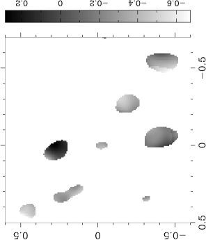
Figure 6: Vela X 8.4/31 GHz spectral index distribution ($5^{\prime}$ beam size). When computing the spectral index image we used a cutoff level of 71 mJy and 51 mJy for the 8.4 and 31 GHz images, respectively. Axis units are in degrees and the center position is as for Fig. 2.

Using the flux values presented in the previous sub-section, we proceeded to compute the Vela X PWN and filaments spectral indexes. We estimated the effects of varying the size of the photometric boxes on the derived spectral indexes, keeping their centers fixed. The systematic uncertainty derived from the box definition dominates over the statistical errors (those coming from flux calculation), and are the ones shown in Table 3, where we present spectral indexes for different regions on the studied frequency bands. Our results reveal that the PWN $\alpha_{8.4}^{31}$ spectral index is positive, with a value of $\alpha_{8.4}^{31}=0.10\pm 0.06$, while the regions of the filamentary structure have an almost uniform negative spectral index, with an average of $\alpha_{8.4}^{31}=-0.28\pm 0.09$ (in which the uncertainty comes from the systematic error linked to the box definition, and from variations between different regions). These results are in agreement with the 8.4/31 GHz spectral index map shown in Figure 6.

The $\alpha_{4.8}^{31}$ and the $\alpha_{28.5}^{33.5}$ spectral indexes were computed after smoothing the higher frequency images to the resolution of the lower frequency ones. The derived spectral indexes are shown in Table 3. The results obtained show similar features to those arising from the 8.4/31 GHz comparison: While the SED of the filaments follows a negative power-law, the PWN’s SED is flat (or even positive). The $\alpha_{8.4}^{31}$ spectral index derived from the model-fitting routine and from the photometric boxes are both positive, but differ at $\sim 2\sigma$. We used the constrained ellipse for the calculation of the 8.4 GHz flux with the model-fitting routine, as we believe it gives better account of the PWN parameters than the unconstrained ellipse. It can be concluded $\alpha_{8.4}^{31}>0.10\pm 0.06$ for the PWN.

The $\alpha_{28.5}^{33.5}$ spectral index is also sensitive to the flux extraction method. But at 26-36 GHz the PWN is very well fit by an elliptical Gaussian, whereas the MEM-restored image is affected by significant negative residuals from the synthetic beam side-lobes. Thus we prefer the $\alpha_{28.5}^{33.5}$ as calculated with the model-fitting routine. However, we chose to fit the 28.5 and 33.5 GHz PWN visibilities with ellipses of constrained size (having the size of the best-fit ellipse for all 10 CBI channels) - unconstraining the ellipses results in a steeper index of $\alpha_{28.5}^{33.5}=-0.45\pm 0.16$. We conclude that $\alpha_{28.5}^{33.5}<-0.25\pm 0.16$.

In summary, $\alpha_{8.4}^{31}$ and $\alpha_{28.5}^{33.5}$ differ at 2$\sigma$, so we suspect a possible spectral break somewhere within 8.4-31 GHz in the SED of the PWN. However, a caveat must be made in the sense that our flux estimations do not take into account non-random errors due to instrumental effects or introduced by differences in the deconvolution. Biases in the total flux densities in MEM deconvolved maps are well known (Cornwell, Braun & Briggs, 1999), as Cornwell-Evans MEM needs the total flux parameter in their approximate MEM optimization. Substantial additional flux has been reported both in simulations and in real observations. These effects may affect our spectral index estimations. In consequence, we caution that the possible spectral break somewhere within 8.4-31 GHz should be considered just as a marginal detection, since it could easily be an instrumental effect. However, our main result still holds: the PWN has a flatter spectral index than the rest of Vela X, as meets the eye in Fig. 2.

4.3 Nature of the Vela X PWN and filamentary structure

The relatively flat SED of the PWN contrasts with the steeper spectrum of the filamentary structure, as clearly seen in Figures 4 and 5. These differences suggest that the PWN is differently, or more recently, energized by the pulsar. Flat spectrum cores are characteristic of pulsar-powered nebulae (Reich, 2002) and are predicted by theoretical models of pulsar winds (Reynolds, 2003). It is possible that the Vela PWN has a flat SED between 8.4 and 31 GHz, and was barely seen at lower radio frequencies since it was hidden by the steep spectrum emission of the radio filaments and diffuse emission. However, it is also possible that the flat PWN SED detected arises from recent particle injection. In Section 4.5 We investigate on the variability hypothesis.

Most authors have agreed on the plerionic nature of Vela X (Dwarakanath, 1991; Alvarez et al., 2001; Bock et al., 1998), but the relationship between the pulsar and the rest of Vela X is still unclear. Our results should provide key pieces in the puzzle of this relationship:

• The spectral indexes we obtain for the filamentary structure are in good agreement with the ones published by Alvarez et al. (2001) for the whole of Vela X. Milne (1995) found no evidence for steepening of the spectrum with increasing distance from pulsar, as would be expected in pulsar-powered remnants. However, our results show that the region surrounding the pulsar does have a flatter SED than the radio filaments.

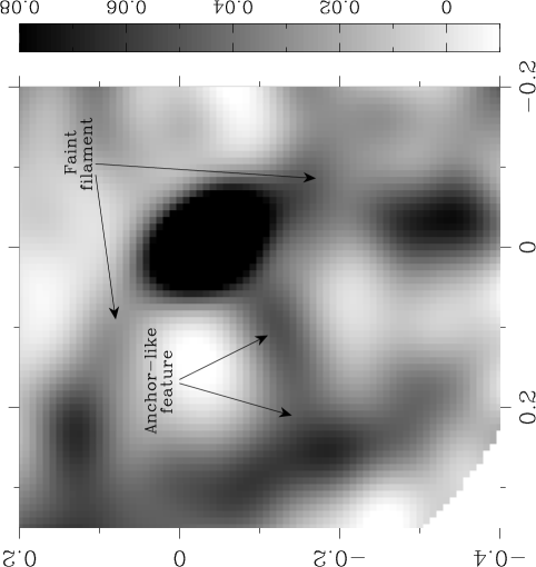
Figure 7: PWN surroundings at 31 GHz. The faint filament extending SW from the PWN and the anchor-like feature are clearly seen. Axis units are in degrees and map center is (08:35:20,–45:10:20).

• In our 31 GHz observations (Figure 2-a), running southwards from the PWN we see the one-sided southern ‘jet’ starting SW from the PWN and then turning South from the PWN, crossing two regions of enhanced emission (regions B and C in Fig. 3). From Figure 7, in which we have zoomed the PWN surroundings, it is apparent that the PWN is linked to the southern ‘jet’ by a faint filament that seems to be an extension of the PWN’s SW lobe. This filament also stands out as a high spatial-frequency structure at 8.4 GHz, as can be seen in the MockCBI-simulated image in Figure 2-b. The possibility of a chance projection of filamentary structure over the PWN is unlikely, because the tangent of the filament at the PWN’s position is parallel to the PWN’s major axis. To further back the above points suggesting pulsar-powered filaments, we note another filament is seen running SE from the PWN, and ending in an ‘anchor-like’ feature, which is located in the direction of proper motion and spin axis of the pulsar. These features are present the MOST mosaic of the Vela SNR by Bock et al. (1998) , although they are more evident in our 31 GHz CBI images. Objects such as G11.2-0.3, G18.95-1.1 and G21.5-0.9, cataloged as plerions and combined-type SNRs, exhibit similar characteristics as the ones described above for Vela X: They exhibit filaments running outwards from a central bar-like feature (Reich, 2002). The central feature in these plerions is thought to be responsible for the particle injection process to the filaments.

• The regions we see as filaments are the ones described by Milne as ‘polarized radio filaments’ (Milne (1995), his Figure 2-b), with the magnetic field directed along these filaments, which he notes is ‘A feature previously seen only in the Crab Nebula (Velusamy et al., 1992)’, and also emphasizes their similar degree of polarization. In Milne’s polarized intensity maps, the PWN is seen at similar polarization fractions than the filamentary structure, and almost completely hidden by diffuse emission in total intensity.

Our observations support aspects of the models by Reynolds (1988) and Blondin et al. (2001). Reynolds (1988) proposed an explanation for filamentary structure in Crab-like SNRs, consisting of thermal filamentary structure (caused by Rayleigh-Taylor instabilities operating on thermal gas accelerated by the pulsar’s wind), interacting with pulsar-generated relativistic particles. Variation in the radio spectrum of the filaments is expected from Reynold’s model, an effect we do not see in Vela X along the filaments, but rather between the radio filaments and the PWN surrounding the pulsar. Blondin et al. (2001) have proposed a model for Vela X in which filamentary structure is not directly pulsar-powered, but rather originated from the Rayleigh-Taylor instability during the crushing of the original PWN by a reverse shock wave that can give account of the filamentary structure’s chaotic appearance and off-center pulsar position. However the model by Blondin et al. (2001) does not address the PWN, and does not explain the spectral properties of the PWN presented in this work and its links with the filamentary structure.

4.4 Morphological changes between the 8.4 GHz and 31 GHz images

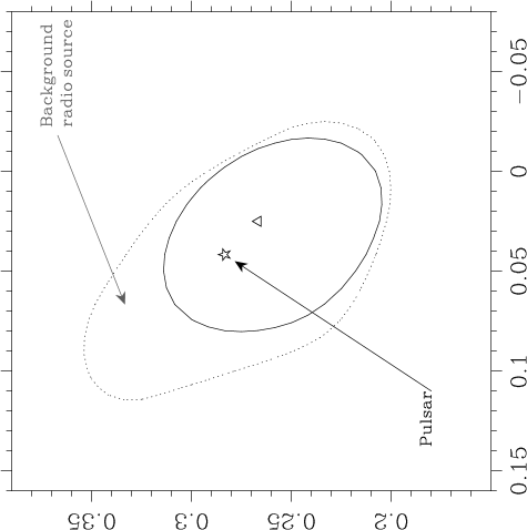
Figure 8: 8.4 GHz (dotted) and 31 GHz (light grey solid) contours at half-maximum, together with the position of the PWN emission maxima (star: 8.4 GHz, triangle: 31 GHz). Axis units are in degrees and center position is as for Fig. 2.

As previously mentioned at the end of Section 4.2.1, the center of the 8.4 GHz and 31 GHz fitted ellipses are offset from each other. This effect is also seen when comparing the position of each image maxima: While at 8.4 GHz the peak of emission approximately coincides with the pulsar’s position, at 31 GHz the maximum emission is shifted in the SW direction. This shift is evident in Figure 8, where we show the position of the PWN emission maxima at 8.4 and 31 GHz, together with the respective contours at half-maximum. We estimated the pointing accuracy of the CBI by analyzing phase calibrator observations, obtaining a $20^{\prime\prime}$ rms pointing accuracy for the Vela observations. The shift between both maxima is thus $85^{\prime\prime}\pm 20^{\prime\prime}$. The shift between the model-fitted ellipse centers (constraining the ellipse size at 8.4 GHz to match that at 31 GHz) is $78^{\prime\prime}\pm 20^{\prime\prime}$.

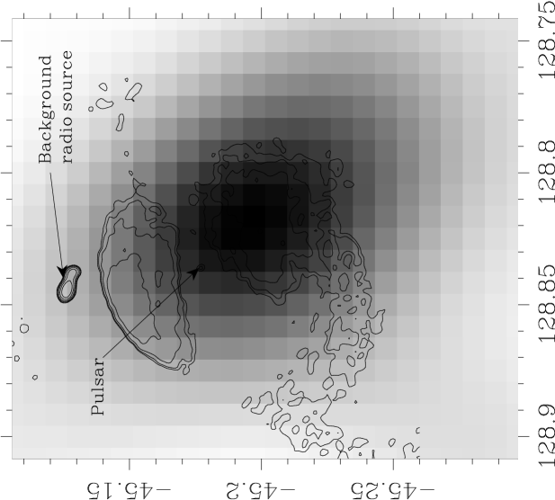
Figure 9: Compact radio source at 5 GHz (contours, ATCA data, Dodson et al. (2003)) and 31 GHz (greyscale). The Vela pulsar and the background radio source are clearly seen.

In Figure 9 we have overlaid a 5 arcsec resolution ATCA map at 5 GHz (Dodson et al., 2003) in contours on the 31 GHz CBI PWN observations in grey scale. In spite of the resolution differences, the shift between the peaks of emission is apparent: it lies in the NE lobe in the ATCA data, while it is closer to the SW lobe in the CBI data. This effect is also seen in the 8/31 GHz spectral index distribution (Figure 6), as a steepening of the PWN spectrum northeastwards. Indeed, this steepening is in agreement with the scaled array VLA observations of Bietenholz, Frail & Hankins (1991), who previously reported the steep spectral index of the NE feature, but did not detect the ‘flat spectrum’ emission from the SW lobe. The spectral index variations detected within the PWN predict morphological changes with increasing frequency.

4.5 Investigation on possible PWN variability

Could the brightening of the region surrounding the Vela pulsar in our 31 GHz data result from variability of the PWN ? This effect have not been reported yet at radio-frequencies, but already evidenced in X-rays by the recent Chandra images of the variable PWN X-ray structure (Pavlov et al., 2003).

PSR B0833$-$45, the Vela pulsar, is characterized by giant glitches, or sudden spin-ups, and is the pulsar where such deviations from steady slow down were first discovered. The latest glitch in the Vela pulsar, which is also the largest spin-up among all glitching pulsars, was recorded in January 2000 (Dodson et al., 2000). As pulsars are the main responsibles for the particle injection in pulsar-powered nebula models, a reasonable question arises : Do giant glitches result in visible changes in the surrounding pulsar-powered nebula ? We suspect variability of the PWN since the integrated flux that we obtain for the PWN at 4.8 and 8.4 GHz from the MockCBI-processed images are well below the values published by Dodson et al. (2003), as may be inferred from Figure 4, where we have plotted ATCA 2001 PWN fluxes, obtained by adding the fluxes from the SW and NE lobes of the PWN published by Dodson et al. (2003). Observation with ATCA in 2001 measure a higher 4.85 GHz flux density than that from the Parkes 1990 image. This increase of the PWN flux between both epochs is probably not merely due to different instrument responses. The difference is opposite to that expected from the ATCA and Parkes responses: because of incomplete sampling in the $uv$ plane the interferometer data is insensitive to small spatial frequencies. However, to perform a reliable flux comparison the single-dish observations should have been modeled onto the interferometer which is being compared (as done for the 8.4/31 GHz data).

The flux density differences may also be influenced by the poor sensitivity of the PMN survey to low spatial-frequency structures. Condon el al. (1993) explain that sources extended more than 30^′ in declination are supressed in the PMN survey. But such spatial frequency corresponds to a $uv-$radius of 115 rad^-1, which is similar the minimum baseline length for the CBI, of 90 rad^-1. Thus a Parkes-CBI comparison based on CBI-simulated images should be accurate at all observed angular scales. The Parkes/CBI comparison of the PWN flux is independent of missing angular frequencies in the PMN data because it is much smaller than the problematic angular scales.

Our CBI observations of the PWN in November 2000 and April 2003, following the Vela pulsar’s January 2000 glitch, showed no evidence of variation of the PWN integrated flux density ($389\pm 8$ Jy and $406\pm 11$ Jy for the 2000 and 2003 observations respectively). It is likely that the differences measured between the Parkes and ATCA observations are due to instrumental/imaging effects overall. Indeed, Bietenholz, Frail & Hankins (1991) did not find any change in the NE feature within the four-months interval of their observations. Our analysis only allows us to conclude that any possible change in the pulsar surroundings must have been produced before our observation epoch, 9 months after the strong January 2000 glitch. This conclusion states that the total flux within a ($5.9^{\prime}\times\,4.1^{\prime}$) elliptical region has varied. Variations in the extension of the region could also be expected, but at the distance of the Vela pulsar (d $287$ pc, as derived from recent VLBI observation by Dodson et al. (2003b)) the $5.9^{\prime}$ FWHM size of the PWN is just about the radius covered by light in 9 months, and is hence unlikely to be detected within the epoch of the CBI observations. It is clear that only high spatial-resolution time-monitoring of the pulsar surrounding can provide reliable conclusions on possible time-dependent changes within the radio PWN.

5 Conclusions

We have detected a strong radio source at 31 GHz around the Vela pulsar, that we identify with the radio pulsar wind nebula (PWN) reported by Dodson et al. (2003). The PWN is surrounded by a low-level network of filaments. We report dramatic changes with frequency in the morphology of Vela X, the pulsar vicinity becoming markedly brighter relative to the rest of Vela X as the frequency increases from 4.8 GHz to 31 GHz. The spectrum of the radio PWN is flat, with an spectral index value of $\alpha_{8.4}^{31}=0.10\pm 0.06$. In contrast, the spectral index of the Vela X filaments is negative, with an average value of $\alpha_{8.4}^{31}=-0.28\pm 0.09$. We investigate whether the flat spectrum PWN obtained in this work reflects the SED of the object or is a consequence of variability (or a combination of both effects), but the lack of consistent comparison data does not allow firm conclusions to be drawn on this subject.

As a step towards understanding the nature of the filamentary structure, we observe that a faint filament crosses the PWN, with a local tangent at the position of the PWN sharing the same position angle as the PWN major axis. This feature might be associated with an extension of the PWN itself. A pulsar-powered nature for the Vela X filaments is also supported by the similarity in morphology and polarization with other plerionic cores.

We detect a shift in the low-resolution centroid of the PWN between 8.4 and 31 GHz, by $80^{\prime\prime}\pm 20^{\prime\prime}$, revealing variations of the spectral index within the PWN. The shift is also evident when comparing the 31-GHz CBI data with high resolution 5-GHz images.

Table 1: Vela X integrated flux densities (mJy).

Frequency (GHz)	Region A†	Region B	Region C	Region D	Region E
33.5	424$\pm$10	262$\pm$20	559 $\pm$15	232 $\pm$15	499 $\pm$30
31	411$\pm$10	261$\pm$30	552 $\pm$15	226 $\pm$15	493 $\pm$30
28.5	418$\pm$16	285$\pm$24	605 $\pm$24	237 $\pm$15	546 $\pm$24
8.4	371$\pm$20	360$\pm$20	662 $\pm$30	375 $\pm$20	716 $\pm$20
4.85	83$\pm$22	248$\pm$20	1040 $\pm$31	963 $\pm$22	1236 $\pm$32

Table 2: PWN flux densities from model-fitting.

Frequency (GHz)	Flux density (mJy)
33.5	529$\pm$40
31	543$\pm$30
28.5	551$\pm$40
8.4	702$\pm$50
8.4 constrained	332$\pm$30

Table 3: Vela X spectral indexes.

Component	$\alpha_{8.4}^{31}$	$\alpha_{4.8}^{31}$	$\alpha_{28.5}^{33.5}$
Region A	0.10$\pm 0.06$	0.75$\pm 0.05$	0.13$\pm 0.11$
model-fit†	0.37$\pm 0.11$		$-$ 0.25$\pm 0.16$
Region B	$-$0.28$\pm 0.12$	$-$ 0.06$\pm 0.11$	$-$ 0.43$\pm 0.15$
Region C	$-$0.16$\pm 0.09$	$-$ 0.41$\pm 0.04$	$-$ 0.35$\pm 0.12$
Region D	$-$0.39$\pm 0.11$	$-$ 0.65$\pm 0.09$	$-$ 0.14$\pm 0.13$
Region E	$-$0.24$\pm 0.09$	$-$ 0.54$\pm 0.03$	$-$ 0.28$\pm 0.21$

Figure 4: Integrated flux density spectrum for region A, corresponding to the radio PWN. The straight line represents the least-squares fit to the 8.4, 28.5 and 33.5 GHz data, given by $\log{F}=(2.482\pm 0.008)+(0.098\pm 0.05)\log\nu$. The CBI and CBI-simulated Parkes error bars represent statistical errors (see Sec. 4.2.1), while ATCA error bars are estimated from variation in the definition of the regions (Dodson et al., 2003). The scatter at low frequencies is discussed in Sec. 4.5.

Figure 5: Integrated flux densities for region C (diamonds, solid line) and region E (filled-circles, dashed line), corresponding to the brightest regions of the filamentary structure. Errors are the statistical estimates due to noise. The straight lines represents the least-squares fits to each region’s integrated flux density, which gave spectral indexes of $\alpha_{\mathrm{C}}=-0.10\pm 0.06$ and $\alpha_{\mathrm{E}}=-0.24\pm 0.04$, respectively. The fit does not include the 4.8 GHz data.

References

- Alvarez et al. (2001) Alvarez, H., Aparici, J., May, J. & Reich, P., 2001, A&A, 372, 636
- Bietenholz, Frail & Hankins (1991) Bietenholz, M.F., Frail, D.A., Hankins, T.H., 1991, ApJ, 376; L41-L44
- Blondin et al. (2001) Blondin, J., Chevalier, R. & Frierson, D., 2001, ApJ, 563, 806
- Bock et al. (2002) Bock, D.C.J., Sault, R.J., Milne, D.K. & Green, A.J., 2002, ASP Conference series, Vol 271, 187
- Bock et al. (1998) Bock, D.C.J., Turtle, A.J. & Green, A.J., 1998, AJ, 116, 1886
- Condon el al. (1993) Condon, J.J., Griffith, M.R. & Wright, A.E., 1993, AJ, 106, 1095
- Cornwell, Braun & Briggs (1999) Cornwell, T.J., Braun, R., Briggs, D.S., 1999, ASP Conf. Ser. 180, 151
- Cornwell & Evans (1985) Cornwell, T.J. & Evans, K.F., 1985, A&A, 143, 77
- Chevalier (2003) Chevalier R.A., 2003, in ”High Energy Studies of Supernova Remnants and Neutron Stars” (COSPAR 2002), Advances in Space Research, in press, astro-ph/0301370
- Davies et al. (1996) Davies, R.D., Watson, R.A. & Gutiérrez, C.M, 1996, MNRAS, 278, 925
- Dodson et al. (2000) Dodson, R.G., McCulloch, P. M. & Costa, M. E., 2000, IAU Circ., 7347, 2, Edited by Green, D. W. E.
- Dodson et al. (2003) Dodson, R.G., Lewis, D., McConnell, D. & Deshpande, A.A., 2003, MNRAS, 343, 116
- Dodson et al. (2003b) Dodson, R.G., Legge, D., Reynolds, J.E., and McCulloch, P., M., 2003, ApJ, 596, 1137
- Dwarakanath (1991) Dwarakanath, K.S., 1991, J.Astrophys.Astr., 12, 199
- Emerson & Gräve (1988) Emerson, D.T. & Gräve, R., 1988, A&A, 190, 353
- Frail & Scharringhausen (1997) Frail, D.A. & Scharringhausen, B.R. , 1997, ApJ, 480, 364
- Frail et al. (1997) Frail, D.A., Bietenholz, M.F., Markwardt, C.B. & Ögelman, H., 1997, ApJ, 475, 224
- Green (2004) Green, D.A., 2004, “A Catalogue of Galactic Supernova Remnants”, Mullard Radio Astronomy Observatory, Cambridge, United Kingdom
- Helfand et al. (2001) Helfand, D., Gotthelf, E. & Halperm, J.P. , 2001, ApJ, 556, 380
- Kennel & Coroniti (1984) Kennel, C.F. & Coroniti, F.V., 1984, ApJ, 283, 710
- Lewis et al. (2002) Lewis, D., Dodson, R., McConnell, D. & Deshpande, A., 2002, in ASP Conf.Ser. Vol 271, Neutron Stars in Supernova Remnants, edited by Slane, P.O & Gaensler, B.M. (San Francisco:ASP), 191
- Markwardt & Ögelman (1995) Markwardt, C.B. & Ögelman, H., 1995, Nature, 375, 40
- Mason et al. (2003) Mason, B. S. , Pearson, T. J., Readhead, A. C. S. , Shepherd, M.C. Sievers, J. L., Udomprasert, P. S., Cartwright, J. K., Farmer, A. J., Padin, S., Myers, S. T., Bond, J. R., Contaldi, C. R., Pen, U.-L., Prunet, S., Pogosyan, D., Carlstrom, J. E., Kovac, J., Leitch, E. M., Pryke, C., Halverson, N. W., Holzapfel, W. L., Altamirano, P., Bronfman, L., Casassus, S., May, J. & Joy, M., 2003, ApJ, 591, 540
- Milne (1995) Milne D.K, 1995, MNRAS, 277, 1435
- Milne & Manchester (1986) Milne, D.K & Manchester R.N., 1986, A&A, 167, 117
- Padin et al. (2002) Padin, S., Shepherd, M.C.j Cartwright, J. K., Keeney, R. G., Mason, B. S., Pearson, T. J., Readhead, A. C. S., Schaal, W. A., Sievers, J., Udomprasert, P. S., Yamasaki, J. K., Holzapfel, W. L., Carlstrom, J. E., Joy, M., Myers, S. T. & Otarola, A. , 2002, PASP, 114, 83
- Pavlov et al. (2001a) Pavlov, G.G., Zavlin, V.E., Sanwal, D., Burwitz, V. & Garmire, G.P., 2001, ApJ, 552, L129
- Pavlov et al. (2001b) Pavlov, G.G., Kargaltsev, O.Y., Sanwal, D. & Garmire, G.P., 2001, ApJ, 554, L189
- Pavlov et al. (2003) Pavlov, G.G., Teter, M.A., Kargaltsev, O.Y. & Sanwal, D., 2003, ApJ, 591, 1157
- Radhakrishnan & Deshpande (2001) Radhakrishnan, V. & Deshpande A. , 2001, A&A, 379, 551
- Rees & Gunn (1974) Rees, M.J. & Gunn, J.E., 1974, MNRAS, 167, 1-12
- Reich et al. (1998) Reich W., Fürst, E. & Kothes, R., 1998, Memorie della Societa Astronomia Italiana, Vol. 69, p.933
- Reich (2002) Reich W., 2002, proceeding of the 270 “WE-Heraeus Seminar on Neutron Stars, Pulsars, and Supernova Remnants.”, ed. Becker, W., Lesch, H., Trümper, J.
- Reid et al. (1995) Reid, M.J., Argon, A.L., Masson, C.R. and Menten, K.M. & Moran, J.M., 1995, ApJ, 443, 238
- Reynolds & Chevalier (1984) Reynolds S.P. & Chevalier R.A., 1984, ApJ, 555, L49
- Reynolds (1988) Reynolds S.P., 1988, ApJ, 327, 853R
- Reynolds (2003) Reynolds S.P., 2003, Proceedings of IAU Colloquium 192 “10 Years of SN1993J”, in press, astro-ph/0308483
- Schlegel et al. (1998) Schlegel D.J., Finkbeiner D.P. & Davis M., 1998, ApJ, 500, 525
- Shepherd (1997) Shepherd M.C., 1997, in Astronomical Data Analysis Software and Systems VI, ed. G Hunt & H.E. Payne, ASP conference series, v125, 77 “Difmap: an interactive program for synthesis imaging”.
- Velusamy et al. (1992) Velusamy, T., Roshi, D. & Venugopal, V.R., 1992, MNRAS, 255, 210
- Weiler & Panagia (1980) Weiler, K.W. & Panagia, N., 1980, A&A, 90, 269