An investigation of the absolute circular polarization in radio pulsars

Abstract

In most pulsars, the circularly polarized component, Stokes $V$, is weak in the average pulse profiles. By forming the average profile of $|V|$ from single pulses we can distinguish between pulsars where $V$ is weak in the individual pulses and those where large $V$ of variable handedness is observed from one pulse to the other. We show how $|V|$ profiles depend on the signal-to-noise ratio of $V$ in the single pulses and demonstrate that it is possible to simulate the observed, broad distributions of $V$ by assuming a model where $|V|$ is distributed around a mean value and the handedness of $V$ is permitted to change randomly. The $|V|$ enhanced profiles of 13 pulsars are shown, 5 observed at 1.41 GHz and 8 observed at 4.85 GHz, to complement the set in Karastergiou et al. (2003b). It is argued that the degree of circular polarization in the single pulses is related to the orthogonal polarization mode phenomenon and not to the classification of the pulse components as cone or core.

1 Introduction

Despite much progress in understanding the polarimetric properties of pulsar radio emission, there remains a number of open and, in some cases, unexplored questions. The basic knowledge that has been obtained over the years is mainly related to three observed phenomena. The first is the observation made by Radhakrishnan & Cooke (1969), that the average polarization position angle (PA) swings across the pulse profile in a way that can be explained by the geometrical rotating vector model, in which the position angle is tied to the direction of the magnetic field lines. As the emission beam of the pulsar sweeps past the line of sight of the observer, an observed swinging PA is a natural consequence. This model has been used to derive the key geometrical angles for a large number of pulsars, such as the inclination angle of the magnetic to the rotational axis and the impact parameter, which determines how close the magnetic axis passes to the line of sight.

The second phenomenon is related to orthogonal transitions observed in the PA of single pulses and integrated pulse profiles. The observation of Manchester, Taylor & Huguenin (1975) that the PA at a particular pulse phase was often observed to be orthogonal to its common value, was taken one step further by Backer, Rankin & Campbell (1976) and Cordes, Rankin & Backer (1978), who identified these PA variations as the manifestation of orthogonal polarization modes (OPM) of emission, anti-parallel to each other on the Poincaré sphere. The link between the PA jumps and the handedness of circular polarization ($V$), noticed by Cordes et al. (1978), was essential to this achievement. The early single-pulse observations permitted the study of the PA at particular pulse longitudes and showed that OPM jumps in single pulses are accompanied by reduced linear polarization $L$, an indication that the observed radiation is in fact the incoherent sum of the emitted OPMs. Stinebring et al. (1984) developed a model in which the polarization properties can be attributed to statistical fluctuations in the OPMs. This model was developed further by McKinnon & Stinebring (1998, 2000) and has been recently extended to account for deviations from mode orthogonality (McKinnon 2003a). Meanwhile, Karastergiou et al. (2001, 2002) showed that the OPM phenomenon was broadband in single pulses, simultaneously observed at different frequencies. Recently, Karastergiou et al. (2003) showed that the association between the handedness of $V$ and the PA becomes weaker towards higher frequencies, indicating that the observed circular polarization cannot straightforwardly be accounted for by existing OPM models.

The third and mostly unexplained observational fact is the high degree of circular polarization in pulsar emission itself. In single pulses, the fractional circular polarization is often quite high, despite the fact that, on average, it usually does not exceed $10\%$ (Han et al. 1998). Radhakrishnan & Rankin (1990) noticed that the average circular polarization observed in central or core components was generally greater than that in the outer or cone components. Another feature of core components is that the integrated $V$ profile is often seen to swing between one and the other handedness. There was a claim that the direction of this change was related to the direction of the swing of the PA (also by Radhakrishnan & Rankin 1990), however, this claim was contested by Han et al. (1998) and Gould (1990).

In this paper, we document the statistics of $|V|$ and provide guidelines for the interpretation of $|V|$ profiles. This is done by examining the dependence of the $|V|$ profile on the distribution of $V$ in the single pulses. Then we proceed to show a number of $|V|$ enhanced integrated profiles from recent polarization observations and finally we discuss the associations of $V$ with OPMs and especially whether there are differences between core and cone emission.

2 Single-Pulse Statistics

The phase-resolved intensity (Stokes $I$) distribution of a number of pulsars has been studied by Cairns et al (2001, 2004). They showed that the statistics are characterised by a log-normal distribution, i.e. that a histogram of the logarithm of the flux densities is normally distributed. Typically, the standard deviation of the distribution is less than 0.3 in the log (see e.g. Johnston et al. 2001, Cairns et al. 2004, Johnston 2004) consistent with the observational evidence that very few pulsars have single pulses with energy more than 10 times the mean energy.

In a study of the Vela pulsar, Kramer, Johnston & van Straten (2002) showed that the distribution of $V$ was strongly correlated with the total intensity distribution. The correlation was not perfect; the distribution of $V/I$ is a Gaussian with the standard deviation determined from both instrumental noise and seemingly intrinsic random fluctuations in $V$. These fluctuations were sometimes large enough that the handedness of the circular polarization changed even though the same orthogonal mode dominated the total intensity. However, the result for Vela is consistent with the earlier, low frequency measurements by Cordes et al. (1978). They showed that the sign of the circular polarization is highly correlated with the mode of the dominant emission; a change of the dominant mode caused a change in sign of circular polarization.

These observations fit in well with the preferred model of orthogonal modes as outlined by McKinnon & Stinebring (1998). In the model, the orthogonal modes occur simultaneously and are 100% polarized. Each mode is associated with a particular handedness of circular polarization. The distribution of $I$ is the result of the sum of the two orthogonal modes and the distribution of $V$ results from the difference of the two modes, as does the distribution of $L$. If the fluctuations of the two modes are perfectly covariant in time, then the difference between them will be constant. This means that the observed degree of $L$ and $V$ will remain constant and no PA jumps will occur. On the other hand, if the covariance between the mode intensities were low, this would result in a variety of observed polarization states. The difference in the OPM intensities would then give rise to broad distributions in $L$ and $V$. Furthermore, non-covariant fluctuations in the OPM intensities can result in switching of the dominant OPM, which is observed as a $90^{o}$ jump in the PA. Therefore, the polarization properties observed in pulsars according to the superposed OPM model, strongly depend on both the mean intensities of the two OPMs and on their covariance.

Recently, however, Karastergiou et al. (2003a), performed high frequency observations of PSR B1133+16. Surprisingly, they discovered that very large values of circular polarization with either sign were present in the data, and that the sign of the circular polarization was not well correlated with the dominant orthogonal mode. Furthermore, in observations of PSR B0329+54, Karastergiou et al. (2001) showed that the outer components of the profile had significant values of circular polarization in single pulses but the distribution was such that the resultant integrated profile had virtually no circular polarization present.

We note that all these studies have been done for bright pulsars with high signal to noise ratios in individual pulses. However, in the majority of pulsars the signal to noise is generally low, especially for circular polarization. This issue was tackled by Karastergiou et al. (2003b, hereafter KJMLE) who used single pulses to construct a profile of the absolute value of circular polarization, $|V|$. They found that the single-pulse behaviour of $V$ is affected, as expected, by OPM jumps, that there are particular pulse phases with significant total power emission that have constant, near zero, circular polarization and that the changes in frequency of $|V|$ profiles are much less significant than the changes in $V$ profiles, indicating that $|V|$ is an important quantity in pulsar emission.

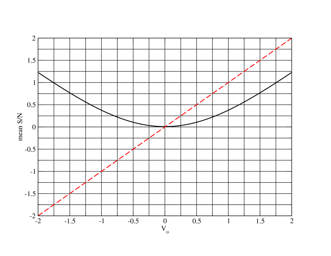
Figure 1: The average S/N in $V$ (dashed) and $|V|$ (solid) is shown against a constant $V_{o}$ in the single pulses, as given by Eq. 1, with $\sigma_{n}=1$. The final S/N obtained by integrating $N$ pulses is $\sqrt{N}$ times the y-axis value.

3 The statistics of $|V|$

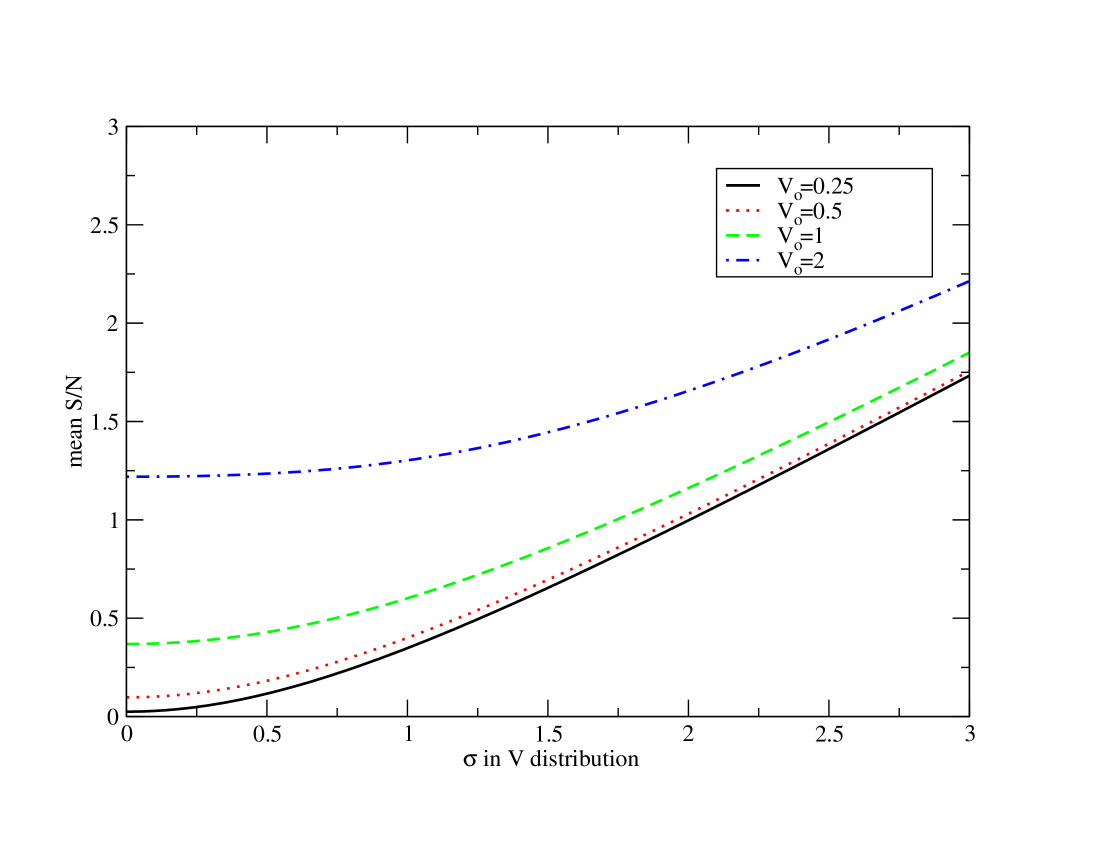
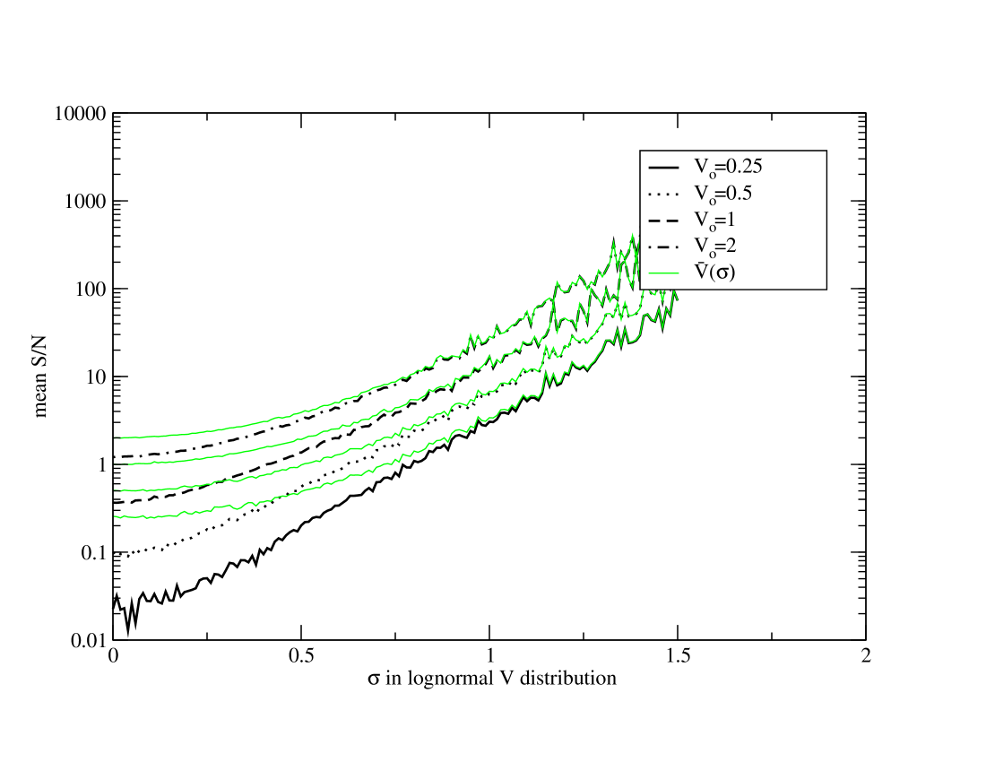
Figure 2: Left panel: The mean S/N in $|V|$, computed from the analytic expression in equation 2, is shown against the $\sigma$ in a Gaussian distribution of $V$, for four values of $V_{o}$. Right panel: The mean S/N in $|V|$ computed from simulations of a log-normal distribution in $V$ for four values of $V_{o}$. Also shown is the mean S/N in $V$. In both panels $\sigma_{n}=1$

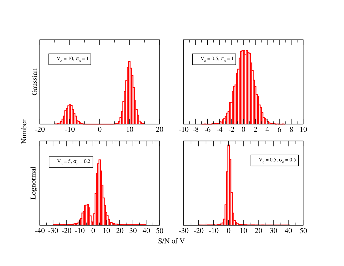
Figure 3: Four simulated distributions of $V$ in single pulses. Each simulation is constructed from an intrinsic $V$ distribution which is bi-modal convolved with Gaussian (receiver) noise. The intrinsic distributions consist of two modes of opposite mean and equal $\sigma$ as denoted; the top panels arise from a Gaussian distribution and the bottom panels from a log-normal distribution. In all cases there are three times as many pulses with positive sign as negative.

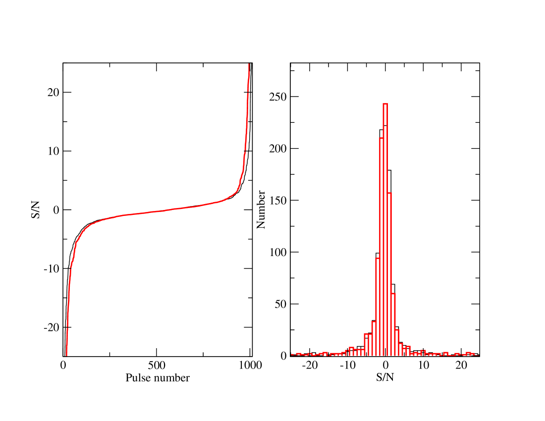
Figure 4: The cumulative (left) and normal (right) histogram of the real (thin black line) and simulated (thick gray line) circular polarization data from pulsar B1133+16.

In observations of single pulses, four Stokes parameters ($I$, $Q$, $U$, $V$) are recorded per phase bin of the pulse period. The off-pulse data have a distribution which is Gaussian with a standard deviation, $\sigma_{n}$, determined by the system noise and are manipulated to ensure a mean of zero. For any symmetrical distribution of $V$ with mean $V_{o}$, the integrated signal after $N$ pulses will be $N\times V_{o}$, the rms of the off-pulse noise will be $\sqrt{N}\times\sigma_{n}$ and hence the resultant signal to noise ratio (S/N) will be $\sqrt{N}\times V_{o}/\sigma_{n}$.

To form the integrated profile of $|V|$ we sum the magnitude of $V$ in the appropriate phase bin for each single pulse. Considering the case where a given phase bin has a Gaussian distribution in $V$ with mean $V_{o}$ and standard deviation $\sigma_{o}$, one can show that $|V|$ will have a mean $\overline{|V|}$ given by

$$\overline{|V|}=\sqrt{\frac{2}{\pi}}\,\sigma e^{\left(\frac{-V_{o}}{\sqrt{2}\sigma}\right)^{2}}+\frac{V_{o}}{\sqrt{\pi}}\int_{\frac{-V_{o}}{\sqrt{2}\sigma}}^{\frac{V_{o}}{\sqrt{2}\sigma}}e^{\left(\frac{-(V-V_{o})}{\sqrt{2}\sigma}\right)^{2}}dV,$$ (1)

where $\sigma=\sqrt{\sigma_{o}^{2}+\sigma_{n}^{2}}$. This can be re-written as

$$\overline{|V|}=\sqrt{\frac{2}{\pi}}\,\sigma e^{\left(\frac{-V_{o}}{\sqrt{2}\sigma}\right)^{2}}+V_{o}{\rm erf}\left(\frac{V_{o}}{\sqrt{2}\sigma}\right),$$ (2)

with $\rm erf$ being the error function, defined as:

$${\rm erf}(x)=\frac{2}{\sqrt{\pi}}\int_{0}^{x}e^{-t^{2}}dt.$$ (3)

Consider equation 1 for the off-pulse emission which has $V_{o}=0$ and $\sigma=\sigma_{n}$. In this case the mean off-pulse signal which we denote $\overline{|V|}_{n}$ is simply

$$\overline{|V|}_{n}=\sqrt{\frac{2}{\pi}}\,\sigma_{n}.$$ (4)

In order that the off-pulse region of the profile of $|V|$ have a zero mean therefore, we must subtract $\overline{|V|}_{n}$ from each phase bin of each profile. The S/N in each bin of the $|V|$ profile is then

$${\rm S/N}=\left(\frac{\overline{|V|}}{\sigma_{n}}-\sqrt{\frac{2}{\pi}}\right)\sqrt{N}$$ (5)

When we refer to $|V|$ hereafter, we are actually referring to $\overline{|V|}$ from the above equations and, in particular, when we refer to the S/N of $|V|$, it is given by Equation 5. Figure 1 shows the S/N in $|V|$ compared to $V$ as a function of $V_{o}$ in the single pulses, assuming $\sigma_{n}=1$ and $\sigma_{o}=0$ (i.e. that the intrinsic $V$ distribution is a delta function). It is apparent that for values of $V_{o}$ greater than $\sim 1$, the S/N in $|V|$ builds up linearly but for values below this the S/N in $|V|$ builds up at a slower rate. However, because we are forced to subtract the baseline, the signal to noise in $|V|$ is always less than in $V$ (when $\sigma_{o}=0$). Figure 2 shows the S/N in $|V|$ as a function of $\sigma_{o}$ for four values of $V_{o}$. The S/N in $|V|$ increases with $\sigma_{o}$,whereas, because the distribution is symmetrical, the S/N in $V$ is independent of $\sigma_{o}$. There are two main points to be gleaned from these figures. The first is that the S/N in $|V|$ cannot be less than the case where the distribution of $V$ is a delta function (i.e. $\sigma_{o}=0$). We can therefore construct a ‘minimum profile’ of $|V|$ from the mean $V$ in each phase bin. The second point is that, under the assumption of a Gaussian distribution of $V$, one can determine $\sigma_{o}$ by comparing the S/N in $|V|$ and $V$.

As discussed in the previous section, the distribution of $V$ may be log-normal rather than Gaussian. In this case, the convolution of the log-normal distribution with the Gaussian noise is not trivial analytically. We have therefore treated the problem numerically and present the results in the right hand panel of Figure 2. The median S/N is the same as the mean S/N in the left hand panel of the figure, and the sigma is now in the log. It can be seen that the mean $|V|$ rapidly increases as a function of $\sigma_{o}$, much more rapidly than in the Gaussian case. However, the mean of $V$ also increases rapidly with $\sigma$. As a result, for typical values of $\sigma$ ($\sigma<1$), it remains that $|V|<V$.

So far, we have only considered unimodal distributions of $V$. In Karastergiou et al. (2003a) and KJLME it was shown that large values of $V$ of either handedness occur irrespective of the dominant OPM, which suggests that the handedness of $V$ may be set randomly. We therefore make the simplistic assumption that $V$ is always generated with a positive sign and introduce the parameter $F$ to denote the fraction of data in which the sign of $V$ changes (i.e. $0.0<F<1.$). It is for distributions with $F\approx 0.5$ that $|V|$ becomes a very powerful tool as the S/N in $|V|$ is independent of $F$ whereas the S/N in $V$ is reduced by a factor $1-2F$.

Figure 3 shows examples of simulated data chosen from bi-modal Gaussian and log-normal distributions, where $F=0.25$. In cases where the S/N is high (left-hand side panels), the two components are clearly separated. However, in cases of low S/N (right-hand side panels), the convolution with the noise merges the distributions. This means that in the Gaussian, low S/N case (top right), the deconvolution to determine the underlying distributions does not lead to a unique solution. In the log-normal, low S/N case (bottom right) however, the parameters of the parent distribution are much better constrained: it must be bimodal ($F\neq 1$ and $F\neq 0$) and $V_{o}$ and $\sigma$ are constrained by the characteristics of the positive and negative tails of the distribution. We note that in real pulsar observations, distributions like the high S/N cases on the left hand side have not been observed. However, this may be purely due to the low S/N in single-pulse observations. An increase in sensitivity in the future will reveal whether such “separated” distributions are real.

What remains to be tested is whether the three parameters we introduced can describe observational data. Each set of $V_{o}$, $\sigma$ and $F$ values are used to simulate a particular distribution. We then apply a Kolmogorov-Smirnoff (K-S) test (Press et al. 1992) to compare the real and simulated distributions of $V$. The K-S test returns the probability $P$ that the two compared datasets do not originate from the same distribution. A concrete example involves PSR B1133+16 data at 4.85 GHz. In the relevant profile of Figure 1 of KJMLE, $|V|$ has a maximum in the leading component and we examine this particular phase bin. The S/N in the integrated profile (over a total of 1013 pulses) of that bin is $V=-3.8$ and $|V|=82.1$. We find that the intrinsic $V$ distribution which best reproduces the data is a log-normal distribution with $|V_{o}|=0.43,\sigma=0.95$ and $F=0.64$. Figure 4 shows how good the simulation is in fitting the observed data. The thick line in the two histograms corresponds to the real data and the thin line to the simulation. The claim that the underlying $V$ distribution is bimodal is somewhat contrary to the visual impression given by Figure 4. However, in the context of our model where the distribution of $|V|$ is either Gaussian or log-normal and a sign change occurs in a fraction of the pulses, this particular distribution can only be adequately described by a bimodal solution. This is no surprise, given that the observed $V$ distribution closely resembles the bottom right simulated distribution of Figure 3. The fact that this solution describes the observed data very well, shows that our model works. Also, the K-S test is more sensitive around the median value which is the reason our method overestimates $\sigma$, causing the disagreement seen in the tails of the cumulative distribution.

From the above description we can see how the combination of $|V|$ and $V$ can reveal details of the underlying distributions in each phase bin, without needing to perform the tedious task of constructing and analysing the $V$ distribution itself. In summary, there are 3 possibilities which can occur. First, that $|V|$ is significantly larger than the magnitude of $V$. This can occur either because the parameter $F$ is close to 0.5 and/or because the width of the underlying distribution is large. The second possibility is that $|V|$ and $V$ are about the same magnitude. In this case, $F$ must be near 0 or 1 and/or the width of the underlying distribution must be small relative to the mean. Finally, $|V|$ can be less than the magnitude of $V$. This can occur in low signal-to-noise regimes (cf Figure 1) provided that the width of the distribution is not large.

4 Enhanced pulsar profiles

Having shown that our simple model describes the data well, we show 13 profiles of pulsars including $|V|$ and extract conclusions about the behaviour of circular polarization in single pulses.

The data consist of observations of single pulses from 13 northern pulsars, 5 at 1.41 GHz and 8 at 4.85 GHz, to complement the sample of KJMLE. We used the Effelsberg 100-m telescope in observations that took place between July and September 2002. The data were carefully calibrated according to a revised scheme based on von Hoensbroech & Xilouris (1997). Both the 4.85 and the 1.41 GHz system had a system equivalent flux density of $\approx 20$ Jy. We used a bandwidth of 500 MHz at 4.85 GHz and a choice between 10, 20 and 40 MHz at 1.41 GHz. The pulsars in our sample were chosen to have a reasonably small dispersion measure (DM) due to the limitations of the backend used and the choice of bandwidth at 1.41 GHz was based on each particular DM.

In Figures 5 and 6, we plot the average profile of the total power, of circular polarization $V$ and the profile of $|V|$, which is computed as described in Section 3, by subtracting the noise offset from each single pulse. For clarity, we have not included the linear polarization nor the position angle swing for these pulsars, but we have used all the polarization information contained in the integrated profiles and the single pulses where relevant.

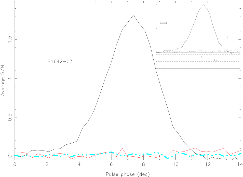
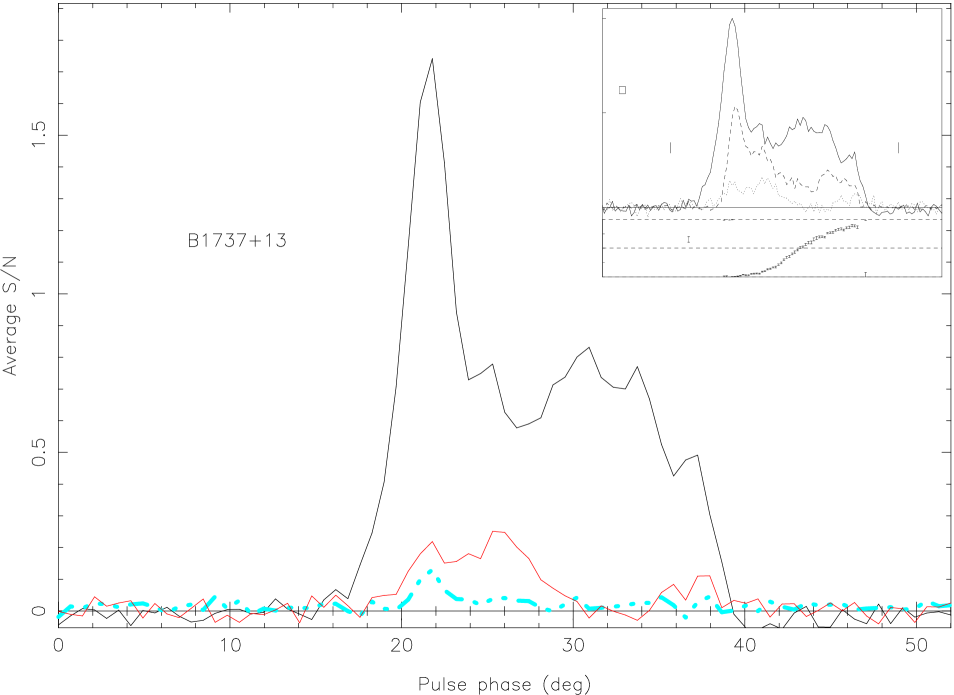
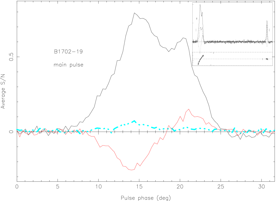
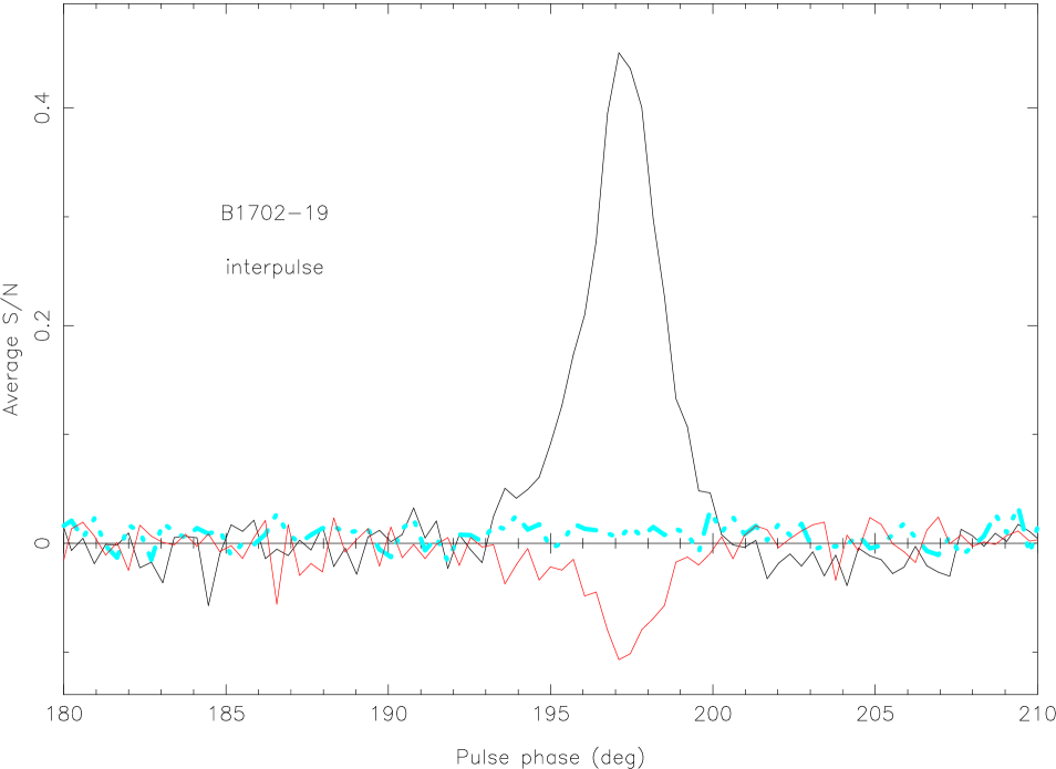
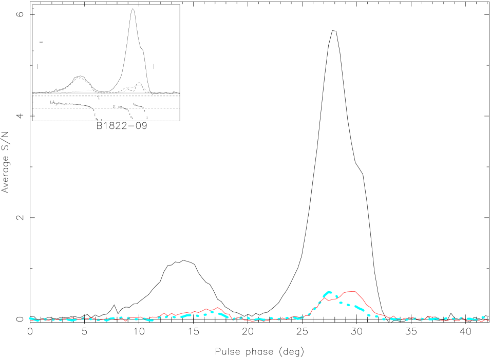
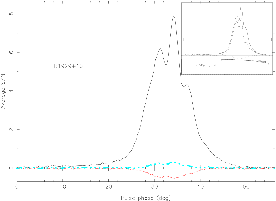
Figure 5: Integrated profiles of 5 pulsars at 1.41 GHz. Both the main pulse and interpulse are shown for PSR B1702$-$19. The average S/N of the total intensity $I$ and the circular polarization $V$ are shown with thin lines, the $|V|$ profile is shown with a thicker, dot-dashed line. The inserts represent the full polarization profiles, including $L$ (dashed line), and the PA ranging from $-90^{o}$ to $90^{o}$.

4.1 Profiles at 1.4 GHz

PSR B1642$-$03: The integrated profile of PSR B1642$-$03 at 1.4 GHz consists of a single component which shows virtually no linear or circular polarization. Lyne & Manchester (1988, hereafter LM) classify this pulsar as a core single. We find that the profile of $|V|$ is just like that of $V$, with $S/N\approx 0$ across the entire component and, furthermore, we do not see any highly linearly polarized single pulses. We conclude that the individual pulses are not highly circularly polarized. The evidence points to the fact that the two competing orthogonal modes are equally strong and highly correlated.

PSR B1702$-$19: The average profile of PSR B1702$-$19 shows a swing of $V$ from negative to positive. The profile of this pulsar is classified as cone-dominated in LM. However, the steep position angle swing of the linear polarization and the presence of a phase bin near the centre where both $V$ and $|V|$ are zero make it more likely that this is a core component. At the pulse phase where $V$ changes handedness, $|V|\approx 0$. This is a common feature pointed out by KJMLE, implying that at this particular phase bin the circular polarization is consistently a small fraction of $I$. The S/N of the single pulses is low and we cannot draw many conclusions from the profile of $|V|$. However, it is likely that the swing of $V$ is a feature of the single pulses. The interpulse, shown in the next panel of the same figure, is almost 100% linearly polarized and only weakly circularly polarized. The low S/N in $V$ forces the profile of $|V|$ to be zero, so the conclusion is that there are no pulses where the interpulse is highly circularly polarized.

PSR B1737+13: There are a number of pulsars with profiles that consist of both cone and core components. In PSR B1737+13, the profile also exhibits a very smooth position angle swing and a relatively high degree of linear polarization, although again the circular polarization across the profile is low. More specifically, in the leading component, $V$ has a peak value of 0.22. If the intrinsic $V$ distribution were a delta-function, Figure 1 suggests that $|V|$ should have a very small value ($<<0.1$). In reality, the measured value is $|V|\approx 0.15$, which would be the result of a $V$ delta-function at $V_{o}\approx 0.5$. We therefore can deduce that either a sign-changing effect reduces $V$, or the distribution of $V$ has some intrinsic width that makes the distribution wider and gives rise to some values of opposite handedness. The linear polarization under the peak is $\approx 50\%$ and makes for a good comparison with the next component. In that, $L$ is a significantly higher fraction of $I$, but $|V|$ is very weak compared to $V$, implying a narrow distribution around $V_{o}$. In the centre of the profile of this pulsar also, $V=|V|=0$.

PSR B1822$-$09: The profile of this pulsar consists of the main pulse and an interpulse, which both exhibit a peculiar moding behaviour (Fowler & Wright 1982 ). We focus only on the main pulse, mainly due to the low S/N of the interpulse. LM suggest that both the leading and trailing component of the main pulse are conal. The leading component is highly linearly polarized. As far as the circular polarization is concerned, the leading component of the main pulse is weak in both $V$ and $|V|$ and it is likely that the circular polarization is generally low in the single pulses. In the trailing component of the main pulse, however, $|V|$ is as high as $V$. We also see evidence for a bi-modal position angle distribution. In this component therefore, it appears as if $V$ is often large and of variable sign in order to give rise to a large $|V|$.

PSR B1929+10: The profile of PSR B1929+10 is almost entirely linearly polarized. The swing of position angle across the pulse is rather flat and the profile is classified as conal by LM. Both $V$ and $|V|$ in the integrated profile are low. The results for this pulsar are very similar to that seen in the Vela pulsar (Kramer et al. 2002). A single orthogonal mode dominates throughout, the single pulses are highly linearly polarized and have a largely constant sign of circular polarization.

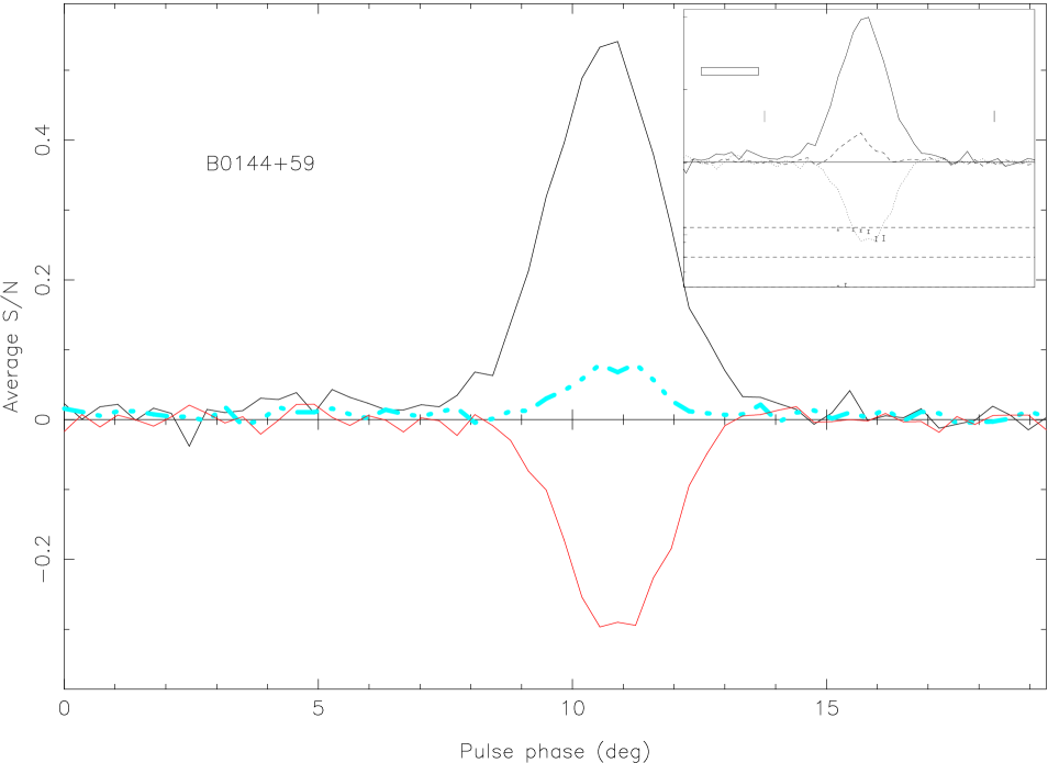
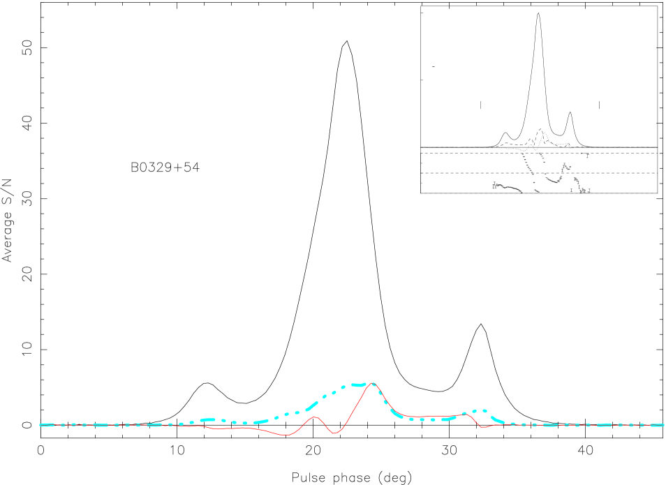
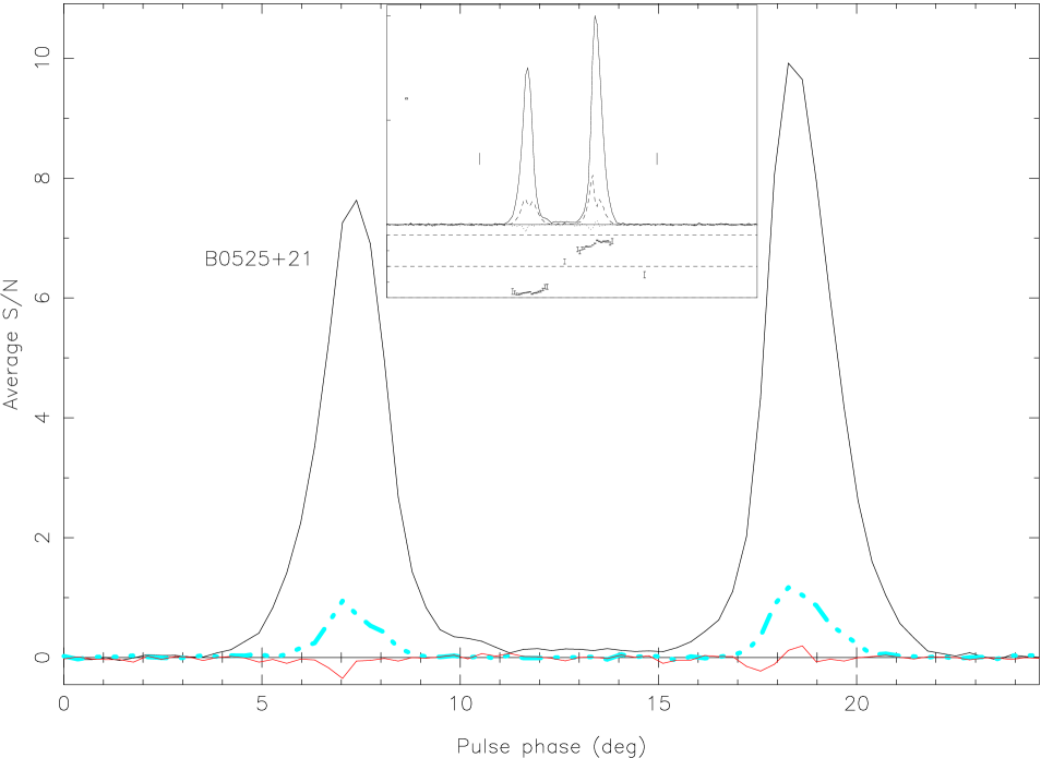
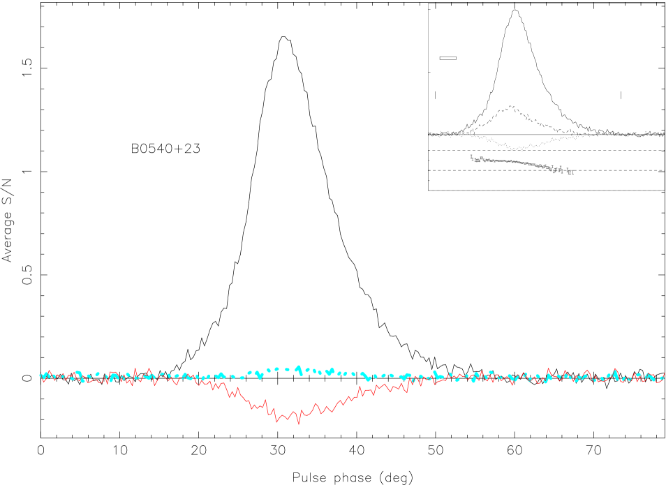
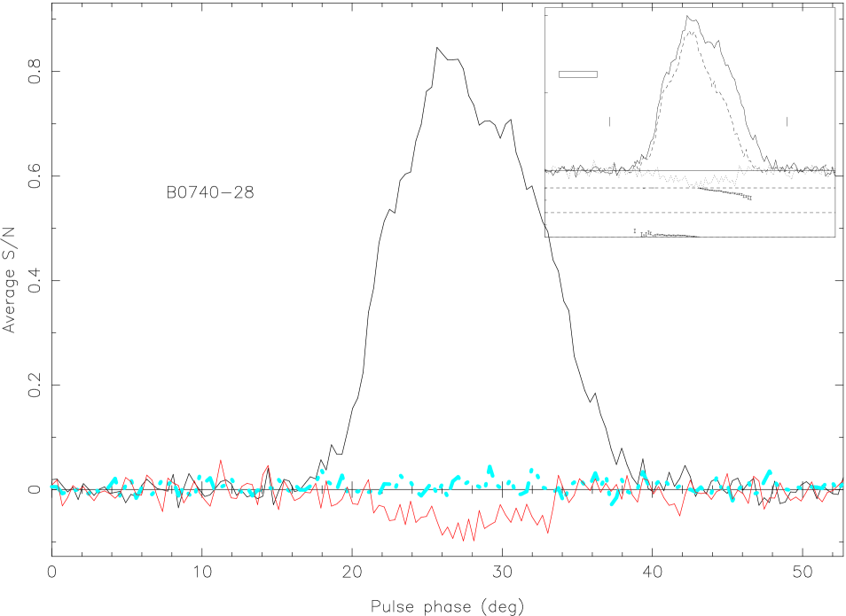
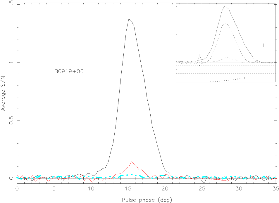
Figure 6: Integrated profiles of 6 pulsars at 4.85 GHz. The lines and the inserts are explained in Figure 5.

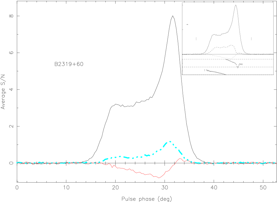
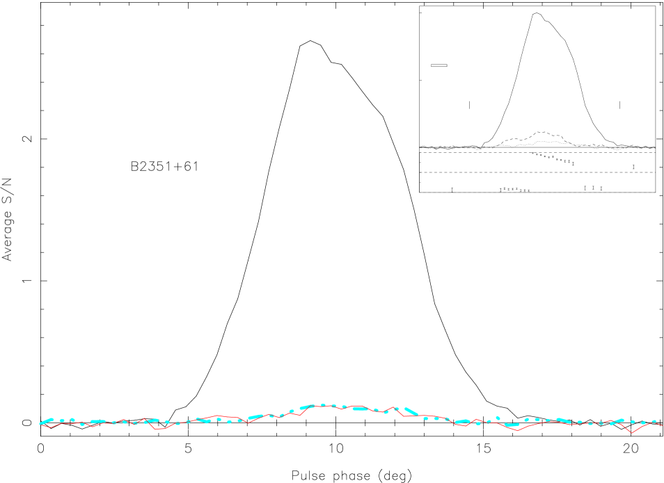
Figure 6: …continued.

4.2 Profiles at 4.85 GHz

PSR B0144+59: PSR B0144+59 has not been classified by LM, but the flat position angle swing of the linear polarization is characteristic of conal emission. The integrated profile has a very high degree of right-hand circular polarization, one of the highest fractional circular polarizations of any pulsar. The $|V|$ profile is that expected from the low S/N and an almost constant value of $V$. It seems unlikely that there are single pulses with strong positive circular polarization.

PSR B0329+54: The polarization profile of PSR B0329+54 at 4.85 GHz is very complex. The linear polarization drops suddenly to local minima at two pulse phases, the handedness of the circular polarization changes a number of times and the position angle shows a number of kinks and jumps (as has been noted before by other authors, e.g. Gil & Lyne 1995). The profile of $|V|$ is much less complicated than the profile of $V$. In fact, it traces the average profile of the total power well, so that the quantity $|V|/I$ remains fairly constant across the pulse. In the leading and trailing components, $|V|>V$ and at the same time, competing OPMs are evident through the reduced linear polarization and OPM jumps in the single pulses. Also, in the leading part of the middle component, $V$ changes handedness on three occasions, OPM jumps and local minima of $L$ are seen and $|V|$ is significantly greater in amplitude than $V$. In fact, at the phase bin just after $22^{o}$ in Figure 6, the average S/N in $|V|$ is $\approx 6$ whereas $V_{o}=0$. The actual distribution resembles the PSR 1133+16 example of the previous section: it is clearly log-normal and bimodal, while the linear polarization has a local minimum. The same thing holds for the phase bin at $32^{o}$.

PSR B0525+21: PSR B0525+21 is a long period pulsar with a distinctive double profile of conal components. The overall polarization in the integrated profile is low, neither component shows significant $V$. However, the profile of $|V|$ has a reasonably large amplitude. This implies that there must be a number of highly circularly polarized single pulses, of either handedness. At the same time, even though no orthogonal jumps are seen in the position angle in the integrated profile, the position angle has a bimodal distribution in the single pulses.

PSR B0540+23: LM classified the profile of PSR B0540+23 as conal based on the flat position angle swing. There are no OPM jumps in the position angle and there is a moderate amount of linear polarization in the profile. Despite the fact that at 4.85 GHz, it shows a moderate amount of circular polarization, the profile of $|V|$ indicates that there generally is a constant sign of $V$ in the single pulses. The results for this pulsar therefore resemble those for Vela and PSR B1929+10.

PSR B0740$-$28: LM classify this pulsar as having conal emission. There is a high degree of polarization and no evidence of OPM jumps in the single pulses. Similar to PSR B0540+23, this pulsar is very weak in both $V$ and $|V|$. Although the S/N is not high in total intensity in this pulsar, it can be compared directly with PSR B1702$-$19 which has a similar S/N but has a significant amount of $|V|$. The profile of $|V|$ suggests that the circular polarization in the single pulses is generally low with few high values of either handedness seen.

PSR B0919+06: PSR B0919+06 is considered to have partial cone emission by LM, has a very similar profile to PSR B1929+10 and similar polarization features to Vela. The profile of $|V|$ suggests that the single pulses are only moderately circularly polarized.

PSR B2319+60: PSR B2319+60 is a strong pulsar with both core and cone emission, according to LM. At first glance the profiles of $V$ and $|V|$ at 4.85 GHz look like mirror images of each other. A closer look, however, at the trailing edge of the profile reveals that $|V|$ remains large at the phase where $V$ changes handedness. This change in handedness in $V$ coincides with a kink in the position angle swing, which is not quite an orthogonal jump. At the same phase, the distribution of position angles in the single pulses is bimodal. As with PSR B0525+21, there are many single pulses with significant $V$ of either handedness.

PSR B2351+61: PSR B2351+61 has low linear polarization and also shows an OPM jump in the position angle swing. As with PSR B1133+16, the lack of polarization at high frequencies is indicative of a lack of correlation between the mode strengths. The single pulses show a bimodal distribution of position angles throughout the pulse profile. The profile of $|V|$ is slightly greater than that of $V$. This shows that there are pulses with significant $V$ of either sign in the single pulses. This is similar to PSRs B1133+16 and B0525+21.

PSR name	Classification		Degree of	Bimodal PA	$|V|=V=0$	$|V|>V$
	cone	core	polarization	distributions	in core
B1642$-$03		$\surd$	low		$\surd$
B1702$-$19		$\surd$	medium		$\surd$
B1702$-$19(interpulse)	$\surd$		high
B1737+13	$\surd$		medium
B1737+13		$\surd$	low		$\surd$
B1822$-$09(leading)	$\surd$		high
B1822$-$09(trailing)	$\surd$		low	$\surd$		$\surd$
B1929+10	$\surd$		high
B0144+59	$\surd$		high
B0329+54	$\surd$		low	$\surd$		$\surd$
B0329+54		$\surd$	low	$\surd$		$\surd$
B0525+21	$\surd$		low	$\surd$		$\surd$
B0540+23	$\surd$		medium
B0740$-$28	$\surd$		high
B0919+06	$\surd$		high
B2319+60	$\surd$		medium/low	$\surd$		$\surd$
B2319+60		$\surd$	medium
B2351+61	$\surd$		low	$\surd$		$\surd$

Table 1: A summary of the properties seen in the enhanced average profiles.

5 Discussion and conclusions

The pulsars observed are listed in Table 1, in some instances with individual components occupying a separate entry. In columns 2 and 3 of the table we show the classification of the pulsar/component as core or cone. Column 4 lists the degree of polarization in three broad categories, as high, medium or low. In column 5 we indicate if bimodal PA distributions are present. Columns 6 and 7 denote the relationship between $|V|$ and $V$. If neither column 6 nor 7 apply, it is implied that $V>|V|$.

Table 1 shows a clear correlation between the presence of bimodal PA distributions, low overall polarization and $|V|>V$. This is expected in the superposed model of OPM: the low polarization indicates the modes are almost equally strong and, if their amplitudes are not perfectly covariant, a bimodal distribution of PA will ensue. The integrated $V$ will be low, although individual pulses can show high values of $V$ of either handedness. The fact we observe $|V|>V$ is a strong indicator of wide, bimodal distributions of $V$ in the single pulses. However, the low mean $V$ compared to the noise makes the observed distribution appear unimodal (see Figure 3).

The degree of polarization in pulsars is generally higher at 1.4 GHz than at 4.85 GHz, as was identified by e.g. Manchester (1971), Xilouris et al. (1996), von Hoensbroech, Lesch & Kunzl (1998). This was explained by a superposed OPM model, in which the two modes become equally strong with increasing frequency (Karastergiou et al. 2002), who also showed that the degree of covariance between the OPMs decreases with increasing frequency. Low covariance between the OPMs means that the difference in the intensities of the two modes can have a value which fluctuates significantly in time. It is this difference that determines the observed polarization (linear, circular and PA), therefore, as a result, broader distributions in linear and circular polarization and bimodal PAs are observed. The pulsars in Table 1 support this model: not only does the total degree of polarization decrease with frequency, but also the high $|V|$ profiles (i.e. broad $V$ distributions) indicate a low degree of correlation between the OPMs. However, low covariance is not enough to explain the high frequency results. A test of the requirement of the OPM model, that each OPM is associated to a particular sense of $V$, fails for the pulsars that show bimodal PA distributions. The behaviour seen in these pulsars resembles that of PSR B1133+16, which strongly suggests that the above OPM model needs some adjustment. This can be achieved by a statistical model where the sign of $V$ is set randomly as in the model we have presented here, but the underlying physical reasons remain unclear. A possible explanation could arise by considering the altitude from the pulsar surface at which the polarization characteristics are set. At lower heights one may expect that the regions of positive and negative charge fluctuate on short time scales, generating greater randomness in the polarization properties of the higher frequency emission. As the plasma streams outwards, it becomes more homogeneous, so the lower frequency polarization properties fluctuate less. It is, however, very important to stress that the sign-changing process is only present when bimodal PA distributions are observed, suggesting a common origin of these two phenomena.

In the pulsars of our sample that show no evidence of bimodal PA distributions, $V\geq|V|$. The relationship between $V$ and $|V|$ therefore appears to be related to the type of PA distributions, regardless of the classification of the component. This is highlighted in PSR B0329+54, where both the core and cone components show bimodal PA distributions and $|V|>V$. In our sample, bimodal PA distributions are predominantly observed in cone components. We therefore suggest that the low degree of average circular polarization in cone emission is not intrinsic to the emission mechanism, but rather due to broad, symmetrical distributions of $V$ which are correlated with bimodal PA distributions. Pulsars with the same characteristics were also identified in KJMLE. In particular, PSRs B0950+08, B1133+16 and 2020+28 show $|V|>V$ together with bimodal PA distributions. All three of these pulsars exhibit the aforementioned OPM frequency dependence.

We have identified three pulsars in which $V$ swings from one sign to the other in the average profile and $|V|=0$ at the same phase bin as $V=0$. KJMLE also identified 3 such pulsars (PSRs B1508+55, B1933+16 and B2111+46) and argued that these phases correspond to constant, very low circular polarization. However, such swings in the handedness of $V$ are also often seen in cone components in the single pulses. It would therefore be interesting to identify a pulsar that has a cone component, no OPM jumps and a $V$ profile that shows this signature. We predict that $|V|$ will behave in the same way as it does in the core components, i.e. there will be a phase bin where $V=|V|=0$. This will demonstrate that the $V$ swing is not a distinguishing feature between cone and core emission and it is for other reasons, such as jittering in pulse-phase of cone components, that such swings are usually only seen in the average profiles of core components.

In conclusion, forming the integrated profile of $|V|$ provides information not available from the $V$ profile alone. Our main results are 1) that pulse components with bimodal PA distributions also show wide distributions of $V$, 2) that there is little difference in the circular polarization between core and cone components except that the swing of $V$ seen in core components is generally maintained in the single pulses and 3) that the degree of polarization and the covariance between the modes are less in the pulsars observed at the highest of the two frequencies, as expected by previous studies, while at the same time the handedness of $V$ is less correlated with the dominant OPM.

References

- Backer et al. (1976) Backer D. C., Rankin J. M., Campbell D. B., 1976, Nature, 263, 202
- Cairns et al. (2001) Cairns I. H., Johnston S., Das P., 2001, ApJ, 563, L65
- Cairns et al. (2004) Cairns I. H., Johnston S., Das P., 2004, MNRAS, Submitted
- Cordes et al. (1978) Cordes J. M., Rankin J. M., Backer D. C., 1978, ApJ, 223, 961
- Fowler & Wright (1982) Fowler L. A., Wright G. A. E., 1982, A&A, 109, 279
- Gil & Lyne (1995) Gil J. A., Lyne A. G., 1995, MNRAS, 276, L55
- Han et al. (1998) Han J. L., Manchester R. N., Xu R. X., Qiao G. J., 1998, MNRAS, 300, 373
- Johnston (2004) Johnston S., 2004, MNRAS, 348, 1229
- Johnston et al. (2001) Johnston S., van Straten W., Kramer M., Bailes M., 2001, ApJ, 549, L101
- Karastergiou et al. (2003) Karastergiou A., Johnston S., Kramer M., 2003, A&A, 404, 325
- Karastergiou et al. (2003) Karastergiou A., Johnston S., Mitra D., van Leeuwen A. G. J., Edwards R. T., 2003, MNRAS, 344, L69
- Karastergiou et al. (2002) Karastergiou A., Kramer M., Johnston S., Lyne A., Bhat R., Gupta Y., 2002, A&A, 391, 247
- Karastergiou et al. (2001) Karastergiou A. et al., 2001, A&A, 379, 270
- Kramer et al. (2002) Kramer M., Johnston S., van Straten W., 2002, MNRAS, 334, 523
- Lyne & Manchester (1988) Lyne A. G., Manchester R. N., 1988, MNRAS, 234, 477
- Manchester (1971) Manchester R. N., 1971, ApJS, 23, 283
- Manchester et al. (1975) Manchester R. N., Taylor J. H., Huguenin G. R., 1975, ApJ, 196, 83
- McKinnon (2003) McKinnon M. M., 2003, ApJ, 590, 1026
- McKinnon & Stinebring (1998) McKinnon M., Stinebring D., 1998, ApJ, 502, 883
- McKinnon & Stinebring (2000) McKinnon M. M., Stinebring D. R., 2000, ApJ, 529, 435
- Press et al. (1992) Press W. H., Teukolsky S. A., Vetterling W. T., Flannery B. P., 1992, Numerical Recipes: The Art of Scientific Computing, 2nd edition. Cambridge University Press, Cambridge
- Radhakrishnan & Cooke (1969) Radhakrishnan V., Cooke D. J., 1969, ApL, 3, 225
- Radhakrishnan & Rankin (1990) Radhakrishnan V., Rankin J. M., 1990, ApJ, 352, 258
- Stinebring et al. (1984) Stinebring D. R., Cordes J. M., Rankin J. M., Weisberg J. M., Boriakoff V., 1984, ApJS, 55, 247
- von Hoensbroech et al. (1998) von Hoensbroech A., Lesch H., Kunzl T., 1998, A&A, 336, 209
- von Hoensbroech & Xilouris (1997) von Hoensbroech A., Xilouris K. M., 1997, A&AS, 126, 121
- Xilouris et al. (1996) Xilouris K. M., Kramer M., Jessner A., Wielebinski R., Timofeev M., 1996, A&A, 309, 481