Broad band X-ray spectra of short bursts from SGR 1900+14

Abstract

We report on the X-ray spectral properties of 10 short bursts from SGR 1900+14  observed with the Narrow Field Instruments onboard BeppoSAX in the hours following the intermediate flare of 2001 April 18. Burst durations are typically shorter than 1 s, and often show significant temporal structure on time scales as short as $\sim$10 ms. Burst spectra from the MECS and PDS instruments were fit across an energy range from 1.5 to above 100 keV. We fit several spectral models and assumed $N_{\rm H}$ values smaller than 5$\times 10^{22}$ cm^-2, as derived from observations in the persistent emission. Our results show that the widely used optically thin thermal bremsstrahlung law provides acceptable spectral fits for energies higher than 15 keV, but severely overestimated the flux at lower energies. Similar behavior had been observed several years ago in short bursts from SGR 1806-20, suggesting that the rollover of the spectrum at low energies is a universal property of this class of sources. Alternative spectral models - such as two blackbodies or a cut-off power law - provide significantly better fits to the broad band spectral data, and show that all the ten bursts have spectra consistent with the same spectral shape.

1 Introduction

The bursting activity from SGR 1900+14  is quite diverse. The most common bursts observed are the recurrent, short bursts (e.g., Aptekar et al. 2001). They usually have durations of a few hundreds of ms and peak luminosities reaching $\sim$10^40-41 erg s^-1 (for an assumed distance of 10 kpc). The most rare but very luminous events are the so called ‘giant’ flares: to now only one has been observed from SGR 1900+14  on 1998 August 27 (Feroci et al. 1999, Hurley et al. 1999b). The burst had a duration of about 300 s and its time evolution was characterized by a very intense, short and hard peak followed by a decaying tail that showed coherent pulsations at the frequency of the persistent pulsed emission. The luminosity of this ‘giant’ burst was estimated to be greater than 10⁴⁴ erg s^-1. Another very bright flare from SGR 1900+14  was observed on 18 April 2001 (Guidorzi et al. 2004), shorter and less intense than that of 1998, but it too showed periodicity. Given that both its duration of $\sim$40 s and peak luminosity of $\sim$10⁴² erg s^-1 fell in between the common, recurrent bursts and the giant flare, this burst was classified as an ‘intermediate’ flare.

Spectral analysis of the SGR bursts has been generally performed at energies above $\sim$15-20 keV, where the spectra are usually well represented by an Optically Thin Thermal Bremsstrahlung (OTTB) law with temperatures ranging from 20 to 40 keV (e.g., Aptekar et al. 2001). Detailed spectral studies on uniform samples of short bursts over wide energy ranges are rare, and we are not aware of previous studies specifically for SGR 1900+14. Laros et al. (1986) and Fenimore et al. (1994) used the ICE data from 5 keV to above 200 keV to study more than 100 bursts from SGR 1806$-$20. They found that the photon number spectrum of the detected bursts was remarkably stable despite the large intensity spread (a factor of 50), and that the low energy (below 15 keV) data were inconsistent with the back extrapolation of an OTTB model that provided a good fit to the high energy portion of the spectrum. More recently, Strohmayer and Ibrahim (1998) confirmed this result using data from RossiXTE.

Qualitatively similar spectral properties were measured during a bright burst from SGR 1900+14 using HETE-2 (Olive et al. 2003). For this one burst, they noted that the OTTB model overestimated the flux at low energies ($<$15 keV) and the broad-band spectrum (7$-$150 keV) was best fit by the sum of two blackbody (BB) laws.

In this paper, we describe the results of a spectral analysis of ten short bursts from SGR 1900+14. BeppoSAX pointed at the source $\sim$8 hours after the intermediate flare of April 18 and discovered an afterglow emission which decayed to the quiescent level in a few days (Feroci et al. 2003, Woods et al. 2003). During the dimming afterglow SGR 1900+14  emitted a series of bursts of short duration ($\leq$ 1 s), consistent with the ‘normal’ short bursts. Here we report on the spectral analysis of these bursts in the energy range from 1.5 to 100 keV, and show that their spectra are inconsistent with an OTTB law, due to a paucity of photons in the low energy range.

2 Observations and Data Analysis

The BeppoSAX observation started on 2001 April 18 at 15:10 UT and ended on April 19 at 19:38 UT. Net exposures times of the Narrow Field Instruments (NFIs) were 23.4 ks (LECS), 57.2 ks (MECS) and 41.7 ks (PDS). A point-like source is clearly detected in the LECS and MECS images. Light curves and spectral data were accumulated from a circular region with 6^′ radius, the optimal signal-to-noise region for which a response matrix is available.

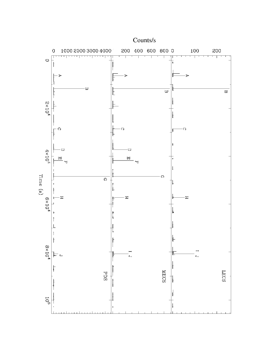
Figure 1: The X-ray light curves of the afterglow of SGR 1900+14  after the burst of 18 April 2001 in the LECS (upper panel), MECS (middle panel) and PDS (lower panel) energy ranges. The ten bursts considered in our spectral analysis are indicated by the letters from A to J.

The MECS (2–10 keV) light curve (Fig. 1 - middle panel) shows many short bursts, many having peak count rates more than two orders of magnitude above the persistent X-ray emission level from SGR 1900+14. In our analysis we considered only the events with an integral number of counts in the MECS band larger than 100, enough to obtain significant constraints on spectral fit parameters. Thus, we selected only ten bursts whose salient properties are given in Table 1. We searched the PDS data for bursts coincident in time with those detected in the MECS light curve and found significant emission for all ten. Five of the bursts in Table 1 were also detected in the LECS data, but the number of counts in the energy range useful for spectral analysis (0.1-4 keV) is small and does not further constrain the spectral fit even for the brightest event (burst B). Thus, we limited our study only to the MECS and PDS data, with an effective energy range between 1.5 and $\sim$100 keV.

The background counts in the MECS images within an annulus surrounding the source extraction circle (of equal area), were found to be less than unity over the bursts time intervals. Hence, no background subtraction was applied. PDS background spectra were accumulated from simultaneous data acquired by off-source detectors. Publicly available matrices were used for all the instruments. MECS and PDS spectra were binned in order to have a minimum number of 20 counts in each bin. We used xspec 11 for fitting the data. The parameter uncertainties correspond to $90$% confidence for a single parameter, i.e., $\Delta\chi^{2}=+2.7$. MECS and PDS spectra were simultaneously fitted leaving the normalization constant free to vary in the range 0.80–0.90, according to the prescription given by Fiore, Guainazzi and Grandi (1999).

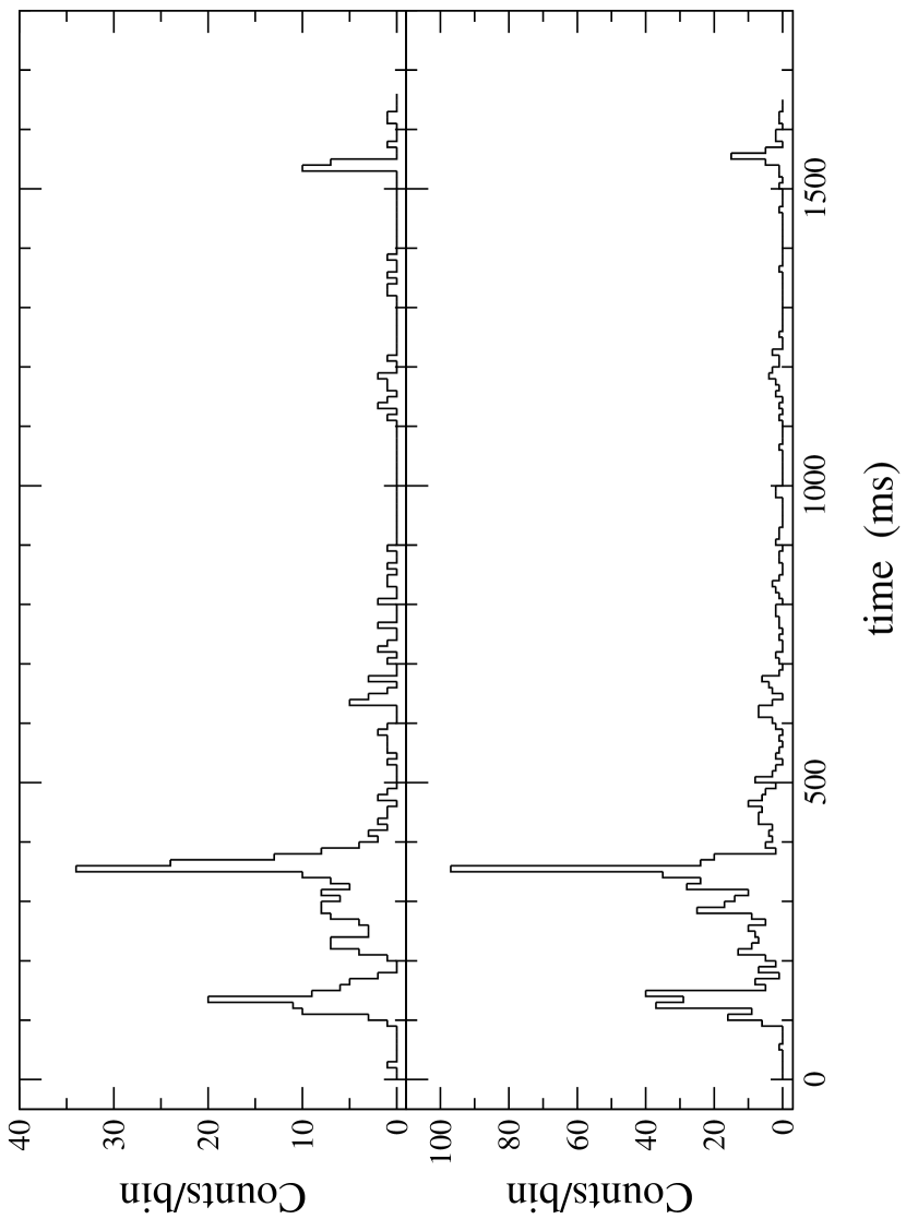
Figure 2: The X-ray light curves of the burst D in the MECS (upper panel) and PDS (lower panel) energy ranges, after correction for the different time off-set (see text for details). The time bin size is 10 ms.

The bursts are often characterized by the presence of several well separated peaks. When correlating the MECS and PDS light curves, we detected a systematic time delay of about 50 ms between the two instruments. This effect is possibly a consequence of the switch to the secondary clock onboard the BeppoSAX satellite in the year 2000. On the other hand, the similar time structure allowed for a post-facto empirical time re-alignment of the data, as shown in Fig. 2. Based on this assumption, the time-integrated energy spectra were extracted for the two instruments on time intervals encompassing valid simultaneous data from both instruments. We note that the two brightest bursts, B and G, had very strong initial spikes with high count rates (larger than 4,000 and 12,000 count/s in the MECS and PDS, respectively) that saturated the satellite telemetry, effectively truncating the light curves in the two instruments. We conservatively included in the spectral analysis only the counts safely away from the saturation edge.

3 BeppoSAX MECS and PDS Spectral Analysis

A critical parameter in the modeling of these SGR burst spectra is the column density of neutral absorbing gas along the line of sight. The most precise measurement of this parameter comes from modeling of the persistent X-ray emission. In quiescence, the X-ray spectrum of SGR 1900+14 is best fit (Woods et al. 1999) by the sum of a blackbody ($kT\simeq$ 0.5 keV) and a power law (photon index $\Gamma\simeq$ 1.0-2.5). For this model, the column density is consistently measured at N${}_{H}\simeq 2.5\times 10^{22}$ cm^-2 (Woods et al. 1999; Woods et al. 2001; Kouveliotou et al. 2001; Feroci et al. 2003). However, this particular observation where our bursts were recorded took place during a state of enhanced flux following the 2001 April 18 flare (Feroci et al. 2003), a so-called ‘afterglow state’. Fit to a simple power law, the $N_{\rm H}$  measured at this time is (4.41$\pm$0.25) $\times$ 10²² cm^-2. Although not statistically required by the data, the addition of a blackbody component to the power law model provides a good fit to the persistent X-ray emission at this time, with an $N_{\rm H}$ consistent with the quiescent state (but more loosely constrained), but with a temperature close to 1 keV (Mereghetti et al., in preparation). Indeed, similar variations of the blackbody temperature have been observed in this and other magnetar candidates (e.g., Lenters et al. 2003, Woods et al. 2004) following intense burst activity. Thus, it cannot be excluded that the $N_{\rm H}$ for SGR 1900+14  at the time of this observation might have been consistent with the quiescent value of $\sim 2.5\times$ 10²² cm^-2. Here, we will adopt a conservative approach and allow $N_{\rm H}$  to vary between 2 and 5 $\times 10^{22}$ cm^-2 for our spectral fits.

One important conclusion from our analysis is that the OTTB model fails to give acceptable fits to the spectral energy distributions of all bursts. Using the combined data set (MECS and PDS) for each burst and assuming $N_{\rm H}$ =2.5$\times$10²² cm^-2, the $\chi^{2}_{r}$  are all in the interval 2–7 (with 12 to 46 degrees of freedom - d.o.f.), while for $N_{\rm H}$ =4.4$\times$10²² cm^-2 the $\chi^{2}_{r}$  are lower but remain mostly statistically unacceptable ($\chi^{2}_{r}$  between 1.4 and 4.8, except for burst J for which $\chi^{2}_{r}$ =1.0, 22 d.o.f.). When we limit the fit to the PDS data only (E $>$ 15 keV) we generally obtain very good results (0.5$<$ $\chi^{2}_{r}$$<$ 1.2), with the exception of burst C ($\chi^{2}_{r}$=2.1). The measured temperatures ($kT$) are in the range 19–28 keV, in agreement with the values usually found for the short bursts in this energy range (e.g., Aptekar et al. 2001). To concisely show the inadequacy of the OTTB model over the full band, we show a fit to the sum of the spectra of all bursts (Average Spectrum, Top Panel of Fig. 3) with $N_{\rm H}$ fixed at the maximum value within our range, 5$\times$10²² cm^-2 ($\chi^{2}_{r}$  = 4.1 for 30 d.o.f.). If $N_{\rm H}$ is left free to vary, a marginally good fit is found ($\chi^{2}_{r}$ =1.22 for 29 d.o.f.), but with an unrealistic value of $N_{\rm H}$ (13.2${}^{+2.2}_{-2.0}$ $\times 10^{22}$ cm^-2, with kT=23.1${}^{+1.5}_{-1.4}$ keV). A back extrapolation of the fit to the PDS data only severely overestimates the observed flux at lower photon energies (Fig. 3, Bottom Panel). We conclude that the OTTB model fails to fit the broad-band burst spectra of SGR 1900+14.

Next, we attempted to find an acceptable model for the burst spectra that fits both the high and low energies. A single BB spectrum, which is characterized by a greater curvature, does not give acceptable best fits for either the individual or the Average BeppoSAX burst spectra ($\chi^{2}_{r}$  $>$ 2.8). Another possible thermal model is the sum of two BBs, as used by Olive et al. (2003) to fit the 7–150 keV FREGATE spectral data of the 2001 July 2 burst from this source. When applied either to the individual burst spectra or to the Average Spectrum it yields a statistically acceptable $\chi^{2}_{r}$. The best fit parameters are given in Table 2. The fit with this model to the Average Spectrum is shown in the upper panel of Figure 5. The dispersion of the two BB temperatures is small, consistent within statistics: for the low temperature BB we found a mean $<kT_{1}>$ value of 3.23 keV with a standard deviation of 0.56 keV, while the high temperature component has a mean $<kT_{2}>$=9.65 keV and a standard deviation of 0.95 keV. Such a narrow distribution of spectral parameters raises the question of whether the 10 bursts are all consistent with the same spectral parameters. We therefore performed a simultaneous fit to all the burst spectra linking the $N_{\rm H}$ , $kT_{1}$ and $kT_{2}$ between the individual bursts. The fit is satisfactory (line ”Joint Fit” in Table 2) with parameters consistent with those derived from the fit to the Average Spectrum, as well as with the mean of the parameters derived from the fits to the individual spectra. Interestingly, the ratio of the bolometric luminosities of the two BBs is approximately constant for the different bursts (Table 2 and Fig. 4). We note also that the best-fit parameters for the spectrum of the 2001 July 2 event obtained by Olive et al. (2003) using the same model are nicely consistent with our temperature distributions ($kT_{1}$=4.15 keV and $kT_{2}$=10.4 keV).

Finally, we also tested a cut-off power law model. The best-fit parameters for both individual and Average burst spectra are given in Table 3, for our restricted ranges of $N_{\rm H}$. The fit results are satisfactory, especially for larger $N_{\rm H}$ values near the maximum of our range. As was the case for the two BBs model, we note that the spectral parameters are rather clustered. The cut-off energy distribution is centered at $<E_{c}>$ = 15.8 keV, with a standard deviation of only 2.3 keV and the mean spectral index $<\Gamma>$ is 0.4, with a dispersion of 0.2. Also for this case, a joint fit of all the spectra with linked fit parameters (except for the normalizations) provided satisfactory results (line “Joint Fit” in Table 3), consistent with the results on the Average Spectrum, as well as with the mean of the values found in the individual fits.

4 Discussion

The common, short bursts from SGR 1900+14 are ordinarily detected by the wide field-of-view experiments typically working above 15-20 keV or more. This led to a good empirical description of their spectra using the OTTB model, however, often criticized as non-physical when applied in this context (e.g., Fenimore et al. 1994). We have now demonstrated for the short bursts from SGR 1900+14  that the OTTB law is not acceptable even at an empirical level when the energy spectrum is studied across a broader energy range. A similar result was obtained by Fenimore et al. (1994) for SGR 1806-20.

We tested three alternative spectral models, still on phenomenological grounds, following an approach of simplicity. A critical spectral parameter for all models is the neutral absorption column. Leaving $N_{\rm H}$  free, the OTTB model is marginally acceptable, but the column density required is much larger than what is found during the persistent X-ray emission seconds before and after the burst. As a conservative approach, we therefore decided to constrain in all our fits an equivalent hydrogen column in the range of what has been measured for the persistent source. With this assumption in mind, we found that our best-fit models are two BBs and a cut-off power law. We have no strong statistical or physical argument to support one or the other. However, we note that the goodness of the fits with the cut-off power-law model is more critically sensitive to the choice of $N_{\rm H}$ . In particular, as shown in Table 3, the fits to the burst spectra converge to the highest $N_{\rm H}$ values allowed in the range. Similar to the OTTB model, the $\chi^{2}_{r}$  increases as the $N_{\rm H}$ decreases. Should the $N_{\rm H}$ be constrained to small values from future measurements, this would possibly affect the validity of the cut-off power law as a spectral model for the bursts.

A striking property of both models is the clustering of the parameters governing the spectral shape (i.e. the temperatures of the two BB model, and $E_{c}$ and $\Gamma$ for the power law with an exponential cut-off). Consistent with previous studies, this shows the uniformity of the SGR burst spectra with varying burst intensities. Interestingly, for the two BB model, the luminosity emitted by the two components is consistent with a constant ratio, showing that both components scale in intensity for brighter bursts. As for the cut-off power law model, it has to be noted that the photon index obtained in all our fits is always significantly smaller than what is expected for an energy distribution of particles in thermal equilibrium ($\Gamma$=1).

It is very interesting to note that the short bursts from SGR 1806-20 also possess a similar spectral shape as the ones we analyzed here from SGR 1900+14. However, Fenimore et al. (1994) measure an average column density of 1.1$\times$10²⁴ cm^-2 using an OTTB model with $kT\sim$22 keV. This column density is almost an order of magnitude larger than the value we measure for SGR 1900+14 using the same model, with similar $kT$. Thus, it appears that the roll-over at low energies in SGR 1806$-$20 is more severe than it is for SGR 1900+14.

Although perhaps quantitatively different, the spectral similarities for SGR 1900+14  and SGR 1806-20 may reflect a universal emission mechanism for short bursts independent of the specific source. This assertion would need support from similar analysis of short bursts from the other SGR sources. It is worth noting that such a universality is already suggested in the mechanism for the emission of the giant flares (e.g., Mazets et al. 1999, Feroci et al. 2001) for the two cases known so far from SGR 0526-66 and SGR 1900+14.

Two conclusions that we can draw from our observations are: i) the spectral shape of the individual bursts remains stable independent of the brightness, duration and light curve complexity of the events; ii) although we have identified two spectral models that provide a good description of the data, it remains to be seen whether these models truly reflect the physics behind the emission mechanism. Currently, the are no detailed predictions on the spectra of SGR bursts. A discussion on the physical interpretation of our results is beyond the scope of this Letter and we defer it to a future work.

5 REFERENCES

• Aptekar, R., et al. 2001, ApJS, 137, 227

• Boella, G., et al. 1997, A$\&$AS, 122, 327

• Cline, T., Mazets, E. and Golenetskii, S. 1998, IAU Circ. 7002

• Fenimore, E.E., Laros, J.G., and Ulmer, A., 1994, ApJ, 432, 742

• Feroci, M., Frontera, F., Costa, E. et al. 1999, ApJ, 515, L9

• Feroci, M., Hurley, K., Duncan, R.C., and Thompson, C., 2001, ApJ, 549, 1021

• Feroci, M., Mereghetti, S., Woods, P. et al. 2003, ApJ, 596, 470

• Fiore, F., Guainazzi, M., and Grandi, P., 1999, ”Cookbook for BeppoSAX NFI Spectral Analysis”, available at ”http://www.asdc.asi.it”

• Guidorzi, C., et al., 2004, A&A, 416, 297

• Hurley, K., et al. 1996, ApJ, 463, L13

• Hurley, K., et al. 1999a, ApJ, 510, L107

• Hurley, K., Cline, T., Mazets, E. et al. 1999b, Nature, 397, 41

• Hurley, K., et al. 1999c, ApJ, 510, L111

• Kouveliotou, C. et al. 1993, Nature, 362, 728

• Kouveliotou, C. et al. 1998, IAU Circ. 6929

• Kouveliotou, C., Strohmayer, T.E., Hurley, K. et al. 1999, ApJ, 510, L115

• Kouveliotou, C. et al. 2001, ApJ, 558, L47

• Laros, J.G., et al. 1986, Nature, 322, 152

• Lenters, G.T. et al. 2003, ApJ, 587, 761

• Mazets, E.P., Golenetskii, S.V., Guriyan Yu.A. 1979, Sov. Astron. Lett., 5(6), 343

• Mazets, E.P., et al . 1999, Astron. Lett. 25(10), 635

• Murakami, T., et al. 1999, ApJ, 510, L119

• Olive, J-F., et al., 2003, in Proc. ”Gamma Ray Bursts and Afterglow Astronomy 2001”, G.R. Ricker and R.K. Vanderspeck eds., AIP 662, p. 82.

• Strohmayer, T.E., and Ibrahim, A., 1998, in Proc. ”4th Huntsville Symp. on Gamma Ray Bursts”, C.A. Meegan, R.D. Preece and T.M. Koshut eds., AIP 428, p. 947.

• Vasisht, G., Kulkarni, S.R., Frail, D.A., and Greiner, J., 1994, ApJ, 431, L35

• Woods, P.M., et al., 1999, ApJL, 518, L103

• Woods, P.M., Kouveliotou, C., Gögüs, E. et al., 2003, ApJ, 596, 464

• Woods, P.M., et al., 2004, ApJ, 605, 378

Table 1: Main characteristics of the ten selected bursts.

Burst	Time	LECS	MECS	PDS	T90	Integration	Peak Flux	Fluence
	UT	Counts	Counts	Counts	Duration	Time	13-100 keV	2-100 keV
	SOD	(Total/Net)	(Total/Net)	(Total/Net)	(s)	(ms)
A	60328	20	153/151	289/270	0.67	199.6	55.60	5.13
B	65801	73/36	$>$611/469	$>$1008/949	0.23	200.4	81.25	$>$17.95
C	82558	14	119/107	208/185	1.16	430.8	21.65	3.32
D	91223	N/A	293/284	621/607	1.45	682.3	45.71	10.63
E	95772	N/A	218/209	384/361	0.78	499.8	39.80	6.71
F	95794	N/A	339/337	707/680	0.14	250.1	80.11	12.42
G	102409	N/A	$>$359/317	$>$1363/782	0.08	100.0	$>$150.83	$>$13.20
H	111159	17	175/171	441/409	0.07	110.8	85.74	7.05
I	134665	13	158/156	325/298	0.18	271.0	47.57	5.82
J	134687	22	243/239	394/379	0.25	381.0	34.40	7.47

Table 2: Burst spectral parameters for the two-blackbody model.

Burst	$N_{\rm H}$	$kT_{1}$	R${}_{{}_{1}}\tablenotemark{b}$	$kT_{2}$	R${}_{{}_{2}}\tablenotemark{b}$	$\chi^{2}_{r}$/dof	$\chi^{2}_{r}$	$L_{1}/L{{}_{2}}$
	(1022 cm-2)	(keV)	(km)	(keV)	(km)		($N_{\rm H}$ =4$\times 10^{22}$ cm-2)
A	2.0	3.2${}^{+0.5}_{-0.5}$	13.7	9.3${}^{+1.9}_{-1.5}$	1.8	0.95/14	1.15	0.90$\pm{0.23}$
B	2.5	3.4${}^{+0.3}_{-0.2}$	23.5	9.9${}^{+0.9}_{-0.8}$	2.7	0.83/43	0.89	1.00$\pm{0.16}$
C	2.1	2.1${}^{+0.4}_{-0.5}$	13.5	7.9${}^{+0.9}_{-0.8}$	1.5	0.64/9	0.71	0.83$\pm{0.24}$
D	2.0	3.3${}^{+0.5}_{-0.5}$	9.9	10.2${}^{+1.5}_{-1.5}$	1.1	1.27/29	1.59	0.77$\pm{0.17}$
E	2.0	2.7${}^{+0.5}_{-0.4}$	12.2	8.6${}^{+0.9}_{-0.9}$	1.6	1.52/18	1.80	0.82$\pm{0.17}$
F	2.0	3.6${}^{+0.3}_{-0.5}$	16.5	10.3${}^{+1.1}_{-1.3}$	1.9	0.87/32	1.11	0.90$\pm{0.19}$
G	2.0	3.7${}^{+0.4}_{-0.3}$	24.4	8.9${}^{+0.7}_{-1.0}$	4.2	0.83/31	1.02	0.83$\pm{0.14}$
H	2.0	4.1${}^{+0.4}_{-0.8}$	15.7	10.5${}^{+2.2}_{-2.0}$	2.1	0.54/20	0.69	0.83$\pm{0.19}$
I	2.5	3.3${}^{+0.4}_{-0.5}$	11.9	11.0${}^{+1.8}_{-1.5}$	1.2	1.04/13	1.09	0.76$\pm{0.18}$
J	2.0	3.0${}^{+0.4}_{-0.4}$	13.9	9.9${}^{+1.3}_{-1.2}$	1.3	0.92/19	1.31	1.03$\pm{0.21}$
Average Spectrum	2.0	3.4${}^{+0.2}_{-0.3}$	13.4	9.33${}^{+0.8}_{-0.8}$	1.9	0.62/27	0.92	0.85$\pm{0.17}$
Joint Fit	2.0	3.34${}^{+0.13}_{-0.14}$	N/A	9.47${}^{+0.38}_{-0.39}$	N/A	1.02/255	1.19	N/A

Table 3: Burst spectral parameters for the cutoff-power law.

Burst	$N_{\rm H}$	$\Gamma$	$E_{c}$	$\chi^{2}_{r}$/dof				$N_{\rm H}$	$\Gamma$	$E_{c}$	$\chi^{2}_{r}$
	(1022 cm-2)		(keV)					(1022 cm-2)		keV
A	3.0	0.30${}^{+0.11}_{-0.32}$	14.9${}^{+3.0}_{-3.3}$	0.99/15				4.30	0.31${}^{+0.39}_{-0.20}$	14.6${}^{+4.7}_{-2.4}$	0.89
B	3.0	-0.01${}^{+0.23}_{-0.09}$	12.1${}^{+2.3}_{-0.9}$	1.60/44				5.0	0.28${}^{+0.26}_{-0.10}$	14.1${}^{+1.5}_{-2.2}$	1.3
C	3.0	0.44${}^{+0.25}_{-0.22}$	16.2${}^{+3.8}_{-4.0}$	1.05/10				4.0	0.43${}^{+0.43}_{-0.16}$	15.9${}^{+6.4}_{-2.9}$	1.06
D	3.0	0.38${}^{+0.19}_{-0.23}$	16.8${}^{+3.0}_{-2.0}$	0.97/30				4.08	0.51${}^{+0.09}_{-0.21}$	18.0${}^{+4.6}_{-2.3}$	0.93
E	2.85	0.25${}^{+0.29}_{-0.19}$	14.5${}^{+3.0}_{-1.0}$	1.44/19				4.0	0.27${}^{+0.47}_{-0.13}$	14.4${}^{+5.6}_{-1.2}$	1.48
F	3.0	0.22${}^{+0.16}_{-0.19}$	14.5${}^{+1.8}_{-2.2}$	1.00/33				5.0	0.50${}^{+0.09}_{-0.23}$	16.6${}^{+2.3}_{-3.2}$	0.88
G	3.0	0.004${}^{+0.10}_{-0.23}$	12.2${}^{+0.9}_{-2.2}$	1.01/32				4.27	0.04${}^{+0.08}_{-0.23}$	12.2${}^{+1.9}_{-1.3}$	0.94
H	3.0	0.14${}^{+0.09}_{-0.37}$	13.6${}^{+1.2}_{-3.3}$	0.81/22				5.0	0.25${}^{+0.10}_{-0.31}$	13.9${}^{+2.6}_{-3.0}$	0.68
I	3.0	0.43${}^{+0.14}_{-0.12}$	19.1${}^{+3.1}_{-5.9}$	1.77/14				5.0	0.46${}^{+0.34}_{-0.15}$	18.3${}^{+7.7}_{-2.7}$	1.37
J	3.0	0.58${}^{+0.12}_{-0.14}$	18.1${}^{+1.9}_{-3.8}$	0.87/20				4.63	0.72${}^{+0.19}_{-0.18}$	19.5${}^{+3.3}_{-4.2}$	0.81
Average Spectrum	3.0	0.17${}^{+0.18}_{-0.12}$	13.5${}^{+1.7}_{-1.2}$	1.13/28				5.0	0.42${}^{+0.12}_{-0.14}$	15.3${}^{+1.8}_{-1.6}$	0.82
Joint Fit	3.0	0.18${}^{+0.07}_{-0.06}$	13.9${}^{+0.7}_{-0.6}$	1.16/265				5.0	0.40${}^{+0.06}_{-0.07}$	15.5${}^{+0.8}_{-0.8}$	1.04

Figure 3: The best-fit OTTB model applied to the Average Spectrum of all the ten bursts, computed from MECS and PDS data (top panel) and from PDS data only (bottom panel).

Figure 4: Bolometric luminosity of BB2 (with higher kT) versus luminosity of BB1 (with smaller kT) for the ten bursts.

Figure 5: The best-fit for the power law with an exponential cutoff model (upper panel, with $N_{\rm H}$ =5$\times 10^{22}$ atoms cm^-2) and for the sum of two blackbodies (lower panel, with $N_{\rm H}$ =2$\times 10^{22}$ atoms cm^-2) for the Average Spectrum of all the ten bursts.