Using the filaments in the LCRS to test the $\Lambda$CDM model

Abstract

It has recently been established that the filaments seen in the Las Campanas Redshift Survey (LCRS) are statistically significant at scales as large as $70$ to $80\,h^{-1}{\rm Mpc}$ in the $\delta=-3^{\circ}$ slice, and $50$ to $70\,h^{-1}{\rm Mpc}$ in the five other LCRS slices. The ability to produce such filamentary features is an important test of any model for structure formation. We have tested the $\Lambda{\rm CDM}\,\,$model with a featureless, scale invariant primordial power spectrum by quantitatively comparing the filamentarity in simulated LCRS slices with the actual data. The filamentarity in an unbiased $\Lambda{\rm CDM}\,\,$model, we find, is less than the LCRS. Introducing a bias $b=1.15$, the model is in rough consistency with the data, though in two of the slices the filamentarity falls below the data at a low level of statistical significance. The filamentarity is very sensitive to the bias parameter and a high value $(b=1.5)$, which enhances filamentarity at small scales and suppresses it at large scales, is ruled out. A bump in the power spectrum at $k\sim 0.05\,h\,{\rm Mpc^{-1}}$ is found to have no noticeable effect on the filamentarity.

1 Introduction

Quantifying the clustering pattern observed in the galaxy distribution and explaining its origin has been one of the central themes in modern cosmology (eg. Peebles 1980). Traditionally, correlation functions have been used for this purpose, with the two-point correlation function $\xi(r)$ and its Fourier transform, the power spectrum $P(k)$, receiving most of the attention. There now exist precise estimates of $\xi(r)$ (eg. Tucker et al. 1997, LCRS; Hawkins et al. 2003, 2dFGRS; Zehavi et al. 2002 SDSS) and $P(k)$ (eg. Lin et al. 1996, LCRS ; Percival et al. 2001, 2dFGRS; Tegmark et al. 2003a, SDSS ) determined from several extensive redshift surveys. It is found that the large scale clustering of galaxies is well described by a featureless, adiabatic, scale invariant primordial power spectrum in a $\Lambda{\rm CDM}$ cosmological model. We shall, henceforth, refer to this combination of the background cosmological model and the power spectrum as the $\Lambda{\rm CDM}\,\,$model. The observed CMBR anisotropies (eg. Spergel et al. 2003, WMAP), and the joint analysis of CMBR anisotropies and galaxy clustering data (eg. Tegmark et al., 2003b), which place very precise constraints on cosmological models, are all consistent with the $\Lambda{\rm CDM}\,\,$model. This model is now generally accepted as the minimal model which is consistent with most currently available cosmological data.

One of the most striking visual features in all the galaxy redshift surveys e.g., CfA (Geller & Huchra 1989), LCRS (Shectman et al. 1996), 2dFGRS (Colless et al. 2001, Colless al. 2003) and SDSS (EDR) (Stoughton, et al. 2002, Abazajian et al. 2003). is that the galaxies appear to be distributed along filaments. These filaments are interconnected and form a network known as the “Cosmic Web”. The region in between the filaments are voids which are largely devoid of galaxies. This description of the galaxy distribution, based on the morphology of coherent structures observed in redshift surveys, addresses an aspect of the clustering pattern which is completely missed out by the two-point statistics like $\xi(r)$ and $P(k)$. In the currently accepted scenario of structure formation, the primordial density perturbations are a Gaussian random field which is completely described by the power spectrum, the phases of different modes being random. As structure formation progresses, coherent structures like sheets and filaments are formed through the process of gravitational instability. The phases of different Fourier modes are now correlated, and the power spectrum does not fully describe the statistical properties of the large scale structures. The full hierarchy of N-point statistics can, in principle, be used to quantify all properties of the large-scale structures, but these, being hard to determine at large scales, have not been perceived as the optimum tool for this purpose. Direct methods of quantifying the morphology and topology of large scale coherent features (as we discuss later) have been found to be more effective. The ability to produce large-scale coherent structures like the filaments observed in galaxy surveys is an important test of any models of structure formation. Any such test addresses issues beyond the scope of the two-point statistics like the power spectrum. In this paper we ask the question whether the $\Lambda{\rm CDM}\,\,$model is consistent with the filaments observed in galaxy redshift surveys.

The analysis of filamentary patterns in the galaxy distribution has a long history dating back to papers by Zel’dovich, Einasto and Shandarin (1982), Shandarin and Zel’dovich (1983) and Einasto et al. (1984) . In the last paper the authors analyze the distribution of galaxies in the Local Supercluster where they find filaments whose lengths increase with smoothing and finally get interconnected into an infinite network of superclusters and voids. The percolation analysis and the genus statistics (Zel’dovich et al. 1982; Shandarin & Zel’dovich 1983, Gott, Dickinson & Mellot 1986) were some of the earliest statistics introduced to quantify the network like topology of the galaxy distribution. A later study (Shandarin & Yess 2000) used percolation analysis to show the presence of a network like structure in the distribution of the LCRS galaxies. The large-scale and super large-scale structures in the distribution of the LCRS galaxies have also been studied by Doroshkevich et al. (2001) and Doroshkevich et al. (1996) who find evidence for a network of sheet like structures which surround underdense regions (voids) and are criss-crossed by filaments. The distribution of voids in the LCRS has been studied by Müller, Arbabi-Bidgoli, Einasto, & Tucker (2000) and the topology of the LCRS by Trac, Mitsouras, Hickson, & Brandenberger (2002) and Colley (1997). A recent analysis (Einasto et al. 2003) indicates a super cluster-void network in the Sloan Digital Sky Survey also. Colombi, Pogosyan and Souradeep (2001) have studied the topology of excursion sets at the percolation threshold. The minimal spanning tree (Barrow,Bhavsar & Sonoda 1985) is another useful way to probe the geometry of large scale structures. The morphology of superclusters in the PSCz has been studied by Basilakos, Plionis & Rowan-Robinson (2001) who find filamentarity to be the dominant feature. On comparing their results with the predictions of different cosmological models, they find that a low density $\Lambda$CDM model is preferred. These conclusions were further confirmed by Kolokotronis, Basilakos & Plionis (2002) using the Abell/ACO cluster catalogue.

The Minkowski functionals have been suggested as a novel tool to study the morphology of structures in the universe (Mecke et al. 1994; Schmalzing & Buchert 1997). Ratios of the Minkowski functionals can be used to define a shape diagnostic ’Shapefinders’ which faithfully quantifies the shapes of both simple and topologically complex objects (Sahni, Satyaprakash & Shandarin 1998). Bharadwaj et al. (2000) defined the Shapefinder statistics in two dimensions (2D), and used this to demonstrate that the galaxy distribution in the LCRS exhibits a high degree of filamentarity compared to a random Poisson distribution having the same geometry and selection effects as the survey. This analysis provides objective confirmation of the visual impression that the galaxies are distributed along filaments. In a later paper Bharadwaj, Bhavsar and Sheth (2004) used Shapefinders in conjunction with a statistical technique called Shuffle (Bhavsar & Ling 1988) to determine the maximum length-scale at which the filaments observed in the LCRS are statistically significant. They found that the largest length-scale at which filaments are statistically significant is between $70$ to $80\,h^{-1}$Mpc, for the LCRS $-3^{o}$ slice. Filamentary features longer than $80\,h^{-1}$Mpc, though identified, are not statistically significant. Such features arise from chance alignments of galaxies. Further, for the five other LCRS slices, filaments of lengths $50\,h^{-1}$Mpc to $70\,h^{-1}$Mpc were found to be statistically significant, but not beyond.

Comparing the filamentarity observed in galaxy redshift surveys against the predictions of different models of structure formation provides a unique method for testing these models. Here we present a method for carrying out this analysis in 2D, and as an example we apply it to the LCRS for which the filamentarity has already been extensively studied ( Bharadwaj et al. 2000; Bharadwaj et al. 2004). In this paper we address the question if the $\Lambda{\rm CDM}\,\,$model is consistent with the filaments observed in the LCRS. We have used cosmological N-body simulations to generate different realizations of the galaxy distribution one would expect in the LCRS for the $\Lambda{\rm CDM}$ model. The actual and simulated LCRS data were analyzed in exactly the same way using Shapefinders to quantify the degree of filamentarity, and the results were compared to test if the predictions of the $\Lambda{\rm CDM}$ model are consistent with the LCRS.

The LCRS galaxies may be a biased tracer of the underlying dark matter distribution whose evolution is followed by the N-body simulation. We also consider this possibility, and study how varying the bias parameter effects the network of filaments and voids.

Various independent lines of investigation seem to indicate that there may be excess power, in comparison to the $\Lambda{\rm CDM}\,\,$model, at scales $k\sim 0.05\,h\,{\rm Mpc}^{-1}$. The two dimensional power spectrum for the LCRS (Landy et al. 1996) exhibits strong excess power at wavelengths $\sim 100\,h^{-1}$Mpc. The analysis of the distribution of Abell clusters (Einasto et al. 1997a, 1997b) reveals a bump in the power spectrum at $k=0.05\,h\,{\rm Mpc}^{-1}$. Also, the recent analysis of the SDSS shows a bump in the power spectrum at nearly the same value of $k$ (Tegmark et al. 2003a). Such a bump would be a deviation from the $\Lambda{\rm CDM}\,\,$model and would be indicative of something very interesting happening at large scales. We have considered the possibility that there is such a bump in the power spectrum, and we investigated if the high level of filamentarity observed in the LCRS is indicative of excess power at $k=0.05\,h\,{\rm Mpc}^{-1}$ in the power spectrum.

To present a brief outline of our paper, in Section 2. we present the method of our analysis, in Section 3. we present our results and finally in Section 4. we discuss our results and present conclusions.

2 Method of analysis.

The LCRS has six slices, each $1.5^{o}$ thick in declination and $80^{o}$ wide in right ascension. Three of the slices are in the Northern galactic cap region centered around declinations $-3^{o}$, $-6^{o}$ and $-12^{o}$, and the other three are in the Southern galactic cap region at declinations $-39^{o}$, $-42^{o}$ and $-45^{o}$. We extracted volume limited subsamples with absolute magnitude limits $-21.5\leq M\leq-20.5$ so as to uniformly sample the region from $195$ to $375\,h^{-1}$Mpc in the radial direction. The subsamples used here and the method of analysis are exactly the same as in Bharadwaj et al. (2004).

Our data consist of a total of 5073 galaxies distributed in 6 slices. The slices were all collapsed along the thickness (in declination) resulting in a 2 dimensional truncated conical slice. Each slice was unrolled and then embedded in a $1\,h^{-1}{\rm Mpc}\times 1\,h^{-1}{\rm Mpc}$ 2D rectangular grid. Grid cells with galaxies in them were assigned the value 1, empty cells 0. Connected regions of filled cells were identified as clusters using a “friends-of-friends”(FOF) algorithm. The geometry and topology of a two dimensional cluster can be described by the three Minkowski functionals, namely its area $S$, perimeter $P$, and genus $G$. It is possible to quantify the shape of the cluster using a single 2D “Shapefinder” statistic (Bharadwaj et al. 2000) which is defined as the dimensionless ratio

$${\cal F}=\frac{P^{2}-4\pi S}{P^{2}+4\pi S}\,,$$ (1)

which by construction has values in the range $0\leq{\cal F}\leq 1$. It can be verified that ${\cal F}=1$ for an ideal filament which has a finite length and zero width, whereby it subtends no area ($S=0$) but has a finite perimeter ($P>0$). It can be further checked that ${\cal F}=0$ for a circular disk, and intermediate values of ${\cal F}$ quantifies the degree of filamentarity with the value increasing as a cluster is deformed from a circular disk to a thin filament.

The definition of ${\cal F}$ needs to be modified when working on a rectangular grid of spacing $l$. An ideal filament, represented on a grid, has the minimum possible width i.e. $l$, and its perimeter $P$ and area $S$ are related as $P=2S+2l$. At the other extreme we have $P^{2}=16S$ for a square shaped cluster on the grid. We introduce the 2D Shapefinder statistic

$${\cal F}=\frac{(P^{2}-16S)}{(P-4l)^{2}}$$ (2)

to quantify the shape of clusters on a grid. By definition 0$\leq{\cal F}\leq$ 1. ${\cal F}$ quantifies the degree of filamentarity of the cluster, with ${\cal F}$ = 1 indicating a filament and ${\cal F}$ = 0, a square, and ${\cal F}$ changes from $0$ to $1$ as a square is deformed to a filament.

Instead of studying the filamentarity of individual clusters, we use the average filamentarity to asses the morphological properties of the overall galaxy distribution. The average filamentarity $F_{2}$ is defined as the mean filamentarity of all the clusters in a slice weighted by the square of the area of each clusters

$$F_{2}={\sum_{i}{\cal S}_{i}^{2}{\cal F}_{i}\over\sum_{i}{\cal S}_{i}^{2}}\,.$$ (3)

The extent of filamentarity in a survey is strongly influenced by the morphology of its largest and most massive members. A supercluster will contribute more to the overall texture of large-scale structure than an individual cluster of galaxies, and we incorporate this by using the second area-weighted moment of the filamentarity. In the current analysis, we use the average filamentarity to quantify the degree of filamentarity in each of the LCRS slices.

The galaxy distribution in the LCRS slices is quite sparse, and the Filling Factor $FF$, defined as the fraction of filled cells, is very small ($FF\sim 0.01$). The clusters identified using FOF contain at most 2 or 3 filled cells, and these do not correspond to the long filaments visible in the LCRS slices. It is necessary to coarse-grain, or smoothen, the galaxy distribution before it is possible to objectively identify the large-scale coherent structures picked out by our eyes. The coarse-graining is achieved by successively filling cells that are immediate neighbors of already filled cells. The filled cells get fatter after every iteration of coarse-graining. This causes clusters to grow, first because of the growth of filled cells, and then by the merger of adjacent clusters as they overlap. At the initial stages of coarse-graining, the patterns which emerge from the distribution of 1s and 0s closely resembles the coherent structures seen in the galaxy distribution. As the coarse-graining proceeds, the clusters become very thick and fill up the entire region washing away any patterns. $FF$ increases from $FF\sim$ 0.01 to $FF=$ 1 as the coarse graining proceeds. So as not to limit ourselves to an arbitrarily chosen value of $FF$, we present our results showing the average filamentarity $F_{2}$ for the entire range of filling factor $FF$ (eg. Figure 2). We use the plots of average filamentarity as a function of the filling factor to asses the overall morphology of the large-scale structures at various levels of smoothing. It may also be noted that the length-scale associated with the structures increases with the filling factor, and we have a single connected structure which percolates through the entire survey region as $FF\rightarrow 1$.

The cosmological simulations were carried out using a Particle Mesh (PM) N-body code. A comoving volume $[409.6h^{-1}{\rm Mpc}]^{3}$ was simulated using $256^{3}$ particles on a $512^{3}$ mesh. The set of values $(\Omega_{m0},\Omega_{\Lambda 0},h)=(0.3,0.7,0.7)$ were used for the cosmological parameters, and we used a $\Lambda{\rm CDM}$ power spectrum characterized by a spectral index $n_{s}=1$ at large-scales and with a value $\Gamma=0.2$ for the shape parameter. The power spectrum was normalized to $\sigma_{8}=1.0$, consistent with the COBE data, which gives a good fit to the LCRS power spectrum. We have also run simulations using $\sigma_{8}=0.84$ which is more in keeping with the WMAP results. We find that the results for the filamentarity are not very sensitive to the normalization. There is practically no difference if we use any one of the two above values, so we report results only for $\sigma_{8}=1.0$.

The N-body simulation gives us the final distribution of dark matter particles for different random realizations of the initial density fluctuations. We have run the simulation for three different realizations of the initial density fluctuations. In order to extract galaxies corresponding to the LCRS, the observer was placed at a suitable position in the N-body simulation cube and the dark matter peculiar velocities were used to take whole distribution over to redshift space. For each volume limited LCRS slice we identified a region in the N-body simulation which has exactly the same shape and size as the LCRS slice that we analyzed, and we extracted exactly the same number of dark matter particles as there are galaxies in the slice. For each LCRS slice we extracted three independent simulated slices located at three different orientations within a single N-body cube. This, combined with the three independent realizations of the initial density fluctuations, gives us nine independent simulations of each LCRS slice. These simulated slices, extracted from the N-body simulation were analyzed in exactly the same manner as the actual LCRS data.

Various lines of investigation indicate that galaxies may be a biased tracer of the underlying dark-matter distribution (eg. Peacock &Dodds 1994). Theoretical considerations (eg. Kauffmann et al. 1996, Scherrer & Weinberg 1998) also suggest that constant linear biasing holds on the large scales of interest here. We adopted the “sharp cutoff” scheme (Cole et al. 1998), a local biasing scheme where the probability of a mass particle being selected as a galaxy is a function of the neighbouring density field alone. In this scheme the final dark-matter distribution generated by the N-body simulation was first smoothened with a Gaussian of width 5 $h^{-1}$ Mpc. Only particles which lie in regions where the density contrast, in units of the rms. density fluctuation, exceeds a critical value were chosen. Varying the value of the critical density contrast changes the bias. We chose the values for the critical density contrast so as to produce particle distributions with a modest bias $b=1.15$ and high bias $b=1.5$. The simulated LCRS slices were extracted from the biased particle distribution in exactly the same manner as described for the unbiased case.

We have run three independent realizations of the N-body simulation for a model where the power spectrum has excess power at scales $k\sim 0.05\,h\,{\rm Mpc}^{-1}$. In these simulations the power at scales between $0.04\,h\,{\rm Mpc}^{-1}$ to $0.06\,h\,{\rm Mpc}^{-1}$ was increased by $100\%$, thereby introducing a bump in the power spectrum centered at $k=0.05\,h\,{\rm Mpc}^{-1}$. The simulated LCRS slices were extracted in exactly the same way as described earlier.

3 Results

We first show, in Figure 1, the galaxy distribution in one of the LCRS slices ($\delta=-3^{\circ}$) along with simulated slices for the $\Lambda{\rm CDM}\,\,$model, the $\Lambda{\rm CDM}\,\,$model with a high bias ($b=1.5$) and the $\Lambda{\rm CDM}\,\,$model with a bump. Comparing the simulated $\Lambda{\rm CDM}\,\,$slices with and without the bump shows that the bump does not seem to make any difference in the coherent structures, at least as far as the eye can make out. Introducing bias, we find, makes a difference. In the biased slice the galaxies are preferentially chosen from the dense regions which appear to be much more pronounced. Most of the galaxies being located in the very dense regions, the voids are larger and the biased slice seems to lack some of the very large scale coherent structures seen in the unbiased $\Lambda{\rm CDM}\,\,$slice. Visually comparing the actual LCRS with the simulated slices shows that $\Lambda{\rm CDM}\,\,$seems to reproduce the large-scale coherent features reasonably well. The galaxy distribution in the simulated $\Lambda{\rm CDM}\,\,$slice appears to be a little more diffuse in comparison to the actual slice, possibly indicating a small amount of bias.

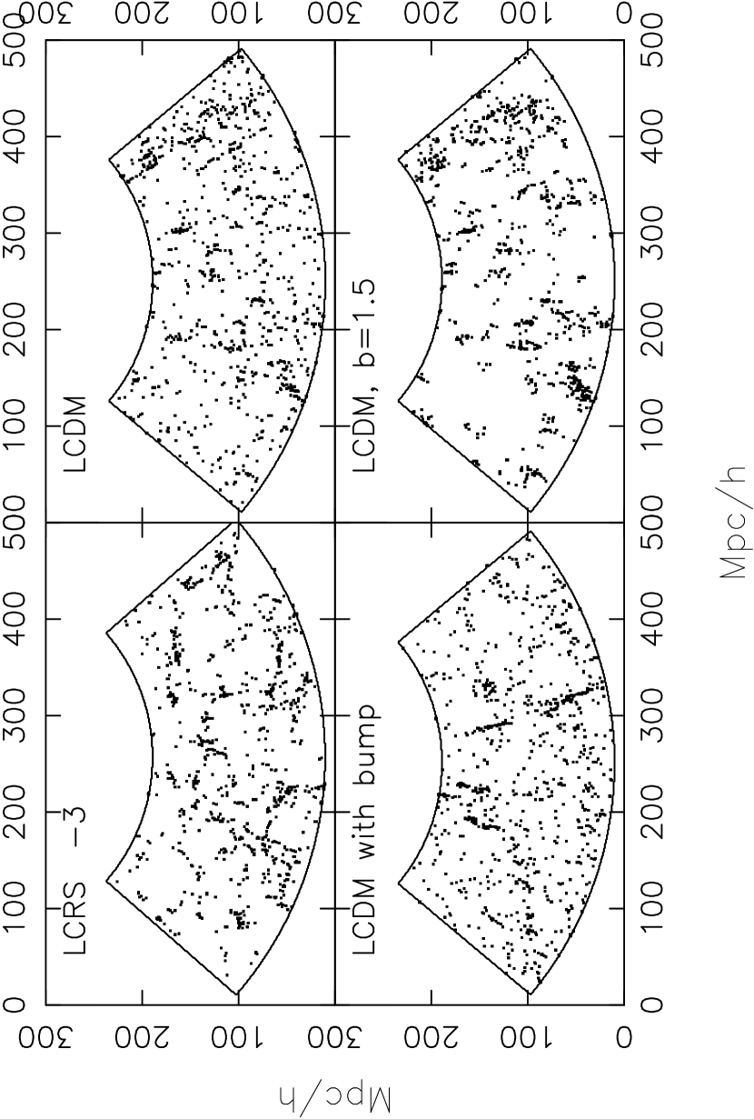
Figure 1: This shows the galaxy distribution in the LCRS slice at declination $\delta=-3^{\circ}$, along with the simulated slices as indicated in the panels. These figures show the galaxy distribution after it has been converted to a set of 1s and 0s on a grid, and after we have applied two iterations of the coarse-graining procedure described in Section 2. This, to some extent, enhances for our eyes the large scale coherent structures present in the galaxy distribution.

The results of our quantitative analysis of filamentarity using Shapefinders are shown in Figures 2 and 3. For each simulated slice we have used nine independent realizations to estimate the mean and the variance for the average filamentarity $F_{2}$ as a function of the filling factor $FF$. Earlier investigations (Bharadwaj et al. 2004) showed that the large-scale features are washed out at the level of coarse-graining where $FF\sim 0.7$, so we restricted our analysis to the range $FF\leq 0.7$ only. We used $\chi^{2}/\nu$ the reduced $\chi^{2}$ per degree of freedom (Table I) to quantify the deviations in the average filamentarity between the models and the actual LCRS slices.

We find that the average filamentarity in the unbiased $\Lambda{\rm CDM}\,\,$model is somewhat lower than the actual values for most of the slices (Figure 2). Introducing a small bias $(b=1.15)$ increases the average filamentarity at low filling factors, leaving the values at large filling factors unaffected. The fit to the actual data, as quantified by the values of $\chi^{2}/\nu$, shows a considerable improvement. Two of the slices ($\delta=-3^{\circ},-45^{\circ}$) have values of $\chi^{2}/\nu$ in the range $1.7$ to $1.8$, and it is less than $1.1$ for all the other slices. Given the lack of knowledge about the statistical properties of the errors in $F_{2}$, we may consider these values of $\chi^{2}/\nu$ as indicative of a reasonable agreement between this model ($\Lambda{\rm CDM}\,\,$,$b=1.15$) and the actual data. A large bias ($b=1.5$) changes the overall shape of the average filamentarity versus filling factor curves. With increasing bias, the average filamentarity goes up at small filling factors and it falls at large filling factors. Relating the filling factor to the size of the structures, we find that bias enhances filamentarity on small scales and suppresses the large-scale filamentary patterns. This is in keeping with the visual impression discussed earlier.

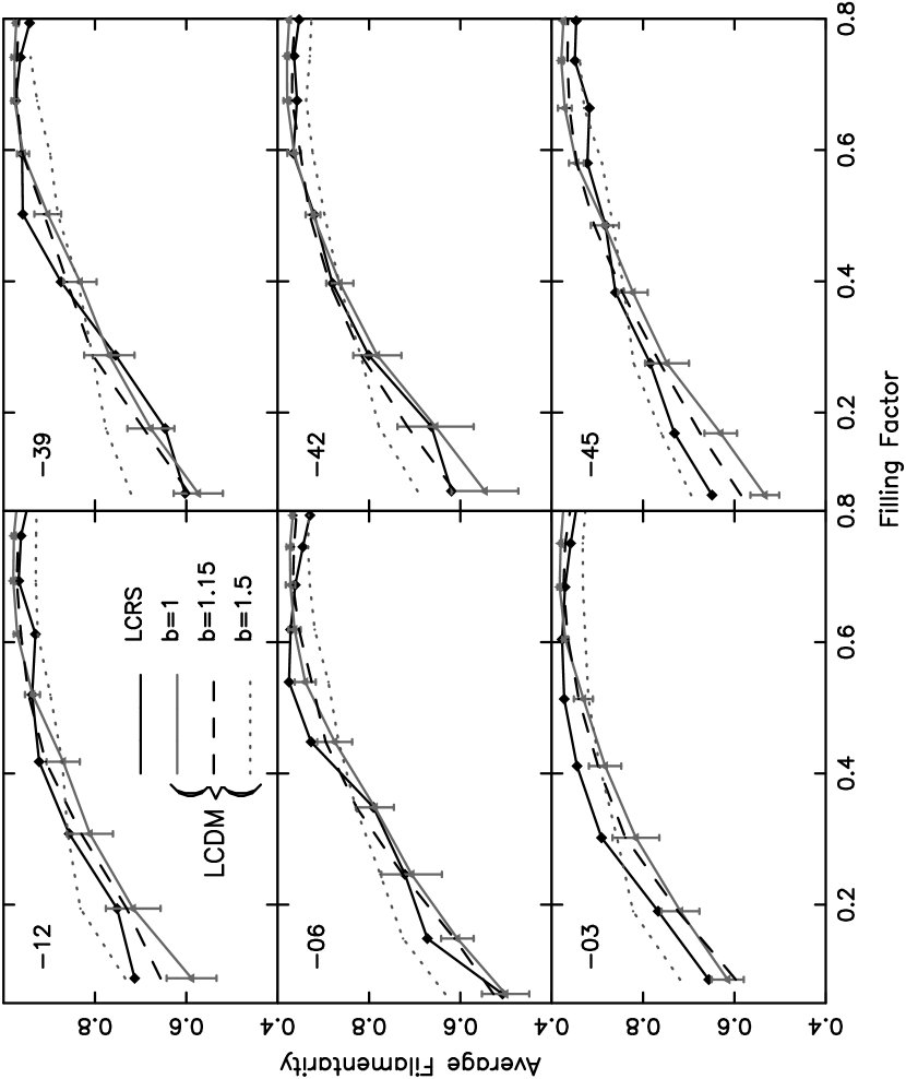
Figure 2: This shows the average filamentarity as a function of the filling factor for the six LCRS slices along with the results for the slices simulated in the $\Lambda{\rm CDM}\,\,$model with the different values of bias shown in the figure. Nine independent realizations of each of the simulated slices were used to calculate the mean and variance of the average filamentarity. The $1-\sigma$ error-bars are shown only for the unbiased $\Lambda{\rm CDM}\,\,$, the error-bars are similar for the biased models.

The results for the simulations using a $\Lambda{\rm CDM}\,\,$model with a bump are shown in Figure 3. Introducing a bump in the power spectrum does not seem to make a noticeable change in the average filamentarity. This is further reinforced by the values of $\chi^{2}/\nu$ which are very similar to the values when there is no bump.

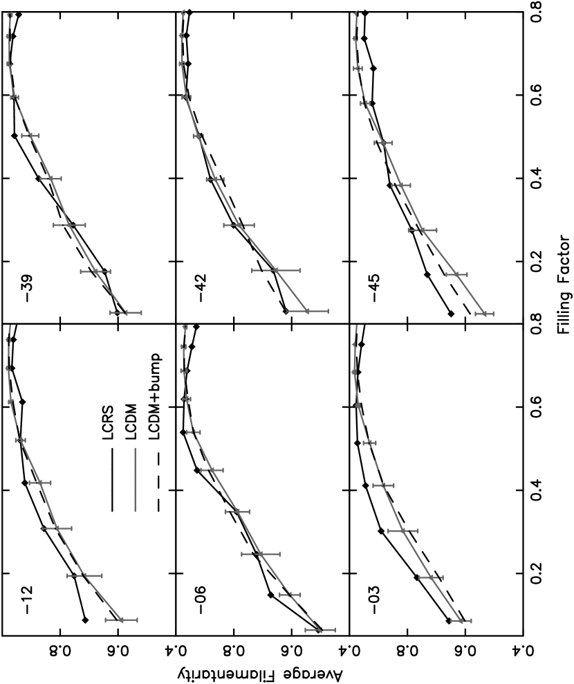
Figure 3: This shows the average filamentarity as a function of the filling factor for the six LCRS slices along with the results for the slices simulated in the $\Lambda{\rm CDM}\,\,$model with and without the bump. The $1-\sigma$ error-bars, shown only for the case without a bump, have similar values when a bump is introduced.

Table 1: For the LCRS slices at different declinations $\delta$, we tabulate below the values of $\chi^{2}/\nu$ for the $\Lambda{\rm CDM}\,\,$model with different values of bias and with a bump in the power spectrum.

$\delta$	$b=1$	$b=1.15$	$b=1.5$	Bump
$-3$	2.7	1.7	3.0	2.9
$-6$	1.8	1.1	4.3	1.2
$-12$	5.7	1.1	1.5	3.8
$-39$	0.89	0.80	5.7	0.77
$-42$	1.26	0.42	1.2	0.50
$-45$	5.5	1.8	1.0	2.7

4 Discussion and Conclusions

The $\Lambda{\rm CDM}\,\,$model has been found to be consistent with very precise observations of large-scale structures in the universe and their imprint on the CMBR. These tests are limited by the fact that most of them are based on two-point statistics which are not sensitive to the large-scale coherent features like the long filamentary patterns seen in galaxy redshift surveys. It has recently been established, for the LCRS, that the filaments are statistically significant to scale as large as $70$ to $80\,h^{-1}\,{\rm Mpc}$ (Bharadwaj et al 2004). In this paper we have tested whether the $\Lambda{\rm CDM}\,\,$model is consistent with the high level of filamentarity observed in the LCRS. A point to note is that the analysis presented here is restricted to two dimensional sections, and structures which appear as filaments could actually be sections of three dimensional planar structures. This issue whether the 2D filaments are actually also filaments in 3D, though not of crucial importance in the present discussion, is an interesting question which we plan to address in later work.

The filamentarity in the unbiased $\Lambda{\rm CDM}\,\,$model is lower than in the LCRS. Introducing a positive bias increases the filamentarity at small scales and suppresses the filamentarity at large scales. As the bias is increased, the galaxy distribution gets more concentrated in the high density regions, and the very large scale structures are suppressed. The values of the average filamentarity as a function of the filling factor (Figure 2) are sensitive to the bias, and the quantitative analysis of filamentarity holds the possibility of being a sensitive probe of the bias parameter. We have used two values of the bias parameter and find that a large bias $(b=1.5)$ is ruled out. The simulations with a smaller value of bias $(b=1.15)$ give a good fit to most of the LCRS slices, though in two of the slices ($\delta=-3^{\circ},\,-45^{\circ}$) the average filamentarity in the simulations falls somewhat below the LCRS for nearly the entire range of filling factor. The statistical significance of this mild discrepancy ($\chi^{2}/\nu\sim 1.8$) is not straightforward to interpret, and we adopt the point of view that the $\Lambda{\rm CDM}\,\,$model with a small bias is consistent with the filamentarity in the LCRS slices. It is interesting to note that the LCRS $\delta=-3^{\circ}$ slice, where the filamentarity is somewhat in excess of the biased $\Lambda{\rm CDM}\,\,$model, also has statistically significant filaments extending to scales ($70-80\,h^{-1}\,{\rm Mpc}$) larger compared to the other slices ($50-70\,h^{-1}\,{\rm Mpc}$) (Bharadwaj et al 2004). Analysis of the filamentarity in larger redshift surveys and a better understanding of the statistical properties of the errors in the average filamentarity will, in the future, allow this test to impose more stringent constraints on models of structure formation. A point to note is that the values of bias $b=1.15$ and $1.5$ have no special significance, and have been chosen as two convenient values one representing a modest bias and another a high bias. The value $b=1.15$ is consistent with the analysis of the LCRS power spectrum (Lin et al. 1996) who conclude that the value of the bias in the LCRS is in the range $0.7$ to $1.3$. A point to keep in mind is that the volume limited subsamples analyzed here contain only the very bright galaxies, and the bias is known to increase with the intrinsic luminosity of the galaxies (eg. Wild et al. 2004)

There have been speculations that there may be a bump in the power spectrum around the wave number $k\sim 0.05\,h\,{\rm Mpc^{-1}}$, and this may have an influence on the filamentary pattern seen in galaxy redshift surveys. We have considered a bump in the power spectrum which enhances the power in the range $0.04$ to $0.06\,h\,{\rm Mpc^{-1}}$, and we find that this does not have a significant influence on the average filamentarity at any value of the filling factor. The bump in the power spectrum, if it exists, seems to be unrelated to the filamentary patterns seen in redshift surveys.

It is interesting to compare our results with some of the other tests which probe models of structure formation beyond the two-point statistics. The bispectrum goes one step beyond the power spectrum, and is sensitive to non-Gaussian features. It has been used to test non-Gaussianity in the primordial power spectrum and determine the bias parameter (eg. Verde at al. 2002, Scoccimarro et al. 2001), but it does not tell us very much about individual, coherent features like filaments. The genus statistics quantifies the topology of the galaxy distribution. Studies of the 2D genus curve for the 2dFGRS (Hoyle et. al 2002a) and the SDSS (Hoyle et. al 2002b) are consistent with the predictions of the $\Lambda{\rm CDM}\,\,$model. Schmalzing and Diaferio (2000) have calculated the Minkowski functionals of the galaxy distribution in the nearby universe (the Updated Zwicky Catalogue) and they compare this with $\Lambda{\rm CDM}\,\,$N-body simulations. They find that galaxy distribution in the simulated distributions is less coherent than what is observed. Sheth et al. (2003) have developed a method called “Surfgen” for generating triangulated surfaces from a discrete galaxy distribution, and have used this to calculate the 3D Shapefinders. They have applied this to a variety of simulated data (Shandarin, Sheth and Sahni 2003, Sheth 2003), but results are awaited from real redshift surveys.

In conclusion we note the large-scale coherent features seen in galaxy redshift surveys provides a unique testing ground for probing the models of structure formation beyond the two-point statistics. These tests are also sensitive to the bias and hold the possibility of giving accurate estimates of the bias parameter. The analysis reported in this paper shows the $\Lambda{\rm CDM}\,\,$model with a modest bias to be roughly consistent with the filaments observed in the LCRS. Future work using large redshift surveys like the 2dFGRS and the SDSS should be able to accurately quantify the network of large scale coherent structures and place stringent limits on models of structure formation, taking precision cosmology into new grounds beyond the realm of two point statistics.

5 Acknowledgment

The authors wish to thank the LCRS team for making the survey data public. SB would like to acknowledge financial support from the Govt. of India, Department of Science and Technology (SP/S2/K-05/2001). BP would like to thank the CSIR, Govt. of India for financial support through a JRF fellowship.

References

- (1) Abazajian, K., Adelman-McCarthy, J.K., Agueros, M.A., Allam, S.S. & the SDSS Collaboration, 2003, astro-ph/0305492
- (2) Barrow, J. D., Bhavsar, S. P., & Sonoda, D. H. 1985, MNRAS, 216, 17
- (3) Basilakos,S., Plionis, M. & Rowan-Robinson,M., 2001, MNRAS, 323, 47
- (4) Bharadwaj, S., Sahni, V., Sathyaprakash, B. S., Shandarin, S. F. & Yess, C., 2000, ApJ, 528, 21
- (5) Bharadwaj, S., Bhavsar, S. P., & Sheth, J. V. 2004, ApJ, 606, 25
- (6) Bhavsar, S. P., Ling, E. N. 1988, ApJL, 331, 63
- (7) Cole, S., Hatton, S., Weinberg, D. H., & Frenk, C. S. 1998, MNRAS, 300, 945
- (8) Colless, M. et al. (for 2dFGRS team) 2001, MNRAS, 328, 1039
- (9) Colless et al. (for 2dFGRS team) 2003 astro-ph/0306581
- (10) Colley, W. N. 1997, ApJ, 489, 471
- (11) Colombi, S., Pogosyan, D. & Souradeep T. 2000, PRL, 85, 5515
- (12) Doroshkevich, A. G., Tucker, D. L., Fong, R., Turchaninov, V., & Lin, H. 2001, MNRAS, 322, 369
- (13) Doroshkevich, A. G., Tucker, D. L., Oemler, A. J., Kirshner, R. P., Lin, H., Shectman, S. A., Landy, S. D., & Fong, R. 1996, MNRAS, 283, 1281
- (14) Einasto, J., Hütsi, G., Einasto, M., Saar, E., Tucker, D. L., Müller, V., Heinämäki, P., Allam, S.S., 2003, A&A, 405, 425
- (15) Einasto, J. et al. 1997a, Nature, 385, 139
- (16) Einasto, M., Tago, E., Jaaniste, J., Einasto, J., & Andernach, H. 1997b, A&AS, 123, 119
- (17) Einasto, J., Klypin, A. A., Saar, E., & Shandarin, S. F. 1984, MNRAS, 206, 529
- (18) Geller, M. J. & Huchra, J. P. 1989, Science, 246, 897
- (19) Gott, J.R., Dickinson, M. & Mellot, A.L. 1986,ApJ,306,341
- (20) Hawkins, E., et al.,2003, MNRAS,346,78
- (21) Hoyle, F., Vogeley, M. S., & Gott, J. R. I. 2002a, ApJ, 570, 44
- (22) Hoyle, F., et al. 2002b, ApJ, 580, 663
- (23) Kauffmann, G., Nusser, A., & Steinmetz, M. 1997, MNRAS, 286, 795
- (24) Kolokotronis, V., Basilakos, S. & Plionis, M., 2002, MNRAS,331, 1020
- (25) Landy, S. D., Shectman, S. A., Lin, H., Kirshner, R. P., Oemler, A. , & Tucker, D. L. 1996, ApJL, 456, 1
- (26) Lin, H., Kirshner, R. P., Shectman, S. A., Landy, S. D., Oemler, A., Tucker, D. L., & Schechter, P. L. 1996, ApJ, 471, 617
- (27) Müller, V., Arbabi-Bidgoli, S., Einasto, J., & Tucker, D. 2000, MNRAS, 318, 280
- (28) Mecke, K. R., Buchert, T., & Wagner, H. 1994, A&A, 288, 697
- (29) Percival, W. J., et al. 2001, MNRAS, 327, 1297
- (30) Peacock, J. A. & Dodds, S. J. 1994, MNRAS, 267, 1020
- (31) Peebles, P. J. E., , Princeton University Press, The large-scale structure of the universe, Princeton University Press, 1980
- (32) Sahni, V., Sathyaprakash, B. S., & Shandarin, S.F. 1998, ApJL, 495, 5
- (33) Sathyaprakash, B.S., Sahni, V., Shandarin, S.F., & Fisher, K.B. 1998, ApJL, 507, 109
- (34) Scherrer, R. J. & Weinberg, D. H. 1998, ApJ, 504, 607
- (35) Schmalzing, J. & Buchert, T. 1997, ApJ, 482, L1
- (36) Schmalzing, J. & Diaferio, A. 2000, MNRAS, 312, 638
- (37) Scoccimarro, R., Feldman, H.A., Fry, J.N. & Frieman, J.A. 2001, ApJ,546,652
- (38) Shandarin, S. F. & Zel’dovich, I. B. 1983, Comments on Astrophysics, 10, 33
- (39) Shandarin, S. F. & Yess, C. 1998, ApJ, 505, 12
- (40) Shandarin,S.F., Sheth, J.V. & Sahni, V. 2003, (preprint astro-ph/0312110)
- (41) Shectman, S. A., et al., 1996, ApJ, 470, 172
- (42) Sheth, J.V. 2003, MNRAS, Submitted, (preprint astro-ph/0310755)
- (43) Sheth, J.V., Sahni, V., Shandarin, S.F., Sathyaprakash, B.S., 2003, MNRAS, 343, 22
- (44) Spergel, D. N. et al. 2003, ApJS, 148, 175
- (45) Stoughton, C. et al. (for the SDSS collaboration), 2002, AJ, 123, 485
- (46) Tucker, D. L., et al., 1997, MNRAS, 285, 5
- (47) Zel’dovich, Ya. B., 1970, A&A, 5, 84
- (48) Tegmark, M., et al., 2003a, ApJ, Submitted (astro-ph/0310725)
- (49) Tegmark, M., et al., 2003b, ApJ, Submitted (astro-ph/0310723)
- (50) Trac, H., Mitsouras, D., Hickson, P., & Brandenberger, R. 2002, MNRAS, 330, 531
- (51) Verde, L., et al. 2002, MNRAS,335,432
- (52) Wild et al. 2004,MNRAS, Submitted, (astro-ph/0404275)
- (53) Zehavi, I., et al. 2002, ApJ,571,172
- (54) Zel’dovich, I. B., Einasto, J., & Shandarin, S. F. 1982, Nature, 300, 407