The K20 survey. VI. The Distribution of the Stellar Masses in Galaxies up to $z\simeq 2$.

We present a detailed analysis of the stellar mass content of galaxies up to $z=2.5$ as obtained from the K20 spectrophotometric galaxy sample. We have applied and compared two different methods to estimate the stellar mass $M_{*}$ from broad–band photometry: a Maximal Age approach, where we maximize the age of the stellar population to obtain the maximal mass compatible with the observed $R-K$ color, and a Best Fit model, where the best–fitting spectrum to the complete $UBVRIzJK_{s}$ multicolor distribution is used. We find that the $M_{*}/L$   ratio decreases with redshift: in particular, the average $M_{*}/L$ ratio of early type galaxies decreases with $z$, with a scatter that is indicative of a range of star–formation time-scales and redshift of formation. More important, the typical $M_{*}/L$   ratio of massive early type galaxies is larger than that of less massive ones, suggesting that their stellar population formed at higher $z$. We show that the final K20 galaxy sample spans a range of stellar masses from $M_{*}=10^{9}M_{\odot}$ to $M_{*}=10^{12}M_{\odot}$: massive galaxies ($M_{*}\geq 10^{11}M_{\odot}$) are common at $0.5<z<1$, and are detected also up to $z\simeq 2$. We compute the Galaxy Stellar Mass Function at various z, of which we observe only a mild evolution (i.e. by 20-30%) up to $z\simeq 1$. At $z>1$, the evolution in the normalization of the GSMF appears to be much faster: at $z\simeq 2$, about 35% of the present day stellar mass in objects with $M_{*}\simeq 10^{11}M_{\odot}$ appear to have assembled. We also detect a change in the physical nature of the most massive galaxies: at $z\lower 2.15277pt\hbox{$\;\buildrel<\over{\sim}\;$}0.7$, all galaxies with $M>10^{11}M_{\odot}$ are early type, while at higher $z$ a population of massive star–forming galaxies progressively appears. We finally analyze our results in the framework of $\Lambda$–CDM hierarchical models. First, we show that the large number of massive galaxies detected at high $z$ does not violate any fundamental $\Lambda$–CDM constraint based on the number of massive DM halos. Then, we compare our results with the predictions of several renditions of both semianalytic as well as hydro-dynamical models. The predictions from these models range from severe underestimates to slight overestimates of the observed mass density at $\leq 2$. We discuss how the differences among these models are due to the different implementation of the main physical processes.

1 Introduction

The recent consolidation of the “concordance” cosmological scenario (Bennett et al. 2003), where several independent observational evidences have provided precise measures for the basic cosmological parameters, is opening a unique opportunity to understand the processes that led to galaxy formation and evolution. Without much residual ambiguity about the redshift-cosmic time relation and the dark energy/dark matter content of the universe, observations of galaxies at low and high redshift can better shed light on such processes as a function of both cosmological time and local over-density.

In the “concordance” cosmological scenario, the history of galaxies is driven by the build-up of the stellar population contained in their dark matter halos. Hierarchical theories of galaxy formation are characterized by a gradual enrichment of the star content of galaxies as a result of gas cooling within dark matter halos, and of progressive growth of the galaxy mass through merging events which may also promote massive star-bursts. However, different renditions of the hierarchical paradigm can differ dramatically in their predictions. In some cases an extremely rapid decrease of the number density of massive galaxies with increasing redshift is predicted (e.g., Baugh et al. 2003), while in other cases such decrease does not start until beyond $z\sim 1$ (e.g., Nagamine et al. 2001a,b; Hernquist & Springel 2003; Somerville et al. 2004a, Nagamine et al. 2004). Clearly, the direct mapping of galaxy evolution through cosmic time can effectively restrict the choice among such models.

Within this framework, $K$–band surveys have long been recognized as ideal tools to study the process of mass assembly at high redshift (Broadhurst et al. 1992, Gavazzi et al. 1996; Madau, Pozzetti & Dickinson 1998). With respect to optical bands, indeed, the $K$ band samples up to high $z$ the rest frame optical and near–IR spectral range, and therefore it is less sensitive to the instantaneous star formation activity and to dust extinction. Albeit the relation between near–IR luminosity and stellar mass is not univocal, deep imaging and spectroscopic surveys have been carried on to test the cosmological scenarios on mass–selected galaxy samples (Songalia et al. 1994; Kauffmann & Charlot 1998; Fontana et al. 1999; Cohen et al. 1999; Drory et al. (2001); Firth et al. 2002).

The K20 survey (Cimatti et al. 2002a) has been designed to extend and complement these studies, with the explicit aim of investigating the high redshift evolution of massive galaxies. It is based on a sample of about 500 galaxies to $K_{s}<20$, for which a nearly complete spectroscopic identification and a deep $UBVRIzJK_{s}$ multicolor coverage is available, which together make it an ideal dataset to study the evolution of a mass-selected sample of galaxies up to $z\simeq 2$. In the K20 dataset, the evolution of bright, massive galaxies has been investigated up to $z\simeq 2$ through the study of the $K$–limited redshift distribution (Cimatti et al. 2002b) and the near–IR luminosity functions (Pozzetti et al. (2003)). The results of the K20 survey show that galaxies selected in the $K$ band are characterized by a modest luminosity evolution up to $z\simeq 1$, that seems well described by simple pure luminosity evolution (PLE) models.

In this paper, we will use the K20 dataset to directly study the evolution of the stellar mass content in galaxies up to $z\simeq 2$. Recently, various techniques have been developed to directly estimate the stellar mass content of galaxies up to $z\sim 3$. Some rely on detailed spectral analysis (Kauffmann et al. 2003, for low $z$ galaxies), others on multi-wavelength imaging observations to remove or reduce the uncertainties involved in the conversion between near–IR luminosity and stellar mass (Giallongo et al. 1998; Brinchmann & Ellis 2000; Cole et al. 2001; Papovich et al. 2001; Shapley et al. 2001; Drory et al. 2001; Dickinson et al. 2003 - D03 hereafter-; Fontana et al. 2003 - F03 hereafter-; Rudnick et al. 2003; Saracco et al. 2004).

The applications of such techniques have been primarily driven by the available datasets. On a relatively shallow dataset, Giallongo et al. (1998) emphasized that at $z\simeq 0.7$ blue “faint” galaxies are an order of magnitude less massive than redder galaxies of comparable $B$ magnitude, and attempted a first estimate of the evolution of the cosmological mass density up to high $z$. Brinchmann & Ellis (2000) used a multi-wavelength coverage of the CFRS galaxy sample (Lilly et al. 1995) to trace the stellar mass density in morphologically selected galaxy samples up to $z=1$, while Drory et al. (2001) used a larger set of galaxies with photometric redshifts to set an upper limit on their mass density at $z\simeq 1$. Papovich et al. (2001) and Shapley et al. (2001) pushed this technique to its limit to constrain the mass of Lyman–break galaxies, showing that objects with stellar mass in excess of $10^{10}M_{\odot}$ are commonly detected in the $z\simeq 3$ universe. Recently, D03, F03 and Rudnick et al. (2003) used extremely deep optical and near–IR data in the HDF–N and HDF-S to derive the evolution of the stellar mass density from $z=0$ to $z=3$. These studies have derived a fast evolution of the stellar mass density in the redshift range $z=1-3$, but have also shown that large ambiguities still persist due to cosmic variance and uncertainties due to incomplete spectroscopic redshift coverage.

The plan of the paper is as follows: in Section 2 we describe the data sample used in this paper. In Section 3 we discuss and compare the two methods we have applied to estimate the stellar masses of the K20 galaxies. Further details and validation tests of these procedures are deferred to Appendix A for the interested reader. In Section 4, we present the derived evolution of stellar masses and rest-frame $M_{*}/L$ ratios. In Section 5, we present the observed Galaxy Stellar Mass Functions and global Mass Density, for the total sample and for different spectral types, while a more technical discussion of the corrections required to take into account the effects of incompleteness is presented in Appendix B. In Section 6 we compare our results at different redshifts with the prediction of different renditions of the CDM models for galaxy formation. Finally, in Section 7 we summarize the results and discuss their validity and implications in the general scenario of galaxy formation.

A Salpeter IMF and the “concordance” cosmology ($H_{0}=70$ km s^-1 Mpc^-1, $\Omega_{m}=0.3$ and $\Omega_{\Lambda}=0.7$) are adopted throughout the paper. In the following, we shall often refer to the $M_{*}/L$   ratio, that is always computed in solar units adopting $K_{\odot}=3.36$ and $R_{\odot}=4.48$

2 The Data

The K20 sample (Cimatti et al. 2002a) has been selected at $K_{s}<20$ (Vega system) over two independent fields, namely a sub–area of the Chandra Deep Field South and the field around the $z=3.7$ QSO Q0055-269, for a total of 546 objects over an area of 52 arcmin². Spectra have been obtained with the ESO-VLT, mostly using the optical spectro–imagers FORS1 and FORS2, with the addition of a few redshifts obtained in the IR with ISAAC. Besides the spectra already presented in Cimatti et al. (2002a), we use here additional spectra recently obtained with the same instruments, partly described in Daddi et al. (2004) and Cimatti et al. (2003), and partly obtained within the ESO public follow-up of the GOODS survey (Vanzella et al. 2004, in preparation).

In addition to the spectroscopic observations, we have used deep multicolor coverage ($UBVRIzJK_{s}$) of the whole galaxy sample obtained from targeted and public observations with VLT and NTT made available through the ESO Archive. From such detailed color information, we have derived well calibrated photometric redshifts for the whole galaxy sample, including those objects for which no spectroscopic redshift could be obtained. The resulting photometric redshift dispersion is $\sigma(z_{\rm spec}-z_{\rm phot})/(1+z_{\rm spec})=0.05$ (Cimatti et al. 2002a).

The K20 redshift survey is at present the most complete $K$–selected deep spectroscopic survey so far obtained. The spectroscopic coverage on the total sample is 92%, and excluding spectroscopically confirmed stars and AGNs, the total galaxy sample with either spectroscopic or accurate photometric redshift is made of 487 objects, 446 of which (i.e. 92%) have a spectroscopic redshift. Multicolor imaging in the $UBVRIzJK$ bands is also available for all galaxies, with the exception of three galaxies in the CDFS field where only $R-K$ is available.

In the following we shall also make use of a simple spectroscopic classification: at $z\leq 1.6$, we have named “early type” galaxies as objects identified by absorption lines and with no detected emission lines; “early+emission type” galaxies, similar to early type but with a weak [OII]$\lambda$3727 emission line; “late type” galaxies, i.e. star–forming objects with a strong [OII]$\lambda$3727 emission line. At $z>1.6$, where the [OII]$\lambda$3727 doublet is not observable, we have classified three objects in the CDFS as early type, since their spectra are dominated by features of evolved stellar populations, and the others as late type since they are UV-bright galaxies with far–UV absorption lines. Overall, the K20 sample includes 107 early type, 44 early+emission type and 297 late type galaxies.

In this study we have considered the whole K20 galaxy sample, i.e. including also the galaxies located in the large structures at $z=0.65-0.73$ in both the Q0055 and CDFS fields. Based on the number and spatial distributions of members, on the X-ray luminosity and B luminosity of the bright central elliptical, we indeed estimate that at most one of these structures can be classified as a richness 0 cluster in the Abell classification scheme, while the others are likely to be associated to either poorer clusters (e.g. groups) or loose, extended, sheet-like structures (see Gilli et al. 2003 for a discussion of the K20 structures in the CDFS field). Based on recent cluster catalogs we estimate that the number of clusters with Abell richness $\geq 0$ over the K20 area is of the order of 0.7 (see, for example, Table 6 in Postman et al. 2002), similar to what predicted by numerical simulations (Evrard et al. 2002). On the basis of this comparison we conclude that the number of redshift peaks in our data is in fair agreement with both existing data from large areas and theoretical simulations, and we shall therefore use the whole K20 sample when computing mass functions and other integrated quantities.

We finally note that all the magnitudes of the K20 sample are estimated in “optimal” Kron apertures, as obtained from the SExtractor package (Bertin & Arnouts, 1996). “Kron” magnitudes are prone to systematic underestimates of the total flux, by an amount that depends on the morphology, sampling, redshift and S/N of the objects. With detailed simulations we have shown that at $z\sim 1$ the underestimate is negligible for compact objects, and is about 10% for spirals and 20% or even more for $L>L_{*}$ ellipticals (Cimatti et al. 2002a ). We have decided not to apply any correction in the final stellar mass distributions, since the morphological mix is expected to change significantly across the mass and redshift range that we sample, but we shall discuss the effects of an average correction of $\simeq 20\%$ when comparing our data with the theoretical predictions, as it has already been done in our previous papers (e.g., Cimatti et al. 2002b, Pozzetti et al. 2003).

3 The estimate of the galaxy stellar masses

It is widely acknowledged that a close relationship exists between the near–IR light and the stellar mass in local galaxies (e.g. Gavazzi et al. 1996; Madau, Pozzetti & Dickinson 1998). However, an accurate estimate of the galaxy stellar mass at high $z$, when galaxies are observed at various evolutionary stages, is more uncertain because of the variation of the $M_{*}/L_{K}$ ratio as a function of the age and other parameters of the stellar population. The typical $M_{*}/L_{K}$ ratios for exponentially declining star formation histories range from small values ($M_{*}/L_{K}\leq 0.1$) at young stellar ages $\leq 0.1$ Gyr to values about unity after 10 Gyrs. This variation in the $M_{*}/L_{K}$  ratio is larger than the scatter induced (at a given age) by different metallicities or star formation time-scales. In addition, in the case of real galaxies the possibly complex star–formation histories and in particular the presence of minor bursts of star formation can affect the derived $M_{*}/L_{K}$ and therefore their mass estimate.

Additional information on the spectral energy distribution of individual galaxies, as the multiband imaging available in our sample, can be used to overcome or at least minimize this problem. The use of the rest–frame optical and UV bands is a way to correct (at least conceptually) for the contribution of high-luminosity and low-mass young stellar population to the observed IR light.

Even with these additional data, however, the actual star–formation history of individual galaxies cannot be unambiguously recovered, and we are forced to rely on simplifying assumptions on the plausible star–formation histories. We will apply and compare here two different methods to estimate the stellar masses from the observed magnitudes, that are based on different assumptions on the previous star–formation history. For both we will adopt the Bruzual and Charlot (2003) code for spectral synthesis models, in its more recent rendition, using its low resolution version with the “Padova 1994” tracks. We have investigated about possible systematic differences between this recent version and the previous one (GISSEL 2000) used in previous similar works we will compare with (D03, F03). We have found that the spectra obtained with the new version are remarkably similar to the previous ones, such that the integrated magnitudes are similar to a few hundreds of magnitude. As a result, the estimated stellar masses result comfortably similar to the BC00 ones, with an average offset of only $-0.04dex$ and a scatter of $0.12dex$. In the following, we shall therefore compare our results with those of previous surveys without any further re-normalization.

In our analysis we will adopt only the classical Salpeter IMF (Salpeter 1955). The same IMF has been used in several previous works that we shall compare with (e.g. Brinchmann & Ellis 2000; Cole et al. 2001; D03; F03) as well as in some of the theoretical predictions that will be tested with our data. Unfortunately, scaling to different IMFs may not be simple, since these corrections depend on the age of the stellar population. For instance, for the simple case of simple stellar populations, the $M_{*}/L$  ratio of a Salpeter IMF at ages $<1$ Gyr is larger by a factor 1.3-1.5 with respect to the case of the frequently used Kennicutt IMF (Kennicutt 1983), and by a factor up to $\sim 2.2$ at larger ages (this factors are largely independent of the wavelength). With respect to the Kroupa IMF (Kroupa 2001), the $M_{*}/L$  ratio from a Salpeter IMF is systematically larger by a factor $\sim 1.6$, roughly independent of the age of the population.

3.1 The “Maximal Age” method

A first approach that we follow is to assume a simple scenario for the star–formation history of the different types of galaxies. This can be done adopting a limited set of evolutionary models, chosen in order to reproduce the colors of local galaxies, following the spirit of PLE models (e.g. Pozzetti et al. (2003)) with a fixed redshift of formation.

In our case, we have adopted the parameterization used by Cole et al. (2001), a choice which is particularly useful for comparison with their local GSMF. It consists of a set of models with exponentially declining star formation rate, with time-scale $\tau\geq 1$ Gyr, metallicities ranging from 0.2$Z_{\odot}$ to 2.5$Z_{\odot}$, a constant dust absorption taken from the Ferrara et al. (1999) model, all computed assuming that the star-formation history of each galaxy started at $z_{\rm form}=20$. The time-scale of star formation is then determined for each galaxy by demanding to the model to reproduce the observed $R-K_{s}$ color, which is more sensitive to the spectral type than the $J-K_{s}$ color used by Cole et al. (2001).The mass is then derived by normalizing the model to the observed $K$-band luminosity.

We note that this approach maximizes the age of the stellar population (hence its $M_{*}/L$  ratio) as much as possible within the current CMB constraints. To emphasize this aspect, in the following we refer to these models as “Maximal Age” (MA) models. We note that this choice is less extreme than the “Maximal Mass” model of Drory et al. (2001), that fits the observed $K$ band only assuming redshift–dependent maximal $M_{*}/L_{K}$, in practice ignoring the contribution of star–forming populations to the observed $M_{*}/L_{K}$ ratio.

We have verified that the resulting values of the stellar mass are not very sensitive to the particular set of parameters adopted in these models. In particular, we have also explored the dust–free ‘PLE-like” star–formation histories of Pozzetti et al. (2003) with $z_{\rm form}\sim 6$ and solar metallicity, finding that the resulting stellar masses in our sample are quite similar to those of the Cole et al. (2001) parameterization that we have adopted.

Adopting other colors from any of all the available bands we have found that the resulting masses do not vary by more than 5% (r.m.s.) on average.

3.2 The “Best Fit” method

3.2.1 The method

In an effort to release as much as possible the underlying assumptions on star formation histories and other galaxy properties, we have also used a larger set of galaxy templates, spanning a much wider parameter space, and applied it to the full multicolor spectral energy distribution (SED) to constrain their allowed range for each object. This technique has already been widely applied in previous studies (e.g., Giallongo et al. 1998; Brinchann & Ellis 2000; Papovich et al. 2001; Shapley et al. 2001; D03; F03a) and will be only briefly summarized here. The main difference with respect to the MA method is that the galaxy ages are also allowed to vary at any $z$, with the only constraint that they are smaller than the Hubble time at that redshift.

The set of template stellar populations adopted in the present work are listed in Tab. 1. For each galaxy, the best–fitting SED to our multiband $UBVRIzJK_{s}$ photometry is extracted from the grid at the corresponding redshift with a $\chi^{2}$ minimization and used to compute at once the stellar mass and all the rest frame luminosities. In the following we refer to this as the “Best Fit” (BF) method. A technique can be applied to estimate the confidence levels on the estimated mass, taking into account the degeneracies among the input parameters, as described in F03 and in Appendix A.4. We explicitly note that while the “MA” models are designed to match the observed $K_{s}$ magnitude, the “BF” mass estimates are derived from the model that indeed “best fits” the global multicolor SED. In any case the average of the differences between the observed $K_{s}$ magnitudes and those of the best fit model is very small ($<0.01$ mag), with 10% r.m.s. fluctuations.

Table 1: Parameters Used for the Library of Template SEDs

$$\begin{array}[]{p{0.3\linewidth}l}\hline\cr\vskip 3.0pt plus 1.0pt minus 1.0pt\cr IMF&Salpeter\\ \vskip 3.0pt plus 1.0pt minus 1.0pt\cr\hline\cr\vskip 3.0pt plus 1.0pt minus 1.0pt\cr SFR $\tau$ (Gyr)&0.1,0.3,0.6,1,1.5,2,3,4,5,7,9,13,15\\ \vskip 3.0pt plus 1.0pt minus 1.0pt\cr\hline\cr\vskip 3.0pt plus 1.0pt minus 1.0pt\cr log(Age) (yr)&7,7.02,7.04...10.2^{\mathrm{b}}\\ \vskip 3.0pt plus 1.0pt minus 1.0pt\cr\hline\cr\vskip 3.0pt plus 1.0pt minus 1.0pt\cr Metallicities&0.02Z_{\odot},0.2Z_{\odot},Z_{\odot},2.5Z_{\odot}^{\mathrm{c}}\\ \vskip 3.0pt plus 1.0pt minus 1.0pt\cr\hline\cr\vskip 3.0pt plus 1.0pt minus 1.0pt\cr$E_{\rm B-V}$&0,0.03,0.06,0.1,0.15,0.2,...,1.0\\ \vskip 3.0pt plus 1.0pt minus 1.0pt\cr\hline\cr\vskip 3.0pt plus 1.0pt minus 1.0pt\cr Extinction Law&SMC\\ \vskip 3.0pt plus 1.0pt minus 1.0pt\cr\hline\cr\end{array}$$

• At each $z$, galaxies are forced to have ages lower than the Hubble time at that $z$.

• Models with metallicity=$0.02Z_{\odot}$ have been limited to log(Age)$\leq 9$; models with metallicity=$2.5Z_{\odot}$ have been limited to log(Age)$\geq 9$.

We are aware that, despite the wide parameter space covered by the “BF” grid of templates, there is no guarantee that the best-fit solutions are, at least statistically, correct. First, several simplified assumptions are used in building the library grid: the most important are a monotonic, exponentially declining star-formation history and a single metallicity for each SED template. The adoption of a universal IMF and a single extinction law (and in particular our choice of the Salpeter IMF and the SMC law) may not be the most appropriate. Moreover, some models within the grid may be not physical (e.g. those implying large dust extinctions in absence of a significant star-formation rate).

In order to remove the most obvious unplausible - or at least less likely - models, we have not included in the libraries heavily extincted models ($E(B-V)>0.2$) with no ongoing star formation activity.

3.2.2 The z=0 check

Both MA and BF masses were also derived from a set of over 6000 galaxies using the publicly available multicolor catalogs of the SDSS and 2MASS surveys, along with the SDSS redshifts, repeating a procedure already adopted by Bell et al. 2003 to derive the local stellar mass function. This allows us to compare in a self–consistent fashion the K20 stellar mass function obtained at high $z$ with the BF method with the local one. To reduce the effects of degeneracies among the models with short star–formation time-scales, models with star–formation time-scales $\tau\leq 0.6$ and $z_{\rm form}<1$ were removed from the set of templates. Such a choice matches also the model grid adopted by Kauffmann et al. 2003 in their analysis of the SDSS spectra. Such a selection in the grid models, for self-consistency, has been applied also on the estimates of the K20 sample, but without appreciable effects, since most early type galaxies are at $z>0.5$ and their best fit ages are independent of this selection.

3.2.3 The case of dusty EROs

We note that a small fraction of the K20 sample is made of the so-called “dusty” ERO population (Cimatti et al. 2002c): these objects are characterized by strong emission line features and require large extinction (corresponding to $E(B-V)=0.6-1.1$ for a Calzetti et al. 2000 law). These objects are difficult to be modeled, since we expect them to be made of different stellar populations with a complex absorption geometry. On the one side, the adoption of a Calzetti attenuation curve is a coarse approximation, since is has been derived only on local starbursts, with a maximal extinction ($E(B-V)=0.7$) lower than the one inferred in our EROs, and it has been show to be inapplicable to local Ultra Luminous IR starburst (Goldader et al 2000), although these objects are probably more extreme than our EROs. On the other side, theoretical models allowing for a patchy, complex dust geometry (Granato et al. 2000) suggest that the outcoming attenuation curve may still be close to a single curve, similar to Calzetti one.

For simplicity, we have used for these objects the same set of templates as in Table 1, searching for the best fit only among the star-forming models with $age/\tau\leq 2$, but adopting both the SMC and the Calzetti curve, and performed two simple tests. First, we verified that the estimated stellar mass does not depend dramatically on the assumed extinction law, since the SMC–based estimates are typically 20-30 % higher than the Calzetti–based estimates. Second, we have found that the estimated star–formation rates obtained adopting a Calzetti law are consistent with the X–ray and radio luminosities of these objects (Daddi et al 2004b), suggesting that we are not missing a significant fraction of their star–formation activity. In the following, we shall therefore adopt the masses estimated with the Calzetti law.

3.2.4 The effects of different dust extinction curves

The impact of different extinction curves on the mass estimates has already been investigated by Papovich et al. (2001), D03 and F03, and found to be small. In the HDFS, in particular, F03 found that adopting the Calzetti extinction curve leads to mass estimates $\simeq 20$% lower than those estimated by adopting the SMC law, with a typically worse $\chi^{2}$ at $z\leq 2$. We have repeated the same exercise on the K20 data set, finding again that the typical $\chi^{2}$ with a Calzetti extinction curve is worse than that obtained with the SMC one, but that the mass estimates are nevertheless similar, with an average shift of 0.04 dex in the stellar mass (the SMC-based masses being still larger than the Calzetti ones) with 0.2 dex of dispersion. Likely, the difference between the two extinction curves is lower in the K20 data set since it is richer in red, evolved galaxies whose best fit spectra do not require a large amount of extinction. We have also verified that the stellar mass densities are not changed significantly by changing the extinction curves.

On the basis of these considerations we believe that the use of the SMC law is well justified, considering that our $K$-selected sample is not expected to contain a large fraction of starbursts, with the possible exception of the star-forming EROs which anyway have been also fitted with a Calzetti law.

3.2.5 The typical error on mass estimates

We find that the typical error on the estimated masses is of the order of ${}_{-40\%}^{+60\%}$ (Appendix A.4), in agreement with the similar results in the HDFN (D03) and HDFS (F (03)) at the same redshifts. Therefore, there appears to be a core level of degeneracy in the input models that cannot be eliminated within this approach. Nevertheless, this uncertainty is smaller than that affecting the stellar mass estimates at $z\simeq 3$ (Papovich et al. (2001), Shapley et al. (2001)), since at $z\lower 2.15277pt\hbox{$\;\buildrel<\over{\sim}\;$}2$ we can rely on at least a partial sampling of the rest-frame, near-IR side of the spectrum.

It is beyond the aim of the present work to describe in detail the results of the fitting procedures for all the parameters involved. Nevertheless, it is worth mentioning that we have checked that their distributions appear to be astrophysically reasonable, such that we do not expect large systematic biases in the mass estimates. For instance, the resulting distribution of metallicity is peaked at the solar value, with only 10% of the objects at $Z=2.5Z_{\odot}$ and about 25% of them at $Z=0.2Z_{\odot}$. The average dust extinction on the whole sample is $<\!E(B-V)\!>\simeq 0.2$, and $<\!E(B-V)\!>\simeq 0.1$ for the objects spectroscopically classified as early type. The median (average) $z_{\rm form}$ is about 2 (2.8) for spectroscopic early type and 1.3 (1.8) for spectroscopically late type objects. We have also found that the “BF” estimates reproduce the amplitude of the 4000 Å  spectral break, as measured in our spectroscopic sample (see Appendix A.3).

However, from simulations fully described in Appendix A.2, we find that the derived galaxy ages can significantly underestimate the actual ages in cases of complex star-formation histories, although this does not affect the mass estimate by more than 25%. In particular, in simulations with a secondary starburst on top of an exponentially declining star formation, the mass is on average underestimated by $\sim 25\%$ if the object is observed just during the starburst itself. But 1-2 Gyrs after the starburst the fits based on single exponential laws are able to recover essentially all the stellar mass, although the derived age may still be underestimated. This is particularly important for the study of early type galaxies, that make the bulk of the massive objects at $z\simeq 1$.

3.3 Maximal Age vs. Best Fit Masses

As expected, the MA models provide mass estimates that on average are larger by a factor $\sim 2$ at low masses and $\sim 1.6$ at high masses ($M_{*}\lower 2.15277pt\hbox{$\;\buildrel>\over{\sim}\;$}4\times 10^{10}M_{\odot}$), although a large scatter exists (see Appendix A.1). Such a mass difference is strongly correlated with the age difference between the MA and BF estimates (the median $z_{\rm form}$ for the total sample resulting from the “BF” approach is smaller than 2, to be compared with the adopted fixed value $z_{\rm form}=20$ of the MA models), while other parameters have a minor impact. This assumed high redshift for the start of star formation is indeed the main difference between the “Maximal Age” MA models and the BF models.

In addition, we have taken advantage of the relation between MA and BF masses to obtain a “BF” mass estimate of the 3 objects in the CDFS field (that are at $z=0.366,1.087,1.277$) for which we do not have a full multicolor coverage, but only a MA mass estimate from available $R-K_{s}$ color.

Apart from systematic biases that would affect both methods in the same way (see Section 5.5), and based also on the results of the simulations and of the other tests described in Appendix A, we believe that considering the results of both methods gives an idea of the existing uncertainties and we will therefore consider both estimates in our subsequent analysis.

4 Galaxy stellar masses and $M_{*}/L$  up to $z\simeq 2$

4.1 Galaxy stellar masses

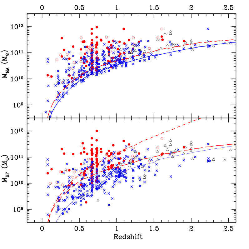
Figure 1: Galaxy stellar masses in the K20 sample as a function of redshift. Upper panel: estimates based on Maximal Age model. Lower panel: estimates based on the Best Fit method. Filled circles: early type galaxies; empty circles: early$+$emission type; crosses: “star–forming” type; triangles: objects with photometric redshifts. A few very low redshift objects at $M_{*}<7\times 10^{8}M_{\odot}$ are omitted. The short and long dashed lines correspond to the completeness threshold, define by computing a maximally massive model with $K_{s}=20$, considering dust and dust-free models, respectively (see text for details). Solid lines correspond to the selection curves that we have applied when building the Galaxy Stellar Mass Function, after application of the appropriate correction for incompleteness as described in Sect. 5 and Appendix B.

The derived masses for the K20 sample are shown in Fig. 1 as a function of redshift. For each object, both the MA (upper panel) and the BF estimates (lower panel) are shown. It is immediately apparent that very massive galaxies, in the range $10^{11}M_{\odot}<M_{*}<10^{12}M_{\odot}$, are detected all the way to $z\simeq 2$. Besides the $M_{*}\simeq 10^{12}M_{\odot}$ galaxies within the two $z\simeq 0.7$ peaks, the most massive galaxy with spectroscopic redshift in the K20 sample is CDF1-633 at $z_{\rm spe}=1.096$, $M_{*}=(4-8)\times 10^{11}M_{\odot}$, according to the BF and the MA method, respectively.

In the HDFN, the upper envelope of the mass distribution appears to decrease at high redshift (D03). Such a trend is much less clear in the similar analysis of the HDFS (F03), and even less so in the present K20 sample.

Conversely, the lower envelope is a result of the $K<20$ selection criteria, that prevents less massive objects to be detected. However, as already discussed by D03 and F03, IR–selected samples do not strictly correspond to mass–selected ones. Indeed, at any Hubble time (i.e. redshift), for each $K$-band luminosity there is a range in the possible $M_{*}/L$ ratios that is set by the range of allowable ages, metallicities and dust extinctions of the observed stellar population. This implies that at the low mass side the sample is progressively biased against the detection of high $M_{*}/L$ , such as old, passively evolving or highly extincted galaxies.

Because of the uncertainties in the modeling of such objects, it is difficult to define a clear mass threshold as a function of redshift. A very conservative way to estimate it corresponds to the minimum mass that a $K_{s}=20$ galaxy at any given redshift may have, within the adopted set of spectral templates. Such a threshold strongly depends on the adopted library, and in particular on the allowed maximum extinction. For both BF library, this threshold is shown as short dashed lines in Fig. 1. In this case, this threshold corresponds to the maximum extinction allowed in the set of templates (which is entirely arbitrary) and it would eliminate a large fraction of the sample from the statistical analysis. A more realistic approach (already adopted by D03 and F03) is to consider only dust-free, passively evolving models, such that the derived threshold corresponds to the selection for early type galaxies. In the case of both the MA and BF libraries, this is shown as a long dashed line in Fig. 1. Our sample is therefore definitely incomplete below this curve, where several objects of lower $M_{*}/L$  (typically star–forming galaxies) are still detected, and reasonably complete above, except for strongly obscured sources. The selection curves in Fig. 1. shows that our sample is “mass–complete”, except for strongly obscured sources, down to objects of $M_{*}\simeq 3\times 10^{10}M_{\odot}$ at $z\simeq 1$, and of $M_{*}\simeq 2\times 10^{11}M_{\odot}$ up $z\simeq 2$.

In principle, only objects above the long dashed lines of Fig. 1 should be used in statistical analyses that require mass–selected samples, such as average $M_{*}/L$ , mass densities or mass functions. In the Section 5.1 and in Appendix B we will describe how we have introduced a correction for the incompleteness in order to extend the construction of the mass function to lower masses. Thanks to this approach, we will be able to recover a significant fraction of our sample: the corresponding selection curves are shown as solid lines in Fig. 1.

4.2 The $M_{*}/L$ ratio

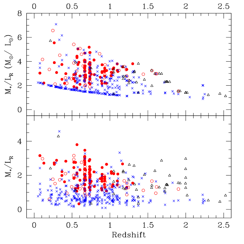
Figure 2: $M_{*}/L_{R}$ ratios as a function of redshift, in the K20 sample. Upper panel shows the Maximal Age estimates, while lower one shows the Best Fit ones. In both panels the symbols correspond to different spectral types, as in Fig. 1.

Fig. 2 shows the values of the $M_{*}/L_{R}$ ratio for the K20 sample of galaxies as a function of redshift, as derived from the MA and BF procedures. Here, $L_{R}$ is the absolute luminosity in the rest-frame $R$ band, in solar units, which is extracted from the spectral template that best-fits the corresponding observables, and that is well sampled by our multicolor photometry up to $z\simeq 2$. For the reasons described above, the $M_{*}/L_{R}$ ratio tends to be higher in the MA models than in the BF ones. Using the “mass complete” sample described in Appendix B, we have obtained the average $M_{*}/L_{R}$ ratio for the whole sample and for the two spectral types as a function of redshift (in the redshift bins adopted to compute the galaxy stellar mass function). The corresponding values are shown in Table 2, along with the corresponding dispersions in the data.

In the redshift range including most of the galaxies in the sample ($0.2\leq z\leq 1.5$), a correlation exists between the average $M_{*}/L_{R}$  ratio and the observed spectral type, with the spectroscopic early type galaxies having on average a higher $M_{*}/L_{R}$  ratio with respect to the late type, star-forming ones. In addition, we also detect an overall trend of decreasing $M_{*}/L_{R}$  with increasing redshift, for both the early and the late type galaxies.

It is of some interest to compare the observed $M_{*}/L_{R}$  ratio of early type galaxies with that expected in simple cases of PLE models. We plot in Fig. 3 the $M_{*}/L_{R}$  for spectroscopically early and early$+$emission types as a function of redshift, differentiating between brighter ($M_{R}<-22$) and fainter ($M_{R}\geq-22$) objects, and compare the observed evolution with a set of single-exponential models with $z_{\rm form}=3$ and $20$ and $\tau=0.1$ and $3$ Gyrs, all computed with a Salpeter IMF and no dust extinction. For simplicity, we plot only the BF estimates. It is shown that the observed $M_{*}/L_{R}$  values are distributed over a significant range, suggesting that coeval, single–exponential models are probably an oversimplified way to describe the properties of spectroscopically early type galaxies. A similar result was also presented on the EROs subsample (Cimatti et al 2003), and is now extended to the whole early type population.

More interestingly, we show that the typical $M_{*}/L_{R}$  of brighter objects is significantly larger than that of the fainter ones at low and intermediate redshifts. This implies that, while the $M_{*}/L_{R}$  of the bright population is consistent with either very short star–formation time-scales or high $z_{form}\geq 3$, and some objects appear to require both, the fainter population has experienced a more recent history of assembly, witnessed by the larger $\tau$ and lower $z_{form}$ required to reproduce the typical $M_{*}/L_{R}$ . So, the most luminous and massive galaxies appear to reach near completion first, while less massive ones keep growing in mass till later times. This down-sizing effect was first noted by Cowie et al. (1996) for $z\lower 2.15277pt\hbox{$\;\buildrel>\over{\sim}\;$}1$, and then explicitly quantified by Brinchmann and Ellis 2000 and F03 (see also Kodama et al. 2004). This tendency continues all the way to $z\sim 0$, where the star-formation rate per unit mass anti-correlates with galaxy mass (Gavazzi et al. 1996; Kauffman et al. 2003).

Table 2: Average $M_{*}/L_{R}$ ratios as a function of redshift and spectral type, computed in the mass complete–sample, as defined by the thick solid curve of Fig. 1. All refers to all galaxies in the K20 sample, including also those with photometric redshift only. Early refer to early and early+emission spectroscopic types and late to late spectroscopic types, as defined in Section 2. Only objects with spectroscopic redshift are included in the last two columns. $M_{*}/L$   ratio in the V and K bands are available in electronic form at the web site http://www.arcetri.astro.it/^∼k20

$$\begin{array}[]{|l|ccc|ccc|ccc|}\hline\cr\nobreak\leavevmode&\lx@intercol\hfil\rm MaximalAge\hfil\lx@intercol\vrule\lx@intercol\\ \hline\cr{\rm Redshift}&\lx@intercol\hfil\rm All\hfil\lx@intercol\vrule\lx@intercol&\lx@intercol\hfil\rm Early\hfil\lx@intercol\vrule\lx@intercol&\lx@intercol\hfil\rm Late\hfil\lx@intercol\vrule\lx@intercol\\ \hline\cr\nobreak\leavevmode&\it n&\frac{M}{L_{R}}&\sigma&\it n&\frac{M}{L_{R}}&\sigma&\it n&\frac{M}{L_{R}}&\sigma\\ z<0.2&\it 9&2.83&0.82&\it 3&3.13&0.98&\it 6&2.67&0.78\\ 0.2\leq z\leq 0.7&\it 148&3.02&1.30&\it 69&3.46&0.90&\it 76&2.49&1.22\\ 0.7\leq z\leq 1.0&\it 89&2.93&0.91&\it 45&3.31&0.73&\it 44&2.54&0.93\\ 1.0<z\leq 1.5&\it 71&2.65&0.75&\it 18&3.19&0.38&\it 43&2.34&0.76\\ 1.5<z\leq 2.0&\it 19&2.39&0.66&\it 5&2.74&0.69&\it 3&1.73&0.45\\ \hline\cr\nobreak\leavevmode&\lx@intercol\hfil\rm BestFit\hfil\lx@intercol\vrule\lx@intercol\\ \hline\cr{\rm Redshift}&\lx@intercol\hfil\rm All\hfil\lx@intercol\vrule\lx@intercol&\lx@intercol\hfil\rm Early\hfil\lx@intercol\vrule\lx@intercol&\lx@intercol\hfil\rm Late\hfil\lx@intercol\vrule\lx@intercol\\ \hline\cr\nobreak\leavevmode&\it n&\frac{M}{L_{R}}&\sigma&\it n&\frac{M}{L_{R}}&\sigma&\it n&\frac{M}{L_{R}}&\sigma\\ z<0.2&\it 10&1.77&0.94&\it 3&2.95&0.22&\it 7&1.27&0.56\\ 0.2\leq z\leq 0.7&\it 104&1.92&0.83&\it 61&2.18&0.66&\it 42&1.48&0.82\\ 0.7\leq z\leq 1.0&\it 65&1.73&0.49&\it 47&1.86&0.45&\it 18&1.40&0.45\\ 1.0<z\leq 1.5&\it 38&1.78&0.54&\it 16&1.61&0.45&\it 16&1.81&0.62\\ 1.5<z\leq 2.0&\it 15&1.53&0.53&\it 5&1.35&0.30&\it 2&1.26&0.43\\ \hline\cr\hline\cr\end{array}$$

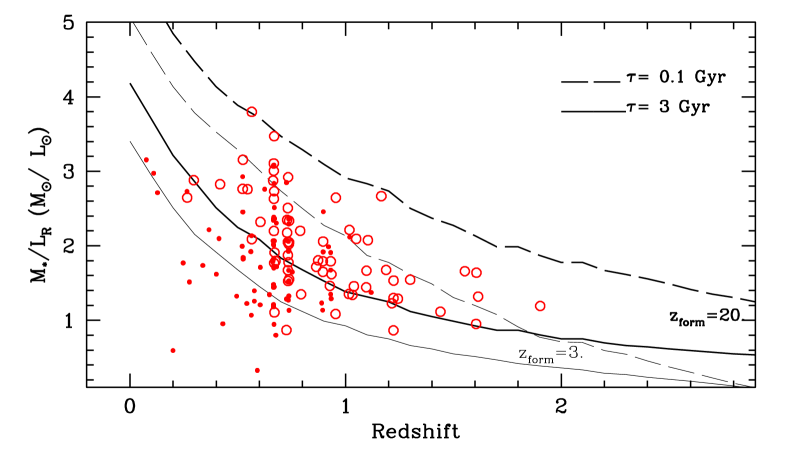
Figure 3: $M_{*}/L_{R}$ ratios as a function of redshift for spectroscopically early and early$+$emission spectral type galaxies of the K20 sample. Large hollow circles are for bright ($M_{R}<-22$) objects, small filled circles for fainter ($M_{R}>-22$) ones. Lines show the $M_{*}/L_{R}$  values computed with a set of single–exponential models with $z_{\rm form}=3$ (thin lines) or $z_{\rm form}=20$ (thick lines) and star–formation time-scales ranging of $\tau=0.1$ Gyr (dashed lines) and $\tau=3$ Gyr (solid lines), all drawn with a Salpeter IMF and no dust extinction.

5 Galaxy Stellar Mass Functions

5.1 The construction of the Galaxy Stellar Mass Functions

Once the stellar mass has been obtained for each galaxy in the sample, the building of the corresponding Galaxy Stellar Mass Function (GSMF) follows the traditional techniques used for luminosity functions. We apply here both the classical $1/V_{\rm max}$ formalism to obtain binned distributions, and the Maximum Likelihood technique to estimate the best-fit Schechter parameters, using the recipes described in Poli et al. (2001, 2003) and Pozzetti et al. (2003), and references therein.

With respect to the standard procedures adopted for luminosity functions, an improvement is necessary to account for the incompleteness in the mass census of galaxies. The adopted procedure to obtain the correction fractions for incompleteness is fully described in Appendix B. This correction factor is then applied to the volume element $V_{\rm max}$ of any galaxy, both in the $1/V_{\rm max}$ binned GSMF as well as in the Schechter best-fits.

Another aspect requiring particular attention is the comparison of GSMFs derived at the various redshifts with the local, $z\sim 0$ GSMF. In the following, we shall make use of the local GSMFs derived by Cole et al. (2001) and Bell et al. (2004) with the same Salpeter IMF. The former authors estimate the spectral type by the observed $J-K$ color, while the latter ones use the complete set of $ugrizJHK$ SDSS+2MASS colors. Since both authors use a set of spectral synthesis models with star-formation rate peaking at high redshifts, the two GSMFs agree quite well with each other, especially for $M_{*}>10^{10}M_{\odot}$, and the comparison with our MA estimates at higher redshift is fair, since our MA method mimics exactly the Cole et al. (2001) models.

Conversely, the same may not hold for our BF estimates, that have no constraint on age and typically yield lower $z_{\rm form}$ for the K20 objects. To estimate the effect, we have repeated the Bell et al. (2004) procedure, building a sample of 6332 SDSS+2MASS local galaxies, for which we obtained both the MA and BF stellar masses with our recipes. For this local sample we find that the BF mass estimates are on average lower than MA by only about 20%, and even less for more massive objects. Full details of this analysis are described in Appendix A.5. Using this result to statistically convert the Cole et al. (2001) mass function to a BF one, we have obtained a “BF–scaled” local GSMF that only marginally departs from the original of Cole et al. (2001) in the massive tail, and that we will use to compare with our “BF” results at higher $z$.

Finally, the intrinsic uncertainty in the estimate of the stellar mass must be taken into account when computing the error budget in the GSMF. At this purpose, we have performed a set of MonteCarlo simulations where the input mass catalogs were randomly perturbed, allowing each galaxy in the sample to move around its best fit values of a quantity specified (for each galaxy) by the error analysis described in Appendix A.4. This includes also the uncertainty due to the redshift for galaxies with photometric redshifts only. We simulated 200 such catalogs, and computed the resulting GSMF. The dispersion in the derived values (both for the binned valued as well as for the fitted Schechter parameters) has been added in quadrature to the standard Poisson noise for each GSMF. We remark that a more global uncertainty - not shown in the following figures - is related to cosmic variance, that is much more difficult to treat. As we discuss in better detail in Sect. 5.5, the error budget due to cosmic variance is around 20-40% (depending on the assumed galaxy correlation length) of the total number densities.

5.2 The evolution of the Galaxy Stellar Mass Functions

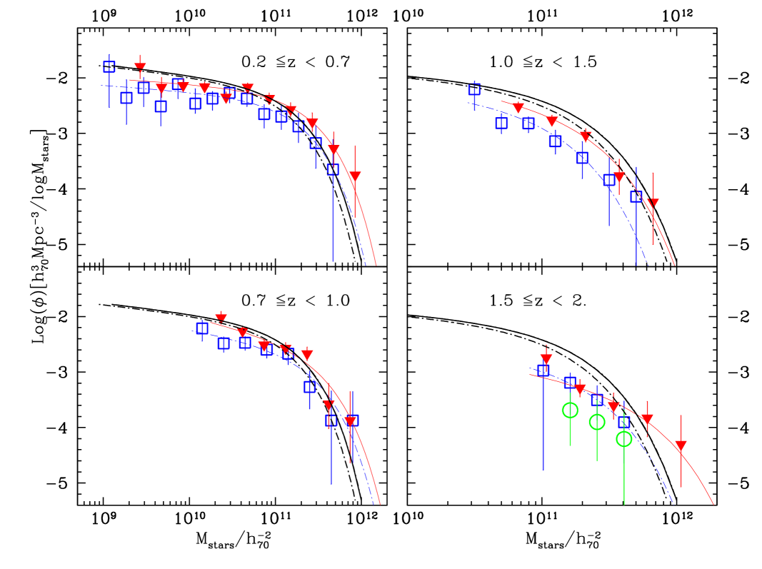
Figure 4: Galaxy stellar mass functions in the K20 sample, in four redshift ranges. Different symbols correspond to different methods adopted to estimate the stellar mass: triangles represent the Maximal Age estimates, and squares the Best Fit estimates. In the highest redshift bin, large hollow circles correspond to the GSMF measured by using only objects with spectroscopic redshift. Thick lines correspond to local galaxy mass functions: the solid line is the local galaxy mass function by Cole et al. (2001), the dot–dashed one is the same GSMF renormalized to our “BF” method (See text and appendix A for details). The same line types have been used to represent the Schechter fits to our “extended” galaxy mass functions (thin lines).

The resulting stellar mass functions of the K20 sample are shown in Fig. 4. We have divided the sample into four redshift bins: 0.2–0.7; 0.7–1.0; 1.0–1.5; and 1.5–2.0, having chosen the two lowest redshift bins in such a way to distribute in two different bins the impact of the two redshift peaks at $z=0.67$ and $z=0.73$, and to have a similar comoving volume (about $2.5\times 10^{4}$Mpc³). The two high redshift bins have also a comparable comoving volume ($7\times 10^{4}$Mpc³ and $8.2\times 10^{4}$Mpc³, respectively). We have restricted the estimate of the GSMF at $z<2$, given the small number of objects and the limited mass range covered by our sample beyond $z\simeq 2$. The average redshift of the galaxies in each bin is $0.52,0.83,1.17$ and $1.72$, respectively. In terms of cosmic time, for the adopted cosmology these redshift intervals correspond to an age of the Universe of $11.3-7.5$, $7.5-6.1$, $6.1-4.6$ and $4.6-3.6$, respectively. For each redshift bin we have constructed the GSMF following the two different methods described in the previous sections: Maximal Age and Best Fit. For each bin, error bars include both the Poisson noise (computed using the exact formulas for low counts given in Gehrels (1986)) as well as the uncertainty in mass estimates, obtained with the Monte Carlo procedure described above.

In the highest $z$ bin, the contribution by objects which have only a photometric redshift is significant. In order to provide a strict lower limit to the total GSMF, in this redshift bin we have also used only the spectroscopic sample with no correction for incompleteness (large hollow circles in Fig. 4).

Table 3: Best fit Schechter parameters of the Galaxy Stellar Mass Functions in the K20 survey. Errors indicate $1\sigma$ confidence levels. Parameters without error have been fixed to the best fit value of the lower $z$ bin.

$$\begin{array}[]{|l|l|ccc|}\hline\cr\vrule\lx@intercol\hfil\rm Schechter\leavevmode\nobreak\ Parameters\leavevmode\nobreak\ for\leavevmode\nobreak\ the\leavevmode\nobreak\ GSMF\hfil\lx@intercol\vrule\lx@intercol\\ \hline\cr{\rm Redshift}&\nobreak\leavevmode&\alpha&M^{*}&\phi^{*}\\ \hline\cr 0.2\leq z<0.7&{\it BF}&-1.11\pm 0.10&11.22^{+0.13}_{-0.12}&0.00182\\ 0.2\leq z<0.7&{\it MA}&-1.10\pm 0.10&11.32\pm 0.11&0.00252\\ \hline\cr 0.7\leq z<1.0&{\it BF}&-1.27\pm 0.23&11.37^{+0.22}_{-0.21}&0.00110\\ 0.7\leq z<1.0&{\it MA}&-1.36\pm 0.23&11.44\pm 0.19&0.00132\\ \hline\cr 1.0\leq z<1.5&{\it BF}&-1.27&10.99^{+0.16}_{-0.1}&0.00147\\ 1.0\leq z<1.5&{\it MA}&-1.36&11.20\pm 0.08&0.00150\\ \hline\cr 1.5\leq z<2.&{\it BF}&-1.27&11.24^{+0.38}_{-0.18}&0.00067\\ 1.5\leq z<2.&{\it MA}&-1.36&11.63\pm 0.17&0.00026\\ \hline\cr\hline\cr\end{array}$$

At each redshift, the resulting GSMFs are compared to the local one by Cole et al. (2001) for the same Salpeter IMF, as well as to the one “rescaled” to our BF estimates (see appendix A5, Fig. 15). For simplicity, we do not plot the Bell et al. (2004) local GSMF, that is in excellent agreement with Cole et al. (2001) mass function.

In each panel of Fig. 4 we also plot the Schechter fits of the “extended” GSMFs. We remark that the Schechter parameters derived by using the “strictly complete” or the “extended” selection criteria are statistically consistent with each other. Unfortunately, at $z>1$, we cannot reliably estimate the slope of the GSMF because of the small range in mass covered by our sample. For this reason, we have assumed in these bins the same slope that we observe at $0.7\leq z<1$, which may bias the estimate of the characteristic mass in the high $z$ bins. For this reason, and given the size of the resulting statistical errors, one should not read too much in these values, that should be primarily used as description of our dataset in the range that we actually observe. The corresponding best fit values are given in Table 3, with their $1\sigma$ uncertainties.

The most relevant results that emerge from Fig. 4 are the following:

First, we note that the overall agreement between the GSMF derived with the BF and the MA procedures is fairly satisfactory. Albeit MA estimates provide higher normalizations than the BF estimates, as expected by their typically larger masses, the resulting scenarios are not significantly dependent on the adopted method of mass determination, and so are the conclusions that we shall draw in the following.

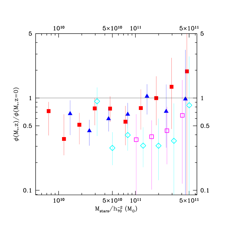
Figure 5: Ratio between the observed Galaxy Stellar Mass Functions in the K20 sample and the local GSMF. Data points refer to the ratio of the “Best Fit” values to the corresponding “rescaled” local GSMF. Filled symbols refer to points at $z<1.0$ (squares: $0.2<z<0.7$; triangles $0.7<z<1.0$); open symbols to $z>1.0$ (diamonds: $1.0<z<1.5$, squares: $1.5<z<2$). The data points at $1.5<z<2$ include objects with photometric redshifts.

Up to $z\simeq 1$ there appears to be only a very mild evolution of the GSMF (see Fig. 4 and Fig. 5), as suggested by the corresponding near-IR luminosity function (Pozzetti et al. 2003). Both the MA- and the BF-derived GSMFs are in agreement with the local ones, at least in the range $10^{10}M_{\odot}<M_{*}<2\times 10^{11}M_{\odot}$, where our statistics is reasonably accurate. The low-mass end of the GSMF is rather flat in the first redshift bin, where it is well determined ($\alpha=-1.1\pm 0.1$), quite consistent with the local estimates ($\alpha=-1.18\pm 0.03$) (Cole et al. 2001); in addition, also the characteristic masses in the Schechter function are consistent with local estimates.

At higher redshifts, $z>1$, there appears to begin a decrease in the normalization of the GSMF, which is particularly remarkable if we take into account the relatively small range of cosmic time resulting from our sampling. The decrease is particularly evident for $M_{*}\simeq 10^{11}M_{\odot}$, and is approximately constant up to $z\simeq 2$. This decrease in normalization is also shown in Fig. 5, where we plot the ratio between the GSMF at the various redshifts and the local GSMF for the BF case. The number density of objects around $M_{*}\simeq 10^{11}M_{\odot}$ is (70-80%) of the local value up to $z\simeq 1$, while it decreases to (30-40%) of the local value in the two higher redshift bins. This suggests that the mass assembly of objects with mass close to the local characteristic mass was quite significant between $z=2$ and $z=1$, and was essentially complete by $z\simeq 1$.

The evidence presented in Sect. 4.2 of a differential evolution of early type galaxies, with more luminous (i.e. more massive) galaxies having formed earlier than less luminous one, should be reflected in a flattening of the observed GSMF at high $z$. In our data there is a tentative suggestion of this, since the massive tail of the GSMF appear to evolve in a slower fashion than the fainter. Given the present statistics, unfortunately, much wider surveys are required to confirm this potentially important item.

5.3 The GSMF for different spectral types

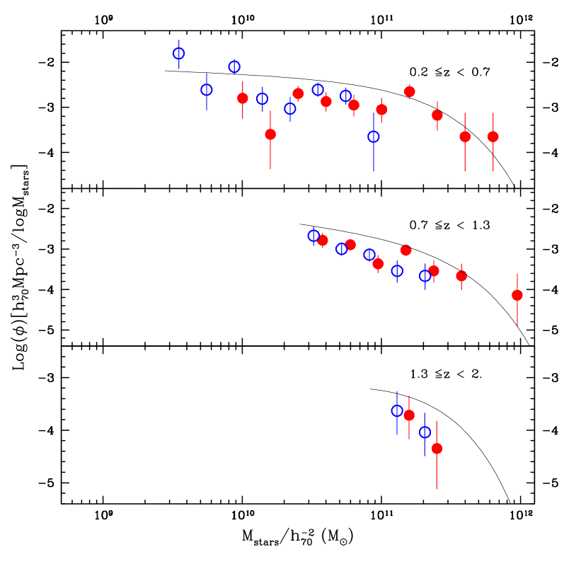
Figure 6: Galaxy stellar mass functions in the K20 sample for different spectral types. Empty points correspond to late spectral type, filled to early spectral type. The solid lines show the Schechter fits to the total GSMF of our sample at the corresponding redshifts.

Fig. 6 shows the GSMF for the two main broad galaxy spectral types, early and late (we remark that early$+$emission type have been omitted). Since only objects with spectroscopic redshift are included, these were grouped into three bins rather than four as in Fig. 4, thus ensuring a fairly good statistics in each bin. We remind that the spectroscopic completeness of the K20 survey is particularly high ($\simeq 92\%$), such that incompleteness effects should play a minor role here. In any case, one expects galaxies without a spectroscopic redshift to be preferentially at $z\lower 2.15277pt\hbox{$\;\buildrel>\over{\sim}\;$}1.3$, for which the most prominent spectral features have moved out of the observed spectral range. For $z<1.3$, indeed, we estimate the spectroscopic completeness to be 97%, given the distribution of the photometric redshifts of the unidentified objects.

We find that there is a clear difference in the GSMF for the two spectral types (Fig. 6). Up to $z\simeq 1.3$, early type galaxies dominate the mass distribution, and in practice provide the whole contribution to its most massive side. This can be qualitatively appreciated by observing the GSMF of Fig. 6 and by observing that all the more massive galaxies at these redshift bins are early type. Although the latter evidence may be somewhat affected by the prominent structures at $z\simeq 0.7$, that are dominated by early type galaxies, a scrutiny of our catalogs reveals that early type galaxies are the most massive galaxies also outside the structures (see Fig. 1). Quantitatively, we find indeed that the stellar mass density due to massive galaxies (i.e. $M_{*}\geq 10^{11}M_{\odot}$) at $z\simeq 0.45$ and $z\simeq 1$ is of 1.68 and 1.08 $10^{8}M_{*}$Mpc^-3, of which 85% and 69%, respectively, is due to early type galaxies, and 0% and 16% is due to late type galaxies. When integrated over the whole observed range early type galaxies provide about 60% of the whole stellar mass density at $z<1.3$. A similar behavior was found in the local GSMF by Bell et al. (2004), where the early-type/late-type classification was based on morphology.

In the highest redshift bin, star–forming galaxies appear to contribute a significant fraction of the massive tail of the GSMF. The measured stellar mass density at $1.3<z<2$ due to star-forming galaxies with $M_{*}\geq 10^{11}M_{\odot}$ is of the order of $1\times 10^{7}M_{\odot}/$Mpc^-3, corresponding to about 21% of the total mass density in the same mass range, an amount nearly identical to the contribution of early type galaxies (22%). This figure is a lower limit to the contribution of late-type galaxies to the total stellar mass density, since it would correspond to assuming that all the galaxies without spectroscopy in this redshift bin are passively evolving objects (which implies that all photometric redshifts are correct in this range and that all unidentified objects are spectroscopically early type).

Irrespective of the nature of the unidentified objects, this result suggests that a global physical change occurs at larger and larger $z$, with an increasing fraction of the stellar mass density being contained in actively star–forming objects. This is also supported by the upper limit to the global stellar mass density in passively evolving galaxies at $z\simeq 3$, that is about 40% of the total (at $z=\simeq 3$) in the HDFS (F03).

5.4 The cosmological evolution of the mass density

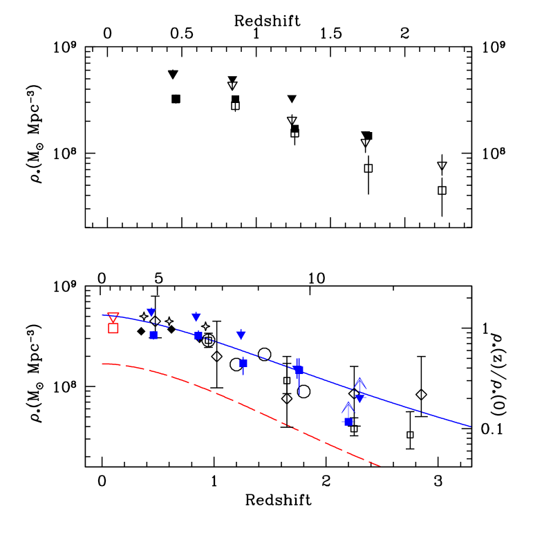
Figure 7: Evolution of the cosmological mass density as a function of redshift. Upper panel: Observed cosmological mass density as observed in the K20 data. Squares correspond to BF estimates, Triangles to MA estimates. Empty points represent the observed values, with the corresponding Poisson noise. Filled points represent the values corrected for incompleteness, as obtained by integrating the mass function over the whole range $10^{8}M_{\odot}\leq M_{*}\leq 10^{13}M_{\odot}$. Error bar are computed from the uncertainties in the best–fit parameters of the Schechter Function. Lower panel: The global evolution of the cosmological mass density from $z=0$ to $z=3$ as observed from the K20 and other surveys. Filled points represent the total values from the K20 survey: squares are the “Best Fit” values and triangles the “Maximal Age” estimates. The points at $<z>=2.25$ are lower limit since they are affected by incompleteness. The large open triangle is the local value by Cole et al. 2001, while the large open square is the same local value rescaled to the BF technique. Open exagones are from Cohen et al. 2001, open triangles from Brinchmann and Ellis 2000, open squares from D03, diamonds from F03, empty circles from Glazebrook et al. 2004. Error bars in the latter two surveys take into account for the systematic uncertainties among the methods adopted, as in the case of our MA and BF approaches. The two lines are the mass densities expected by integrating the star formation histories of Steidel et al. 1999 for two different extinction coefficients (dashed: $E(B-V)=0$; solid: $E(B-V)=0.15)$.

The upper panel of Fig. 7 shows the stellar mass density $\rho_{*}(z)$, as derived for the K20 sample with the two different methods (BF and MA), both from the observed data, as well as from the incompleteness-corrected GSMFs, i.e., integrating the best–fit Schechter functions (Table 3) over the whole range $10^{8}M_{\odot}\leq M_{*}\leq 10^{13}M_{\odot}$. The same quantites are given in Tab.4. The correction is marginal at $z<1$, but becomes a factor of $\sim 2$ at $z\geq 1.5$, where this exercise is obviously prone to statistical as well as systematic errors due to the limited mass range of the observed GSMF. Fig. 7 gives the statistical errors due to the uncertainties in the best-fit parameters of the Schechter function.

In the case of the two high redshift bins, where we have fixed the slope of the GSMF (see Tab.3), these error estimates do not take into account the uncertainty in the slope of the GSMF: this systematic effect is discussed and quantified in Sect. 5.5, as well as the global uncertainty due to cosmic variance.

The global evolution of the stellar mass density from the K20 sample is reported again in the lower panel of Fig. 7, along with the results from other surveys at $z\simeq 1$ (Brinchmann and Ellis 2000; Cohen 2002), as well as at higher $z$ from Glazebrook et al. 2004 and from the HDFN (D03) and HDFS (F03). The K20 survey data show that the stellar mass density at $z\simeq 1.5-2$ is about 35% of the local value, with a lower limit (given by the strictly observed quantity) of 20%. This is well placed within the global trend that witnesses a fast increase of the stellar mass density from $20^{+20}_{-10}\%$ of the local value at $2<z<3$ to about unity at $z\leq 1$, i.e. in a relatively short span of cosmic time. At $z>2$, we cannot compute a reliable estimate of the total mass density since most of the objects fall below the completeness threshold. For this reason, we compute the same quantity on the observed data only, and represent it as a lower limit. Interestingly, this quantity seems to support the higher values observed in the HDFS rather than those in the HDFN.

While the current, direct estimate is still affected by sizable uncertainties, it is worth considering the indirect estimate of the fraction of the stellar mass already in place at high redshift which is provided by the low redshift “fossil” evidence. Indeed, from the fraction of the local stellar mass locked in passively evolving spheroids ($\sim 50-75\%$; e.g., Persic & Salucci 1992; Fukugita et al. 1998; Benson et al. 2002), and from the high redshift of formation ($z\lower 2.15277pt\hbox{$\;\buildrel>\over{\sim}\;$}3$) for the bulk of stars in such spheroids (Renzini 1999a), it has been inferred that at least $\sim 30\%$ of the local stellar mass may well be already in place by $z=3$ (Renzini 1998, 2003).

Table 4: Observed and total stellar mass density in the K20 survey, as a function of redshift. Reference value are given for the BF estimates; lower errors take into account the Poisson noise and the uncertainties in the mass estimates. Upper limits have been computed with respect to the values provided by the MA method, to provide an estimate of the global uncertainties.

$$\begin{array}[]{|l|ccc|}\hline\cr\vrule\lx@intercol\hfil\rm Stellar\leavevmode\nobreak\ Mass\leavevmode\nobreak\ Density\leavevmode\nobreak\ in\leavevmode\nobreak\ the\leavevmode\nobreak\ K20\leavevmode\nobreak\ survey\hfil\lx@intercol\vrule\lx@intercol\\ \hline\cr\hline\cr{\rm Redshift}&{\rm Observed^{\mathrm{a}}}&{\rm Total^{\mathrm{b}}}&M_{*}\simeq 10^{11}M_{\odot}^{\mathrm{c}}\\ \hline\cr\nobreak\leavevmode&log(M_{*}/M_{\odot})&log(M_{*}/M_{\odot})&log(M_{*}/M_{\odot})\\ \hline\cr 0.2\leq z<0.7&8.51^{+0.24}_{-0.04}&8.51^{+0.26}_{-0.04}&8.32^{+0.28}_{-0.04}\\ \hline\cr 0.7\leq z<1.0&8.44^{+0.20}_{-0.05}&8.50^{0.23}_{-0.05}&8.29^{+0.20}_{-0.04}\\ \hline\cr 1.0\leq z<1.5&8.19^{+0.13}_{-0.11}&8.23^{+0.33}_{-0.11}&7.88^{+0.39}_{-0.1}\\ \hline\cr 1.5\leq z<2.&7.86^{+.24}_{-.24}&8.16^{+0.11}_{-0.24}&7.93^{+0.1}_{-0.22}\\ \hline\cr 2\leq z<2.5^{\mathrm{d}}&7.65^{+.24}_{-.24}&-&-\\ \hline\cr\end{array}$$

• On the complete sample

• Computed extending the Schechter fits from $10^{8}M_{\odot}$ to $10M_{\odot}$.

• Computed for objects with $5\times 10^{10}M_{\odot}\leq M_{*}\leq 5\times 10^{11}M_{\odot}$.

• This value is actually a lower limit: see text for detail.

Following the approach of Pozzetti et al. 1998, D03 and Cole et al. (2001), the lower panel of Fig. 7 shows a comparison of $\rho_{*}(z)$ from various surveys with the same quantity as obtained by integrating over time the star-formation rate density from Steidel et al. (1999), with two different assumptions for the dust extinctions (i.e., $E(B-V)=0.0$ and 0.15). There appears to be a good agreement between the observed evolution of $\rho_{*}(z)$ and the integrated star–formation history due only to UV bright galaxies, after allowing for a reasonable amount of dust.

Given the uncertainties in the estimates of both the stellar masses and the UV–corrected star–formation rates, it is still possible to allocate space for other significant contributors to the global star–formation rate, as could be the case of dust–enshrouded sources. However, the overall agreement, and in particular the match with the local value of the stellar mass density, as well as the consistency with the luminosity densities at different wavelengths up to $z\simeq 1$ (Madau, Pozzetti and Dickinson 1998), appear to support the notion that the UV selection is able to recover a major fraction of the star-formation activity at high redshift.

5.5 Systematic uncertainties

In closing this section it is worth emphasizing that several systematic uncertainties still affect the mass estimates of individual galaxies as well as the current estimates of the global mass density at high redshift. Such uncertainties are cursorily listed below.

$\bullet$ Initial Mass Function. The Salpeter IMF ($\phi(M)\propto M^{-2.35}$ from 0.1 to 100 $M_{\odot}$) was adopted to allow a direct comparison with other observational or theoretical GSMFs. However, all empirical determinations of the IMF indicate that its slope flattens to $\sim-1.35$ below $\sim 0.5\;M_{\odot}$ (Kroupa 2001), including data both in the Galactic disk (Gould et al. 1996) and in the Galactic bulge (Zoccali et al. 2000). Compared to the single-slope Salpeter IMF, such a two-slope IMF would give masses about a factor of 2 smaller, for a given galaxy luminosity. However, this correction applies by about the same factor at all redshifts explored in this paper, and the relative evolution of the GSMF is not affected. Of more concern is the possibility of a different slope for $M\lower 2.15277pt\hbox{$\;\buildrel>\over{\sim}\;$}M_{\odot}$. The use of a top-heavy IMF would appreciably reduce the estimated masses of actively star-forming galaxies at high redshifts, and would appreciably modify the evolution of the GSMF derived from the present data. On the other hand, a top-heavy IMF would largely over produce metals compared to their observed amount in galaxy clusters (Renzini 1999b), while probably leading to a too small star mass density in the local universe. Nevertheless, a more systematic exploration of other assumptions on the IMF may have been in order, but this goes beyond the scope of the present paper.

$\bullet$ Spectral coverage. As the redshift increases, a bluer and bluer portion of the rest-frame spectrum is used, which is progressively dominated by the young-age, low-mass components of galaxies, rather than by the older, more massive components. This might lead to an underestimate of the stellar mass at high redshift. A quantitative estimate of this effect should soon become possible as the Spitzer observatory will directly provide rest-frame $K$-band luminosities all the way to $z\sim 3$ for galaxies in the GOODS fields (Dickinson 2002).

$\bullet$ Highly obscured objects. A $K$-band selection of galaxies to trace the build-up of stellar mass is certainly the least biased approach to the problem, yet one not totally free from a selection bias. Highly obscured objects at high $z$, such as SCUBA sources (Chapman et al. 2003), may well be fainter than our threshold at $K_{s}=20$ and nonetheless they may contain a sizable fraction of the stellar mass in the highest redshift bin, while experiencing extreme starbursts. Again, this bias would introduce an underestimate of the total stellar mass at high redshift.

$\bullet$ Shape of the Mass Function. The incomplete coverage of the mass function increases with redshift, hence the uncertainty in the slope $\alpha$ of the GSMF increases with redshift (see Table 3), such that we have been forced to fix the slope at $z>1$. In the case that the high $z$ GSMF is steeper than our assumption, this would lead to an underestimate of the stellar mass density in the two high $z$ bins, and to a (slight) overestimate in the opposite case. For instance, the total mass density that we estimate in the redshift range $z=1.0-1.5$ would result $\rho=10^{8.21}$,$10^{8.34}$,$10^{8.52}$ if the slope of GSMF is fixed to $\alpha=-1.18,-1.5,-1.8$, respectively. Only substantially deeper data could improve the present estimates of the GSMF.

$\bullet$ Cosmic variance. While some 10 times larger than HDF, the area explored by the K20 survey is still quite small, likely to be subject to sizable fluctuations in the number density of highly-clustered massive galaxies. For example, field-to-field variance is detected among COMBO-17 fields (Bell et al. 2004), each of them almost 20 times the area covered by the K20 project. Indeed, as mentioned in Section 2, the K20 sample exhibits redshift peaks that appear to be significantly above the average distribution at $z\leq 1$, and strong clustering among early type red galaxies (EROs) is detected in our sample at $z\simeq 1$ (Daddi et al. 2002).

For the reasons described in Section 2, however, the number of these structures is reasonably within the expectation, such that we do not have any reason to remove them nor any statistical argument to re-normalize their contribution.

Even in this case, the cosmic variance due to galaxy clustering may affect our results. To estimate this effect, we have assumed two possible values for the galaxy correlation lenghts, $r_{0}=5h^{-1}$Mpc and $r_{0}=10h^{-1}$Mpc, respectively, and computed the expected variance using Eq. 8 of Daddi et al. 2000. The value $r_{0}=5h^{-1}$Mpc has been derived from an analysis of the clustering observed in the K20 sample itself, of which we shall provide the details elsewhere, while $r_{0}=10h^{-1}$Mpc is a safe upper limit taken from the EROs clustering amplitude (Daddi et al. 2001). We find that the relative variances in our redshift bins are typically of about 20-25% in the former case, and 40% in the latter. If we restrict the computation to massive objects ($M_{*}\geq 10^{11}M_{\odot}$), which dominate the mass density, the expected variance are only slightly larger, 30% and 45% respectively.

Ultimately, surveys over much wider areas will be necessary to fully average out the impact of cosmic variance. As a simple check, however, we have analyzed independently the stellar mass densities and GSMF in the CDFS or Q0055 field, that are separated by more that 45 degrees, finding a good agreement. In our redshift bins, the scatter between the stellar mass densities in the Q0055 and CDFS is typically of 0.1 dex, and the resulting GSMFs are consistent. In particular, the number density of massive galaxies and the decrease of the GSMF at $z>1$ are observed in each individual field. In addition, we note that also the GSMFs recently obtained with the wider MUNICS survey (Drory et al. 2004) result to be in excellent agreement with our, in the range where they overlap.

6 The comparison with $\Lambda$–CDM galaxy formation models

The aim of this section is to undertake a comparison of the present findings on the evolution of the galaxy population up to $z\sim 2$ with the available predictions of some renditions of the CDM paradigm of galaxy formation and evolution. This comparison will include both semi-analytical as well as fully hydro dynamical models.

As mentioned in Section. 2, our total “Kron” magnitudes are prone to systematic underestimates of the total flux, by an amount that depends on the morphology, sampling, redshift and S/N of the objects. In order to coarsely correct for this “photometric bias”, following Pozzetti et al. (2003) we have shifted all the empirical GSMF by 20% up in mass before proceeding to a comparison with theoretical models. Indeed, such models provide total galaxy luminosities, unaffected e.g., by the systematic bias introduced by systematics in the measured quantities.

6.1 Overall consistency with the CDM paradigm

We first examine whether the large number of massive galaxies that we observe at high $z$ is consistent with the fundamental properties of $\Lambda$–CDM hierarchical scenarios, where

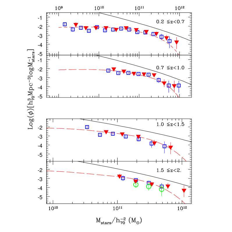
Figure 8: Observed Galaxy Stellar Mass Functions in the K20 sample, compared with the baryonic mass function in a $\Lambda$–CDM hierarchical scenarios and with PLE predictions for the galaxy stellar mass function. The redshift ranges and symbols are the same as in Fig. 4. In particular, hollow circles represent the stellar mass function computed only on the sample with spectroscopic redshifts. The solid line is the theoretical estimate of the Galaxy Baryonic Mass Function, that is to be regarded as an upper limit in$\Lambda$–CDM scenarios. The dashed line is the GSMF predicted by PLE models.

the mass assembly of galaxies is driven by the merging of DM halos. After initial collapse the latter coalesce to form larger and larger structures (from galaxies and small groups to rich clusters of galaxies), at a rate well approximated by the Extended Press & Schechter theory (Lacey & Cole 1993, and references therein).

Thus, galaxies are included into progressively larger and larger host DM structures, where they may merge with the central dominant galaxy due to dynamical friction, or undergo binary aggregations with other galaxies orbiting the same host halo. The analytic description of these dynamical processes is bound by an a posteriori consistency with high resolution N-body simulations. Once these processes have been fixed, the distributions of galaxies as a function of their DM circular velocity can be computed without further ambiguity, and is only slightly dependent on the assumptions used to describe the dynamical processes involved. Assuming that baryons smoothly follow the DM condensations, one can then derive the expected distributions of the available baryonic galaxy masses that corresponds to the mass distribution of the DM halos. This is obviously an upper limit to the actual GSMF. We have obtained such baryonic mass distributions from the theoretical distribution of galaxy Dark Matter circular velocities (from Menci et al. 2002, Fig. 3), by first computing the corresponding DM mass as $M_{\rm DM}=v_{c}^{3}/10\,G\,H(z)$, where $v_{c}$ is the circular velocity of the galaxy DM halo and $H(z)$ is the Hubble constant at redshift $z$, and then applying a simple scaling $M_{\rm baryon}=M_{\rm DM}\frac{\Omega_{\rm baryon}}{\Omega_{\rm DM}}$, with $\frac{\Omega_{\rm baryon}}{\Omega_{\rm DM}}=\frac{0.045}{0.23}$ from the best-fit WMAP parameters (Bennett et al. 2003), under the assumption that $\frac{\Omega_{\rm baryon}}{\Omega_{\rm DM}}$ is constant down to galactic scales. As discussed above, there are essentially no free parameters in deriving these distributions, that depend primarily on the cosmological parameters and on the dynamics of galactic sub-halos. These constitute at present the most solid description of the hierarchical galaxy formation models, so that the predicted distribution of $M_{\rm baryon}$ can be considered as a solid upper bound to the observed GSMF.

The resulting distributions are then compared in Fig. 8 with the empirical K20 stellar mass distributions. The observed number density of massive galaxies never exceeds this fundamental $\Lambda$–CDM constraint. This is equivalent to say that at all explored redshifts there are enough massive DM halos to account for the observed comoving number density of massive (in $M_{*}$) galaxies (see also Gao et al. 2003). There is a tendency for the most massive galaxies at $z\lower 2.15277pt\hbox{$\;\buildrel<\over{\sim}\;$}1$ to be somewhat close to this limit but, as discussed in Sect. 5, this may be due to the impact of large scale structures in our sample. From Fig. 8 one derives that massive galaxies have already converted into stars $\sim 30-50\%$ of the available baryon reservoir, and therefore have a ratio $M_{\rm DM}/M_{*}\simeq 10-20$, consistent with the observed properties of local massive ellipticals (Padmanabahn et al. 2003). This efficiency of baryon-to-star conversion drops rapidly with decreasing mass of the host DM halo, in agreement with the naive expectation that star formation can proceed to a higher level of completion in deep potential wells, while early winds or other effects easily evacuate of most of their baryons the less massive DM halos with shallower potential wells. Several interesting ramifications may follow from this semi-empirical estimate of the baryons-to-star conversion efficiency as a function of the mass of DM halos, but following them in any detail goes beyond the scope of the present paper. We just notice here the relevance of this aspect for the chemical evolution of galaxies, the IGM and the ICM, the run of the total mass to light ratio as a function of galaxy mass, etc.

Another kind of constraint can be obtained from the Pure Luminosity Evolution (PLE) models: by neglecting any merging, and requiring consistency with the properties of present-day galaxies, these models provide an upper limit on the stellar mass distribution within a given cosmology. We have estimated the GSMF evolution for the PLE case starting with the local $K$-band luminosity function for the various morphological types (Kochaneck et al. 2001), and by evolving back in time the mass of each galaxy according to the e-folding time of the star formation rate appropriate for the corresponding morphological types (Pozzetti et al. 1996, 1998). The full procedure is described in Paper V of this series (Pozzetti et al. 2003), and the resulting PLE predictions are shown in Fig. 8. At $z\leq 1$, these predictions are in excellent agreement with the observed data, with the possible exceptions of the more massive bins, where there appears to be an excess of galaxies in the data with respect to the PLE prediction. However, in the two bins around $z=0.7$ most of the contribution to the top end of the GSMF comes from the prominent concentrations (clusters) at $z=0.67$ and 0.73. At higher redshifts, the PLE predictions are still well consistent with the data. At $z=1.5-2$, PLE models are formally above the observed density by about 30% around $M_{*}\simeq 10^{11}M_{\odot}$ (see also Fig 10), where the statistics is good and the results of the spectroscopic sample matches the photometric one.

Overall, we conclude from this comparison that the evolution of the massive galaxies in the K20 sample is consistent with the fundamental constraints of the $\Lambda$–CDM scenario, and that the more massive galaxies have already converted into stars a significant fraction of their baryonic reservoir. The actual success (or lack of) encountered by theoretical models in populating the various DM halos with the observed amount of stars is discussed next.

6.2 Comparison with theoretical models of galaxy formation

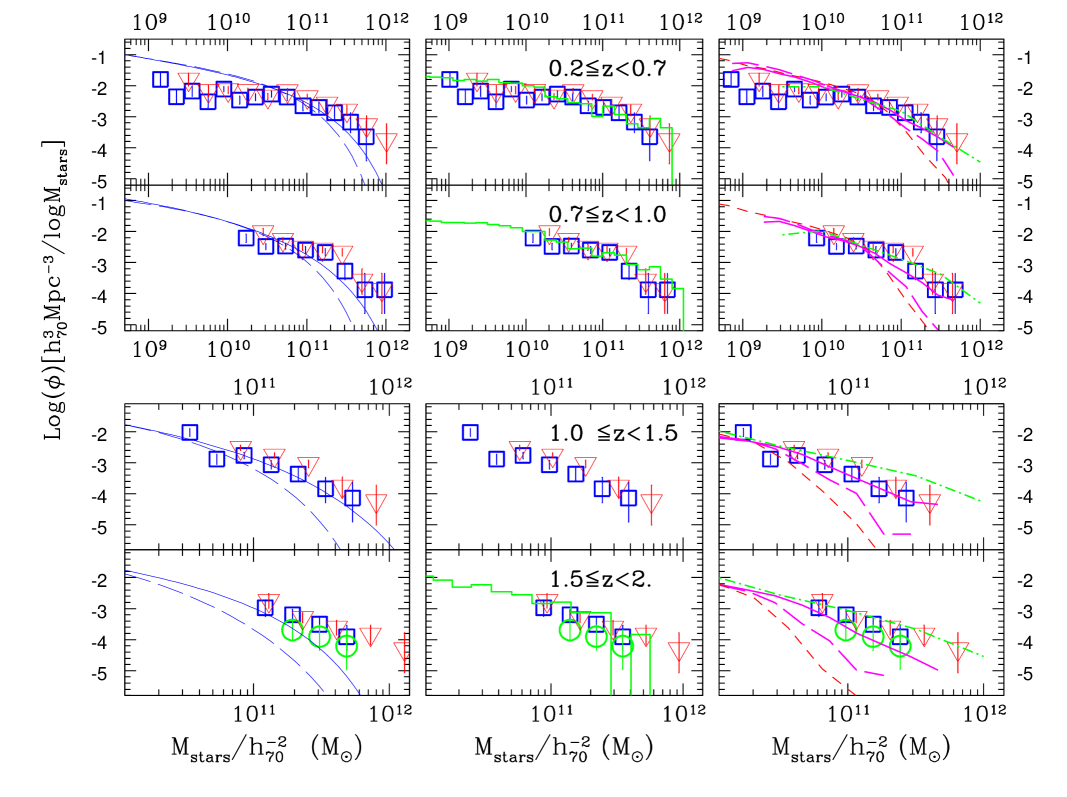
Figure 9: Observed Galaxy Stellar Mass Functions in the K20 sample, compared with theoretical rendition in a $\Lambda$–CDM hierarchical Universe, divided according to the IMF adopted in the models. Left panel: Salpeter (1955), Central panel: Gould et al. (1996), Right panel: Kennicutt (1983). In the central and right panels the observed GSMFs have been scaled to the corresponding IMF as described in the text. The theoretical models are: left panel: Menci et al. (2002) (dashed line) and Menci et al. (2004) (solid line); central panel: Nagamine et al. (2001); right panel: Cole et al. (2000) (short-dashed); Somerville et al. (2004a) (S04 and S04b, thick solid and dashed lines); Granato et al. (2004) (dot–dashed). See text for full details. All the model predictions are evaluated at the central redshift of each bin, with the exception of the Nagamine et al. (2001) case which is computed at $z=0.5$, 1 and 2.

Within the $\Lambda$–CDM scenario, several attempts have already been made to model the history of star formation within DM halos, that is far more uncertain than that of the DM component because of the highly non-linear behavior of the baryonic component.

A first class of theoretical models have been developed using simple parametrized prescriptions to relate the star-formation rate to the properties of such halos, without attempting a physical modeling of the baryonic component. These semi-analytical models (SAM) include e.g., those of Cole et al, (2000), Somerville et al. (2001), and Menci et al. (2002,2004).

Another class of models are those complementing N-body simulations for the dissipation-less components (DM and stars) with a full hydro-dynamical description of the baryonic gas component: we shall consider in the following the simulation of Nagamine et al. (2001a,b) based on the Cen & Ostriker (2000) models.

Finally, Granato et al. (2004) presented a semi-analytical type model, focused on the relationship between the early formation of AGNs and spheroids.

We shall proceed in this section to a comparison of the K20 results with these theoretical models. Fig. 9 displays in separate panels the direct comparison of the various model GSMFs with their K20 counterparts. As an alternative approach, we provide another comparison with the theoretical models in Fig. 10, where we plot the evolution the stellar mass density contributed by galaxies in the range $5\times 10^{10}M_{\odot}\leq M_{*}\leq 5\times 10^{11}M_{\odot}$ (i.e., around the Schechter mass in the local mass function of Cole et al. 2001) which in the K20 sample can be computed with at most little extrapolations of the GSMF.

In making this exercise, we had to compensate for the different IMF adopted in some of the theoretical models. This has been accomplished by applying the appropriate scaling factor to our GSMF and stellar mass densities, as described below.

6.2.1 Semi-analytical models

The main differences among the SAMs considered in this section concern the physical descriptions of processes such as the interactions among satellite galaxies orbiting the same host DM halos (groups or clusters), the star formation processes during galaxy interactions and merging events, the baryonic fraction, and the adopted stellar IMF. On the other hand, they all adopt the same standard parametric laws for the “quiescent” star formation and the supernova feedback. In particular, we shall consider the following SAMs:
M02) The SAM by Menci et al. (2002) with assumptions largely similar to the C00 model. The main difference is that interactions among satellites are now considered to affect only the mass distribution of galaxies when the orbital parameters are conducive to bound mergers. It adopts $\Omega_{b}=0.03$, and a Salpeter IMF.
M04) The “interaction starburst” model by Menci et al. (2004): in addition to the processes considered in the M02 model, it includes the effects of fly-by galaxy interactions (not leading to bound merging) as triggers for starbursts. The cross section and the burst efficiency are taken from the physical model for the destabilization of gas during galaxy encounters developed by Cavaliere & Vittorini (2000). This approach leads to a higher average contribution of starbursts with respect to the S04a and S04b models (see below).
C00) The SAM of the Durham group, in the Cole et al. (2000) rendition (see also Baugh et al. 2003). In this model, the interactions between satellite galaxies are not considered to affect either the mass distribution of galaxies or their star formation in a direct fashion. The model also adopts a low value of $\Omega_{b}=0.02$ and a Kennicutt IMF.
S04a) The “merging starburst” model of Somerville et al. (1999, 2001) in its recent rendition (Somerville et al. 2004a), which includes the effects of merging between galaxies on both their mass function and their star formation rate, the latter being bursted in each merging event. The cross section and the burst intensity are derived by extrapolating the results of hydro-dynamical N-body simulations to the whole range of masses considered in the model. In this model $\Omega_{b}$ is 0.04 and a Kennicutt IMF has been adopted.
S04b) A “reduced merging” version of S04a, that has been used to compare the predicted redshift distribution for $K_{s}\leq 20$ with the K20 and GOODS data (Somerville et al. 2004b). Among the major revisions, this “reduced merging” recipe has been adopted by increasing the Dynamical Friction time and adding an additional time delay for halo relaxation (see e.g. Mathis et al. 2002). In practice, this model has the same star–formation recipes of S04a but a reduced formation of massive objects.

To put both the latter three models and the K20 GSMFs on the same foot, the observed masses have been systematically reduced by 0.35 dex. No such reduction is necessary when comparing with the M02 and M04 models, since they were constructed adopting the Salpeter IMF.

In the low-redshift bin all the SAM mass functions appear to be systematically steeper than the observed GSMF, with a pronounced excess of low-mass galaxies, and an incipient deficit of massive ones. The former discrepancy is a well known problem afflicting some SAMs also at zero redshift (e.g., Cole et al. 2000; Baugh et al. 2002), which is also directly noticeable in the comparison of the luminosity functions from UV to IR (Poli et al 2001, Pozzetti et al. 2003, Poli et al. 2003).

Fig. 9 shows that most SAMs do reproduce the bulk of the GSMF (i.e. the region around $M_{*}$), although they often under-produce the very massive galaxies by an amount that increases with redshifts. Moreover, the various models show a remarkably large spread in the predicted GSMF, and progressively diverge from each other with increasing redshift, reaching differences by more than 2 orders of magnitudes at the highest explored redshifts.

The same results can be obtained by looking at the evolution of the stellar mass density of galaxies in the range $5\times 10^{10}M_{\odot}\leq M_{*}\leq 5\times 10^{11}M_{\odot}$ (Fig. 10). It is worth noting that a significant decrease ($\sim 50\%$ from $z=0$ to $z=2$) is exhibited also by the PLE models, despite the large $z_{\rm form}=5.7$ adopted.

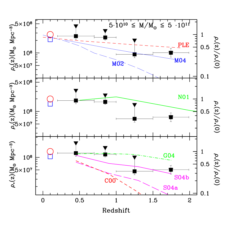
Figure 10: Cosmological Stellar Mass Density for objects of $M_{*}\simeq 10^{11}M_{\odot}$ in the K20 survey, compared with the theoretical models discussed in the text, divided according to the relevant IMF: upper panel: Salpeter (1955), central panel: Gould et al. (1996), lower panel: Kennicutt (1983). Filled squares represent the BF estimates, filled triangles the MA estimates. The empty circle at $z=0.1$ represents the local value of Cole et al 2001, the empty square the same value “scaled” to BF (see text for details). The models plotted are: Menci et al. 2002 (M02, long dashed line), Menci et al. 2004 (M04, solid line) and PLE (short–dashed line) in the upper panel; Nagamine et al. 2001 (N01, solid line) in the central panel, and Cole et al. 2000 (C00, short-dashed); Somerville et al. 2004a (S04a and S04b, thick solid and dashed lines); Granato et al 2004 (dot–dashed line). See text for more details. The relative value with respect to the local value of Cole et al. 2001 is shown in the right y–axis.

Given the complexity of the baryonic physics involved in galaxy formation, all the parameterizations adopted by the various SAMs appear a priori equally plausible. Yet, as shown by Fig. 9 and Fig. 10, the results diverge dramatically with increasing redshift, offering a rather powerful opportunity for the direct observation of high redshift galaxies to discriminate between more or less viable SAMs, thus possibly giving useful hints for a better understanding of the dominant physical processes. For example, it appears that merging- or interaction-induced starbursts may be an essential ingredient in order to produce a number of massive galaxies at $z>1$, approaching the corresponding number that this survey has detected. On the other hand, the standard, ”quiescent” star formation regulated by the cooling time of baryons within the DM halos (as adopted e.g., in C00 and M02) appears to produce the most discrepant results compared to the observations presented in this paper. Also, the comparison suggests that the standard recipes for dynamical friction adopted by S04b and M04 tend to perform better than the “reduced” merging treatment (S04a), that was introduced to improve the match with the density of bright galaxies in the local universe.

6.2.2 N-body/hydrodynamical models of galaxy formation

Unlike SAMs, the Nagamine et al. (2001a,b) simulation dynamically solves a full set of fluid equations for baryons, and includes physical processes such as radiative cooling and heating of the gas, star formation, and supernova feedback, with star particles being created out of the gas where it is contracting and cooling rapidly. To some extent, the effect on star formation of galaxy interactions is also automatically included in these simulations.

The published versions of these models provide GSMFs only for redshift bins centered at $z=0.5$, 1, and 2, that we compare in Fig. 9 with the empirical K20 GSMFs in the $0.2<z<0.7$, $0.7<z<1.0$ and $1.5<z<2$ redshift bins, respectively. Since these models adopt the IMF from Gould et al. (1996), the K20 masses have been systematically scaled down by a factor 0.72, which is the appropriate correction to take into account to convert them to a Salpeter IMF (Nagamine, private communication).

Fig. 9 shows that these models predict an evolution of the GSMF that is in very good agreement with the K20 results, avoiding both the low-mass excess and the high-mass deficit typical of SAMs. The good agreement in the low-mass range is likely to be due to the stronger feedback effect that in these models is tuned to match the X-ray background, resulting from the AGN activity.

Fig. 10 shows that the Nagamine et al. models also predict a very mild decrease with $z$ of the high-mass contribution to the stellar mass density, actually even milder than that derived from the K20 data. We note also that these models predict that $\sim 30\%$ of the stellar mass is already in place by $z=3$ (Nagamine et al. 2004), in agreement with the expectation from the so-called “fossil evidence” (Renzini 1998, 2003).

6.2.3 Models for the joint evolution of QSO and spheroidal galaxies.

Yet another class of models has been developed specifically to explore the mutual feed-back between star formation in spheroids and the high-z QSO activity (Granato et al. 2001, 2004), largely neglected by classical SAM. In the latter paper, dark matter halos form at the rate predicted by the canonical hierarchical clustering scenario, and processes such as collapse, heating, cooling and supernovae feed-back are taken into account with techniques and recipes typical of other SAM. However, (i) it is assumed that angular momentum plays a negligible role in slowing down star formation activity in massive halos virialized at high redshift, which would be those leading to spheroid formation and are the only one accounted for in this model; (ii) the growth by accretion of a central SMBH is promoted by the resulting huge, and heavily obscured, star formation rate and (iii) the feed-back on the ISM due to the ensuing AGN activity is taken into account with recipes inspired by the physics of Broad Absorption Line QSOs.

This model adopted a double–slope IMF that provides a $M_{*}/L$  ratio very close to Kennicutt. For this reason, we will plot this curve in the same panel with the Kennicutt models. We note that in the case of the second redshift bin ($0.7<z<1$), the model has been computed at $z=1$, and should therefore be considered as slightly underestimated.

The comparison with the K20 data suggests a good agreement in the $z\leq 1$ range, and an overestimate of a factor about 2 of the mass density of massive galaxies at $z>1$. In this redshift range, this models predicts a fraction of massive galaxies to be strongly extincted, and therefore to escape our $K<20$ selection criteria: further modeling is required to assess whether this effect is able to reconcile the model with our observations.

7 Summary and Discussion

In this work, we have used the spectroscopic redshifts and the spectrophotometric properties of the galaxies in the K20 sample to estimate their stellar masses and to build the corresponding GSMF at different redshifts. Our basic results, that are based on the assumption of a Salpeter IMF, can be summarized as follows:

$\bullet$ We have used two different methods to estimate the stellar mass $M_{*}$ and the rest-frame luminosities for each galaxy in the sample. In one case, we assume all galaxies started to form stars at $z=20$ with a star-formation rate declining exponentially thereafter. The e-folding time is then determined by demanding the stellar population model to reproduce the observed $R-K$ color. We referred to this approach as the “Maximal Age” (MA) method. In the other approach, we remove any constraint on age, metallicity and dust content, but require consistency with the whole multicolor spectral energy distribution. We referred to this approach as the “Best Fit” (BF) method.

$\bullet$ Wehave performed a comparison of the two methods, showing that the typical BF masses are lower with respect to the MA estimates by a factor that is typically $\simeq 2$ for objects of $M_{*}=10^{10}M_{\odot}$ and $\simeq 1.5$ for objects of $M_{*}=10^{11}M_{\odot}$. This lower estimate is due to the lower galaxy age obtained on average from the BF procedure. We have also carefully inspected for systematic effects by means of simulations, comparison with the spectroscopic information and by looking at the intrinsic degeneracy among the input parameters. We conclude that the two methods together should give a fair representation of the existing uncertainties in the derived masses.

$\bullet$ The final galaxy sample of the K20 survey spans a range of stellar masses from $M_{*}=10^{9}M_{\odot}$, at the lowest redshifts, to masses close to $M_{*}=10^{12}M_{\odot}$. Such massive galaxies appear to be common at $0.5<z<1$, and are detected up to $z\simeq 2$.

$\bullet$ With the K20 data set, we have built the Galaxy Stellar Mass Function (GSMF) and the corresponding total mass density in four redshift bins centered at $z=0.45,0.85,1.25,1.75$, while introducing a correction to take into account for the incomplete coverage of faint objects with high $M_{*}/L$ .

$\bullet$ Up to $z\simeq 1$, we observe only a mild evolution of the GSMF and of the corresponding global stellar mass density. Both the MA and the BF estimated GSMFs indicate a decrease by $\sim 20-30\%$ of the number density of objects around $10^{11}M_{\odot}$ (where the statistics is sufficiently accurate). This implies that the evolution of objects with mass close to the local characteristic mass is essentially complete by $z\simeq 1$.

$\bullet$ At higher redshifts a drop begins to appear in the comoving number density of galaxies within the explored mass range, corresponding to a decrease in the normalization of the GSMF. At $z\simeq 2$, a fraction of $\sim 30-40\%$ of the present day stellar mass in objects with $5\times 10^{10}M_{\odot}<M_{*}<5\times 10^{11}M_{\odot}$ appears to be in place.

$\bullet$ We detect a change in the physical nature of the most massive galaxies: at $z\lower 2.15277pt\hbox{$\;\buildrel<\over{\sim}\;$}0.7$, all galaxies with $M>10^{11}M_{\odot}$ are either early or early$+$emission type, while the mass density due to massive star–forming galaxies increases with $z$: in the highest redshift bin, we estimate a lower limit (due to incomplete spectroscopic identification) of 21% to their contribution to the observed stellar mass density.

$\bullet$ The observed evolution of the $M_{*}/L_{R}$  ratio (Sect. 4.2) provides evidence for a differential evolution of early type galaxies, suggesting that more luminous (i.e. more massive) galaxies appear to reach near completion first, while less massive ones keep growing in mass till later times. A direct detection of this effect in our GSMF is hampered by the low statistics, although we note that there is a tentative indication that the decrease with redshift of the GSMF is more pronounced towards the low-mass end of the explored range than for the most massive objects. Clearly, much wider surveys are required to confirm this potentially crucial item.

$\bullet$ The global rise of the stellar mass density from $z\simeq 3$ to $z\simeq 1$ is broadly consistent with the integrated contribution from the global star–formation as inferred from UV–selected galaxies, once a modest amount of dust extinction (E(B-V)=0.15) is accounted for.

$\bullet$ It is shown that the large number of massive galaxies detected at high $z$ does not violate any fundamental $\Lambda$–CDM constraint. Specifically, up to $z=2$ there is no shortage of DM halos massive enough to account for the baryonic mass of the observed galaxies. Very interestingly, the fraction of baryons converted into stars appears to strongly increase with the mass of the host DM halo.

$\bullet$ We have compared in some detail these results with the expectations of updated models for galaxy formation in a $\Lambda$–CDM Universe, including several ab initio renditions, either semi-analytical (namely: Cole et al. 2000; Somerville et al. 2004a,b;; Menci et al. 2002, 2004) or hydrodynamical simulations (Nagamine et al. 2001a,b), as well as the physically motivated model of joint evolution of QSO and galaxies by Granato et al. (2001,2004). The predicted evolution of the GSMF varies quite dramatically from one rendition to another, being very sensitive to model ingredients such as interaction-driven starbursts, feedback, etc. Some semi-analytical models are consistent with the observations up to $z\simeq 1.5$, and slightly underestimates those at higher $z$, while other underpredict, in some case by a large factor, the number density of massive galaxies at high redshift. Conversely, the hydrodynamical simulations of Nagamine et al. (2001a,b) and the Granato et al. (2004) models appear to match the observed number density at $z\simeq 1$, where they equal or even exceed the PLE predictions, and even overpredict the ones up to $z\simeq 2$. It is worth noting that the strong contribution of AGNs to the feedback in the models of Nagamine et al. (2001a,b) and Granato et al. (2001, 2004) is apparently effective in order to suppress star formation in low-mass halos at early times, and to reproduce the slope of the GSMF at low masses. On a different line, the PLE predictions appear to be consistent with the observed data, at least up to $z=1.5$.

$\bullet$ We have accompanied all these findings by several cautionary remarks concerning their sensitivity to the adopted IMF, and possible biases due to surface brightness dimming effects, highly obscured objects, the narrowing range of explored masses at high redshift, and cosmic variance.

While keeping these caveats in mind, the present results allow to sketch a global scenario for the evolution of massive galaxies. Up to $z\simeq 1$, clearly little evolution has taken place in these objects. Their number density is close to the local one ($\sim 70-80\%$) and to the prediction of simple PLE models. In addition, most of the mass density resides in early-type, passively evolving galaxies, that must have formed the bulk of their stars at least $2-3$ Gyr before, i.e., at $z\lower 2.15277pt\hbox{$\;\buildrel>\over{\sim}\;$}2$. In this respect, the K20 survey strengthens similar conclusions by Brinchmann & Ellis (2000), using the CFRS data (Lilly et al. 1995), by D03 and F03 in the much smaller HDF fields. The stability of the massive, early type galaxy population up to this redshift is also recovered by the COMBO17 Survey (Bell et al. 2004), accompanied by a progressive disappearance of the less massive early-type (red) galaxies.

Beyond $z\sim 1$ the evolution of massive objects starts to accelerate and by $z\simeq 1.8$ $\sim 30-40\%$ of the local density has been locked in massive galaxies. This is associated with a change in the physical properties of massive galaxies, among which star-forming objects now become common, and contribute a much more substantial fraction of the observed mass density (at least 21% in the K20 sample). So, several massive $K<20$ galaxies in the high-redshift tail ($z\geq 1.7$) of the redshift distribution are star-bursting objects showing irregular morphologies, and may be strongly clustered (Daddi et al. 2004a), which makes them likely progenitors of local massive early-type galaxies. While up to $z\sim 1.5$ PLE models still give an acceptable fit to the data, at higher redshifts the massive starbursts in the sample mark a departure from such models, and signal that one may be entering the formation epoch of massive spheroids (Daddi et al. 2004; Somerville et al. 2004b). However, with the K20 survey we have got just a first glimpse to the transition from the passively-evolving to the active star-forming progenitors of the local early-type galaxies. Wider areas and deeper spectroscopic surveys are clearly required to thoroughly map this transition, that may extend up to $z\sim 3$ and beyond.

Overall, these features are in agreement with the basic elements of the $\Lambda$–CDM scenarios. In an accelerating universe, massive galaxies have time to complete their assembly at $z\simeq 1$, avoiding too much merging at low redshifts. Thanks to the availability of gas, shorter cooling time, and higher interaction and merging rates star formation naturally occurs most efficiently at earlier times. The anti-correlation of feedback with the halo mass, and the correlation between high density peaks, boosts the star–formation rate in high mass objects at high $z$, with respect to lower mass ones. Despite these “built in” features, most renditions of the $\Lambda$–CDM paradigm tend to delay the star formation and assembly of massive galaxies well beyond the epochs favored by the present observations, and several of them significantly fail to match the observed mass densities. The reason is tied to the different physical processes that are contained - or ignored - in the models and to the way they are described.

At the time of writing, the Spitzer satellite is acquiring its first data: it is easy to predict that it will bring new, decisive information in this critical issue.

The $M_{*}/L$ ratio, stellar mass densities and GSMFs described in this papers are available in electronic form at the web site http://www.arcetri.astro.it/^∼k20

Appendix A: Validating the “Best Fit” method

A.1 Comparison between the Maximal Mass and Best Fit mass estimates

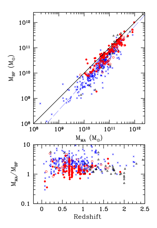
Figure 11: Comparison between the stellar masses estimated for the K20 galaxies with the Maximal Age and Best Fit techniques. Upper panel: The relation between MA (x–axis) and BF (y–axis) stellar masses in the K20 sample with full multicolor coverage. Different symbol refer to spectroscopic classification, as in Fig 1: solid circles, early type; empty circles, early+emission type; crosses, late type; triangles, photometric redshifts. The dashed line shows the first–order fit to the observed relation. Lower panel: Ratio between the MA and BF sample as a function of the redshift, for the same sample. Symbols have the same meaning of the upper panel.

Figure 11 shows the comparison between the stellar masses estimated with the two different criteria. Beyond the obvious correlation, it is immediately clear that the MA models provide an estimate that is typically larger than the BF estimates, although a large scatter exist. The ratio between the two methods is larger at intermediate masses, and it is on average a factor $<M_{\rm MA}/M_{\rm BF}>\simeq 2$ at $10<log(M_{\rm BF}/M\odot)<10.6$, and converges toward a factor $<M_{\rm MA}/M_{\rm BF}>\simeq 1.6$ at $log(M_{\rm BF}/M\odot)>10.6$. We have found that this difference is mainly due to the lower average ages that are inferred for the K20 galaxies in the BF approach (the median $z_{\rm form}$ resulting from the “BF” approach is about 2). We have verified that this trend still holds if we fix the metallicity to a solar value, or if we use different extinction curves, like e.g. Calzetti 2000. A few BF models have larger stellar masses than the corresponding MA estimates: these results from objects fitted with large ages (comparable with the MA assumptions) and with combinations of dust and/or metallicities that further enhance the $M_{*}/L$ ratio. We also note that a contribution to the scatter (with a 10% r.m.s.) results from the different normalizations (see Sect. 3.3).

We have obtained a simple first order regression to the points in Fig. 11, finding that the relation $logM_{\rm BF}=1.106(\pm 0.001)\times(logM_{\rm MA})-1.42(\pm 0.06)$ provides a reasonable fit to the observed relation, accurate to $\Delta logM_{*}\simeq 0.14$.

A.2 The effect of secondary bursts

Figure 12: Results of the simulations performed to check the reliability of the Best Fit stellar mass estimates in the cases of star–formation histories characterized by multiple starbursts. The histogram shows the ratio between the fitted mass $M_{\rm fit}$ and the input one $M_{\rm input}$ at three different ages of the second starburst. The solid line shows the results of the simulations done assuming that the second starburst assembles a fraction $f$ from 10% to 70% of the total mass. Thin solid line is the simulation with $f=10$%. Dashed line shows a simulation with the starburst component only.

In order to check the reliability of the BF stellar masses estimates, in particular during secondary starbursts, we have performed a set of simulations. We have computed a mock multicolor sample assuming a scenario where galaxies were built during two major starbursts. During the first one, characterized by an initial redshift $z_{\rm form1}$ and exponential timescale $\tau_{1}$, a fraction $1-f$ of the total final mass is assembled. All possible permutations of $z_{\rm form1}=10,8,6,4,3,2.5$, $\tau_{1}=0.1,0.3,1,5$ Gyrs were adopted, to ensure a proper sampling of any spectral type, including very red, passively evolving galaxies. Solar metallicity and no dust was assumed in this case. In addition, a younger starburst was summed, contributing for a fraction $f$ of the final mass, with star–formation time scales $\tau_{2}=0.1,0.3,1$ Gyrs and ages $0.1,0.2,..2$ Gyrs. Solar metallicity and $E(B-V)=0.2$ was adopted. The resulting mock spectral distributions were computed with $f=0.1,0.3,0.5,0.7$ at $z=0.5,0.6...1.3$ to cover the main range of our observations, and were analyzed with the same recipe of the K20 sample. In Fig12 we show the histogram of the recovered stellar mass $M_{\rm fit}$ with respect to the input one $M_{\rm input}$, at different starburst ages. It is shown that if the second burst is caught during its early phase, within the first $0.2-0.3$ Gyrs from its start, the BF estimated mass is typically lower than the actual one by a factor of about 25% (average value). We have found that the effect is larger when the fraction $f$ is small (as shown from the $f=0.1$ case in the histogram of Fig12) and/or the first starburst is peaked at high $z$. At larger ages, the BF estimated mass approaches the input one, leading to a final average underestimates of 20% at a starburst age of 1 Gyrs and only 10% after 2Gyr. As a check,we have also verified that if we include only single exponential laws (dashed line in Fig. 12) the resulting fit is essentially unbiased.

These simulation show that if the observed galaxy have a star–formation history significantly departing from single exponential, and are observed during a major starburst, the overall effect on the estimate of the stellar mass is relatively small, especially for the reddest galaxies, that dominate the massive tail of the GSMF.

A.3 The D4000 break

Figure 13: Comparison between the D4000 break measured from the K20 spectroscopic observations (x axis) and the D4000 break estimated from the Best Fit models (y axis). Filled dots represent late–type galaxies while crosses the star–forming ones.

The $D4000$ break is known to be a sensitive probe of the age of the underlying stellar population, and as such is a precious information to test the star formation scenario that is produced by the BF models.

We plot in Fig. 13 the comparison between the $D4000$ break measured from the K20 spectroscopic observations and the $D4000$ break estimated from the Best Fit models. The comparison shows a relative good agreement, with a nearly null average difference (that is $\Delta D4000=0.02$) and a dispersion of 0.2, that is smaller than the average error on the spectroscopic $D4000$. Fig. 13 shows that, as expected, the $D4000$ break of early–type galaxies is pretty larger than for later types. In particular, we have found that the average $D4000$ of the “old” EROs population, derived from BF models, is very close to the value of the average spectrum, that is 1.9 (Cimatti et al. 2002c).

A.4 Quantifying the internal degeneracies

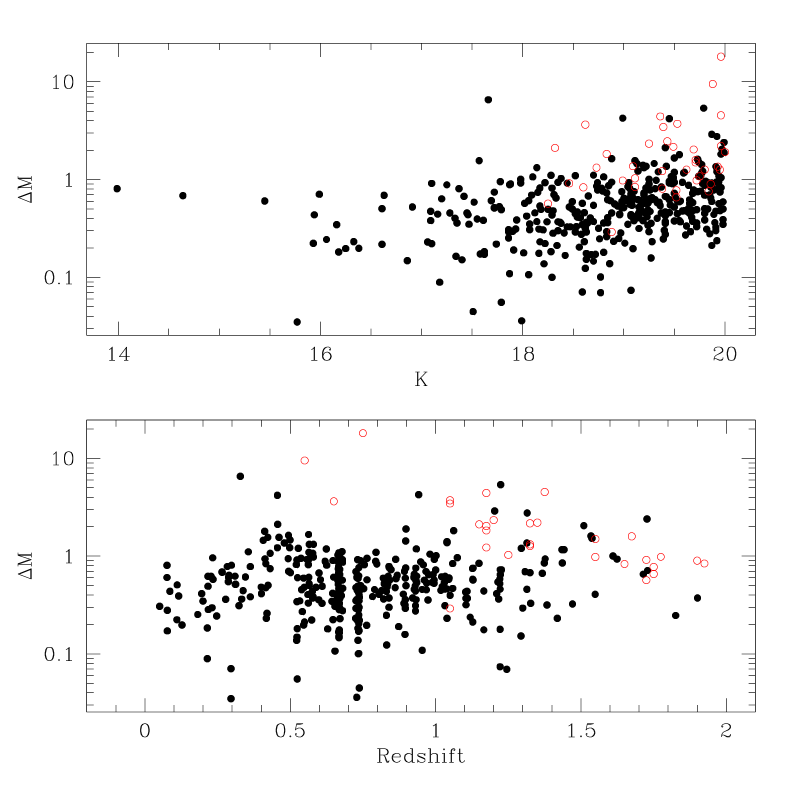
Figure 14: Confidence levels on the estimated BF mass, as a function of $K$–band magnitude (upper panel) and redshift (lower panel). The confidence level $\Delta M_{*}$ is defined as $\Delta M_{*}=(M_{\rm max}-M_{\rm min})/2M_{\rm best}$ Filled points represent objects with spectroscopic redshift, empty with photometric redshifts.

Given the wide range of the free parameters involved in the BF estimate, and the relatively loose constraints that can be obtained from broad band imaging only, the best fit solution to each galaxy is far from being univocal. An advantage of the $\chi^{2}$ approach is that it allows to take into account the resulting degeneracies among the input parameters adopted and to provide an estimate of the range of “acceptable” models. At this purpose, we use a technique already adopted in F03, and similar to the one adopted by Papovich et al. 2001, based on the reduced chi–square $\chi^{2}$ (as computed in Fontana et al. 2000). The $1\sigma$ confidence levels on the fitted parameters (such as mass, age and star–formation rate) have been obtained by scanning the model grid and retaining only the models that have $\chi^{2}\leq\chi^{2}_{\rm bestfit}+1$. Prior to this, as in Papovich et al. 2001, we have rescaled the noise in bright objects order to have $\chi^{2}_{\rm bestfit}=1$ The scan is performed either at fixed redshift (for objects with known spectroscopic redshift) or allowing the models to move around the best–fitting photometric redshift.

In general, the range of acceptable values will not be symmetric with respect to the best–fit solution: we find that the typical range for a galaxy of stellar mass $M_{*}$ is $0.6M_{*}-1.6M_{*}$. This uncertainty is in agreement with the similar results in the HDFN (D03) and HDFS (F (03)) at the same redshifts and signals a core level of degeneracy in the input models, that cannot be resolved without detailed spectroscopic informations. This level is lower than the comparable estimates at $z\simeq 3$ (Papovich et al. (2001), Shapley et al. (2001)), since we can rely on a better sampling of the NIR side of the spectrum.

To show how the uncertainty depends on the redshift and observed flux, we use a simplified (symmetrical) estimator computed as $\Delta M_{*}=(M_{\rm max}-M_{\rm min})/2M_{\rm best}$, that we plot as a function of redshift and $K$–band magnitude in Fig. 14. For most of the objects, this estimator is below 1, consistent with the average uncertainty quoted above, showing that our mass estimates are overall robust within a factor of 2. As expected, faintest objects have a typically larger uncertainty, as well as objects with $z>1.5$, that begin to suffer from the poor sampling of the IR side of the spectrum: longer wavelengths data, as those provided by the recently launched Spitzer satellite, are required to improve their estimates.

Finally, we have found that MA model typically lay close to the upper confidence level. Quantitatively, we have found that about 40% of the MA values are lower than the upper $2\sigma$ confidence level, and that the MA values are on average only 10% larger than the upper $2\sigma$ confidence level.

A.5 The local sample

We address here the impact that our two different techniques to estimate the stellar masses have on the estimate of the local stellar mass functions and density ( Cole et al. (2001)), which are the pivots of the evolutionary trends that we have analyzed. At this purpose, we have followed the procedure described by Bell et al. (2004) to build a sample of local galaxies (i.e. $z\simeq 0.1$) by cross-correlating the SDSS and 2MASS public catalogs. Using a sub area of the SDSS EDR, we obtained a catalog of 6332 galaxies with full $ugrzJHK$ photometry, from which we obtained the MA and BF stellar masses as described in the main text. The main results of this comparisons are:

- MA stellar mass estimates do not depend sensitively on the color adopted. We have tested that using either the $J-K$, as done by Cole et al. (2001), or the $R-K$ (as we did in our sample) or the $G-J$ (that grossly mimics the $R-K$ of our sample) the MA estimates do not change systematically.

- In the local Universe, BF stellar estimates are systematically lower than MA by about 20%, with a trend of decreasing offset for more massive objects. This is shown in fig15, where the two samples are compared. A linear regression between $M_{\rm MA}$ and $M_{\rm BF}$ yields $M_{\rm BF}=1.027\times M_{\rm MA}-0.3955$.

Using the above relation to statistically convert the Cole et al. (2001) mass function to a BF one, we obtain the stellar mass function shown in the lower panel of fig15, that marginally departs from the original of Cole et al. (2001) in the massive tail. Whenever we have analyzed the evolution of the mass density with redshift with our “BF” estimates, we have adopted this “BF–scaled” local mass function to compute the corresponding local mass densities.

Figure 15: A comparison between the stellar masses estimated with the Maximal Age and with the Best Fit methods on 6500 galaxies at $z\simeq 0.1$ taken from the SDSS and 2MASS surveys. Solid line is the $M_{\rm BF}=M_{\rm MA}$ locus, dashed line is the linear regression among the observed points.

Appendix B: Incompleteness effects in the stellar mass function

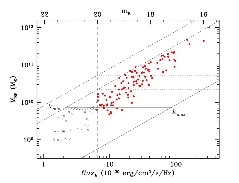
Figure 16: Relation between the observed $K_{s}$ flux (lower scale; in the upper scale, the corresponding $K_{s}$ magnitude) and the BF estimated stellar masses, at $z\simeq 0.7$. Filled points are taken from the K20 sample, empty are taken from the HDFS sample (F (03)) for comparison only. The diagonal lines bracket the whole range of masses that are allowed to galaxies of the corresponding $K_{s}$ magnitude in the BF model grid. The solid line show the minimal mass for objects of given flux. The dashed line is the maximal mass, if one takes into account dusty objects, while the dashed–dotted line is the maximal mass for dust-free, passively evolving objects. The dashed vertical line shows the $K_{s}<20$ limit of the K20 survey. The dotted line show the resulting (strict) completeness limit on stellar masses, according to the selection curve adopted. The shaded area shows the fraction of galaxies lost (at a given mass) by incomplete coverage of the $M_{*}/L$ ratio.

As discussed in the main text, the building of the corresponding stellar mass function follows the traditional techniques ($1/V_{\rm max}$ and Maximal Likelihood) used for luminosity functions, although a treatment must be included to correct for the incompleteness (in mass) at the faintest levels, that arise from the not univocal conversion from the observed K-band to the stellar mass. To emphasize this issue, we plot in figure 16 the stellar masses $M_{\rm BF}$ obtained in the K20 sample at the redshift of $z\simeq 0.7$ as a function of the observed $K_{s}$ flux. The K20 sample is shown with filled points. To ease the visual representation of the incompleteness effect, we add with empty symbols the corresponding points at $K_{s}>20$ from a similar analysis carried on in the HDFS (F03).

The relation follows the expected correlation with a scatter of about $\Delta log(M_{*})\simeq 0.6$, due to the intrinsic scatter in the $M_{*}/L_{K}$ ratios. We note that the $K_{s}=20$ limit cuts the galaxy strip at a mass level that varies from $\log(M_{*}/M_{\odot})=9.5$ to $\log(M_{*}/M_{\odot})=10.3$. The incompleteness at the faint $M_{*}$ levels becomes evident by observing the point distribution at a fixed $M_{*}$ level. At, say, $M_{*}\simeq 8\times 10^{9}M_{\odot}$, about half of the galaxies lay at $K_{s}>20$, and are therefore missed by a $K_{s}\leq 20$ sample. To recover from this incompleteness, one can make use of the distribution of the $M_{*}/L$ ratio, both as expected from the library adopted and as observed in the data, as we describe below.

By construction, the points must lay between the minimum and maximum mass that a galaxy at $z\simeq 0.7$ may have at a given $K_{s}$ magnitude: these limits can be obtained from the model grid that is assumed to describe the galaxy properties. In the case of the BF grid, we have computed these thresholds by scanning the output of the spectral library defined in Table 1, which, as discussed in the text, is particularly sensitive to the effects of dust. We plot in Fig. 16 both the upper limit corresponding to dusty objects (dashed line) as well as the limit corresponding to passively evolving dust–free models (dashed-dotted line). The lower limit (solid line) is in both case resulting from a star–forming, dust-free young population.

Strictly speaking, the sample is therefore complete (in stellar mass) only down to the horizontal dotted lines shown in Fig. 16, that correspond to the maximal mass allowable (at any redshift) for a galaxy of magnitude equal to the faint limit of the sample. In principle, stellar mass functions and other quantities should be computed only on the subsample with $M_{*}(z)\geq M^{*}_{\rm compl}(z)$. At masses smaller than this limit, any magnitude–selected sample will be progressively incomplete, although objects of $M_{*}/L$ will still be detected. We note that this effect has not been taken into account in the local estimates of the GSMF (Cole et al. (2001), Bell et al. (2004)), which may explain the decrease of the local GSMF that is observed in their faintest bins.

However, as shown in Fig. 16, the actual threshold sensitively depends on the choice of this “maximal mass” model, and the strict adoption of a selection criteria would result in the loss of a significant fraction of our sample: for these reasons, we have introduced a correction for incompleteness that both allows to recover a significant fraction of the sample and, using the observed distribution of $M_{*}/L$ , removes the critical dependence on the upper and lower limits.

We also note, with that this formalism, we do not need to include any term similar to the $k$–correction terms used in the computation of standard luminosity functions, since the completeness curve by definition allows to compute the maximum redshift used to estimate $V_{\rm max}$.

We remark that the correction is computed for each galaxy at the corresponding redshift, and that we will use here, at variance with the rest of the paper, the ratio between the stellar mass $M_{*}$ and the observed K–band flux $k$. The correction is computed as follows.

At a given mass $M^{*}_{\rm inf}\leq M_{*}\leq M^{*}_{\rm compl}$, the observed K–band flux $k$ corresponding to a given stellar mass $M_{*}$ is encompassed between two values, named $k_{\rm min}$ and $k_{\rm max}$ here (we have adopted in this case of passively evolving, dust free objects). The key quantity is the fraction $1-f_{\rm obs}$ of galaxies lost by effect of the incomplete coverage of the $M_{*}/L_{K}$ ratio, that reside in the shaded area of Fig. 16: in practice, the correction is based on the computation of the fraction of observed galaxies $f_{\rm obs}$, that will be used to correct for the accessible volume element $V_{\rm max}$.

To show how we compute the fraction $f_{\rm obs}$, let us first define the number density $N(M_{*},k)$ of objects (at redshift $z$) with observed $K_{s}$–band luminosity $k$ and mass $M$: in principle, the fraction $f_{\rm obs}$ (at given $M$) can be estimated from the number density of objects $N(M,k)$ as

$$f_{\rm obs}={\int_{k_{\rm lim}}^{k_{\rm max}}{N(M,k)dk}\over\int_{k_{\rm min}}^{k_{\rm max}}{N(M,k)dk}}$$ (1)

Since the shape of $N(M,k)$ at fluxes fainter than our $K=20$ limit is in principle unknown, we have to assume that the distribution of the $M_{*}/L$ ratio at fixed observed luminosities and at a given redshift is independent of the luminosity: although such a factorization (i.e. the assumption that the distribution of the $M_{*}/L$ ratio is independent of the luminosity) does not likely hold at any $k$, we actually need it to be valid around our $K=20$ limit, where we compute our correction. Given the small range in luminosity that we sample around the limit, we do not expect this assumption to invalidate the computation of the correction.

In this case the number density $N(M,k)$ can be written as

$$N(M,k)=\mu(\frac{M}{k})\phi(k)$$ (2)

where $\mu(M/k)$ is the distribution of the $M_{*}/L$ ratio, and $\phi(k)$ is the luminosity distribution of objects with given $M_{*}/L$ . $\phi(k)$ is linked to the luminosity distribution $\Phi(k)$ (i.e. to the galaxy counts of objects at redshift $z$) by the requirement that

$$\Phi(k)=\int_{0}^{\infty}{\phi(k)\mu(M/k)dM}\propto\phi(k)k$$ (3)

.

We have estimated $\Phi(k)$ on our data in the four redshift intervals that we have used, and found that (at $18<K<20$) it can be well represented by a power law :

$$\Phi(k)\propto k^{-2.5\alpha_{z}-1}$$ (4)

with a redshift-dependent index $\alpha_{z}=0.2,0.2,.0.33,0.38$ at $z=0.45,0.9,1.3,1.75$, that is consistent with the overall slope of the counts (dlogN/dK=0.28) from Saracco et al. 2001.

The simplest approach would be to assume that the distribution function $\mu(M/k)$ is constant at fixed $k$ : with this very coarse assumption the correction factor $f_{\rm obs}$ becomes

$$f_{\rm obs}(z,M)={\int\limits_{k_{\rm lim}}^{k_{\rm max}}{k^{-2.5\alpha_{z}-2}dk}\over\int\limits_{k_{\rm min}}^{k_{\rm max}}{k^{-2.5\alpha_{z}-2}dk}}={k_{\rm max}^{-2.5\alpha_{z}-1}-k_{\rm lim}^{-2.5\alpha_{z}-1}\over k_{\rm max}^{-2.5\alpha_{z}-1}-k_{\rm min}^{-2.5\alpha_{z}-1}}$$ (5)

.

Alternatively, one can explicitly take into account the intrinsic distribution in the $M_{*}/L$ ratio. We have already made the assumption that the distribution $\mu(M/k)$ is independent of $k$, at a given $z$, which implies that at the same $z$ the distribution of $M/L$ is independent of $L$, where L is the rest frame luminosity in the wavelength range corresponding to the redshifted K band. We will further assume that the distribution of $M/L$ is also constant within each redshift bin, and that within the redshift bin we can ignore the differential $k$–correction (that are indeed small in the K band (Pozzetti et al. 2003). That is, we assume that one can write $L=D_{L}(z)^{2}k$, where $D_{L}(z)$ is the corresponding luminosity distance.

With this assumptions, we have found that the $M_{*}/L$ distribution function can be conveniently expressed as

$$\mu(M/L)\propto(\frac{M}{L})^{\gamma}e^{-\frac{1}{\mu}\frac{M}{L}}$$ (6)

such that the distribution of the observed $M/f$ becomes:

$$\mu(M/k)\propto(\frac{M}{k})^{\gamma}e^{-\frac{1}{\mu(z_{c})}\frac{D_{L}^{2}(z_{c})}{D_{L}^{2}(z)}\frac{M}{k}}$$ (7)

where $z_{c}$ is the center of the redshift bin.

We have found that with $\gamma=n-2.5\alpha_{z}$ (with $n$ integer) this expression provides an excellent fit to the $M_{*}/L$ distribution at $19<K<20$ and, most important, makes the fraction $f$ (Eq. 1) analytical: indeed, substituting Eq. 4 into Eq. 3, and then inserting Eq. 3 and 7 into Eq. 2, the fraction of observed objects $f_{\rm obs}$ becomes:

$$f_{\rm obs}(z,M)={\int\limits_{k_{\rm lim}}^{k_{\rm max}}{k^{-n-2}e^{-\frac{1}{\mu(z_{c})}\frac{D_{L}^{2}(z_{c})}{D_{L}^{2}(z)}\frac{M}{k}}dk}\over\int\limits_{k_{\rm min}}^{k_{\rm max}}{k^{-n-2}e^{-\frac{1}{\mu(z_{c})}\frac{D_{L}^{2}(z_{c})}{D_{L}^{2}(z)}\frac{M}{k}}dk}}=$$ (8)

$$={\Gamma(n+1,{D_{L}^{2}(z_{c})\over\mu(z_{c})D_{L}^{2}(z)}{M\over k_{\rm lim}})-\Gamma(n+1,{D_{L}^{2}(z_{c})\over\mu(z_{c})D_{L}^{2}(z)}{M\over k_{\rm max}})\over\Gamma(n+1,{D_{L}^{2}(z_{c})\over\mu(z_{c})D_{L}^{2}(z)}{M\over k_{\rm min}})-\Gamma(n+1,{D_{L}^{2}(z_{c})\over\mu(z_{c})D_{L}^{2}(z)}{M\over k_{\rm max}})}$$ (9)

The best fit values for $n$ and $\mu(z_{c})$ have been found at each redshift bin to be: $n=4,4,5,6$ and $\mu=0.08,0.5,1.2,2.4$ (when masses are in units of $10^{9}M_{\odot}$ and fluxes are in units of $10^{-29}$erg/cm²/s/Hz) at $z_{c}=0.45,0.9,1.3,1.75$, respectively. As stated before, the correction factor $f_{\rm obs}$ is then multiplied to the volume element $V_{\rm max}$ of any galaxy with mass $M^{*}_{\rm inf}\leq M_{*}\leq M^{*}_{\rm compl}$, both in the $1/V_{\rm max}$ binned GSMF as well as in the Schechter best-fit. The correction is applied until it exceeds a factor of two. The selection curves shown in Fig. 1 have been computed with this criteria.

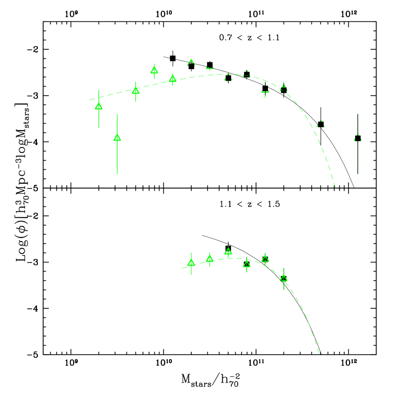
Figure 17: Effect of the correction for incompleteness on the Galaxy Stellar Mass Function in two redshift bins. Empty circles represent the GSMF computed on strictly mass–complete samples, while filled squares represent the GSMF computed on the “extended” sample with the correction for incompleteness applied, and solid line is the corresponding Schechter fit. Triangles show the GSMF computed on the “extended” sample without any correction for incompleteness, and dashed line the corresponding Schechter fit.

The practical effects of this correction are shown in Fig. 17, where we compare the GSMF with and without the applied correction, where we show that if we entirely ignore the incompleteness effects, the GSMF appears to drop significantly in the low mass bins.

References

- Baugh et al. (2002) Baugh, C., 2002 In: The Mass of Galaxies at Low and High Redshift. Proceedings of the ESO Workshop, Venice, Italy, 24-26 October 2001, p. 91.
- Bell et al. (2003) Bell, E.F., McIntosh, D. H., Katz, N., Weinberg, M.D., 2003, ApJS, 149, 289
- Bell et al. (2004) Bell, E.F., Wolf, C., Meisenheimer, K., et al., 2004, ApJ in press
- Bennet et al. (2003) Bennett, C.L., Halpern, M., Hinshaw, G., Karosik, N., et al., 2003, ApJS 148, 1
- (5) Benson, A.J., Frenk, C.S., & Sharples, R.M. 2002, ApJ, 574, 104
- (6) Bertin, E., & Arnouts, S. 1996, A&AS, 117, 393
- Brinchmann & Ellis (2000) Brinchmann,J. & Ellis R.S. 2000, ApJ 536L, 77B, BE00
- Broadhurst et al. (1992) Broadhurst, T.J. Ellis, R. S., Glazebrook, K., 1992, Nature 335, 55
- Bruzual & Charlot (2003) Bruzual, C. & Charlot, S. 2003, MNRAS, 344, 1000
- Calzetti et al. (2000) Calzetti, D. Armus, L. Bohlin, R.C., 2000, ApJ, 533, 682
- Cavaliere & Vittorini (2000) Cavaliere,A. & Vittorini,V., 2000, ApJ, 543, 599
- (12) Cen, R., Ostriker, J.P. 2000, 538, 83
- (13) Chapman, S. C.; Blain, A. W.; Ivison, R. J.; Smail, Ian R.; 2003, Nature, 422, 695
- (14) Cimatti A. Mignoli, M. Daddi, E., et al. 2002a, A&A, 392, 395 (Paper III)
- (15) Cimatti A., Pozzetti, L. Mignoli, M., et al. 2002b, A&A, 391L, 1 (Paper IV)
- (16) Cimatti A. Daddi, E. Mignoli, M., et al. 2002c, A&A, 381, L68 (Paper I)
- Cimatti et al. (2003) Cimatti A. et al. 2003, A&A 412L, 1
- Cohen et al. (1999) Cohen, J.G., Blandford, R. Hogg,D. W., ApJ, 512, 30
- Cohen (2002) Cohen, J., 2002, ApJ, 567, 672
- Cole et al. (2000) Cole, S., Lacey, C.G., Baugh, C.M., Frenk, C.S., et al., 2000, MNRAS, 319, 168
- Cole et al. (2001) Cole, S., Norberg, P., Baugh, C. M., et al., 2001, MNRAS, 326, 255
- (22) Daddi, E.; Cimatti, A.; Pozzetti, L.; Hoekstra, H.; Röttgering, H. J. A.; Renzini, A.; Zamorani, G.; Mannucci, 2000, A&A, 361, 535
- (23) Daddi, E.; Broadhurst, T.; Zamorani, G.; Cimatti, A.; Röttgering, H.; Renzini, A., 2001, A&A 376, 825
- Daddi et al (2002) Daddi, E., Cimatti, A., Broadhurst, T., et al. 2002, A&A, 384, L1 (Paper II)
- Daddi et al. (2004) Daddi,E. Cimatti,A., Renzini, A., et al. 2004a, ApJ, 600, L127
- (26) Daddi, E., et al., 2004b, A&A subm.
- (27) Dickinson, M. 2002, in The Mass of Galaxies at Low and High Redshift, ed. R. Bender & A. Renzini (Berlin: Springer), p. 324
- D (03) Dickinson, M., Papovich, C., Ferguson, H.C., Budavari, T., 2003, ApJ 587, 25, D03
- Drory et al. (2001) Drory, N., Bender, R., Snigula, J. , et al. 2001 ApJL, 562, 111
- Drory et al. (2001) Drory, N., Bender, R., et al. 2004 in press, astro-ph/0403041
- Evrard et al. (2002) Evrard, A.E., MacFarland,T.J., Couchman,H. M. P., et al., 2002, ApJ 573, 7
- (32) Ferrara, A., Bianchi, S., Cimatti, A., Giovanardi, C. 1999, ApJS, 123, 437
- Firth et al. (2002) Firth, A. E., Somerville, R. S., McMahon, R. G., et al., 2002, MNRAS, 332, 617
- Fontana et al. (1999) Fontana, A., Menci, N., D’Odorico, S., et al. MNRAS, 1999, ApJ, 310L, 27
- (35) Fontana, A.; D’Odorico, S.; Poli, F; Giallongo, E.; Arnouts, S.; Cristiani, S; Moorwood, A; Saracco, P. 2000, ApJ, 120, 2206
- F (03) Fontana, A., Donnarumma, I., Vanzella, E., et al., 2003, ApJ, 594L, 9, F03
- (37) Fukugita, M., Hogan, C.J., & Peebles, P.J.E. 1998, ApJ, 503, 518
- (38) Gao, L., Loeb A., Peebles, P. J. E., White, S. D. M., Jenkins, A. 2003, astro-ph/0312499
- Gavazzi et al. (1996) Gavazzi G., Pierini D., Boselli A. 1996, A&A, 312, 397
- (40) Geherels, 1986, ApJ, 303, 336
- Giallongo et al. (1998) Giallongo, E., D’Odorico, S., Fontana, A., 1998, AJ 115, 2169
- Gilli et al. (2003) Gilli, R. ,Cimatti, A., Daddi, E. et al., 2003 ApJ, 592, 721
- (43) Glazebrook et al., 2004, ApJ subm., astro-ph/0401037
- (44) Goldader, J. D.; Meurer, G; Heckman, T. M., et al, 2002, ApJ, 568, 651
- (45) Gould A; Bahcall, J. N.; & Flynn C.; 1996, ApJ, 465, 759
- (46) Granato, G.L.,Lacey, C. G.; Silva, L.; Bressan, A.; Baugh, C. M.; Cole, S.; Frenk, C. S.; 2000, ApJ, 542, 710
- (47) Granato, G.L.; Silva, L.; Monaco, P.; Panuzzo, P.; Salucci, P.; De Zotti, G.; Danese, L.2001, MNRAS, 324, 527
- (48) Granato, G.L.; De Zotti, G.; Silva, L.; Bressan, A.; Danese, L.; 2004 ApJ, 600, 580
- (49) Hernquist, X., & Springel, Y. 2003, MNRAS, 341, 1253
- Kauffmann et al. (1998) Kauffmann G., Charlot S. 1998, MNRAS, 297, L23
- Kauffmann et al. (2003) Kauffmann, G., Heckman, T. M., Tremoty, C. et al., 2003, MNRAS, 341, 33
- (52) Kennicutt, R., 1983, ApJ, 272, 54
- (53) Kroupa, P. 2001, MNRAS, 322, 231
- Lacey & Cole (1993) Lacey, C. & Cole, S, 1993, MNRAS, 262, 627
- (55) Lilly, S., S. J.; Le Fevre, O.; Crampton, David; Hammer, F.; Tresse, L. 1995, ApJ, 455, 50
- Madau et al. (1998) Madau P., Pozzetti L., Dickinson M., 1998, ApJ, 498, 106
- (57) Mathis, H.; Lemson, G.; Springel, V.; Kauffmann, G.; White, S. D. M.; Eldar, A.; Dekel, A., 2002, 2002, MNRAS, 333, 739
- Menci et al. (2002) Menci N., Cavaliere A., Fontana A., Giallongo E., Poli F.2002, ApJ, 575, 18
- Menci et al. (2004) Menci N.,Cavaliere A., Fontana A., Giallongo E.,Poli F., Vittorini V., 2004, ApJ in press, astro-ph/0311496
- Nagamine et al. (2001a) Nagamine, K. Fugugita, M. Cen, R., Ostriker, J.P. 2001a, MNRAS, 327L, 10
- (61) Nagamine, K. Fugugita, M. Cen, R., Ostriker, J.P. 2001b, ApJ, 558, 497
- (62) Nagamine, K., et al. 2004, ApJL subm, astro-ph/0311294
- Padmanabahn et al. (2003) Padmanabahn, N., Seljak, U., Strauss, M. A., et al. 2003, astro-ph/0307082
- Papovich et al. (2001) Papovich, C., Dickinson, M.M. Ferguson, H.C., 2001, ApJ, 559, 620
- (65) Persic, M., & Salucci, P. 1992, MNRAS, 258, 14p
- (66) Pettini, M. & Pagel, B.E.J., 2004, MNRAS, 348, 59
- Poli et al. (2001) Poli, F., Menci, N., Giallongo, E., et al., 2001, ApJ 551L, 45
- Poli et al. (2003) Poli, F., Giallongo, E., Fontana, A., et al., 2003, ApJL 593, 1
- (69) Postman, Marc; Lauer, Tod R.; Oegerle, William; Donahue, Megan, 2002, ApJ 579, 93
- Pozzetti et al. (1996) Pozzetti, L., Bruzual A., G., Zamorani, G. 1996, MNRAS, 281,953
- Pozzetti et al. (1998) Pozzetti, L., Madau P., Zamorani, G., Ferguson H.C., Bruzual,.G. 1998, MNRAS, 298, 1133
- Pozzetti et al. (2003) Pozzetti, L., Cimatti, A., Zamorani, G. et al., 2003, A&A 402 837 (Paper V)
- (73) Renzini, A. 1998, ASP Conf. Ser. 146, 298
- (74) Renzini, A. 1999a, in The Formation of Galactic Bulges, ed. C.M. Carollo et al. (Cambridge, CUP), 9
- (75) Renzini, A. 1999b, in Chemical Evolution from Zero to High redshift, ed. J.R. Walsh & M.R. Rosa (Berlin: Springer), p. 185
- (76) Renzini, A. 2003, in Clusters of galaxies: probes of Cosmological Structure and galaxy Evolution, ed. J.S. Mulchaey, A. Dressler, & A. Oemler (Cambridge: CUP), in press (astro-ph/0307146)
- (77) Rudnick, G., Rix, H.W., Franx, M. et al, 2003, ApJ, 599, 847
- Salpeter (1955) Salpeter, E. E., 1955, ApJ 121 , 161
- (79) Saracco, P.; Giallongo, E; Cristiani, S.; D’Odorico, S; et al. 2001, A&A 375, 1
- (80) Saracco, P. et al , 2004 A&A in press, (astro-ph/0310131)
- Shapley et al. (2001) Shapley, A. E., Steidel, C.C., Adelberger, K.L., et al, 2001, ApJ 562, 95
- (82) Somerville, R.S., Primack, J. R., 1999, MNRAS, 310, 1087
- (83) Somerville, R.S., Primack, J. R., Faber, S., 2001, MNRAS, 320, 504
- (84) Somerville et al. 2004a, in Multiwavelength Mapping of galaxy Formation and Evolution, ed. R. Bender & A. Renzini (Berlin: Springer), in press, astro-ph/0401570
- Somerville et al. (2004) Somerville, R. S., Moustakas, L. A., Baharam, M., et al., 2004b, ApJ, 600L, 135
- Songaila et al. (1994) Songaila, A., Cowie, L. L., Hu, E. M., Gardner, J. P., 1994, ApJS, 94, 416
- (87) Steidel, C. C., Adelberger, K. L., Giavalisco, M., Dickinson, M., & Pettini, M. 1999, ApJ, 519, 1
- (88) Zoccali, M., et al. 2000, ApJ, 530, 418