Full–Sphere Simulations of a Circulation–Dominated Solar Dynamo: Exploring the Parity Issue

^1,3Department of Physics, Indian Institute of Science, Bangalore-560012, India.
email: piyali@physics.iisc.ernet.in, arnab@physics.iisc .ernet.in
²Department of Physics, Montana State University, Bozeman, MT 59717, USA.
email: nandi@mithra.physics.montana.edu

Abstract

We explore a two-dimensional kinematic solar dynamo model in a full sphere, based on the helioseismically determined solar rotation profile and with an $\alpha$ effect concentrated near the solar surface, which captures the Babcock–Leighton idea that the poloidal field is created from the decay of tilted bipolar active regions. The meridional circulation, assumed to penetrate slightly below the tachocline, plays an important role. Some doubts have recently been raised regarding the ability of such a model to reproduce solar-like dipolar parity. We specifically address the parity issue and show that the dipolar mode is preferred when certain reasonable conditions are satisfied, the most important condition being the requirement that the poloidal field should diffuse efficiently to get coupled across the equator. Our model is shown to reproduce various aspects of observational data, including the phase relation between sunspots and the weak, diffuse field.

1 Introduction

Ever since Parker (1955) formulated the turbulent dynamo theory, varieties of very different dynamo models for the Sun have appeared in the literature. Within the last few years, however, a concensus view seems to be emerging as to what should be the basic characteristics of a solar dynamo model. The history of how this concensus view emerged is discussed in the Introduction of Nandy & Choudhuri (2001), with citations to important original papers. A more detailed account of the history can be found in the review by Choudhuri (2003a). We, therefore, begin here by summarizing the main aspects of this concensus view without getting into the details of history again.

One important ingredient of a solar dynamo model is the differential rotation, which has now been mapped by helioseismology. The toroidal magnetic field must be produced by the stretching of poloidal field lines primarily within the tachocline—the region of concentrated vertical shear at the base of the solar convection zone (SCZ). The toroidal field produced in the tachocline would then rise from there due to magnetic buoyancy to produce active regions. Simulations of flux rise through the SCZ suggested that the toroidal field at the bottom must be of order $10^{5}$ G (Choudhuri & Gilman 1987; Choudhuri 1989; D’Silva & Choudhuri 1993; Fan et al. 1993; D’Silva & Howard 1993; Caligari et al. 1995). Since such a strong field is expected to quench the usual mean field $\alpha$ effect (Parker 1955; Steenbeck et al. 1966), one possibility being considered by many researchers is that the poloidal field is generated at the surface from the decay of tilted bipolar region—an idea that goes back to Babcock (1961) and Leighton (1969). The poloidal component generated at the surface is first advected poleward by a meridional circulation (Wang et al. 1989a, 1989b; Dikpati & Choudhuri 1994, 1995; Choudhuri & Dikpati 1999). Finally, the poloidal component sinks with the downward flow at the poles and is brought to the tachocline where it can be stretched by the differential rotation to generate the toroidal field—thus completing the full cycle. Since advection by the meridional circulation plays such a crucial role in such a model, we would refer to this model as the circulation-dominated solar dynamo or CDSD model.

Although the above view of the solar dynamo arose by assimilating the ideas of many researchers over the years, Wang et al. (1991), Choudhuri et al. (1995) and Durney (1995, 1996, 1997) were amongst the first to demonstrate the crucial role which meridional circulation is expected to play in modern solar dynamo models. While Choudhuri et al. (1995) modeled the generation of poloidal field from the decay of active regions by introducing a phenomenological $\alpha$ parameter concentrated at the surface, Durney (1995, 1996, 1997) followed Leighton (1969) more closely to capture this effect by taking two flux rings of opposite polarity at the surface. Afterwards, Nandy & Choudhuri (2001) have demonstrated that these two approaches give qualitatively similar results. We shall develop our models by prescribing an $\alpha$ coefficient concentrated near the surface. Dikpati & Charbonneau (1999) and Küker et al. (2001) presented CDSD models with solar-like internal rotation and with such a specification of $\alpha$ effect. Since $\partial\Omega/\partial r$ has a larger amplitude at the high latitudes within the tachocline (where it is negative) rather than at low latitudes (where it is positive), solar-like rotation tends to produce strong toroidal fields at high latitudes, in apparent contradiction to the observed fact that sunspots always appear at low latitudes. Commenting on this problem, Dikpati & Charbonneau (1999) write: “this is an unavoidable inductive effect …and no change in model parameters can do away entirely with this feature”. Küker et al. (2001) point out: “All recent dynamo models with the observed rotation law are faced with this problem, even when the $\alpha$ effect has been strongly reduced in the polar region by the relation $\alpha\propto\sin^{2}\theta\cos\theta$, as we also did”.

Nandy & Choudhuri (2002) have recently shown in a brief communication that this problem can be solved by postulating a meridional flow penetrating somewhat deeper than hitherto believed. If the meridional flow goes below the tachocline near the poles, then the strong toroidal field produced within the tachocline at high latitudes is immediately pushed underneath into the convectively stable layers and cannot emerge at the high latitudes. The meridional flow then carries this toroidal field through the stable layers to low latitudes. There the meridional flow rises and the toroidal flux enters the SCZ to become buoyantly unstable and produce active regions at low latitudes. Such a penetrating meridional flow produces theoretical butterfly diagrams in remarkable agreement with the observed butterfly diagram. The conventional wisdom was that the toroidal field which forms sunspots at low latitudes must have been produced at the low latitude. With the helioseismically determined rotation profile, this seems unlikely and it may well be that the toroidal field is actually generated at the high latitude, even though it is not allowed to erupt there.

Recently it has been pointed out by Dikpati & Gilman (2001) and Bonanno et al. (2002) that the CDSD model with the Babcock–Leighton mechanism for producing the poloidal field near the surface may not give the magnetic configuration with the observed parity. Hale’s polarity law of bipolar sunspots suggests that the toroidal magnetic field is anti-symmetric across the solar equator, implying a dipolar parity. A majority of the CDSD models were solved within one hemisphere and the boundary conditions at the equator were taken such that the dipolar mode was forced. Dikpati and Gilman (2001) solved the dynamo problem in the full sphere and found that the CDSD model with the $\alpha$ effect concentrated near the top of the SCZ preferentially excites the quadrupolar mode in which the toroidal field is symmetric across the equator—opposite to what is observed. Only when the $\alpha$ effect was concentrated near the bottom of the SCZ, they found the dipolar parity in conformity with observations. Bonanno et al. (2002) confirmed these findings.

The aim of the present paper is to provide the technical details of our dynamo models not given in the earlier brief paper of Nandy & Choudhuri (2002), to check the parity of these dynamo models by extending our code from a hemisphere to a full sphere and to address some related issues. In the dipolar mode, the poloidal field lines have to connect across the equator. It is necessary for the poloidal field to diffuse efficiently for this to be possible. On the other hand, the diffusion of the toroidal field has to be suppressed if we want to ensure that the toroidal field has opposite signs on the two sides of the equator. Since the toroidal component is much stronger than the poloidal component, we expect the turbulent diffusion to be much less effective on the toroidal component than on the poloidal component. On using a high diffusivity for the poloidal field and a low diffusivity for the toroidal field, we find that the dipolar parity is preferred. There is no need to include an additional $\alpha$ effect at the bottom of SCZ to ensure dipolar parity.

Since the nature of the meridional circulation plays such a crucial role in our model, let us make a few comments on it. Within the last few years, helioseismic techniques have given us some information about the sub-surface meridional circulation to a depth of about 15% of the solar radius (Giles et al. 1997; Braun & Fan 1999). So far there is no convincing observational evidence for an equatorward counter-flow deeper down, though it must exist to conserve mass. It is generally believed that the turbulent stresses in the SCZ drive the meridional circulation, although the details of how this happens are not understood (see, for example, Gilman 1986, §3.4.2). So the meridional circulation is expected to be confined to the convection zone. However, it is conceivable that an equatorward meridional transport of material takes place in the overshoot layer below the bottom of SCZ. This view is supported by recent simulations of solar convection (Miesch et al. 2000). A dynamo model with a meridional flow through the convectively stable overshoot layer seems, at the present time, to be the model with minimal extraneous assumptions which gives satisfactory results.

In the next section, we describe the basic features of our model. Then §3 focuses on the parity question and discusses the conditions to be satisfied to ensure the correct parity. In §4 we present some more details of what we consider our standard solar dynamo model, along with comparisons with observations. Finally our conclusions are summarized in §6.

2 Mathematical Formulation

2.1 The basic equations and boundary conditions

All our calculations are done with a code for solving the axisymmetric kinematic dynamo problem. An axisymmetric magnetic field can be represented in the form

$${\bf B}=B(r,\theta){\bf e}_{\phi}+\nabla\times[A(r,\theta){\bf e}_{\phi}],$$ (1)

where $B(r,\theta)$ and $A(r,\theta)$ respectively correspond to the toroidal and poloidal components. The standard equations for the so-called $\alpha\omega$ dynamo problem are:

$$\frac{\partial A}{\partial t}+\frac{1}{s}({\bf v}.\nabla)(sA)=\eta_{p}\left(\nabla^{2}-\frac{1}{s^{2}}\right)A+\alpha B,$$ (2)

$$\frac{\partial B}{\partial t}+\frac{1}{r}\left[\frac{\partial}{\partial r}(rv_{r}B)+\frac{\partial}{\partial\theta}(v_{\theta}B)\right]=\eta_{t}\left(\nabla^{2}-\frac{1}{s^{2}}\right)B+s({\bf B}_{p}.\nabla)\Omega+\frac{1}{r}\frac{d\eta_{t}}{dr}\frac{\partial{B}}{\partial{r}}$$ (3)

where $s=r\sin\theta$. Here ${\bf v}$ is the meridional flow, $\Omega$ is the internal angular velocity of the Sun and $\alpha$ is the coefficient which describes the generation of poloidal field at the solar surface from the decay of bipolar sunspots. We allow the turbulent diffusivities $\eta_{p}$ and $\eta_{t}$ for the poloidal and toroidal components to be different. We describe below how we specify ${\bf v}$, $\Omega$, $\eta_{p}$, $\eta_{t}$, and $\alpha$. Once these quantities are specified, we can solve (2) and (3) to study the behaviour of the dynamo. Apart from the specification of these parameters, we also include magnetic buoyancy in a way described below. We carry out our calculations in a meridional slab $R_{b}=0.55R_{\odot}<r<R_{\odot}$, $0<\theta<\pi$.

The boundary conditions are as follows. At the poles ($\theta=0,\pi$) we have

$$A=0,\ B=0.$$ (4)

For a perfectly conducting solar core, the bottom boundary ($r=R_{b}$) condition should be

$$A=0,\ B=0.$$ (5)

However, if the bottom of the integration region is taken well below the depths to which the meridional circulation reaches (and hence below the depths to which magnetic fields are carried), then the solutions are rather insensitive to the bottom boundary condition. We carried out some calculations by changing the bottom boundary condition of the toroidal field from $B=0$ to

$$\frac{\partial}{\partial r}(rB)=0.$$ (6)

The solutions remained virtually unchanged. At the top ($r=R_{\odot}$), the toroidal field has to be zero ($B=0$) and $A$ has to match smoothly to a potential field satisfying the free space equation

$$\left(\nabla^{2}-\frac{1}{r^{2}\sin^{2}\theta}\right)A=0.$$ (7)

Dikpati and Choudhuri (1994) describe how this is done.

We have used a finer grid resolution as compared to other models existing in the literature, with $129\times 129$ grid cells in the latitudinal and radial directions. The algorithm used by us in developing the numerical code is described in the Appendix of Dikpati & Choudhuri (1994) and the Appendix of Choudhuri & Konar (2002). If either the $\alpha$ coefficient has a quenching factor or magnetic buoyancy is included to suppress the growth of the magnetic field, then any arbitrary initial condition either asymptotically goes to zero (sub-critical condition) or relaxes to a steady dynamo solution (super-critical condition). We now discuss how the various parameters are specified.

2.2 Internal rotation $\Omega$

We use the following analytic form to represent the solar internal rotation (Schou et al. 1998; Charbonneau et al. 1999):

$$\Omega(r,\theta)=\Omega_{RZ}+\frac{1}{2}\left[1+\mbox{erf}\left(2\frac{r-r_{t}}{d_{t}}\right)\right]\left[\Omega_{SCZ}(\theta)-\Omega_{RZ}\right].$$ (8)

This analytical expression fits the results of helioseismology fairly closely for the following values of parameters: $r_{t}=0.7R_{\odot}$, $d_{t}=0.05R_{\odot}$ $\Omega_{RZ}/2\pi=432.8$ nHz, $\Omega_{SCZ}(\theta)=\Omega_{EQ}+\alpha_{2}cos^{2}(\theta)+\alpha_{4}cos^{4}(\theta)$, with $\Omega_{EQ}/2\pi=460.7$ nHz, $\alpha_{2}/2\pi=-62.69$ nHz and $\alpha_{4}/2\pi=-67.13$ nHz. A contour plot of $\Omega$ generated by the above expression is shown in Fig. 2, in which the tachocline is shown as a shaded region. Since helioseismology has already determined $\Omega$, we do not have much freedom to vary its parameters. At the present time, however, there exist some uncertainties as to the exact location of the tachocline and its thickness. These are indicated by the parameters $r_{t}$ and $d_{t}$. Especially, it is still not completely clear how the tachocline is located with respect to the bottom of the convection zone (whether it is completely below the convection zone or partly inside it). There are some indications that the tachocline may actually have a prolate shape, such that more of the tachocline comes within the convection zone at higher latitudes than at the lower latitudes. Given the many other uncertainties in the problem, we have not taken this effect into account in our calculations.

We take the bottom of the convection zone at $r=0.71R_{\odot}$, which is marked in Fig. 2. By bottom of the convection zone, we mean the depth at which the temperature gradient changes from being sub-adiabatic below to super-adiabatic above. As we point out later, magnetic buoyancy is assumed to be operative only above the bottom of the convection zone. Since the strong toroidal field is generated in the tachocline, a tachocline below the convection zone would imply a situation where the toroidal field is created at a location which is immune to magnetic buoyancy. Hence, the location of the tachocline with respect to the base of the convection zone is of considerable importance in our problem. As seen in Fig. 2, we take part of the tachocline above the bottom of the convection zone. All our calculations are done with this assumed profile of $\Omega$.

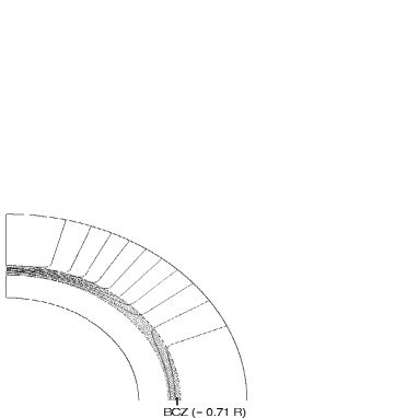
Figure 1: Contours of constant angular velocity as obtained from (8) and used in all of our calculations. The tachocline is indicated as the shaded region. The bottom of the convection zone (BCZ) is at 0.71R_⊙. The differential rotation being symmetric about the equator, only one quadrant is shown.

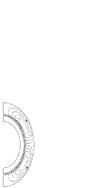
Figure 2: Streamlines of meridional circulation obtained by taking penetration radius $R_{p}=0.61R_{\odot}$. The tachocline is shown as a shaded region. Arrows denote the direction of flow.

In some of our earlier work (Choudhuri et al. 1995; Nandy & Choudhuri 2001; Nandy 2002), we had taken $\Omega$ to be independent of $\theta$ and used a radial variation appropriate for the equatorial region. If $\Omega$ is taken to be a function of $r$ alone, then the behaviour of the dynamo is much simpler. On the other hand, when $\Omega$ is a function of both $r$ and $\theta$ as given by (8), the problem becomes immensely more complicated.

2.3 Meridional circulation v

We now describe how the meridional circulation is specified in the northern hemisphere. The circulation in the southern hemisphere is simply obtained by a mirror reflection of the velocity field across the equator. We get the meridional circulation from the stream function $\psi$ defined through the equation

$$\rho{\bf v}=\nabla\times[\psi(r,\theta){\bf e}_{\phi}].$$ (9)

Assuming a density stratification

$$\rho=C\left(\frac{R_{\odot}}{r}-\gamma\right)^{m},$$ (10)

we take

$$\psi r\sin\theta=\psi_{0}(r-R_{p})\sin\left[\frac{\pi(r-R_{p})}{(R_{\odot}-R_{p})}\right]\{1-e^{-\beta_{1}r\theta^{\epsilon}}\}\{1-e^{\beta_{2}r(\theta-\pi/2)}\}e^{-((r-r_{0})/\Gamma)^{2}}$$ (11)

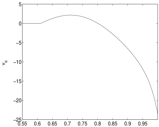
Figure 3: Plot of $v_{\theta}$ (in m s^-1) as a function of $r$ at the mid-latitude $\theta=45^{\circ}$.

with the following values of the parameters: $\beta_{1}=1.36\times 10^{-8}$ m^-1, $\beta_{2}=1.63\times 10^{-8}$ m^-1, $\epsilon=2.0000001$, $r_{0}=(R_{\odot}-R_{b})/4.0$, $\Gamma=3.47\times 10^{8}$ m, $\gamma=0.95$, $m=3/2$. It is the parameter $R_{p}$ which determines the depth to which the meridional circulation penetrates. Fig. 2 shows the streamlines of the meridional circulation obtained by taking $R_{p}=0.61R_{\odot}$, which is used in all our calculations and which corresponds to the meridional flow going slightly below the tachocline. The amplitude of the meridional circulation is fixed by $\psi_{0}/C$. We choose it such that the poleward flow near the surface at mid-latitudes peaks typically around $v_{0}=22$ m s^-1. The equatorward counterflow peaks at the core-convection zone interface and has a value of 1.8 m s^-1, which is similar to what observational analysis of sunspot drift suggests (Hathaway et al. 2003). Since the form of the meridional circulation seems crucial for the stability for the dynamo, let us make some comments on it. On comparing (11) with equation (9) of Nandy & Choudhuri (2001), it will be found that we have now added an extra factor $(r-R_{p})$ just after $\psi_{0}$. This extra factor ensures that $v_{\theta}$ smoothly falls to zero at $R_{p}$. If this factor is not included, then $v_{\theta}$ has a finite value at $R_{p}$, leading to a discontinuity at $R_{p}$ if there is no flow below. Fig. 3 shows the profile of $v_{\theta}$ at the mid-latitude obtained with the factor $(r-R_{p})$ included. It should also be noted in Fig. 3 that $v_{\theta}$ in our model decreases monotonically below the bottom of the SCZ and becomes very small in the tachocline. We want to emphasize that we need very modest flows below the tachocline (presumably not much beyond the region of overshooting) to make our model work.

We point out that we find well-behaved periodic solutions only for certain forms of the meridional circulation. Küker et al. (2001) also found oscillatory solutions only within limited regions of parameter space. However, the dynamo becomes very robust and stable with a sufficiently deeply penetrating meridional flow having a smooth $v_{\theta}$ profile.

2.4 Diffusion coefficients $\eta_{p}$ and $\eta_{t}$

We expect the turbulent diffusivity inside the convection zone $\eta_{SCZ}$ to be much larger than the diffusivity $\eta_{RZ}$ in the radiative interior, the overshoot layer being the region within which the value of diffusivity makes a transition from $\eta_{RZ}$ to $\eta_{SCZ}$. Since the poloidal component is weak, the turbulent diffusivity acts on it without any difficulty. We take the diffusivity for the poloidal component to be

$$\eta_{p}(r)=\eta_{RZ}+\frac{\eta_{SCZ}}{2}\left[1+\mbox{erf}\left(\frac{r-r_{BCZ}}{d_{t}}\right)\right]$$ (12)

Fig.5 shows a plot of $\eta_{p}$ with the following values of the parameters: $\eta_{SCZ}=2.4\times 10^{12}$cm² s^-1, $\eta_{RZ}=2.2\times 10^{8}$ cm² s^-1, $r_{BCZ}=0.7R_{\odot}$, $d_{t}=0.05R_{\odot}$.

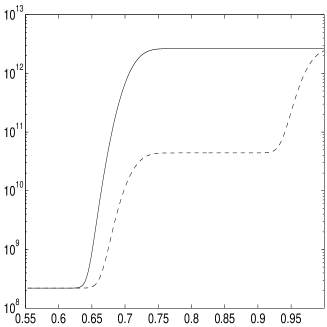
Figure 4: Plots of $\eta_{p}(r)$(solid) and $\eta_{t}(r)$ (dashed) as given by (12) and (13) as functions of the fractional radial distance ($r/R_{\odot}$). y-axis is in units of cm² s^-1.

Figure 5: Plots of $\eta_{p}(r)$(solid) and $\eta_{t}(r)$ (dashed) in cm² s^-1 used in §3.2, as function of the fractional radial distance ($r/R_{\odot}$).

The toroidal component, however, has a value larger than the equipartition value till it rises to about 30,000 km or 40,000 km below the solar surface (Longcope & Choudhuri 2002, §2). Only in the top layers of the SCZ, the diffusion coefficient of the toroidal component should be equal to the usual turbulent diffusivity value $\eta_{SCZ}$. Within the main body of SCZ, the action of turbulent diffusivity on the toroidal component must be considerably suppressed. In view of this, we take the diffusivity $\eta_{t}$ of the toroidal component as shown in Fig. 5, which is generated from the expression

$$\eta_{t}(r)=\eta_{RZ}+\frac{\eta_{SCZ1}}{2}\left[1+\mbox{erf}\left(\frac{r-r^{\prime}_{BCZ}}{d_{t}}\right)\right]+\frac{\eta_{SCZ}}{2}\left[1+\mbox{erf}\left(\frac{r-r_{TCZ}}{d_{t}}\right)\right]$$ (13)

with $\eta_{SCZ}=4\times 10^{10}$cm² s^-1, $r^{\prime}_{BCZ}=0.72R_{\odot}$ and $r_{TCZ}=0.95R_{\odot}$. As we shall see below, $\eta_{p}$ and $\eta_{t}$ specified in this way gives solutions with dipolar parity. Except §3.2–3, everywhere else in our paper we use $\eta_{p}$ and $\eta_{t}$ as specified above.

Simulations of the evolution of the weak, diffuse field on the solar surface (Wang et al. 1989a,b), as well as observational estimates from sunspot decay, point out that $\eta_{SCZ}$ must be of the order of $10^{12}$ cm² s^-1 in the upper layers of the convection zone. We have taken a value of this order on the higher side and find that it allows sufficient diffusion of the poloidal component across the equator to enforce the dipolar mode. A low value of diffusivity below the bottom of the convection zone is very important in dynamo models with meridional flow penetrating below the tachocline. A low diffusivity in the tachocline and the overshoot layer ensures that the toroidal field which is produced in the high latitudes within the tachocline does not decay much while being transported to low latitudes by the meridional flow (Nandy 2002). The assumed value of $\eta_{RZ}$ essentially ensures that the magnetic field is frozen for time scales of the order of dynamo period. By taking a low $\eta_{t}$ at the bottom of SCZ, we also make sure that there is not much cross-diffusion of the toroidal component across the equator and it is possible for the toroidal component to have opposite values in the two hemispheres. It may be noted that there is a term involving $d\eta_{t}/dr$ in the evolution equation (3) for the toroidal component. This term has the form of an advection term, with $d\eta_{t}/dr$ corresponding to a downward velocity. We discovered an error in the original code which produced the results of Nandy & Choudhuri (2002). The error made this term involving $d\eta_{t}/dr$ somewhat smaller than what it should have been. However, on incorporating the suppression of $\eta_{t}$ in the body of the SCZ as we do here, the gradient $d\eta_{t}/dr$ is moved to the upper layers (which can be seen from Fig. 5) and the results essentially remain the same as earlier.

For the sake of comparison, we present in §3.2–3 some results obtained with a lower diffusivity for the poloidal field. The profile of this $\eta$ is shown in Fig. 5. This low diffusivity does not allow the poloidal components in the two hemispheres to connect across the equator and usually the quadrupolar mode is preferred, as we shall see in §3.2–3.

2.5 The $\alpha$ coefficient

The $\alpha$ coefficient is taken in the form

$$\alpha=\alpha_{0}\cos\theta\frac{1}{4}\left[1+\mbox{erf}\left(\frac{r-r_{1}}{d_{1}}\right)\right]\times\left[1-\mbox{erf}\left(\frac{r-r_{2}}{d_{2}}\right)\right].$$ (14)

The parameters we use are $r_{1}=0.95R_{\odot}$, $r_{2}=R_{\odot}$, $d_{1}=d_{2}=0.025R_{\odot}$, making sure that the $\alpha$ effect is concentrated in the top layer $0.95R_{\odot}\leq r\leq R_{\odot}$. The solid line in Fig. 6 shows the variation of $\alpha$ with $r$. The amplitude $\alpha_{0}$ is taken such that the dynamo is super-critical. We had taken $\alpha_{0}=$ 25 m s^-1 in most of our calculations, where the solutions are found to be super-critical for such a value of $\alpha_{0}$. We use this form of $\alpha$ coefficient in all our calculations except in §3.3, where an additional $\alpha$ effect within the SCZ is included. The dashed line in Fig. 6 shows the radial profile of $\alpha$ used in §3.3, the angular variation being taken as $\cos\theta$ as used elsewhere in the paper.

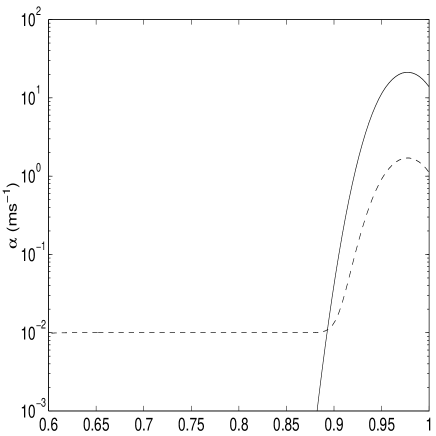
Figure 6: The Babcock-Leighton $\alpha$ used for most of our calculations (solid line) and also in our standard model described in §3.1. The dashed line shows the $\alpha$ used in §3.3, as a function of fractional radial distance $r/R_{\odot}$. Units are in m s^-1.

It should be noted that $\alpha$ coefficient in a Babcock–Leighton dynamo is not given by the mean helicity of turbulence as in mean field MHD (see, for example, Choudhuri 1998, §16.5). In our approach as well in the approach of several other authors (Choudhuri et al. 1995; Dikpati & Charbonneau 1999; Nandy & Choudhuri 2001; Küker et al. 2001), the $\alpha$ coefficient phenomenologically captures the effect of poloidal field generation from the decay of tilted active regions near the solar surface. The angular factor $\cos\theta$ arises from the angular dependence of the Coriolis force which causes the tilts of active regions. Several groups suppressed $\alpha$ artifically at high latitudes to reduce the strength of the toroidal field at high latitudes. Dikpati & Charbonneau (1999) used the angular factor $\cos\theta\sin\theta$, whereas Küker et al. (2001) used $\cos\theta\sin^{2}\theta$. Flux tube simulations which calculate the tilts of emerging active regions (D’Silva & Choudhuri 1993; Fan et el. 1993) give us some clues about the angular dependence of the $\alpha$ coefficient. If the Coriolis force could freely produce the tilt without any opposing force operative, then the tilts at different latitudes would have been proportional to the Coriolis factor $\cos\theta$ and the $\alpha$ coefficient would have the same angular dependence. However, the Coriolis force is opposed by magnetic tension which tries to prevent the tilt from becoming very large. We thus find that the tilt does not increase with latitude as fast as the Coriolis factor $\cos\theta$. On these grounds, we expect that $\alpha$ will not increase with latitude as fast as $\cos\theta$, but taking the angular dependence to be $\cos\theta\sin\theta$ or $\cos\theta\sin^{2}\theta$ may be unrealistic.

We also point out that we have eliminated the $\alpha$-quenching factor typically taken to be of the form $(1+B^{2}/B_{0}^{2})^{-1}$. If magnetic buoyancy is not included, then such a factor is the only source of nonlinearity in the model and is essential to allow the simulation to relax to steady solutions. We found the $\alpha$-quenching to be redundant in presence of magnetic buoyancy which limits the toroidal field to values $<10^{5}$ G (see §2.5). On theoretical grounds also, the removal of $\alpha$-quenching is quite logical in the Babcock–Leighton dynamo models. In mean field MHD, the $\alpha$ effect comes from helical turbulence which is quenched when the magnetic field is super-equipartition. In our model, however, the $\alpha$ effect is due to the decay of tilted bipolar regions. Flux tube simulations do show that the tilt is less for stronger magnetic fields at the bottom of the SCZ (see D’Silva & Choudhuri 1993). So the $\alpha$ effect should depend on the magnetic field at the bottom of SCZ, but not on the local value of the magnetic field at the surface where the $\alpha$ effect is operative. Since our formulation of magnetic buoyancy (see §2.6) makes the toroidal field erupt only when it is of order $10^{5}$ G, we do not expect much variation in $\alpha$ with the magnetic field.

2.6 Magnetic buoyancy

We prescribe magnetic buoyancy in a way which has been discussed in detail by Nandy & Choudhuri (2001) and Nandy (2003). We search for toroidal field $B$ exceeding the critical field $B_{c}=10^{5}$ G, above the base of the SCZ taken at $r=0.71$ at intervals of time $\tau=8.8\times 10^{5}$ s. Wherever $B$ exceeds $B_{c}$, a fraction $f=0.5$ of it is made to erupt to the surface layers, with the toroidal field values adjusted appropriately to ensure flux conservation. The parameter $f$ measures the strength of magnetic buoyancy. It was found by Nandy & Choudhuri (2001) that, when $f$ was still small compared to 1 ($f$ has to be less than 1), magnetic buoyancy already reached saturation and the character of the dynamo did not change any more on increasing $f$. The value $f=0.5$ used throughout our paper already puts the dynamo in the buoyancy-saturated regime.

Although $A$ and $B$ in general evolve according to (2) and (3), we allow abrupt changes in $B$ after intervals of $\tau$ to take account of magnetic buoyancy. While our treatment of magnetic buoyancy may not be fully satisfactory, note that uncertainties remain in the way buoyancy has been handled earlier by other groups, e.g. by treating buoyancy as a simple loss term (Schmitt & Schüssler 1989) or by treating it in a non-local manner by making the poloidal source term near the surface proportional to the toroidal field strength at the bottom of the SCZ (Dikpati & Charbonneau 1999).

3 The parity question

All our calculations are done with internal rotation $\Omega$, meridional circulation ${\bf v}$ and magnetic buoyancy as specified in §2.2, §2.3 and §2.6. We first present results in §3.1 obtained with the diffusion coefficients shown in Fig. 5 and an $\alpha$ effect concentrated near the surface as shown in Fig. 6 by the solid line. The dipolar mode is the clearly preferred mode and the results qualitatively match the observational data quite well. Some authors (Dikpati & Gilman 2001; Bonanno et al. 2002) obtained anti-solar quadrupolar modes in their calculations. We believe that this was due to the low diffusivity of the poloidal component which did not allow this component to connect across the equator. We present results in §3.2 in which the diffusion coefficients are as shown in Fig. 5, i.e. the diffusivity of the poloidal component is reduced compared to what we use in §3.1 and that of the toroidal field is increased. We end up with the anti-solar quadrupolar parity in this case. Then we show in §3.3 that we get back the dipolar parity if we include an $\alpha$ effect within the SCZ (as shown by dashed line in Fig. 6), while keeping all the other things the same as in §3.2. This is again in agreement with what Dikpati & Gilman (2001) and Bonanno et al. (2002) found. We are thus able to reproduce the results of Dikpati & Gilman (2001) and Bonanno et al. (2002). However, we do not agree with their conclusion that a pure Babcock-Leighton $\alpha$ effect concentrated near the solar surface cannot give the dipolar parity. As we show in §3.1, the dipolar parity is the preferred parity if the diffusivity of the poloidal component is sufficiently high, even when the $\alpha$ effect is concentrated near the solar surface.

3.1 Solution with dipolar parity

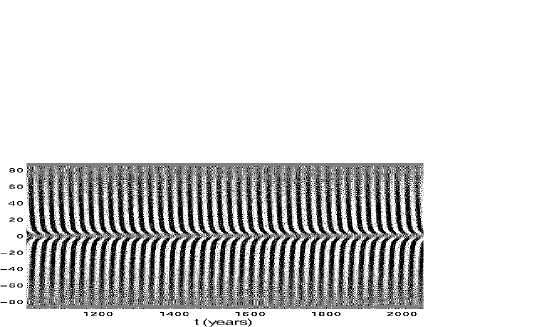
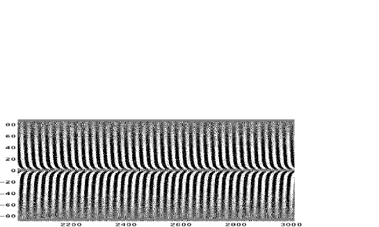
Figure 7: A time-latitude plot showing the evolution of the toroidal field at the bottom of the convection zone ($r$ = 0.71 $R_{\odot}$) starting from an initial quadrupolar (anti-solar) mode to a pure dipolar (solar-like) mode taking a duration of 3000 years, for the case presented in §3.1. The upper panel shows the evolution from 1000 - 2000 years whereas the lower panel traces the last thousand years (2000 - 3000 years). Regions shaded in white show positive $B$, whereas black regions denote negative $B$.

We first present a purely Babcock–Leighton dynamo ($\alpha$ effect concentrated near the surface as shown in Fig. 6 by solid line), which settles into dipolar parity. As we discussed above, the preferred parity depends on the diffusion coefficients. Various experiments with the parameter space of the model tell us that there are two important conditions for getting the right parity.

1. The term $\eta_{RZ}$ representing the molecular diffusivity in the overshoot layer and the radiation zone below must be sufficiently small($\sim$ 2.2$\times$ 10⁸ cm² s^-1) to prevent the toroidal field from diffusing across the equator.

2. The diffusivity of the poloidal field $\eta_{p}$ within the SCZ must be sufficiently large ($\sim$ 2.4 $\times$ 10¹² cm² s^-1) to allow diffusive coupling of the poloidal field between two hemispheres.

Further, we have to avoid a large gradient $d\eta_{t}/dr$ at the bottom of the SCZ in order to obtain well-behaved solutions.

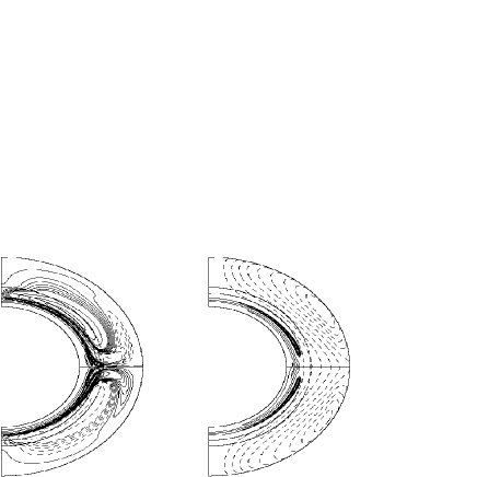
Figure 8: A snapshot of (a) the contours of toroidal field $B$ and (b) streamlines of the poloidal field, given by contours of constant $A$sin$\theta$, for the case of dipolar parity solution presented in §3.1. The solid lines denote positive $B$ or $A$, whereas dashed lines denote negative $B$ or $A$.

The particular solution we present here is obtained with the diffusion coefficients as given in Fig. 5. To ensure that the dipolar parity is the dominant mode in the model, we start from a pure quadrupolar initial condition and find that the solution eventually relaxes to a pure dipolar parity. Fig. 7 shows the evolution of the initial quadrupolar field into a dipolar field within a duration of 3000 years. Fig. 8 gives a snapshot of the relaxed magnetic field configuration, showing that the poloidal field lines have connected across the equator, whereas the toroidal field within the tachocline has opposite signs on the two sides of the equator. We carried out the simulation for another 3000 years after the solution relaxed to the dipolar mode, and the solution remained in the solar-like parity state during the entire run. We shall provide further details of this solution in §4.

3.2 Solution with quadrupolar parity

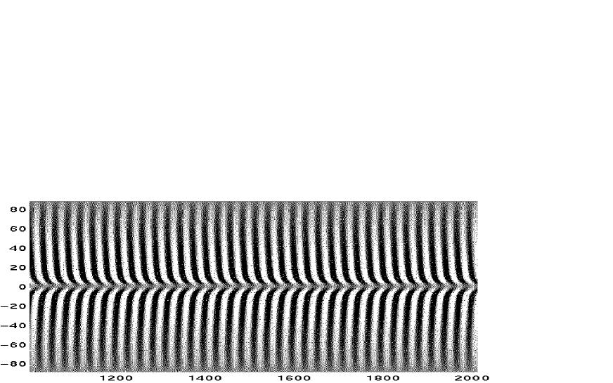
Figure 9: Time-latitude plot showing the evolution of $B$ at the bottom of the convection zone from an initial dipolar state to the preferred quadrupolar state, taking a duration of 2000 years, for the case presented in §3.2. Only the last 1000 years of model run is shown.

We now present a solution obtained by keeping all the parameters the same as in §3.1, except that we change the diffusion coefficients to what is shown in Fig. 5 rather than what is shown in Fig. 5 (as used in §3.1). The lower diffusivity of the poloidal field does not allow it to connect across the equator and we find that the quadrupolar mode is preferred. To make sure that indeed the dominant mode in this case is the quadrupolar mode, we started with an initial condition having dipolar parity and found that it relaxed to a quadrupolar parity. Fig. 9 presents a theoretical butterfly diagram showing this transition process, whereas Fig. 10 illustrates the magnetic field configuration after the dynamo has settled into a quadrupolar mode. We find that the poloidal field has not diffused enough to connect across the equator, but has remained separated on the two sides of the equator. On the other hand, the toroidal field in the tachocline has the same sign on the two sides of the equator and makes up a patch of a common sign across the equator. We have made many runs for other values of diffusion coefficients. As we already mentioned, a low diffusivity $\eta_{RZ}$ below the bottom of the SCZ is an essential requirement to obtain the dipolar parity (to ensure that the toroidal field in the tachocline cannot diffuse much across the equator). When we take $\eta_{RZ}$ larger than about $2\times 10^{9}$ cm² s^-1, we found that we always got quadrupolar solutions and it was not possible to get dipolar solutions even by increasing $\eta_{p}$ in the SCZ to facilitate the coupling of the poloidal field across the equator. We have shown in Fig. 9 a transition from a dipolar parity to a quadrupolar parity in a case in which the quadrupolar parity is preferred. How fast such a transition takes place depends on the value of $\eta_{RZ}$. On using $\eta_{RZ}\sim 2\times 10^{10}$ cm² s^-1, the change-over takes place within just 300 years, whereas decreasing $\eta_{RZ}$ by two orders of magnitude stretches the time scale of transition to the quadrupolar parity to 2000 years.

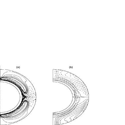
Figure 10: A snapshot of (a) the contours of the toroidal field and (b) streamlines of the poloidal field, for the quadrupolar parity solution presented in §3.2.

3.3 Solution with $\alpha$ effect inside the SCZ

Finally we consider what influence an additional $\alpha$ effect within the SCZ has on the parity of the solution. For this purpose, we change the radial profile of the $\alpha$ effect to what is shown in Fig. 6 by a dashed line rather than the solid line in the same figure, keeping the other things the same as in §3.2 (including the diffusion coefficients which are as shown in Fig. 5). We find that the solution relaxes to dipolar parity even if we start from quadrupolar parity, as shown in Fig. 11. A snapshot of the field configuration is presented in Fig. 12. This is a case in which the quadrupolar parity would have been preferred if the additional $\alpha$ effect inside the SCZ were not present, as we saw in §3.2. However, this additional $\alpha$ effect, even though its value inside the SCZ is much smaller than the value of the Babcock–Leighton $\alpha$ at the surface, can make the solution dipolar. This is in agreement with what has been found by Dikpati & Gilman (2001) and Bonanno et al. (2002). One has to keep in mind that the $\alpha$ coefficient has to be multiplied by the toroidal field B to provide the source term for the poloidal field. Since B is very large at the bottom of the SCZ, even a very small $\alpha$ there can make $\alpha B$ as large as what it is near the surface. That is why we find that even a very small $\alpha$ inside the SCZ or at its base can affect the nature of the solution so drastically. Presumably, an $\alpha$ effect within the SCZ creates some poloidal field there which can diffuse across the equator more efficiently than poloidal field created near the surface, thereby enforcing the dipolar parity. Note that in the presence of a small $\alpha$ inside the SCZ the magnitude of the Babcock-Leighton $\alpha$ required at the surface for steady oscillating solutions decreases by almost a factor of 10 (dashed line in Fig.6).

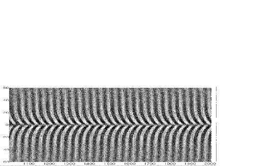
Figure 11: Time-latitude plot showing the evolution of the toroidal field $B$ at the bottom of the convection zone, with an additional $\alpha$ introduced inside the SCZ, as presented in §3.3. Last 1000 years of the 2000 year long model run is shown.

Choudhuri (2003b) has argued that the strong toroidal field at the bottom of the SCZ would be highly intermittent and the $\alpha$ effect may be operative in the intervening regions of weak field. Several other authors (Ferriz-Mas et al. 1994; Dikpati & Gilman 2001) argue that the various instabilities associated with the strong field also can produce something like an $\alpha$ effect. So an additional $\alpha$ effect within the SCZ or at its bottom is certainly a realistic possibility. However, our knowledge about it at the present time is very incomplete and uncertain. On the other hand, we see tilted active regions decay on the solar surface and we directly know from observations that there is an $\alpha$ effect at the solar surface. By the Occam’s razor argument, we feel that it is desirable to first construct solar dynamo models with this Babcock–Leighton $\alpha$ alone—especially since we have shown in §3.1 that it is possible to get solar-like dipolar parity with such dynamo models. We present a more detailed discussion of such pure Babcock–Leighton dynamo models in §4.

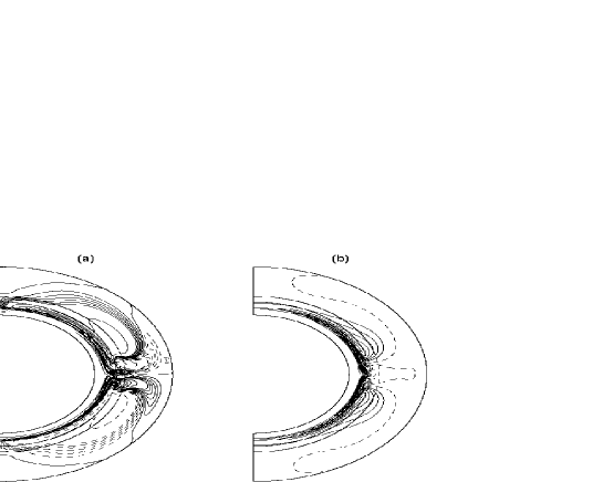
Figure 12: A snapshots of (a) the toroidal field contours and (b) streamlines of the poloidal field, for the solution presented in §3.3.

4 Towards a Standard Model

We have seen in §3.1 that a CDSD model with an $\alpha$ effect concentrated near the surface and with appropriate values of various parameters can give a solution with the dipolar parity. We would refer to this solution as our standard model. We have focused primarily on the parity of this solution in §3.1. Now we discuss other aspects of this solution and show that this solution matches observational data quite well. We have already discussed in §2 and §3.1 how the various parameters of this particular case are specified. The amplitude of the Babcock-Leighton $\alpha$ effect used to generate our standard solution is 25 m s^-1. For this standard case, we refined our grid to have 257$\times$257 points, and the results remained unchanged with this finer resolution.

Fig. 13 shows the time-latitude contour plot of the radial field at the solar surface, with the theoretical butterfly diagram superimposed upon it. The butterfly diagram is producing by marking the locations of eruption, ‘+’ indicating the positive value of $B$ at the bottom of the SCZ which erupts and ‘o’ indicating the negative value. The sunspot eruptions are confined within $\pm$ 40^o and the butterfly diagrams have shapes similar to what is observationally found (see, for example, Fig. 6.2 in Choudhuri 2003a; Hathaway et al. 2003). The weak radial field migrates poleward at higher latitudes, in conformity with observations. One of the important aspects of observational data is the phase relation between the sunspots and the weak diffuse field. See §1 of Choudhuri & Dikpati (1999) for a detailed discussion of this (especially note Fig. 1 there). The polar field changes from positive to negative at the time of a sunspot maximum corresponding to a negative toroidal field $B$ at the base of SCZ. This is clearly seen in the theoretical results shown in Fig. 13. In Fig.14 we show four snapshots of the toroidal field contours and poloidal field lines taken successively at an interval of $1/8^{\rm{th}}$ the solar cycle period which happens to be about 25 years in this case. In all the snapshots we see that the poloidal field lines are symmetric about the equator. The $\eta_{p}$ in the convection zone is sufficiently high ($\sim 2.4\times 10^{12}$ cm² s^-1) to ensure that the poloidal fields connect smoothly across the equator. On the other hand, the toroidal fields on the two sides of the equator, which have opposite signs, cannot diffuse together due to the low $\eta_{t}$ near the base of SCZ.

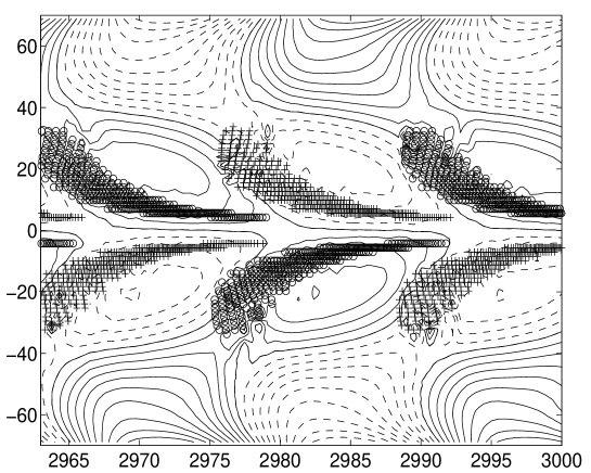
Figure 13: Theoretical butterfly diagram of eruptions for our standard model. The background shows contours of diffuse radial field. Eruption latitudes are denoted by symbols ’o’ and ’+’, indicating negative and positive toroidal field respectively. The dashed contours are for negative $B_{r}$, whereas the solid contours are for positive $B_{r}$. Note that negative toroidal fields give rise to negative radial field near the poles after decaying and vice versa in accordance with Hale’s polarity law.

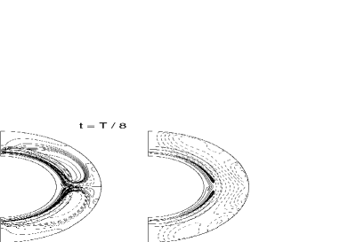
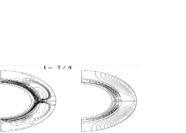
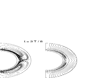
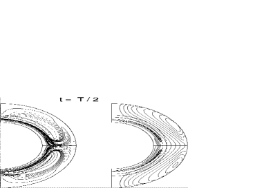
Figure 14: Four snapshots of the toroidal field contours (left panel), and the poloidal field lines (right panel) separated by 1/8^th of the dynamo period $T$. The case $t=0$ is shown in Fig. 8. The line styles are same as in Fig 8.

4.1 The effect of velocity quenching

One important question is whether the equatorward meridional circulation at the base of SCZ should be able to advect the strong toroidal field, working against the magnetic tension. It has been argued by Choudhuri (2003b) that this should be possible if the strong toroidal field is highly intermittent. However, Choudhuri (2003b) concluded that the meridional flow may be barely strong enough to advect the toroidal field. If $B$ becomes larger than some critical value, then the meridional flow may not be able to carry it. We try to capture this effect by checking at intervals of 10 days if the toroidal field exceeds a critical value of 1.5$\times$10⁵ G in a region of thickness 0.11$R_{\odot}$ below a depth of 0.73$R_{\odot}$. Whenever $B$ is larger than this critical value, we reduce the velocity at that grid point by a factor of eight. A butterfly diagram similar to Fig. 13 is produced in this case and is shown in Fig. 15. On comparing Fig. 13 and Fig. 15, we find that this velocity quenching improves the appearance of the butterfly diagram. We saw in Fig. 13 that eruptions for a new half-cycle began at high latitudes before the eruptions at low latitudes stopped for the previous half-cycle, leading to a tail-like attachment in the butterfly diagram. We see in Fig. 15 that this is gone and a new half-cycle begins at the high latitude at about the time when the old half-cycle dies off at the low latitude—in conformity with observational data (see Fig. 6.2 of Choudhuri 2003a).

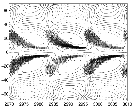
Figure 15: Theoretical butterfly diagram of eruptions for the case presented in §4.1. The various conventions used are the same as in Fig 13.

5 Conclusion

We show that a CDSD model with an $\alpha$ effect concentrated near the surface and a meridional circulation penetrating below the tachocline provides a satisfactory explanation for various aspects of the solar cycle. The helioseismically determined differential rotation is strongest at high latitudes within the tachocline and there is little doubt that the strong toroidal field should be produced there, to be advected by the meridional flow to low latitudes where it erupts. This view, which was first put forth by Nandy & Choudhuri (2002), is a departure from the traditional viewpoint that the toroidal field is produced basically at the same latitude where it erupts. Ironically, this new viewpoint makes the original motivation of Choudhuri et al. (1995) in introducing the meridional circulation somewhat redundant. A standard result of dynamo theory (without any flow in the meridional plane), which was first derived by Parker (1955), is that the product of $\alpha$ and $\partial\Omega/\partial r$ should be negative in the northern hemisphere, to ensure the equatorward propagation of the dynamo wave (see, for example, Choudhuri 1998, §16.5). The tilts of bipolar regions on the solar surface suggest that $\alpha$ should be positive in the northern hemisphere, whereas helioseismology found $\partial\Omega/\partial r$ also to be positive in the lower latitudes. If the strong toroidal field is produced within the tachocline at low latitudes where it erupts, then the simple sign rule would suggest a poleward propagation. Choudhuri et al. (1995) introduced the meridional circulation primarily to overcome this tendency of poleward propagation, forcing the dynamo wave to propagate equatorward. If the toroidal field is produced at high latitudes where $\partial\Omega/\partial r$ is negative, then the dynamo wave should propagate poleward even in the absence of meridional circulation. Although the original motivation of Choudhuri et al. (1995) in introducing the meridional circulation may no longer be so relevant, it has become increasingly clear in the last few years that the meridional circulation plays a crucial role in the solar dynamo. There are indications that the meridional circulation may actually be the time-keeper of the solar cycle (Hathaway et al. 2003). We hope that within the next few years helioseismology will discover the equatorward return flow of meridional circulation and may even be able to establish if this return flow really penetrates below the tachocline, as required by us.

Dikpati & Gilman (2001) and Bonanno et al. (2002) had earlier argued that a pure Babcock–Leighton dynamo with $\alpha$ concentrated near the surface may not give the correct dipolar parity. We have clearly demonstrated that this is not the case. If the poloidal field has sufficient diffusivity to get coupled across the equator, whereas the toroidal field is not able to diffuse across the equator (since turbulent diffusion is suppressed for the strong toroidal field), then we find that the dipolar mode is preferred. We saw in §3.3 that an additional $\alpha$ effect in the interior of SCZ would help in establishing dipolar parity. However, in view of the fact that our knowledge about such an $\alpha$ effect is very uncertain, we felt that it is first necessary to study pure Babcock–Leighton dynamo models with $\alpha$ effect concentrated near the surface alone. Accordingly, we have taken such a dynamo model which gives the correct dipolar parity as our standard model. We have shown in §4 that this standard model explains many aspects of observational data very well. We are right now exploring whether this standard model can explain some other aspects of observational data not discussed by us here. For example, active regions in the northern hemisphere are known to have a preferred negative helicity. A theoretical explanation for this has been provided by Choudhuri (2003b). Our preliminary investigations based on the idea of Choudhuri (2003b) show that our standard model presented in this paper would give the right type of helicity. We are now carrying out more detailed calculations, which will be reported in a forthcoming paper. We may mention that our code can be used for other MHD calculations besides the solar dynamo problem. A modified version of the code has been used to study the evolution of magnetic fields in neutron stars (Choudhuri & Konar 2002; Konar & Choudhuri 2004).

Acknowledgements. Most of our calculations were carried out on Sanḱhya, the parallel cluster computer in Centre for High Energy Physics, Indian Institute of Science. D. N. acknowledges financial support from NASA through SR&T grant NAG5-11873.

References

Babcock, H.W. 1961, ApJ, 133, 572.
Bonanno, A., Elstner, D, Rüdiger, G., & Belvedere, G., 2002, A&A, 390, 673
Braun, D.C., & Fan, Y. 1998, ApJ, 508, L105.
Caligari, P., Moreno-Insertis, F., & Schüssler, M. 1995, ApJ, 441, 886.
Charbonneau, P., Christensen-Dalsgaard, J., Henning, R., et al., 1999, ApJ, 527, 445
Choudhuri, A.R. 1989, Solar Physics, 123, 217
Choudhuri, A.R. 1998, The Physics of Fluids and Plasmas: An Introduction for Astrophysicists, Cambridge University Press, Cambridge.
Choudhuri, A.R., 2003a, in Dynamic Sun, ed B.N. Dwivedi, Cambridge University Press, 103.
Choudhuri, A.R., 2003b, Solar Phys, 215, 31
Choudhuri, A.R., & Dikpati, M. 1999, Solar Physics, 184, 61
Choudhuri, A.R., & Gilman, P.A. 1987, ApJ, 316, 788
Choudhuri, A.R., & Konar, S., 2002, MNRAS, 332, 933
Choudhuri, A.R., Schüssler M., & Dikpati M. 1995, A&A, 303, L29
Dikpati, M., & Charbonneau, P. 1999, ApJ, 518, 508
Dikpati, M., & Choudhuri, A.R. 1994, A&A, 291, 975
Dikpati, M., & Choudhuri, A.R. 1995, Solar Physics, 161, 9
Dikpati, M., & Gilman, P.A. 2001, ApJ, 559, 428
D’Silva, S., & Choudhuri, A.R. 1993, A&A, 272, 621
D’Silva, S., & Howard, R.F., 1993, Solar Physics, 148, 1
Durney, B.R. 1995, Solar Physics, 160, 213
Durney, B.R. 1996, Solar Physics, 160, 231
Durney, B.R. 1997, ApJ, 486, 1065
Fan, Y., Fisher, G.H., & DeLuca, E.E. 1993, ApJ, 405, 390
Ferriz-Mas, A., Schmitt, D., & Schüssler, M., 1994, ApJ, 289, 949
Giles, P.M., Duvall, T. L., Jr., Kosovichev, A. G., & Scherrer, P. H., 1997, Nature, 390, 52
Gilman, P.A. 1983, ApJS, 53, 243
Gilman, P.A. 1986, in Physics of the Sun, Vol 1, 95-160, Dordrecht, D. Reidel Publishing Co.
Hathaway, D. H., Nandi, D., & Wilson, R. M., Reichmann, E.J., 2003, Astrophys. J., 589, 665
Konar, S., & Choudhuri A.R., 2004, MNRAS, 348, 661
Küker, M., Rüdiger, G. & Schultz, M. 2001, A&A, 374, 301
Leighton, R.B. 1969, ApJ, 156, 1
Longcope, D. & Choudhuri, A.R., 2002, Solar Physics, 205, 63
Miesch, M. S., Elliott, J. R., Toomre, J., et al. 2000, ApJ, 532, 593
Nandy, D., 2002 Ap&SS, 282, 209
Nandy, D., 2003, Modelling the Solar Magnetic Cycle, PhD Thesis, Dept of Physics, Indian Institute of Science
Nandy, D., & Choudhuri, A.R. 2000, J. Astrophys. Astron., 21, 381
Nandy, D., & Choudhuri, A.R. 2001, ApJ, 551, 576
Nandy, D. & Choudhuri, A.R., 2002, Science, 296, 1671
Parker, E.N. 1955, ApJ, 122, 293
Schmitt, D., & Schüssler, M., 1989, A&A, 223, 343
Schou, J., Antia, H. M., Basu, S., et al, 1998, ApJ, 505, 390
Steenbeck, M., & Krause, F., Rädler, K.H., 1966, Z. Naturforsch., vol-21a, 369
Wang, Y.-M., Nash, A.G., & Sheeley, N.R. 1989a, ApJ, 347, 529
Wang, Y.-M., Nash, A.G., & Sheeley, N.R. 1989b, Science, 245, 712
Wang, Y.-M., Sheeley, N.R., & Nash, A.G. 1991, ApJ, 383, 431