The Luminosity, Stellar Mass, and Number Density Evolution of Field Galaxies of Known Morphology from $z=0.5-3$

Abstract

The evolution of rest-frame B-band luminosities, stellar masses, and number densities of field galaxies in the Hubble Deep Field North and South are studied as a function of rest-frame B-band morphological type out to redshifts $z\sim 3$ using a sample of 1231 I $<27$ galaxies with spectroscopic and photometric redshifts. We find that the co-moving number, and relative number, densities of ellipticals and spirals declines rapidly at $z>1$, although examples of both types exist at $z>2$. The number and number fraction of peculiar galaxies consistent with undergoing major mergers rises dramatically and consistently at redshifts $z>2$. Through simulations we argue that this change is robust at the 4 $\sigma$ level against morphological k-corrections and redshift effects. We also trace the evolution of rest-frame B-band luminosity density as a function of morphology out to $z\sim 3$, finding that the luminosity density is steadily dominated by peculiars at $z>1.5$ with a peak fraction of 60-90% at $z\sim 3$. By $z\sim 0.5$ B-band luminosity fractions are similar to their local values. At $z\sim 1$ the B-band luminosity densities of ellipticals and spirals are similar, with a combined contribution of $\sim$ 90% of the total luminosity at $z<1$. The stellar mass density follows a similar trend as the luminosity density, with some important exceptions. At high redshifts, $z>2$, 60-80% of stellar mass appears attached to peculiars, while at $z<1$, 80% - 95% of stellar mass is attached to ellipticals and spirals. The total integrated stellar mass density of peculiars slightly declines at lower redshift, suggesting that these systems evolve into normal galaxies. In contrast to the luminosity density, the stellar mass density of ellipticals is greater than spirals at $z<1$, and the stellar masses of both types grow together at $z<1$, while number densities remain constant. From a structural analysis of these galaxies we conclude that galaxy formation at $z>2$ is dominated by major merging, while at $z<1$ the dominate modes are either minor mergers or quiescent star formation produced by gas infall. Finally, at $z\sim 1.5$ the co-moving luminosity, mass, and number densities of spirals, ellipticals and peculiars are nearly equal, suggesting that this is the ‘equilibrium’ point in galaxy evolution and an important phase transition in the universe’s history.

1. Introduction

Understanding how and when nearby galaxies formed and evolved into their present physical and morphological states is a major goal of contemporary astrophysics. Most mass in the universe is likely attached to galaxies, thus understanding the origins of these systems is central to any ultimate theory of how structure developed. Galaxy formation is now at the fore-front of cosmology, as many major cosmological questions and parameters appear to be known with some certainty (Spergel et al. 2003). There is luckily progress on this front. The nearby bright galaxy population, defined as galaxies brighter than M${}_{\rm B}<-20$, are becoming fairly well characterized with recent surveys such as 2dF and the Sloan Digital Sky Survey (SDSS) (e.g., Kauffmann et al. 2003; Bell et al. 2003), and will become even more so after the SDSS is completed. Thus far, Sloan and others has argued that $\sim 30$% of the luminosity in the nearby universe originates from early-type galaxies, with an even higher fraction of contemporary stellar mass in these evolved systems (e.g., Fukugita, Hogan & Peebles 1998; Blanton et al. 2001; Hogg et al. 2002; Baldry et al. 2003). The nearby bright galaxy population is also clearly bimodal with a large population of old massive systems, and a large population of less massive galaxies with younger stellar populations (Kauffmann et al. 2003; Baldry et al. 2004). The morphological distributions of nearby galaxies is however, not as well studied. An analysis of the largest morphological catalog of galaxies, the “Third Reference Catalogue of Bright Galaxies” (de Vaucouleurs et al. 1991), show that approximately 75% of all galaxies with M${}_{\rm B}<-20$ are spirals, while about 23% are ellipticals and the remainder are irregular galaxies (see also Marzke et al. 1994). How and when did this $z\sim 0$ morphological distribution come into place, and how is this related to the development of stellar populations? We can answer these questions directly by looking at galaxies at high redshift with the Hubble Space Telescope (HST).

Deep ground based and Hubble Space Telescope (HST) imaging (e.g., Glazebrook et al. 1995; Driver et al. 1995; Madau et al. 1996; Brinchmann et al. 1998; Steidel et al. 1999; Conselice et al. 2003; Dickinson et al. 2003) has revealed basic evolutionary trends in the evolution of field galaxies. Lilly et al. (1995) argue from an I-band selected survey that the luminosity density of galaxies, and thus the star formation rate, increases as a function of redshift out to $z\sim 1$. Madau et al. (1996) followed this up by examining the rest-frame UV luminosity densities out to $z\sim 4$, demonstrating that the star formation rate remains high out to these redshifts. Many of these star forming galaxies were found to be irregular in appearance to $z=1$ as shown by HST imaging of these fields (e.g., Brinchmann et al. 1998). Complementary to this work is investigating the stellar mass evolution of galaxies (e.g., Dickinson et al. 2003; Rudnick et al. 2003; Fontana et al. 2003; Glazebrook et al. 2004). These studies find that at $z\sim 3$, only approximately 10% of modern stellar mass is formed, which rises to $\sim$ 50-75% at $z\sim 1$. If these results are not biased by missing a substantial population of massive galaxies, or by cosmic variance, then galaxy formation is a gradual process that occurs over the age of the universe. It appears that we are coming to an agreement concerning when galaxies in our universe formed and the next step is determining how this formation occurred.

There are at least three main methods for how galaxies can form: major mergers (with mass ratios of 3:1 or lower), minor mergers (with mass ratios of 3:1 or higher), and gas accretion from the intergalactic medium. Understanding which of these processes is occurring requires examining the internal features of galaxies either through high resolution imaging or integral field spectroscopy. It has been known for some time that a significant fraction of galaxies in the distant universe have irregular/peculiar morphologies which may be signs of merger activity (e.g., Glazebrook et al. 1995; Driver et al. 1995; Abraham et al. 1996). These early studies were however limited as many did not have redshifts, and thus could not trace the cosmic evolution of galaxy structure. Recently, van den Bergh et al. (2000), Brichmann & Ellis (2000), van den Bergh, Cohen & Crabee (2001), and Kajisawa & Yamada (2001) who use redshift information, argued that there is a real evolution in morphology as a function of time. Van den Bergh et al. (2000) argued that very few ellipticals and spirals exist at redshifts $z>1.5$ and other morphological properties seem to change slowly from $z\sim 1.5$ until today. We know that this change in morphology at high redshift is not the result of so-called morphological k-corrections, where galaxies look more irregular at shorter wavelengths (Windhorst et al. 2002; Papovich et al. 2003). Conselice et al. (2003) use HST imaging of the HDF to argue that galaxy formation for the most massive systems is dominated by merging and calculates the basic merger history of field galaxies. By uncovering how galaxies and stellar mass form as a function of morphological type and structure we can begin to determine the formation modes of galaxies.

To perform this analysis we use the Hubble Deep Field North and South WFPC2 and NICMOS images with the CAS (Concentration, Asymmetry, Clumpiness) classification system (Conselice 2003) combined with eye-ball morphology, color, stellar mass, and luminosity information. In this paper we characterize the evolution of stellar masses, luminosity densities, and number densities as a function of morphology. We show that at the highest redshifts most stellar mass is attached to peculiar galaxies. At lower redshifts the amount of stellar mass in peculiars gradually decreases while the amount in ellipticals and spirals gradually increases, verifying on a longer time-scale, the results of Brinchmann & Ellis (2000) who find a similar trend for galaxies at $z<1$. One basic result is that at $z\sim 1.5$ the co-moving densities, co-moving B-band luminosities and co-moving stellar mass densities are nearly equal for peculiars, disks, and ellipticals. This is the same epoch where disks and ellipticals first appear morphologically in abundance. At redshifts $z>1.5$ peculiar galaxies, which we argue based on the CAS systems are mergers, increasingly dominate number, luminosity, and mass densities out to $z\sim 3$. At $z<1.5$, we find, similar to Brinchmann et al. (1998) and Brinchmann & Ellis (2000), that ellipticals and disks dominate in number, luminosity and stellar mass density. We further conclude that major mergers are the dominate mode for forming the most massive galaxies at $z>1.5$ while minor mergers and gas accretion from the intergalactic medium are the likely cause of star formation and stellar mass assembly at $z<1.5$.

This paper is organized as follows: §2 is a description of the data used in this paper and the morphological techniques used to study galaxies in the two Hubble Deep Fields. §3 is the description of our analysis while §4 & §5 are a discussion and a summary of our results. We assume a cosmology with H₀ = 70 km s^-1 Mpc^-1, $\Omega_{\Lambda}$ = 0.7 and $\Omega_{\rm m}$ = 0.3 throughout.

2. Data and Analysis Method

2.1. Images

Our basic imaging data are the Hubble Deep Field North WFPC2 (Williams et al. 1996) and NICMOS fields (Dickinson et al. 2000, 2003) (hereafter HDF-N) as well as the Hubble Deep Field South WFPC2 images (hereafter HDF-S) (Casertano et al. 2000) and the VLT near infrared ISAAC images of the HDF-S (Labbé et al. 2003). In these two fields, we use the following broad-band filters: F450W (hereafter B₄₅₀), F606W (hereafter V₆₀₆), F814W (hereafter I₈₁₄) from WFPC2, and F110W (hereafter J₁₁₀) and F160W (hereafter H₁₆₀) from NICMOS for the HDF-N. The ISAAC data for the HDF-S includes J_s, H and K_s band imaging over a 2.5′$\times$ 2.5′  area to 3$\sigma$ AB magnitude depths of 26.8, 26.2 and 26.2, respectively. These data are used for the structure analyses, and for deriving photometric redshifts and other photometric and structural properties that we use throughout this paper. Ground based infrared photometry for both the HDF-N and HDF-S galaxies are also included in these measurements (e.g,. Dickinson et al. 2003).

2.1.1 Catalogs of Galaxies

The galaxies in the two Hubble Deep Fields were selected using SExtractor (Bertin & Arnouts 1996). For the HDF-S the detection was done on the I₈₁₄ band image, while a combined J₁₁₀+H₁₆₀ image was used for the HDF-N. We then match these catalogs to all further data, including photometric redshifts. We also use these catalogs for our morphological analyses. From these catalogs, a total of 1288 objects were detected in the Hubble Deep Field North and 1293 in the HDF-S. We classify all of these 2581 objects, in the two HDFs, although only a fraction have meaningful morphological parameter measurements. To avoid problems associated with fainter and less resolved galaxies we do a cut on galaxies to remove systems with apparent magnitudes I$>27$ from our analyses. Galaxies fainter than this generally cannot have their morphological parameters measured with any certainly, due to the their low-S/N and resolution (Conselice et al. 2000a, Conselice 2003; §2.3).

2.1.2 Redshifts - Spectroscopic and Photometric

There are spectroscopic redshifts available for galaxies in the HDF-N, with the bulk from the surveys of Cohen et al. (2000) and Steidel et al. (2003), but other sources as well. These redshifts are typically for galaxies brighter than $R=25.5$, although some fainter sources have redshifts. These redshifts are discussed in detail in Budavári et al. (2000). For the HDF-S, there are 43 redshifts from the VLT study of Sawicki & Mallen-Ornelas (2003). The Sawicki & Mallen-Ornelas galaxies are all at $z<1$ however. For the remaining galaxies in these fields, we use photometric redshifts as derived by Budavári et al. (2000) for the HDF-N galaxies, and by the Stony Brook photometric redshift group (e.g., Yahata et al. 2000) and the FIRES team (e.g., Rudnick et al. 2003) for the HDF-S fields. The photometric redshifts for Rudnick et al. (2003) are however limited in number and we use the Stony Brook redshifts whenever there is no spectroscopic redshift or FIRES photometric redshift. The accuracy of the photometric redshifts for the HDF-N are discussed in detail in Budavári et al. (2000). For the HDF-S, no comparison between the photometric redshifts of the Lanzetta group and the spectroscopic redshifts have yet been done. Figure 1 shows this comparison for galaxies with spectroscopic redshifts in the HDF-S field. The scatter between the photometric redshift and the spectroscopic redshifts is $\sigma$ = 0.08 with an average offset of 0.06 and an average ($\delta z/z)=0.11$. This is a fairly good accuracy, and suggests that the other photo-zs are likely reliable, on average, within this uncertainty. However as photo-zs are less accurate at fainter magnitudes, they are likely less reliable for less luminous and/or more distant galaxies. We compute rest-frame properties of these galaxies, including their absolute blue magnitudes (M_B, rest-frame colors, and sizes) using these redshifts (see also Dickinson et al. 2003).

2.2. Photometric Properties

Throughout this paper we use the broad-band HST and ground based photometry to determine rest-frame absolute magnitudes, colors, and sizes for our sample. The photometric properties of galaxies are determined through interpolating rest-frame values of M_B and $(B-V)$. No K-corrections are computed as we directly measure these values from the SED and knowledge of the redshift for each galaxy. See Dickinson et al. (2003) and Conselice et al. (2003) for more details on how these interpolations are done.

2.3. Morphological Classifications

We performed eye-ball classifications for all 2581 galaxies in the observed I₈₁₄ band, as well as in the H₁₆₀ for the HDF-N. Based on these images a classification was made. Each galaxy was put into one of six categories: star, elliptical, early-type disk, late-type disk, edge-on disk, irregular, merger/peculiar, and unknown/too-faint. These classifications are very simple and are only based on appearance. No other information, such as colors or redshifts were used when determining types. We discuss in §3.1 biases due to redshift effects and morphological k-corrections. Ellipticals, early-type disks and late-type disks were classified based on the presence of apparent bulge and disk components through the following criteria:

1. Ellipticals: If a galaxy appeared to be centrally concentrated with no evidence for a flatter, lower surface brightness, outer structure it was classified as an elliptical.

2. Early-type disks: If a galaxy contained a central concentration with some evidence for lower surface brightness outer light, it was classified as an early-type disk.

3. Late-type disks: Late-type disks are galaxies that appear to have more outer low surface brightness light than inner concentrated light.

4. Irregulars: Irregulars are galaxies that appear to have no central light concentration and a diffuse structure, sometimes with clumpy material present.

5. Peculiars: Peculiars are systems that appear to be disturbed or peculiar looking. These galaxies are possibly in some phase of a merger (Conselice et al. 2003) and are common at high redshifts.

6. If a galaxy was too faint for any reliable classification it was placed in the unknown/too-faint category. Often these galaxies appear as smudges without any structure. These could be disks or ellipticals, but their extreme faintness precludes a reliable classification. Often, a system appeared very faint, but large scale peculiarities, such as warping and non symmetrical structure could be detected by eye. If any of these systems displayed this peculiarity it was placed into the peculiar category.

The usefulness of this type of morphological classification is questionable (e.g., Conselice 2003) since Hubble types, and other eye-based classifications, are subjective. There is also the issue that fainter galaxies will be more difficult to classify, although classifications in the HDFs are on average possible to I = 27 (Conselice et al. 2000a). This is fainter than the limit used in Abraham et al. (1996), whose use a I = 25 limit. Our analyses are based on definitive classifications of broad types, with a generous ’unclassifiable’ option, and these should not be affected significantly by morphological classification biases. It is clear from the data that to I = 27 classifications can be performed for the majority of galaxies. Between I = 26 and I = 27, 38% of systems are unclassifiable, this rises to 61% between I = 27 and I = 28. We thus use the limit I = 27 for obtaining a morphological classification for the majority of galaxies in the HDFs. To test the reliability of this classification, we do a series of simulations of nearby galaxies (§2.6.1) and HDF-N galaxies between $z\sim 0.5-0.8$ placing them at higher redshifts. When we reclassify these galaxies after simulation we find that most ($\sim$ 70%) with magnitudes $I=26-27$ are still classifiable by eye into their original types, justifying our use of this magnitude limit. Note that at $I=27$, quantitative classifications are also possible, but require corrections due to surface brightness dimming (Conselice et al. 2000a; §2.6.1). We also repeat this eye-ball classification for the HDF-N using the NIR H₁₆₀ band images to test for effects of morphological k-corrections (§2.6) and to obtain a rest-frame B-band classification for the HDF-N sample.

2.4. CAS Parameters

To quantify the structural features of galaxies in the HDFs, we use the concentration, asymmetry and clumpiness (CAS) system described in detail in Conselice (2003). In the CAS system the concentration index ($C$) is a measure of how centrally concentrated or compact a galaxy is (Bershady et al. 2000). Based on empirical correlations the concentration index is a measure of the form, and scale of a galaxy (i.e., its mass). Concentrations correlate fairly well with the absolute magnitude of a galaxy and its bulge to disk ratio (Conselice 2003). The asymmetry index ($A$), first measured by Schade et al. (1995), Abraham et al. (1996) and Conselice (1997) is a measure of the global distortion in a galaxy from a completely symmetric structure, and is a good method for indicating galaxies undergoing major mergers (Conselice et al. 2000a, 2000b; Conselice et al. 2003). The clumpiness index, $S$, correlates with the amount of star formation in a galaxy, as shown by its fairly strong correlation with H$\alpha$ fluxes and broad-band colors (Conselice 2003). There are many issues concerning how these parameters are measured, which are discussed at length in Conselice et al. (2000a), Bershady et al. (2000) and Conselice (2003).

2.4.1 Contamination from Galaxies - Segmentation Maps

Since the CAS system is model independent and works in batch mode, the catalogs for the various HDFs were fed into an IRAF based program that computes CAS parameters and Petrosian radii for each galaxy (see Conselice 2003). Before we ran any of the CAS programs, we performed several pre-analysis quality control steps. The most important of these was to minimize as much as possible contamination from neighboring galaxies. This was done was by creating SExtractor (Bertin & Arnouts 1996) segmentation maps that reveal unambiguously pixels belonging to each galaxy. These maps are created during the SExtractor detection process. The form of the segmentation map is such that every pixel is valued either zero or has a integer value, corresponding to a catalog entry, that reveals which galaxy that pixel belongs. Based on these maps, we isolated each galaxy’s segmentation area and placed all light from other galaxies to the background level and noise before computing the CAS parameters. Systems which are merging may be artificially separated by this process into two separate galaxies. This is largely not a problem however as galaxies which are undergoing mergers are asymmetric with, or without, the presence of the other galaxy. The only concern about these galaxies is that they might be double counted when considering the number of mergers (see Conselice et al. 2003). We are also not biasing asymmetry measurements by replacing the light from nearby galaxies with the background, and therefore potentially not retrieving the underlying light from the galaxy being measured. The reason for this is that the asymmetry computation is heavily weighted towards the brightest parts of a galaxy, and any faint outer light contributes very little to the measurement (Conselice 2003).

There are many other technical issues that are involved in applying an automated and quantitative approach such as measuring CAS parameters. These issues include correcting for noise and defining the radius and center by which these parameters are measured. The noise in the HDF-N and HDF-S WFPC2/NICMOS images is enhanced near the edges of the frames, and thus we remove these systems from our analyses. To deal with noise in a general sense we follow the procedure outlined in Conselice et al. (2000a, 2003) for understanding and accounting for systematics presented by the background. We further follow the techniques in these papers when accounting for radii and centering routines when computing the CAS parameters. We give only a brief description of these procedures here and refer the reader to previous papers for detailed explanations for how CAS parameters are computed.

2.4.2 Background Removal

One critical component to understanding and correct for when measuring CAS parameters is the presence of background noise. This noise originates from read noise, photon counts from background light, and any intrinsic variations of this background within a small sky area. Our background correction method as outlined in Conselice et al. (2003), will correct for both correlated and uncorrelated noise, assuming that in either case it is also present where the galaxy itself is found. As noted in Conselice et al. (2003) there are several problems to this methodology, most importantly the fact that the sky varies across these images, particularly in the NICMOS bands (Conselice et al. 2003). We obtain a partial solution to this problem by computing the CAS parameters using several background areas across each WFPC2 and NICMOS image. This gives us an understanding of how the background light contributes to errors in our measurements, as each CAS run gives us a slightly different set of parameters depending on the background area chosen. After measuring CAS values using these different backgrounds we find that the statistical variation in the computation of these parameters across images is smaller than the measurement errors. This effect therefore does not contribute significantly to the error budget of our CAS measurements.

2.4.3 Radii

We use in this paper the 1.5 $\times$ r$(\eta=0.2)$ inverted Petrosian radius described and calibrated in detail in Bershady et al. (2000), Conselice et al. (2000a) and Conselice (2003) to measure CAS parameters. Briefly, the inverted Petrosian radius is the radius where the surface brightness in an annulus at that radius is a given fraction of the surface brightness within the radius. Our use of $\eta=0.2$ to define the radius of our galaxies is the same as that used by the Sloan Digital Sky Survey to measure magnitudes (e.g., Blanton et al. 2001). Based on simulations, it can be shown that for most popular galaxy light profiles, such as exponential, gaussian, and de Vaucouleur, the Petrosian radius, defined this way, contains $\sim 99$% of the light from these systems. The CAS program also measures the half-light radii of these galaxies, within the 1.5 $\times$ r$(\eta=0.2)$ radius.

2.4.4 Rest-Frame B-band CAS Values

Using the wavelength coverage of the WFPC2 bands, we are able to determine the rest-frame B-band morphologies of our sample in both the HDF-N and HDF-S out to $z\sim 1.2$. We can further compute rest-frame B-band CAS parameters out to $z\sim 2.5$ using the NICMOS HDF-N imaging. We compute rest-frame B-band CAS parameters and radii by linearly interpolating between the values measured in the observed HST wavebands, that straddle the observed wavelength of the B-band, at a given redshift. For galaxies at $z>2.5$, in the HDF-N, we use the observed H₁₆₀ band morphologies and radii.

2.5. Stellar Masses

The stellar masses we use are from the analyses of Papovich et al. (2001), Papovich (2002) and Dickinson et al. (2003) for the HDF-N. We calculate the stellar masses for the HDF-S using photometry from WFPC2 optical imaging and infrared imaging form the FIRES survey (e.g., Labbé et al. 2003) using the techniques from Papovich et al. (2001). The stellar masses in the north field are computed through spectral energy distributions using Hubble Space Telescope WFPC2 imaging in the U₃₀₀, B₄₅₀, V₆₀₆ and I₈₁₄ bands, as well as NICMOS imaging in the J₁₁₀ and H₁₆₀ bands. A deep K-band image of the HDF-N taken with the Kitt Peak National Observatory 4 meter is also included. To determine the stellar masses of the galaxies in both the north and the south their SEDs were fit by various star formation histories with different metallicities and internal extinction values derived from Bruzual & Charlot (2003) stellar population synthesis models. After a best fit to the observed SED is found, the M/L ratio is derived and the stellar mass is computed based on this. The major parameters for the fitting are the age of the stellar population and the star formation time-scale. There are several different possible initial mass functions and star formation histories that can be used to do this modeling of M/L ratios. We however use models where the IMF is Salpeter and ranges from 0.1 to 100 M${}_{\odot}\,$, the metallicity is solar, and the star formation history monotonic. We also use similar SEDs used to computed the k-corrections for the photo-zs discussed in §2.1.2. The best model is then selected by the $\chi^{2}$ technique with Monte Carlo simulations employed to determine the 68% confidence or error intervals on the stellar masses after randomly including changes within the photometry error budget. For more details on this process see Papovich et al. (2001) and Dickinson et al. (2003).

2.6. Biases

2.6.1 Redshift Effects and Morphological K-Corrections

It is important to understand what effects redshift will have on the quantitative values of our galaxy classifications, including the CAS parameters, particularly if redshift creates a systematic effect of either lowering or rising the threshold for placing an object into one of the Hubble sequence bins. This effect has already been explored by Conselice et al. (2000a), Conselice (2003) and Conselice et al. (2003) although we re-examine this in more detail here in a empirical way here and in §3.1.1. There are two major effects produced by redshift - the dimming of galaxies and the morphological k-correction.

To determine how various normal galaxy morphologies change solely due to redshift effects, that is surface brightness dimming, we simulate rest-frame optical images of nearby Hubble types from the Frei et al. (1996) digital catalog of galaxies (see also Conselice 2003) by placing them at higher redshifts. By doing this we are able to determine how the morphological properties of galaxies change solely due to redshift. We analyze these simulations by performing the exact same CAS runs on these simulated galaxies as we did on the galaxies in the HDFs themselves. Thus, by comparing the CAS parameters for the $z\sim 0$ sample to how their values change at $z>1$, we can determine the effects of redshift on the measurement of CAS parameters, which we can compare to the observed evolution to determine the true change in CAS values from low to high redshift. We find that the most significant changes occur at redshifts $z>1.5$, particularly for the most asymmetric and clumpy galaxies. Table 1 lits the changes in the CAS parameters at different redshifts.

Galaxies also look different at different wavelengths, which is a result of the so-called morphological k-correction (Windhorst et al. 2002; Papovich et al. 2003). Generally, galaxies appear as later types when viewed at bluer wavelengths, as star formation is more visible and older stellar populations are fainter at shorter wavelengths. Although we generally use rest-frame B-band morphological classifications in this paper, there could be some biases, particularly at high redshifts where the rest-frame I₈₁₄ band samples the rest-frame UV for these systems. Figure 2 plots classifications in the H₁₆₀ and I₈₁₄ bands versus each other. The line through the middle overlaps those systems which have the same classification in both bands.

Figure 2 demonstrates that there are some morphological biases between the two bands. The most common disagreement is that there are more systems classified as ’too faint’ in the H-band than in the I-band. This results from these systems, which are most commonly ellipticals and peculiars, being too faint in the H₁₆₀ band due to the shorter exposure time used to obtain the NICMOS imaging (Dickinson et al. 2000). Otherwise, the most common misclassifications are what we would expect. For example, there are 13 systems classified as an early type spiral (eS) in the I₈₁₄ band which are classified as elliptical in the H₁₆₀, and there are nine systems classified as a late type spiral (lS) in I₈₁₄ which are classified as early-type spirals in H₁₆₀. Most of these systems are at low redshift, where disks and ellipticals are found in abundance. We are thus not likely biased by using the I₈₁₄ band in determining classifications, particularly peculiars, which remain peculiar at all wavelengths.

2.6.2 Galaxy Selection

There are many selection effects which we discuss throughout this paper. The most obvious is that we use a I₈₁₄ $<27$ magnitude selection for galaxies in our analysis. This selection allows us to determine with accuracy the morphologies of galaxies under study, but removes optically faint galaxies at high redshift from our sample. As such, it is important to determine the characteristics of this selection for our analysis. The first step in understanding biases from the I₈₁₄ $<27$ selection is to determine the redshift distribution of our I${}_{814}<27$ galaxy sample in both the HDF-N and HDF-S (Figure 3). As can be seen, the peak in the distribution is at $z\sim 1$, with a smaller peak at higher redshifts around $z\sim 2$.

To determine how faint we can go in our analysis without missing objects, we investigate how absolute magnitudes vary with redshift (Figure 4). At redshifts $z<2$ all galaxies brighter than M${}_{\rm B}=-20$ appear to be detected without a significant incompleteness. As we sometimes use this magnitude limit in this paper, we can draw global morphological conclusions at redshifts $z<2$ for galaxies with $M_{\rm B}<-20$. At $z>2$, the I${}_{814}<27$ limit is likely incomplete and we cannot be confident that we are not missing some fraction of the galaxy population. Unless otherwise stated, we use the I${}_{814}<27$ limit in our analysis.

The fact that we are not missing galaxies at $z<2$ can also be seen in another way by examining Figure 5 which plots the apparent magnitudes of all HDF-S and HDF-N galaxies, as a function of redshift, out to $z\sim 3$ with the I${}_{814}<27$ limit imposed. The solid, short dashed and long dashed lines are the expected apparent magnitude of M${}_{\rm B}=-20$ ellipticals, Sa and Sc galaxies, respectively, as a function of redshift. The value M${}_{\rm B}=-20$ is roughly the value of L^∗ for modern galaxies. The apparent magnitudes were computed through the formula: I₈₁₄ = M_I + DM + K, where M_I is the absolute I-band magnitude of each type computed from Fukugita et al. (1995), DM is the distance modulus, and K is the K-correction. K-corrections for each type were computed from SEDs presented in Poggianti (1997). No evolutionary corrections have been applied to these magnitudes, which would only make the galaxies brighter, especially the ellipticals. As a note, the recently discovered evolved massive galaxies in the HDF-S by Franx et al. (2003) all would be included in our analysis as they have magnitudes $I<27$, and are very bright in optical magnitudes with M${}_{\rm V}=-23$ to M${}_{\rm V}=-25$ (van Dokkum et al. 2003) and with M${}_{\rm B}<-20$.

3. Analysis

3.1. The Evolution of Number Densities

The first cut at a basic morphological analysis involves examining how our eye-ball estimates of galaxy types are distributed with redshift. Examining the raw numbers of ellipticals and spirals as a function of type reveals a deficit of ellipticals and spirals at redshifts larger than $z\sim 1.5$ (Figures 6 & 7). There is a gradual decline in the numbers and relative numbers of normal galaxies at $z>1$ as peculiar galaxies become the dominate population. This change remains when we redo the entire classification independently using the H₁₆₀-band images of the HDF-N, which allows us to sample the rest-frame optical to $z\sim 2.5$. Thus, this change is not solely due to observing galaxies in the rest-frame ultraviolet at $z>1.5$ where galaxies can looked different than in the optical (Windhorst et al. 2002). Previous studies (e.g., van den Bergh et al. 2001) were not able to make this claim.

To argue that this change occurs, which we call the galaxy structure-redshift relationship (Conselice 2004), we compute the number of ellipticals and spirals in equal co-moving volumes of $\sim 1131$ Mpc³ arcmin^-2 (Figure 6) for both a I$<27$ limit and a M${}_{\rm B}<-20$ limit. Figure 6 shows that there appears to be a gradual drop in the co-moving density of both spirals and ellipticals at higher redshifts for both selections. The computed co-moving densities for the I$<27$ sample are listed in Table 2. Note that this drop is seen in both the HDF-S and HDF-N, thus it is unlikely to be purely the result of cosmic variance. The drop-off in number becomes more pronounced when we consider only those systems that are brighter than M${}_{\rm B}=-20$. Note that this change is gradual, and does not occur instantaneously, but is most rapid between $1<z<2$.

This can be seen further from Figure 7 which shows the relative fraction of ellipticals, spirals, peculiars, and galaxies too faint for classification, and how their relative densities evolve as a function of redshift. This figures remains largely identical when using the M${}_{\rm B}=-20$ limit. The most notable trend in Figure 7 is the gradual increase in the fraction of galaxies with peculiar morphologies at higher redshifts, with a corresponding decrease in the fraction of ellipticals and spirals. There is also a general relative increase with redshift in the fraction of galaxies too faint for classification in all three images. From Figures 6 & 7 it also appears that there are galaxies that morphologically appear as disks and ellipticals at redshifts $z>1.5$, although the numbers are small (cf. Conselice et al. 2004). Finally, we note that at $z\sim 1.5$ the relative number density of ellipticals, disks and peculiars is relatively similar.

3.1.1 Is the decline in Hubble Types at $z>1.5$ real?

The decline in Hubble types at $z>1.5$ has been noted before (van den Bergh et al. 2001; Kajisawa & Yamada 2001), but its suddenness deserves further attention and a careful analysis. One aspect of this that has not been examined is how much of the drop in normal galaxies is due to redshift effects. To answer this question we simulate galaxies that are at z$\sim 0.65$ in the HDF to how they would appear at $z\sim 1.5$. This simulation is done following the procedure outlined in Conselice (2003) and Conselice et al. (2003). In summary, the procedure is to take the observed V₆₀₆-band HDF-N image, which corresponds to rest-frame B-band for objects at $z\sim 0.65$, and reduce it in resolution and signal to noise to match how these $z\sim 0.65$ galaxies would appear in NICMOS images of the Hubble Deep Field North if they were at $z\sim 1.5$. By doing this experiment we can determine what fraction of spirals and ellipticals are identifiable at this redshift. Note that we use the NICMOS HDF-N H₁₆₀ observational details for this simulation as this filter samples rest-frame optical light at $z\sim 1.5$. After carrying out this simulation, we re-classified in the same manner as described in §2.3 all galaxies originally in the redshift range 0.5 - 0.8, simulated to how they would appear at $z\sim 1.5$. Between redshifts $z\sim 0.5$ and $0.8$ in the HDF-N there are 130 galaxies brighter than M${}_{\rm B}=-19$, of which 35 are classified as ellipticals and 44 as spirals. When we perform the $z\sim 1.5$ simulation and reclassify all objects, we find that 28 of the ellipticals and 29 of the spirals are still identifiable as such. This gives us a detection fraction, f_det, of 0.8 for ellipticals and 0.66 for spirals.

To determine the significance of the drop in ellipticals and spirals at $z\sim 1.5$ we first must determine the systematic effects of redshift on the detectability of these simulated galaxies. Since the drop off in Hubble types occurs at roughly $z\sim 1$, we take the average number, per co-moving Gpc³, of ellipticals and spirals at redshifts $z<1$. We then multiply these densities by the detection fraction from our simulation to determine the number of spirals and ellipticals we would expect to find at $z\sim 1.5$, if no morphological, luminosity, or number density evolution were occurring. The numbers in our fiducial $\sim$ 1131 Mpc³ co-moving volume we expect to find at $z\sim 1.5$ are $\sim 24$ ellipticals and $\sim 26$ spirals. Since we find only three ellipticals and three spirals in this redshift range, there is clearly a significant difference between the number of Hubble types expected and those found. The formal significance of this drop is 4.2 $\sigma$ for the ellipticals and $\sim 4.6$ $\sigma$ for spirals. As we have considered all redshift effects: morphological k-corrections, dimming and resolution, in this calculation we can conclude with confidence that the drop in Hubble types seen at $z\sim 1.5$ is likely real.

The gradual increase of peculiar galaxies at the expense of normal Hubble types is circumstantial evidence that at least some fraction of modern spirals and ellipticals originate from peculiar galaxies (see Conselice et al. 2003; cf Brinchmann & Ellis (2000) for objects at $z<1$). There appears to be a relatively similar number of spirals and ellipticals at $z<1$ in both the HDF-N and HDF-S. At redshifts $z\sim 1.5-2.5$ where the H₁₆₀ data is sampling the rest-frame optical light from these galaxies, we sill find that the fraction of peculiars increases at the expense of Hubble types. The galaxy population is however evenly distributed in co-moving number densities for all types at $z\sim 1.5$. This appears to be the equilibrium point between the number of spirals, ellipticals and peculiars, which breaks down at higher and lower redshifts.

We see similar number density trends in the Hubble Deep Field North and South, although we must deal with the issue of cosmic variance. Having two field effectively reduces the effects of cosmic variance by a factor of two (Somerville et al. 2004). It is difficult to quantify this for the different galaxy types in the HDFs which have different clustering scale lengths. We can investigate this for the Lyman-Break galaxies in the HDFs however. The relative cosmic variance (Somerville et al. 2004) for LBGs in one HDF has a $\sigma_{\mu}^{2}$ = 40% and 20% when using the two fields. The drop in Hubble types at $z>1$ has also been seen in other deep HST fields, such as the CFRS fields (van den Bergh 2001). Future studies, such as the GOODS survey (Giavalisco et al. 2004) will better address the cosmic variance problem.

3.2. Luminosity Evolution

3.2.1 Luminosity Functions of Different Morphological Types

The luminosity functions of galaxies can reveal important evolutionary trends (Ellis 1997) as has been measured fairly well out to $z\sim 1$ (e.g., Brinchmann et al. 1998; Wolf et al. 2003). The luminosity function has been further measured out to $z\sim 1$ as a function of color (e.g., Lilly et al. 1995), and morphological type (Brinchmann et al. 1998). How the luminosity function evolves with morphology, and the resulting evolution in the co-moving density as a function of morphology, reveal in which types of galaxies star formation is occurring in, and when transitions to other morphologies occur. In Figures 8 & 9 we present the total luminosity function for galaxies in the HDF-North and South separated into redshift bins and morphological type (ellipticals, disks, peculiars, and galaxies too faint for reliable classifications.) We parameterize the luminosity function using the 1/V_max formalism (Schmidt 1968; Felten 1976):

$$\phi({\rm M,morph,z}){\rm dM}=\Sigma\frac{1}{\rm V_{max}}$$

where the summation is over each galaxy in a given magnitude (M), morphological-type, and redshift (z) bin. The result of these luminosity functions are shown for the Hubble Deep Field North and South in Figure 8 by crosses (HDF-S) and circles (HDF-N). The value of V_max is the maximum co-moving volume such that a particular galaxy would be observed within the I $<27$ sample definition and using k-corrections from Poggianti (1997) determined by the morphological type of each galaxy. The range of these k-corrections in the I-band can be seen in Figure 5. The uncertainties in these luminosity functions are computed by Poisson statistics of the number counts, and coupling this number density uncertainty with the average V_max within a given magnitude, redshift, and morphology bin.

3.2.2 Luminosity Evolution as a Function of Morphology

The luminosity density evolution of the universe is used to determine the evolution in the star formation rate with redshift (e.g., Lilly et al. 1995; Madau et al. 1998). Using the information in Figures 8 & 9 we can determine the total luminosity function (LF) and decompose it as a function of morphology and redshift. Note that we do not do luminosity functions corrections as we are interested in matching luminosities with our classifications. Figures 8 & 9 show that the total B-band luminosity function does not appear to change drastically at different redshifts except at the bright end. The faint end of these luminosity functions also tend to match the 2dF B-band luminosity function (Norberg et al. 2002). Also, the HDF-N and HDF-S LFs are nearly identical within their uncertainties, thus we are unlikely biased strongly by cosmic variance effects or photometric redshift errors.

What are the types of galaxies in which B-band luminosity originates? This is a fundamental question since it tells us the morphological and evolutionary state of galaxies when their stars are created. Brinchmann et al. (1998) used HST imaging of CFRS, LDSS and Groth strip fields to argue that there is a gradual decline in the luminosity density attached to peculiars since $z\sim 1$ and a corresponding rise in the luminosity density attached to disks and ellipticals. Using our smaller, but deeper, HDF pointings we can take this a step further and perform a similar analysis out to redshifts $z\sim 3$. The luminosity function $\phi$ as a function of morphological type is shown in Figure 9 while the total luminosity densities, and the fraction of total luminosity, as a function of type and redshift, are shown in Figure 10. The points at $z<0.9$ on Figure 10 are all taken directly from Brinchmann et al. (1998). These data are listed in Table 3 as a function of redshift. The luminosity densities shown in Figure 10 are computed by adding up the rest-frame B-band light from the galaxies detected for each morphological type. We do not integrate fitted luminosity functions to compute the integrate light, or extrapolate to fainter magnitudes based on a fitted luminosity function. Doing this for the different morphological types would not effect the results in any substantial way.

Based on Figures 9 & 10 it appears that the luminosity density is dominated at $z>2$ by galaxies in a peculiar phase. At $z<1$ the luminosity density is dominated by normal galaxies, that is, spirals and ellipticals. There are a few other effects that can be determined from Figure 10. First, the B-band luminosity density of peculiars drops from $z\sim 3$ to 0 and rapidly becomes a minor contributor to the luminosity density at lower redshifts in both the north and the south HDF. Furthermore, the luminosity density of peculiars and normal galaxies is nearly equal at $z\sim 1.5$ when normal galaxies begin to appear in the same number densities as at $z\sim 0$.

The peak in the B-band luminosity density at $z\sim 1$ is due to spirals and ellipticals - not the peculiars. In fact, at $z<1.5$ ellipticals and spirals dominate the B-band luminosity density of the universe. Since B-band luminosity traces star formation as well as existing stellar mass, understanding the implications for this is not straightforward, but can be understood better by examining the growth of stellar mass in these systems (§3.3). This B-band luminosity is however originating at $z<1.5$ from a combination of evolved stellar populations plus new star formation. This can further be seen by studying the U-band luminosity density of objects as a function of redshift. Based on this, it appears that all galaxy types are contributing to the star formation density (e.g., de Mello et al. 2004), that is, not only galaxies undergoing bursts of star formation, but also normal galaxies, are bright in the U and B bands.

There is a second peak at higher redshift $z\sim 2.5$, particularly in the HDF-S, which is dominated by emission from peculiar galaxies. In the HDF-S there are several very bright galaxies at $z>2$ that we identify by eye as ellipticals and peculiars. These systems also have large stellar masses (§3.3), and their existence is one of the fundamental differences between the two HDFs. It must also be said that their existence, for the most part, relies on photometric redshifts that can differ between different groups. Spectroscopic followup is necessary to confirm such a large different between the two HDF fields.

3.3. Stellar Mass Evolution

The build up of a galaxy’s stellar mass occurs when baryonic gas is converted into stars after cooling. When and how this star formation occurs is a fundamental question in cosmology with most approaches either tracing the star formation directly (e.g., Madau et al. 1998) or through integrated effects traced by the stellar masses of galaxies (Dickinson et al. 2003). It appears that over half of all stellar mass in the universe was formed between $z\sim 1$ and $z\sim 3$, a time interval of $\sim 2.5$ Gyrs. The modes of star formation during this epoch are important for understanding how galaxies formed. Using morphological information, including the CAS parameters for these galaxies (§3.5), we can possibly determine the modes by which star formation is occurring.

To determine in which galaxies stars formed we examine the distribution of stellar mass as a function of morphological type at redshifts from $z\sim 0.5$ to $z\sim 3$. Figure 11 shows the total mass functions of galaxies at our four redshift ranges. We compute these mass functions based on the same V_max formalism described in §3.2. The stellar masses for these systems and their integrated stellar mass density evolution is described in detail in Papovich et al. (2001), Dickinson et al. (2003) and Fontana et al. (2003). In Figure 12 mass functions are plotted as a function of morphological type, while Figure 13 shows the mass density evolution, and the fraction of mass in various morphological types, as a function of redshift. These stellar mass densities are tabulated in Table 4 as a function of redshift.

Figure 11 and 13 demonstrate that the stellar mass density decreases as one goes to higher redshifts (Dickinson et al. 2003; Fontana et al. 2003; Rudnick et al. 2003; Drory et al. 2004). Figure 11 & 12 show that the decrease in stellar masses is not due to any one type of galaxy, but is the result of galaxies of all morphologies growing in mass at lower redshifts. Some massive galaxies appear to have already formed between $0.5<z<1.4$ (Figure 12) in the HDF-N. Disks and ellipticals in the HDF-N with stellar masses M${}_{*}>10^{11.5}$ have a co-moving stellar mass density similar to the total density of these objects at $z\sim 0$ (Cole et al. 2000). This has been observed at higher redshifts as well (Glazebrook et al. 2004; Franx et al. 2003) where some massive galaxies appear to be already formed by $z\sim 1.5$. While we do not see massive galaxies in the HDF-S around $z\sim 1$ as we do in the HDF-N, we do find massive HDF-S systems at $z=2-3$. This suggests that cosmic variance is indeed a real issue when trying to understand the evolution of galaxy properties using small HST fields.

Figures 12 & 13 allow us to determine the types of galaxies contributing to the stellar mass density at various redshifts. We do not extrapolate our stellar mass densities at the faint end to determine the total stellar mass density, as done in Dickinson et al. (2003). We ignore the faint galaxies we do not detect as we are interested in the contribution of different morphological types to the mass density, and the morphological types of these fainter systems is unknown. The total mass density shown in Figure 13 is therefore an underestimate of the total (see Dickinson et al. 2003). This correction is however relatively minor.

In our lowest redshift range, $0.5<z<1.4$, the mass density is dominated by ellipticals and spirals. The fraction of mass in the peculiar phase is very small, only $\sim 5$% of the total in both the HDF-N and HDF-S. The peculiar systems in this redshift range also have low masses, nearly all with M${}_{*}<10^{10}$ M${}_{\odot}\,$. At higher redshifts, $z>1.4$ there is a dramatic change, such that morphologically identified ellipticals and disks contribute a small fraction to the total stellar mass density while peculiars contribute the bulk of it. At the highest redshifts, $2.5<z<3$ peculiar galaxies contribute $>$ 60-80% of the stellar mass density in both fields. In Figure 14 we plot the redshift and morphological distribution of stellar masses out to $z\sim 4$. Figures 12 and 14 demonstrate that at redshifts $z>1.5$ the most massive systems are generally peculiars, while at redshifts lower than $z\sim 1.5$ the most massive systems are ellipticals. These trends can be further seen in Figure 13; just as in the luminosity density, the stellar mass densities of spirals, ellipticals and peculiars are nearly equal at $z\sim 1.5$.

One major conclusion from our analysis of the number, luminosity and stellar mass densities is that disks, ellipticals and peculiars have nearly equal co-moving number, luminosity, and stellar mass densities at $z\sim 1.5$, and diverge at higher and lower redshifts. This is a smooth transition and several factors indicate that peculiars at high redshift are possibly the ancestors of ellipticals and components of disks found at lower redshift. High redshift peculiars are already fairly massive, are undergoing star formation, and must exist in some form at $z\sim 0$ and 1. The reverse is also true - the ellipticals must have formed stars at $z>1.5$ since some have quite old stellar populations (e.g., Stanford et al. 2004; Moustakas et al. 2004). We would thus likely see their progenitors at higher redshifts and these are likely the peculiar systems.

3.4. Mass to Light Ratios and Mass Assembly

Figure 14 plots both individual stellar masses, and mass to light ratios as a function of redshift for galaxies in the HDF-N and HDF-S. As already discussed, there is an increase in stellar masses both in the aggregate, but also in terms of individual systems, out to about $z\sim 1$. Based on the right panel of Figure 14, which shows the stellar mass to light ratios of the same galaxies plotted in the left panel of Figure 14, we can draw some general conclusions. First, there are no galaxies with large M/L ratios until about $z\sim 2$. This shows that in the HDF-N, star formation is very common in all galaxies in our selection. In fact, at $z>2$ the vast majority of all galaxies have mass to light ratios consistent with undergoing a starbursts within the past 500 Myrs or less. This may not be a general result as there are more evolved high redshift galaxies in the Hubble Deep Field South (Franx et al. 2003) and other fields (Daddi et al. 2004). Some of these objects can be seen on Figure 14 as systems with high M/L ratios at $z>2$. In general it appears that only by about $z\sim 1.5$ do galaxies end starburst phases and begin to passively evolve. Note also that Figure 14a shows a selection effect such that only objects with M $>10^{10}$ M${}_{\odot}\,$are visible at all redshifts regardless of their mass to light ratios.

3.5. Stellar Light Distributions: Interpreting Morphologies

3.5.1 CAS Values as Function of Type

In addition to studying the apparent morphologies of galaxies in the two Hubble Deep Fields we have measured their concentrations, asymmetries, and clumpiness (CAS) indices, as well as a Petrosian and half light radii, using the methodology outlined in Conselice (2003). These quantify the stellar light distributions in the rest-frame B-band for which we can determine a galaxy’s form, shape, and size.

To understand how our eye-ball classifications fall within CAS space, we plot in Figure 15 concentration-asymmetry (C-A) diagrams for HDF-N and HDF-S galaxies in four different redshift cuts. Figure 16 shows the corresponding asymmetry-clumpiness (A-S) diagrams. The lines in the C-A diagram denote the differences between early and late types (Bershady et al. 2000) as well as galaxies consistent with mergers (Conselice et al. 2000a,b; Conselice 2003). In the lowest redshift range, $0.2<z<0.7$, the agreement is good between the Bershady et al. (2000) classification of nearby galaxies in the C-A plane and the morphological classifications done by eye. There are a few disk galaxies in the early type regime, but these are dominated by large bulges. There is only one classified early-type found in the late-type area and the peculiars are located in the merger area. This also holds at intermediate redshifts, $0.7<z<1.3$, where the early types and late-types are well separated and all but one of the galaxies with $A>0.35$ is morphologically classified as a peculiar. This however beings to break down in the $1.3<z<2.0$ range, where galaxies classified as early types are found in the late type area and the peculiars are found at nearly all A values, but typically are towards the higher A range. This is the case as well for systems at $z>2.0$. This demonstrates that the structural features of galaxies, as well as their stellar populations can be inconsistent with the physical interpretation of morphological types established at $z\sim 0$ (e.g., Moustakas et al. 2004).

The A-S digram (Figure 16) is a perpendicular slice through CAS space to the A-C plane (Conselice 2003). The S parameter correlates with star formation, while the A parameter is affected by both star formation and dynamical activity such as merging. The solid line in Figure 16 shows the relationship between $A$ and $S$ found for nearby normal galaxies in Conselice (2003). The early type galaxies out to $z\sim 1.3$ have low clumpiness and asymmetry values, as is found for ellipticals at $z\sim 0$ (Conselice 2003). The disk galaxies at $z>0.2$ have larger S and A values, but still follow the trend (solid line) between S and A found for nearby normal systems. The dashed lines are the 3 $\sigma$ scatter of normal nearby galaxies from this relationship at $z\sim 0$. It was shown in Conselice (2003) that systems which deviate from this S-A relationship by more than 3 $\sigma$ are consistent with undergoing major mergers. This is analogous to the color-asymmetry relationship and its outlier method of identifying major mergers (Conselice et al. 2000a; Conselice et al. 2000b; Conselice 2003; Conselice et al. 2003a). Figure 16 shows that in every redshift bin, the galaxies that deviate from the nearby S-A relationship are the peculiars. There are a few non-peculiars that also deviate, but these on closer inspection are systems that have nearby companions and slight peculiarities, although many are still identifiable as spirals morphologically.

3.5.2 Physical Interpretation of Galaxy Structure

The CAS diagrams (Figures 15 & 16) can be compared directly with normal galaxies using Figure 12 from Conselice (2003). Making this comparison, there appears to be several differences between the HDF and the Conselice (2003) normal galaxy sample. One obvious difference is that there are few galaxies in the HDF-N or S that have high concentrations, which massive ellipticals tend to have (Bershady et al. 2000; Conselice 2003). A large fraction of the HDF sample have concentration values that are consistent with being disk-like or dwarf like (Conselice et al. 2002). The nearby comparison sample however contains only nearby very bright and large early types. The galaxies in the HDF are perhaps more representative of the galaxy population than the bright selected samples used in Conselice (2003).

We can argue that this is likely a real physical difference in the sense that ellipticals at higher redshifts in the HDFs likely have lower stellar and total masses than the most massive ellipticals in the nearby universe (see §3.3). We argue this through the correlation between the stellar masses of ellipticals derived by Papovich (2002) and the concentration index. Previously in Conselice (2003) it was argued that the concentration index is a good representation of the scale of a galaxy in the sense that more massive galaxies have a higher degree of light concentration. There is in fact, a good correlation between stellar mass and concentration at $z\sim 1$. The best fit between these two parameters can be represented by,

$${\rm log(M}_{*})=(0.92\pm 0.13)\times C+7.65\pm 0.43.$$

Galaxies which are more concentrated are most massive, as argued also in Graham et al. (2001). We cannot yet say if this relationship evolves. This correlation, and the fact that there are not many bright M^∗ galaxies in the HDF, confirms our interpretation that there are ellipticals in the HDF at a range of masses and scales (see also Stanford et al. 2004). This also confirms that the relationship between scale and light concentrations (Graham et al. 2001) holds out to at least $z\sim 1.5$ for evolved stellar populations.

4. Discussion

Ultimately, we are interested in connecting the high redshift population with lower redshift galaxies, most notably if high redshift peculiars evolve into lower redshift ellipticals and bulges. Since high redshift peculiars are forming in massive starbursts (e.g., Steidel et al. 1999), they could in principle evolve into massive galaxies. Color-asymmetry diagrams (Figure 17) give us some idea for which types of galaxies are undergoing star formation and the triggering mechanisms. The solid and dashed lines show the $z\sim 0$ relationship between (B-V) color and asymmetry as well as its 3 $\sigma$ deviation. At all redshift ranges, the peculiars are the bluest and most asymmetric, on average. The only exception is in the $2.0<z<4.0$ redshift range where corrections to the asymmetry values are substantial (Table 1). We argue from these figures that many galaxies undergoing star formation are asymmetric, and thus likely to be involved in major mergers (Conselice et al. 2003). That is, star formation appears to be merger induced in a significant fraction of peculiar galaxies (Mobasher et al. 2004).

What is the fate of these peculiar galaxies which appear to be involved in major mergers? There are other clues that suggest they must become the Hubble types at lower redshifts. The first is that the co-moving stellar mass density of peculiars declines with redshift (Figure 13; Table 4). Although the mass density appears to remain constant at $z>1$ for the peculiars, these systems are undergoing massive star formation and thus should increase in stellar mass density over time unless they evolve morphologically into different types. The mass in peculiars must go somewhere, and given their stellar masses and the characteristics of their halos (Giavaliso et al. 1998) they are likely in some form the progenitors of lower redshift normal galaxies. Another clue is that these systems are merging and starbursting. By integrating the amount of stellar mass added to these galaxies over time through mergers and starbursts, their stellar masses could become as large as a modern M^∗ galaxy (Papovich et al. 2001; Conselice 2004, in preparation). The most massive galaxies appear to be nearly formed by $z\sim 1$, consistent with the drop in major merger rates at $z<1.5$ (Conselice et al. 2003). It is also not likely that we are missing a population of dusty galaxies, as sub-mm sources are detectable in the optical, within our limits, and also have peculiar morphologies (Conselice, Chapman & Windhorst 2003; Chapman et al. 2003).

Major mergers and the star formation it induces is therefore likely responsible for the luminosity density at $z>2$ and the build up of stellar mass to $z\sim 1.5$. As argued in Conselice (2003) and Conselice et al. (2003a) when using the rest-frame B-band light from a galaxy only major mergers produce a high asymmetry, these are thus unlikely to be systems undergoing minor mergers. Star formation, even massive amounts, does not necessarily produce highly asymmetric galaxies either (Conselice et al. 2000a). In any case, only about 50 - 75% of all stellar mass is assembled by this redshift. There must be other methods whereby galaxies are forming stars at lower redshift. The methods must be such that they do not add significant mass to the most massive galaxies (§3.3), nor can they significantly change the morphologies of these galaxies (§3.1), thus major mergers are unlikely the cause.

We cannot determine with the present data what the cause of the increase in stellar mass at $z<1.5$ is produced by. Minor mergers and accretion of intergalactic gas are the two major possibilities. Recently, the minor merger history was traced using deep near infrared imaging out to $z\sim 1$ by Bundy et al. (2004). Bundy et al. (2004) found that the pair fractions of galaxies increases with redshift, but not as strongly as pair fractions detected in optical surveys. This implies that the mass to light ratios of the accreted galaxies are low and that they are undergoing star formation. Bundy et al. (2004) calculate that the amount of stellar mass in these satellites is roughly equal to the increase seen between $z\sim 1$ to 0. However, these masses are accounted for within the stellar mass density calculations (Dickinson et al. 2003). Since these satellites appear to be undergoing interaction induced star formation this increase might be enough to account for the additional stellar mass accreted in galaxies at $z<1$. Star formation histories and rates for these satellites and their hosts will need to be measured to address this possibility.

5. Summary

In this paper we present an analysis of rest-frame B-band luminosity, morphology, and stellar mass as a function of redshifts out to $z\sim 3$ using the Hubble Deep Field North and South. The aim of this study is to determine the evolution of galaxy structure and how it relates to the assembly of stellar mass in galaxies. Our major conclusions are:

1. Through a visual analysis of the morphologies of galaxies in the HDF-N and HDF-S we conclude that there are only a few classifiable ellipticals or disks at redshift $z>1.5$. This drop is abrupt and is robust to changes in S/N, resolution and morphological k-corrections at $>$ 4 $\sigma$ significance based on simulations. There also appears in the HDF-N and HDF-S a gradual decline in the co-moving density of spirals and ellipticals as a function of redshift.

2. The decline in the number of ellipticals and disks at $z>1.5$ mirrors the rise in the number of peculiars at higher redshifts. At $z\sim 2.5$ approximately 60% at I $<27$ of all galaxies are peculiars. A significant fraction of galaxies at higher redshift are unclassifiable, with $\sim$ 50% at $z\sim 3.5$ too faint for a reliable classification.

3. We investigate the luminosity function of galaxies in the HDF-N and HDF-S and compute the luminosity density as a function of morphological type. We find, as others, that the luminosity density is dominated by disks and ellipticals at $z<1.5$ and by peculiar galaxies at $z>1.5$. We find that at $z\sim 0.4$ $\sim 90$% of the luminosity density in the HDF fields is in the form of disks and ellipticals, while at $z\sim 3$, 60-80% of the luminosity density originates from peculiar galaxies.

4. The change in relative number and luminosity densities of peculiars and normal galaxies is mirrored in the evolution of stellar mass as a function of morphological type. At redshifts $z\sim 1$, the most massive galaxies are ellipticals, with disks generally of lower mass, and peculiars having the lowest masses. At $z>2$, the most massive galaxies are peculiars, although all have stellar masses less than M^∗. When examining the density of stellar mass as a function of morphology we find that at high redshift, $z>2$, $\sim 50-80$% of stellar mass is in peculiars. At $z<1$, this fraction drops close to zero with a corresponding rise in the fraction and density of mass in ellipticals and disks. Importantly, the total absolute stellar mass density of galaxies in a peculiar phase slightly declines, suggesting that peculiar galaxies have evolved into modern galaxies.

5. We compare the stellar and star forming properties of galaxies in the HDF-N with their structural features using the CAS morphological system. We find that out to $z\sim 3$ eye-ball estimates of morphology agree well with the automated CAS approach. That is, ellipticals out to redshifts $z\sim 1.2$ are symmetric, concentrated and smooth, while disks are less concentrated and more asymmetric and clumpy, similar to what is found in the nearby universe (Conselice 2003). The peculiar galaxies are identifiable as mergers based in the CAS systems, having large rest-frame B-band asymmetries ($A_{\rm B}$). These asymmetric peculiars are also the bluest and are undergoing the most rapid unobscured star formation.

We conclude that that some massive galaxies originate from peculiars at high redshift. These peculiar galaxies, particularly the brighter ones, are undergoing major mergers (Conselice et al. 2003). Major mergers are however not likely to produce all the stellar mass in galaxies at $z<1$ as a significant fraction of stellar mass forms after $z\sim 1$ (Dickinson et al. 2003) and there are few mergers during this time (Conselice et al. 2003). It is possible that this addition comes in the form of minor mergers (Bundy et al. 2004). Future studies with the GOODS survey (Giavalisco et al. 2004) will reveal in more detail this evolution and its relationship to other physical properties.

We thank Mark Dickinson for his many contributions to the HDF NICMOS imaging and Richard Ellis for comments on this paper. We also thank the anonymous referee for several valuable suggestions that have improved this paper. This work was supported by a NSF Astronomy and Astrophysics Fellowship, and by NASA HST grant HST-AR-09533.04-A. We also acknowledge the support of a Caltech Summer Undergraduate Research Fellowship (SURF) to JAB.

Figure 1.— The comparison between spectroscopic redshifts ($z_{\rm spec}$) measured by Sawicki & Mallen-Ornelas (2003) and the photometric redshifts ($z_{\rm phot}$) from Lanzetta et al. (2000). The solid line shows the relationship $z_{\rm spec}$ = $z_{\rm phot}$.

Figure 2.— The relationship between classifications in the I₈₁₄ band and the H₁₆₀ band. The number by each point lists the number of galaxies that are classified in I₈₁₄ and H₁₆₀ at that point. The diagonal dot-dashed line traces covers the points where classifications are the same in both bands. Larger numbers have a type which is weighted heavier.

Figure 3.— Histogram of redshifts (both spectroscopic and photometric) for galaxies brighter than I${}_{814}=27$ in the HDF-N (solid) and HDF-S (dashed). The horizontally shaded histogram displays the spectroscopic redshifts for the HDF-N, and the diagonally shaded histogram is for the spectroscopic redshifts in the HDF-S

Figure 4.— The distribution of absolute magnitudes (M_B) vs. redshift for galaxies in the HDF-N (solid) and HDF-S (crosses). The horizontal dashed line shows the M${}_{\rm B}=-20$ limit that we use for some analyses in this paper.

Figure 5.— The I₈₁₄ distribution for galaxies in the HDF-N (solid) and HDF-S (crosses) with I $<27$. The lines are k-corrected apparent I-band magnitudes for M${}_{\rm B}=-20$ ellipticals and early/late spirals at these redshifts.

Figure 6.— The co-moving number density evolution of ellipticals, spirals and peculiars as a function of redshift in the HDF-N and HDF-S. The upper panel is for the total sample of galaxies with $I<27$ and the bottom panel is the co-moving number densities for those galaxies which are brighter than M${}_{\rm B}=-20$.

Figure 7.— Evolution in relative fractions of different galaxy types as a function of redshift for classifications in the I₈₁₄ and H₁₆₀ band images of the HDF-N (a and b) and for the I₈₁₄ image of the HDF-S (c). The vertical solid line on each plots gives the average error for these fractions. Types plotted on this are: disks (short dashed), ellipticals (dotted), peculiars (solid) and galaxies which are too faint for a classification (long dashed).

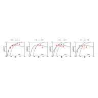
Figure 8.— The total luminosity function for galaxies in the HDF-N (solid black points) and the HDF-S (large crosses) plotted as a function of redshift for the I${}_{814}<27$ sample. The dashed line is the 2dF B-band luminosity function (Norberg et al. 2002), the solid line is the CFRS $z\sim 1$ luminosity function (Lilly et al. 1995) and the dashed line plotted for panels at $z>2$ is the rest-frame B-band Lyman-break galaxy luminosity function (Shapley et al. 2001).

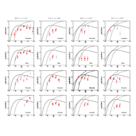
Figure 9.— The luminosity function as function of morphological type and redshift. The points and lines are the same as in Figure 8.

Figure 10.— The luminosity density and luminosity fraction as a function of morphological type and redshift. The upper solid line and open circles shows the total B-band luminosity density in the the HDF-N and HDF-S. The solid line and solid circles show the luminosity density evolution for peculiar galaxies, while the triangles and dashed line and the boxes and dotted lines are the luminosity densities for disks and ellipticals, respectively. The larger open symbols at $z<1$ for the total and morphologically divided luminosity densities are taken from Brinchmann & Ellis (2000).

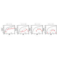
Figure 11.— The total mass function as a function of redshift for the HDF-N (solid black points) and the HDF-S (large crosses) plotted in four different redshift bins for the I${}_{814}<27$ sample. The dashed line shows the $z\sim 0$ mass function from 2dF+2MASS observations (Cole et al. 2001).

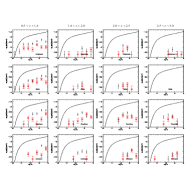
Figure 12.— Mass functions as a function of morphological type. The dashed line is the 2dF+2MASS mass function (Cole et al. 2001). Lines and symbols are the same as in Figure 11.

Figure 13.— The evolution and fraction of stellar mass as a function of morphology out to $z\sim 3$. As in Figure 10, the solid upper line is the total mass density as a function of redshift with the $z\sim 0$ point from the 2MASS data of Cole et al. (2001). The $z\sim 0$ points for the elliptical and disk stellar masses are taken from Fukugita et al. (1998).

Figure 14.— Left panel: The distribution of stellar mass as a function of redshift and morphology. The solid and dashed lines are the values of M^∗ computed by Cole et al. (2001) for Salpeter and Kennicutt initial mass functions, respectively. The long dashed line is the curve above which we are complete, corresponding to a maximally old stellar population. Right panel: the distribution of stellar mass to light ratios (M_∗/L_B) as a function of redshift and morphological type in the HDF fields. The solid line shows the evolution of M_∗/L_B for a single stellar population that is as old as the universe’s age at each redshift.

Figure 15.— The concentration-asymmetry diagram for galaxies in the HDF-N and S divided by redshift. The curved and straight solid lines and the dashed line divide spaces where early, mid, late-type galaxies and mergers are found in the nearby galaxy population (Conselice et al. 2000a; Bershady et al. 2000). Plotted on this diagram are galaxies which are chosen by eye to be ellipticals, disks or peculiars.

Figure 16.— The clumpiness-asymmetry diagram for galaxies in the HDF-N and HDF-S. The solid line is the relationship between $S$ and $A$ found for nearby normal galaxies (Conselice 2003), while the dashed lines are the 3$\sigma$ scatter for this $z\sim 0$ relationship. Galaxies which are too asymmetric for their clumpiness are mergers in the nearby universe.

Figure 17.— The color-asymmetry diagrams for the HDF fields. The solid line is the relationship between these two quantities at $z\sim 0$ (Conselice 2003). The dashed lines are the $z\sim 0$ 3$\sigma$ scatter from this relationship.

References

- (1) Abraham, R.G., van den Bergh, S., Glazebrook, K., Ellis, R.S., Santiago, B.X., Surma, P. & Griffiths, R.E., 1996, ApJS, 107, 1
- (2) Abraham, R.G., Tanvir, N.R., Santiago, B.X., Ellis, R.S., Glazebrook, K., & van den Bergh, S. 1996, MNRAS, 279, 47L
- (3) Baldry, I.K., Glazebrook, K., Brinkmann, J., Ivezic, Z., Lupton, R.H., Nichol, R.C., & Szalay, A.S. 2004, ApJ, 600, 681
- (4) Bell, E.F., McIntosh, D.H., Katz, N., Weinberg, M. 2003, ApJS, 149, 289
- (5) Bershady, M.A., Jangren, J.A., & Conselice, C.J. 2000, AJ, 119, 2645
- (6) Bertin, E., & Arnouts, S. 1996, A&AS, 117, 393
- (7) Blanton, M., et al. 2001, AJ, 121, 2358
- (8) Brinchmann, J., et al. 1998, ApJ, 499, 112
- (9) Brinchmann, J., & Ellis, R.S. 2000, ApJ, 536, 77L
- (10) Bruzual, G., & Charlot, S. 2003, MNRAS, 344, 1000
- (11) Budavári, T., Szalay, A.S., Connolly, A.J., Csabai, I., & Dickinson, M. 2000, AJ, 120, 1588
- (12) Bundy, K. Fukugita, R.S., Ellis, R.S., Kodama, T., & Conselice, C.J. 2004, ApJ, 600, 123L
- (13) Casertano, S., et al. 2000, AJ, 120, 2747
- (14) Chapman, S.C., Windhorst, R., Odewahn, S., Yah, H., Conselice, C. 2003, ApJ, 599, 92
- (15) Cohen, J., Hogg, D.W., Blandford, R., Cowie, L.L., Hu, E., Songaila, A., Shopbell, P., & Richberg, K. 2000, ApJ, 538, 29
- (16) Cole., S. et al. 2001, MNRAS, 326, 255
- (17) Conselice, C.J. 1997, PASP, 109, 1251
- (18) Conselice, C.J., Bershady, M.A., & Jangren, A. 2000a, ApJ, 529, 886
- (19) Conselice, C.J., Bershady, M.A., & Gallagher, J.S. 2000b, A&A, 354, 21L
- (20) Conselice, C.J., Gallagher, J.S., Calzetti, D., Homeier, N., & Kinney, A. 2000c, AJ, 119, 79
- (21) Conselice, C.J., Gallagher, J.S., & Wyse, R.F.G. 2002, AJ, 123, 2246
- (22) Conselice, C.J. 2003, ApJS, 147, 1
- (23) Conselice, C.J., Bershady, M.A., Dickinson, M., & Papovich, C. 2003, AJ, 126, 1183
- (24) Conselice, C.J., Chapman, S.C., Windhorst, R.A. 2003, ApJ, 596, 5L
- (25) Conselice, C.J., et al. 2004, ApJ, 600, L139
- (26) Conselice, C.J., astro-ph/0407463
- (27) Daddi, E., et al. 2004, ApJ, 600, 127L
- (28) de Mello, D.F., Gardner, J.P., Dahlen, T., Conselice, C.J., Grogin, N.A., Koekemoer, A.M. 2004, ApJ, 600, 151L
- (29) de Vaucouleurs, G., de Vaucouleurs, A., Corwin, H. G., Jr., Buta, R. J., Paturel, G., Fouque, P. 1991, “Third Reference Catalogue of Bright Galaxies”, Springer-Verlag
- (30) Dickinson, M., et al. 2000, ApJ, 531, 624
- (31) Dickinson, M., Papovich, C., Ferguson, H.C., Budavári, T. 2003, ApJ, 587, 25
- (32) Driver, S.P., Windhorst, R.A., Ostrander, E.J., Keel, W.C., Griffiths, R.E., Ratnatuna, K.U. 1995, ApJ, 449, 23L
- (33) Drory, N., Bender, R., Feulner, G., Hopp, U., Maraston, C., Snigula, J., & Hill, G.J. 2004, ApJ, 608, 742
- (34) Ellis, R.S. 1997, ARA&A, 35, 389
- (35) Fontanta, A., et al. 2003, ApJ, 594, L9
- (36) Franx, M. et al. 2003, ApJ, 587, 79L
- (37) Frei, Z., 1996, AJ, 111, 174
- (38) Fukugita, M., Shimasaku, K., & Ichikawa, T. 1995, PASP, 107, 945
- (39) Fukugita, M., Hogan, C.J., & Peebles, P.J.E. 1998, ApJ, 503, 518
- (40) Giavalisco, M. et al. 2004, ApJ, 600, L93
- (41) Giavalisco, M., Steidel, C.C., Adelberger, K.L., Dickinson, M.E., Pettini, M., Kellogg, M. 1998, ApJ, 503, 543
- (42) Glazebrook, K., Ellis, R., Santiago, B., & Griffiths, R. 1995, MNRAS, 275, 19L
- (43) Glazebrook, K., et al. 2004, Nature 430, 181
- (44) Graham, A.W., Trujillo, I., & Caon, N. 2001, AJ, 122, 1707
- (45) Hogg, D.W., et al. 2002, AJ, 124, 646
- (46) Kajisawa, M., & Yamada, T. 2001, PASJ, 53, 833
- (47) Kauffmann, G., et al. 2003, MNRAS, 341, 54
- (48) Labbé, I., et al. 2003, AJ, 125, 1107
- (49) Lilly, S.J., Tresse, L., Hammer, F., Crampton, D., LeFevre, O. 1995, ApJ, 455, 108L
- (50) Madau, P., Ferguson, H.C., Dickinson, M., Giavalisco, M., Steidel, C., Fruchter, A. 1996, MNRAS, 283, 1388
- (51) Marzke, R.O., da Costa, L.N., Pellegrini, P.S., Willmer, C.N.A., & Geller, M.J. 1998, ApJ, 503, 617
- (52) Mobasher, B., Jogee, S. Dahlen, T., de Mello, D., Lucas, R.A., Conselice, C.J., Grogin, N.A., & Livio, M. 2004, 600, L146
- (53) Moustakas, L. et al. 2004, ApJ, 600, L131
- (54) Norberg, P., et al. 2002, MNRAS, 332, 827
- (55) Papovich, C., Dickinson, M., & Ferguson, H.C. 2001, ApJ, 559, 620
- (56) Papovich, C. 2002, PhD, Johns Hopkins University
- (57) Papovich, C., Dickinson, M., Giavalisco, M., Conselice, C.J., Ferguson, H.C. 2003, ApJ, 598, 827
- (58) Poggianti, B.M. 1997, A&AS, 122, 399
- (59) Rudnick, G., et al. 2003, ApJ, 599, 84
- (60) Sawicki, M., & Mallen-Ornelas, G. 2003, AJ, 126, 1208
- (61) Schade, D., Lilly, S.J., Crampton, D., Hammer, F., LeFevre, O., Tresse, L. 1995, ApJ, 451, 1L
- (62) Shapley, A.E., Steidel, C.C., Adelberger, K.L., Giavalisco, M., & Pettini, M. 2001, 562, 95
- (63) Somerville, R.S., et al. 2004, ApJ, 600, 135L
- (64) Spergel, D.N., et al. 2003, ApJS, 148, 175
- (65) Stanford, A., et al. 2004, AJ, 127, 131
- (66) Steidel, C.C., Adelberger, K.L., Giavalisco, M., Dickinson, M., & Pettini, M. 1999, ApJ, 519, 1
- (67) Steidel, C.C., Adelberger, K.L., Shapely, A., Pettini, M., Dickinson, M., & Giavalisco, M. 2003, ApJ, 592, 728
- (68) Williams, R.E., et al. 1996, AJ, 112, 1335
- (69) Windhorst, R.A., et al. 2002, ApJS, 143, 113
- (70) Wolf, C., Meisenheimer, K., Rix, H.-W., Borch, A., Dye, S., & Kleinheinrich, M. 2003, A&A, 401, 73
- (71) Yahata, N., Lanzetta, K.M., Chen, H.-W., Fernandez-Soto, A., Pascarelle, S.M., Yahil, A., Puetter, R.C. 2000, ApJ, 538, 493
- (72) van den Bergh, S., Cohen, J.G., Hogg, D.W., & Blandford, R. 2000, AJ, 120, 2190
- (73) van den Bergh, S., Cohen, J.G., & Crabbe, C. 2001, AJ, 122, 611
- (74) van Dokkum, P., et al. 2003, ApJ, 587, 83L