Information bedeutet Horizonterweiterung, und zwar immer auf Kosten der Nestwärme. Sie ist eine Nötigung, anderem, fernem und fremdem Geschick und Geschehen Aufmerksamkeit zu widmen.

Hans-Jürgen Schultz

?chaptername? 1 Introduction

Active galactic nuclei, or AGN, have received considerable attention during the last 40 years. When Maarten Schmidt recognized in 1963 that the quasi-stellar object 3C 273 has a redshift of almost 0.16 (Schmidt 1963), it became immediately clear that there were objects outside our galaxy with tremendous luminosities. Zeldovich (1964), Salpeter (1964) and Lynden-Bell (1969) suggested that extragalactic radio sources were mainly driven by gas accreted into a disc around super-massive black holes, and Blandford & Königl (1979) suggested that the radio emission from AGN is produced by a relativistic outflow of plasma along magnetic field lines. Their model, with numerous modifications, is still thought to be valid, and hence the basic foundations of what we know about AGN today are almost 25 years old.

Like in all branches of astronomy, the progress in AGN science was tightly correlated with technical improvements. Radio astronomy started out with very low angular resolution due to relatively small dishes and long wavelengths. This made $\lambda/D$, governing the resolution of any observing instrument, very poor compared to optical instruments. Almost simultaneously, however, astronomers started to experiment with radio interferometers with progressively longer baselines and finally, to combine interferometric measurements to simulate a larger dish (Ryle & Hewish 1960). This technique is called “aperture synthesis” and was transferred from directly linked, locally distributed antennas to spatially widely separated radio telescopes in the 1970s. What is known as VLBI, or Very Long Baseline Interferometry, today, is a combination of single-dish radio astronomy, interferometry and aperture synthesis, and therefore certainly one of the most advanced technical achievements of the 20th century. Consequently, in 1974, Sir Martin Ryle was awarded the Nobel prize in physics for his contribution.

AGN science and VLBI are tightly interrelated: no other instrument yields the angular resolution necessary to spatially resolve the innermost regions of AGN and details in the jets, and AGN are almost the only objects that are observable with VLBI, with a few exceptions like masers or extremely hot gases. Thus, one cannot live without the other, but the connection has turned out to be very fruitful.

1.1 The AGN Zoo

The first AGN-related phenomena, although not recognized as such, were reported as early as 1908 (Fath 1908) and in the following decades (Slipher 1917, Humason 1932, Mayall 1934), when observers noticed bright emission lines from nuclei of several galaxies, and the first extragalactic jet in M87 was observed (Curtis 1918). The first systematic study of these objects was carried out by Carl Seyfert (Seyfert 1943). He noticed that emission lines from the nuclei of six galaxies were unusually broadened (several $1000\,{\rm km\,s^{-1}}$), but simply stated that this phenomenon was “probably correlated with the physical properties of the nucleus”, without any further interpretation. In the 1950s and 1960s, the first radio sky surveys were completed and catalogues, like the Third Cambridge Catalogue, were published. When interferometric techniques were further developed, all kinds of differences between the AGN turned up, and following ancient habits, astronomers started to classify what they observed. Meanwhile, they have created a colourful collection of mostly phenotypical classes and an equally colourful bunch of acronyms to describe these classes.

1.1.1 The General Picture

?figurename? 1.1: Schematic of AGN (not to scale). Different AGN types are believed to be due to different viewing angles.

The current idea of what AGN are is shown in Fig. 1.1. A supermassive black hole ($M_{\rm\bullet}$ between $10^{6}\,M_{\odot}$ and $10^{9}\,M_{\odot}$) accretes surrounding material that settles in a circumnuclear accretion disc. Some of the material’s potential energy in the gravitational field of the AGN is turned into radiation by viscous friction in the accretion disc, but most of both matter and energy ends up in the black hole. Some of the material is expelled into two jets in opposite directions. Whether the jets are made of an electron-proton or an electron-positron plasma is still controversial, but as the observed radiation is certainly synchrotron radiation, given the high brightness temperatures and degrees of polarization, it must be ionized material circulating in magnetic fields. The jets are not smooth, and in many cases new components are observed as they are ejected from the AGN and travel outwards into the jet direction, and jet bends of any angle are observed. Though not very well determined, around 10 % of the material’s rest mass is turned into energy, the process thus being incredibly efficient compared to hydrogen burning in stars, where only 0.7 % of the hydrogen mass is turned into energy in the production of helium. Thermal gas from the jet surroundings may also be entrained into the jet. The jets can propagate very large distances, e.g. more than 100 kpc in the case of Cygnus A, thus forming the largest physically connected structures in the universe (after cluster galaxies). At distances of less than a parsec, high-density ($10^{8}\,{\rm cm^{-3}}$) gas clouds orbit the AGN and form the broad line region, or BLR. These clouds have speeds of several thousand kilometres per second and hence cause the linewidths observed by Seyfert in 1943. Further out, slower gas clouds constitute the narrow line region, or NLR, with lower densities ($10^{3}\,{\rm cm^{-3}}$) and speeds of only a few hundred kilometres per second. Surrounding the AGN and its constituents in the polar plane is a toroidal agglomeration of material that can deeply hide the AGN and its activity.

After two decades of hassle with AGN phenotypes it became clear in the 1990s that there are basically two separate kinds of AGN classification: each object either is radio loud or radio quiet, and either belongs to the type 1 or 2 AGN. The former classification is based on the ratio of radio luminosity to optical luminosity, $R$, with the dividing line being at around $R=1$ (Kellermann et al. 1989). The latter classification is based on whether the optical emission lines are broad (type 1) or narrow(type 2).

The cause of the bimodality in radio luminosity is still unknown, but several suggestions have been made, involving either “intrinsic” differences in the central engine or “extrinsic” differences in the surrounding medium. Intrinsic differences that have been suggested include (1) systematically lower black hole masses (Laor 2000), (2) lower black hole spins (Wilson & Colbert 1995), (3) a “magnetic switch” that was identified by Meier et al. (1997) during numerical modelling of jets, (4) the production of buoyant plasmons that bubble up through the density gradient of the NLR instead of a collimated relativistic jet (Pedlar et al. 1985, Whittle et al. 1986, Taylor et al. 1989), (5) a large thermal plasma fraction in the jet (Bicknell et al. 1998), or (6) radiative inefficiency (Falcke & Biermann 1995). Extrinsic differences generally invoke the rapid deceleration of initially relativistic jets by collisions in a dense surrounding BLR or interstellar medium (e.g. Norman & Miley 1984). Unfortunately, there are still only very few observational constraints, especially because the radio-weak objects are difficult to observe, and with so many possible causes, the question remains open why they have such low absolute luminosities.

Unlike the difference between radio-loud and radio-quiet objects, the separation into type 1 and 2 AGN is understood as being due to an orientation effect. It depends on whether one can look into the central regions and see the innermost few tenths of a parsec, where the BLR clouds are, or whether the circumnuclear material shadows the BLR, in which case only narrow emission lines from the NLR are observed. Although each individual object has its peculiarities, virtually all AGN belong to one of the radio loud/quiet and type 1/2 classes.

Before going into the details of classification, a brief description is needed of three relativistic effects which are important in the understanding of AGN: relativistic beaming, Doppler boosting and apparent superluminal motion. The former two terms describe a directional anisotropy of synchrotron emission arising from charges moving at large fractions, $\beta$, of the speed of light, $c$, towards the observer. If an object is moving at an angle $\theta$ towards the observer with speed $\beta c$ so that the Lorentz factor, $\gamma$, with

$$\gamma=\frac{1}{\sqrt{1-\beta^{2}}}$$ (1.1)

is $>>1$, and if the object emits an isotropic flux density $S_{0}(\nu)$, then the radiation is confined to a cone with half opening angle $1/\gamma$ (Fig. 1.2) and the observer measures

$$S(\nu)=S(\nu/\delta)\delta^{3}=S_{0}(\nu)\delta^{3-\alpha},$$ (1.2)

where $\alpha$ is the source spectral index defined here as

$$\alpha=\frac{{\rm log}(S_{\nu_{1}}/S_{\nu_{2}})}{{\rm log}(\nu_{1}/\nu_{2})}$$ (1.3)

and $\delta$ is the Doppler factor

$$\delta=\gamma^{-1}(1-\beta\,{\rm cos}\,\theta)^{-1}.$$ (1.4)

Thus, the radiation is not only confined to a smaller cone (beaming) but the observer also measures an increased flux density (Doppler boosting) because the source is moving nearly as fast as its own radiation. Both effects increase the flux density radiated in the forward direction and decrease it in the opposite direction by the same amount, so that even in relatively modest relativistic sources ($\gamma\approx 4$), the jet to counter-jet ratio of flux densities can reach $10^{6}$.

In the same geometric source configuration (small angle between the line of sight and the jet, relativistic speed of jet material), components can be seen moving at speeds exceeding the speed of light. This is a purely geometric effect: because the component is travelling almost as fast as the radiation it emits, the time interval between the emission of two photons appears shortened to us observers, and the apparent transverse speed can therefore exceed $c$.

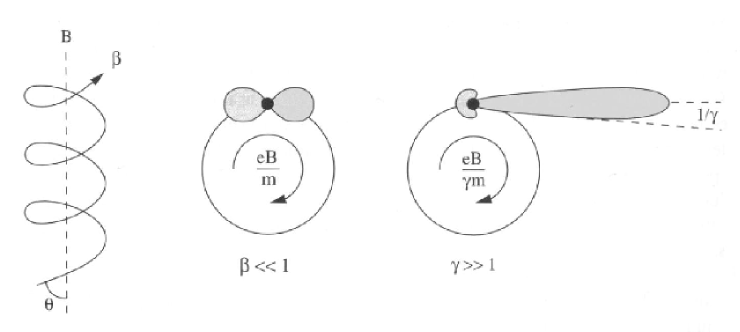
?figurename? 1.2: Sketch of an electron moving in a magnetic field (reproduced from Peacock 1999).

1.1.2 Seyfert Galaxies

Seyfert galaxies belong to the class of radio-quiet AGN. Unlike their powerful siblings, they rarely show clearly defined, linear radio jet structures on pc scales. They are mostly spirals and, although supermassive black holes have been found in some of them (e.g., $3.6\times 10^{7}\,{\rm M_{\odot}}$ in NGC 4258, Miyoshi et al. 1995), their luminosities are only tiny fractions of that observed in quasars and radio galaxies. The sub-division into type 1 and type 2 Seyferts indicates the viewing angle: when the angle between the accretion disc normal and the line of sight is intermediate or small (type 1), one has a direct view onto the BLR, and broad emission lines are visible. If the angle is large, circumnuclear material blocks the direct view onto the central engine and the BLR, and only NLR clouds are seen in the optical. Compelling evidence for this picture comes from galaxies like NGC 1068 which are classified as type 2 Seyferts, but show typical type 1 spectra in polarized light (Antonucci & Miller 1985; Antonucci et al. 1994a). In these cases, the type 1 spectrum is hidden by a foreground absorber, but reflections outside the absorber direct the light into our sight.

1.1.3 Radio Galaxies

Radio galaxies mostly exhibit single-sided, and only rarely two-sided jets on pc scales, but they almost always show two-sided radio emission on kpc scales, mostly in the form of bubble-like, irregularly shaped “radio lobes”. Fifteen percent to 20 % of radio galaxies are radio-loud AGN (e.g., Kellermann et al. 1989). On sub-pc to tens of pc scales, material is transported outwards in collimated jets which exhibit bright knots. On scales of kpc to hundreds of kpc, the jet flow becomes unstable, and either gently fades or abruptly stops in hot spots. Here, huge radio lobes evolve, and the jet material is slowly flowing back into the host galaxy. Because the material in the lobes is no longer relativistic, its emission is isotropic and the visibility of radio lobes is (to zeroth order) independent of the inclination angle. The single-sidedness on pc scales is due to relativistic effects, and only in a few sources where the jets have angles close to $90^{\circ}$ with the line of sight, a double-sided structure on pc scales is seen. Another interpretation of the double-sidedness is that jets are always intrinsically single-sided, and that double-sidedness occurs when the direction of the jet rapidly flips from one side of the accretion disc to the other (e.g., Rudnick & Edgar 1984, Feretti et al. 1993). Similar to Seyfert galaxies, radio galaxies are divided into type 1 and type 2 based on optical appearance and as a result of the same geometric configuration. However, the terms Narrow Line Radio Galaxies (NLRG) and Broad Line Radio Galaxies (BLRG) are also established. A further sub-classification was established for radio galaxies based on their kpc-scale appearance by Fanaroff & Riley (1974). Analysing a sample of 57 radio galaxies and quasars from the 3CR catalogue, they discovered that the relative positions of regions of high and low surface brightness in the lobes of extragalactic radio sources are correlated with their radio luminosity. Fanaroff and Riley divided the sample into two classes using the ratio $R_{\rm FR}$ of the distance between the regions of highest surface brightness on opposite sides of the central galaxy or quasar, to the total extent of the source up to the lowest brightness contour in the map. Sources with $R_{\rm FR}<0.5$ were placed in class I and sources with $R_{\rm FR}>0.5$ in class II. It was found that nearly all sources with luminosity

$$L(178\,{\rm MHz})\leq 2\times 10^{25}\,h_{100}^{-2}\,{\rm W\,Hz^{-1}\,sr^{-1}}$$ (1.5)

were of class I while the brighter sources were nearly all of class II. The boundary between them is not very sharp, and there is some overlap in the luminosities of sources classified as FR-I or FR-II on the basis of their structures. The physical cause of the FR-I/II dichotomy probably lies in the type of flow in the jets. FR-I jets are thought to be subsonic, possibly due to mass entrainment, which makes them amenable to distortions in the interaction with the ambient medium, while the jets in FR-II sources are expected to be highly supersonic, allowing them to travel large distances.

1.1.4 Quasars, BL Lacs, OVVs

The objects in this section all belong to the radio-loud class. If the angle between the jet axis and the line of sight is small, one can see the BLR and the accretion disc directly. Relativistic effects are now dominating the phenotypical properties of the AGN. The jet emission is focused into a narrow cone, and rapid (intra-day) variability might occur. Quasars reveal single-sided pc-scale jets and apparent superluminal motion of knots that travel down the jets. BL Lac objects are highly beamed, they show strong variability from radio to optical wavelengths and they have almost no optical emission lines, neither broad nor narrow. This happens when, at very small inclination angles, the thermal emission from the AGN is superimposed with the optical synchrotron emission from the jet base. At larger inclination angles, the optical synchrotron emission is mostly beamed away from the observer, revealing the underlying thermal emission, and emission lines start to show up. This effect does not occur in the radio regime due to the absence of radio emission lines. The lack of optical emission lines makes a distance determination of BL Lacs difficult. The Optically Violently Variables, or OVVs, are a subclass of the BL Lacs, showing broad emission lines and rapid optical variability.

1.1.5 Compact Symmetric Objects (CSO)

CSOs are double-sided, sub-kpc scale, symmetric radio sources whose spectra frequently have a peak in the GHz regime. Based on size and proper motion measurements, they are commonly regarded as being young ($<10^{4}\,{\rm yr}$) radio galaxies whose jets have not yet drilled their way through the host galaxy’s interstellar medium.

1.2 The Gas Around AGN

The circumnuclear material in AGN is thought to settle in a probably rotationally symmetric body around the black hole. This gas is commonly referred to as the circumnuclear torus, although the toroidal shape has been established in only a few cases. Width, height and radius of this “torus” are not necessarily well constrained and are probably very different from object to object. In any case, however, the torus is expected to shield the central engine from the observer’s view if the inclination angle is right. Observational evidence for tori comes from radio observations of total intensity and H I and molecular absorption and molecular emission, from ${\rm H_{2}O}$ maser observations, from the shape of ionized [O III] and ${\rm H\,\alpha}$+[N II] regions, from X-ray observations and from the detection of thermal emission. A description of the physical properties of the circumnuclear gas can be found in, e.g., Krolik & Lepp (1989).

1.2.1 Radio Absorption Measurements

In those few cases where double-sided pc-scale radio jets are observed, a rather narrow “gap” in the emission across the source is frequently detected towards lower frequencies (e.g., in NGC 1052, Vermeulen et al. 2003, and in NGC 4261, Jones et al. 2001). These gaps are mostly due to free-free absorption, as identified by its characteristic frequency-dependence of the optical depth:

$$\tau_{\nu}\propto\nu^{-2.1}.$$ (1.6)

In these cases, the UV radiation from the AGN ionizes the inner parts of a circumnuclear absorber, and the ionized medium then gives rise to free-free absorption. This situation is seen in, e.g., NGC 1052 (Kameno et al. 2001; Vermeulen et al. 2003), NGC 4261 (Jones et al. 2000, 2001) and Centaurus A (Tingay et al. 2001). A reliable detection of free-free absorption requires flux density measurements at three frequencies at least. If, however, such measurements exist at only two frequencies, the spectral index $\alpha$ can be used to exclude synchrotron self-absorption (SSA). In SSA, the synchrotron radiation produced by the relativistic electrons is absorbed in the source, and if the distribution of the electron energies follows a power law, the spectral index cannot exceed +2.5. Thus, whenever $\alpha>2.5$ is observed at cm wavelengths, the absorption process is most likely free-free absorption (in the cases presented here, the Razin-Tsytovich effect has no effect, see Chapter 3).

H i absorption has been found on sub-pc scales in, e.g., NGC 1052 (Vermeulen et al. (2003)), Cygnus A (Conway & Blanco 1995) and in NGC 4261 (van Langevelde et al. 2000). In the latter, the H i absorption was found no closer than 2.5 pc away from the core, supporting the idea that the material is ionized at smaller distances to the AGN. This was proposed by Gallimore et al. (1999), who detected H i absorption in a number of Seyfert galaxies almost exclusively towards off-core radio components.

A variety of molecular lines is also detected in AGN: NGC 1052 shows OH in absorption and emission (Vermeulen et al. (2003)), in NGC 4261, Jaffe & McNamara (1994) detected CO in absorption and Fuente et al. (2000) found ${\rm CO^{+}}$ absorption in the core of Cygnus A. This list is by no means complete and many other line measurements exist.

1.2.2 Masers

The most compelling evidence for the partly molecular nature of at least parts of the circumnuclear material comes from the detection of ${\rm H_{2}O}$ “megamasers” in the vicinity of AGN. A few prominent examples are NGC 3079 (Henkel et al. 1984, and, more recently, Kondratko 2003), NGC 2639 (Wilson et al. 1995) and NGC 4258 (Miyoshi et al. 1995). In the last case, the velocity distribution of the masers yielded a model-independent measure for the enclosed mass with high accuracy. In NGC 1068, both the alignment and the velocity gradient of the masers found by Gallimore et al. (1996) are oriented perpendicular to the radio jet axis, hence suggesting the presence of a circumnuclear, relatively dense region of material. The physical properties of ${\rm H_{2}O}$ in AGN have been described by Neufeld et al. (1994).

1.2.3 Ionization Cones

In the last 15 years, optical observations of AGN showed cone-shaped regions of line emission (Pogge 1988), frequently in two opposite directions (Storchi-Bergmann et al. 1992; Wilson et al. 1993) and sometimes aligned with linear radio structures (Falcke et al. 1998). The shape of the line emitting regions was immediately interpreted as being due to shadowing by circumnuclear material, i.e., the nuclear UV emission can only escape towards the poles of the torus, where it ionizes the gas.

1.2.4 X-ray Observations

Evidence for circumnuclear absorbers also comes from X-ray observations. Marshall et al. (1993) showed that the X-ray spectrum of NGC 1068 is best modelled as a continuum source seen through Compton scattering. In Cygnus A, Ueno et al. (1994) found evidence for an absorbed power-law spectrum. Seyfert 2 galaxies are mostly heavily absorbed in the X-ray regime, with column densities of the order of $>10^{24}\,{\rm cm^{-2}}$ (Krolik & Begelman 1988).

1.2.5 Thermal Emission

In NGC 1068, Gallimore et al. (1997) have discovered a region of flat-spectrum radio continuum emission with brightness temperatures too low to be due to self-absorbed synchrotron emission. The shape and orientation of the region is suggestive of a circumnuclear disc or torus, and they conclude that the emission is either due to unseen self-absorbed synchrotron emission that is reflected by a torus into the line of sight or free-free emission from the torus itself.

1.3 Feeding Gas Into the AGN

1.3.1 Magnetic Fields

A lot of material is seen in the vicinity of AGN, but how is the material moved closer to and into the black hole and into the jets? Shlosman et al. (1989) suggested that a stellar bar in a galaxy sweeps gas into the central few hundred pc. The gas forms a disc which also develops a bar potential and funnels the gas further in to scales of a hundred parsecs. Processes that transport the gas further in to parsec scales are largely unknown, and no theory exists that could be tested by observations. To move gas into smaller radius orbits requires a mechanism to shed angular momentum, and the candidates are viscosity and magnetic fields. Viscosity, responsible for angular momentum transport in the innermost regions of AGN, would form the gas into a disc, which is not generally observed. Only in few objects have such discs with diameters of $\leavevmode\nobreak\ \sim 100\,{\rm pc}$ been found (e.g., in NGC 4261, Jaffe et al. 1996; Ferrarese et al. 1996 and in Mrk 231, Klöckner et al. 2003), but the role that the discs in these objects play in gas transport is unclear.

Magnetic fields, on the other hand, play an essential role in models of tori, accretion discs and jet formation in the central parsec and sub-parsec scale regions (e.g., Koide et al. 2000; Meier et al. 2001; Krolik & Begelman 1988). The basic idea is that the accretion disc is threaded with magnetic fields, and that differential rotation of the disc twists the fields to a spiral structure, which applies a breaking torque on the inner disc and accelerates material in the outer disc, thus transporting angular momentum outwards.

The origin of the required magnetic fields is not clear. They are probably frozen into the accreted material on scales of $>10\,{\rm pc}$, although parts of the field may be lost in reconnection. Dynamo processes in the disc can also produce magnetic fields (e.g., von Rekowski et al. 2003) which participate in the generation of an outflow, but the details are not well known. Estimates of magnetic field strengths in AGN and their surroundings mainly come from equipartition arguments, assuming that the energy in particles equals that in magnetic fields. Whether this assumption is justified or not is not known, and so equipartition arguments are unsatisfactory.

Magnetic fields are routinely observed on the largest scales in galaxies and are modelled on the smallest, but are largely unknown on intermediate scales of a few parsecs to several tens of parsecs. As they are probably involved in the transport of gas into the AGN, their strength and orientation is of considerable interest.

1.3.2 Faraday Rotation and Free-Free Absorption

One way to measure magnetic field strengths is by means of Faraday rotation. When an electromagnetic wave travels through an ionized medium that is interspersed with a magnetic field with a component parallel to the direction in which the wave is travelling, then the plane of polarization of the wave is rotated. The amount of Faraday rotation cannot be measured directly because the intrinsic position angle of the polarization is not known and the rotation has ambiguities of $\pi$. Instead, one exploits the frequency dependence of the Faraday rotation, and the change of the effect with frequency yields the constant of proportionality, the rotation measure $RM$.

The physics behind this effect is the birefringence of the magnetized plasma. A linearly polarized beam of radiation with electric vector position angle $\theta$ can be considered as the superposition of two circularly polarized waves with equal amplitudes but opposite senses of rotation. The circular polarizations have different indices of refraction in the plasma which causes one polarization to be retarded with respect to the other, and the plane of linear polarization, composed of the two circular polarizations, rotates.

Faraday rotation is of particular importance in this thesis so we give a brief derivation of the formula here, following Kraus & Carver 1973, p. 737f.

In a magnetized plasma, where the magnetic field is parallel to the direction of propagation of the waves, the phase constants $\beta^{+}$ and $\beta^{-}$ of the two waves are given by

$$\beta^{\pm}=\omega\sqrt{\mu_{0}(\epsilon_{11}\pm\epsilon_{12})},$$ (1.7)

where $\omega$ is the angular frequency of the wave, $\mu_{0}$ is the vacuum permeability, and $\epsilon_{11}$ and $\epsilon_{11}$ are elements of the permittivity tensor $\overline{\epsilon}$, with

$$\begin{split}\epsilon_{11}&=\left(1+\frac{\omega_{0}^{2}}{\omega_{\rm g}^{2}-\omega^{2}}\right)\epsilon_{0}\\ \epsilon_{12}&=\frac{-i\omega_{0}^{2}\omega_{\rm g}\epsilon_{0}}{\omega(\omega_{\rm g}^{2}-\omega^{2})}\\ \end{split}$$ (1.8)

Here, $\omega_{0}=e\sqrt{n_{\rm e}/\epsilon_{0}m}$ denotes the angular plasma frequency ($e$ is the particle charge in C, $n_{\rm e}$ the particle density in ${\rm m^{-3}}$ and $m$ the particle mass in kg), $\omega_{\rm g}=(e/m)B$ the angular gyrofrequency and $\epsilon_{0}$ the vacuum permittivity. Travelling a distance $dl$ through the plasma changes $\theta$ by

$$d\theta=\frac{\beta^{-}-\beta^{+}}{2}dl.$$ (1.9)

Inserting the expressions for $\omega_{0}$ and $\omega_{\rm g}$ into Eq. 1.7 and integrating over the line of sight then yields

$$\begin{split}\theta&=\lambda^{2}\times\frac{e^{3}}{8\pi^{2}c^{3}\epsilon_{0}m^{2}}\int_{0}^{L}n_{\rm e}\,B_{\parallel}\,dl\\ &=\lambda^{2}\times 2.63\times 10^{-13}\int_{0}^{L}n_{\rm e}\,B_{\parallel}\,dl\\ &=\lambda^{2}\times RM,\end{split}$$ (1.10)

where $\lambda$ is the wavelength in m, $e$ is the elementary charge in C, $c$ is the speed of light in ${\rm m\,s^{-1}}$, $\epsilon_{0}$ is the vacuum permittivity in ${\rm F\,m^{-1}}$, $m$ is the electron mass in kg, $n_{\rm e}$ is the electron density in ${\rm m^{-3}}$, $B_{\parallel}$ is the line-of-sight component of the magnetic flux density in T, and $l$ is the path length in m.

Observations of Faraday rotation yield a measure of the integral of the product $n_{\rm e}\,B_{\parallel}$. To separate the magnetic field from the electron density requires an independent measurement of the electron density and the path length through the ionized gas.

Ionized gases also produce free-free absorption which causes an exponential decrease of intensity with path length through the absorber. The spectral energy distribution of synchrotron radiation which is absorbed by free-free absorption, is given by

$$S_{\nu}=S_{0}\,\nu^{\alpha_{0}}\times\exp(-\tau_{\nu}^{\rm ff}),$$ (1.11)

where

$$\tau_{\nu}^{\rm ff}=8.24\times 10^{-2}\,T^{-1.35}\,\nu^{-2.1}\,\int{N_{+}N_{-}ds}$$ (1.12)

(e.g., Osterbrock 1989, eq. 4.32). Here, $S_{\nu}$ is the observed flux density in mJy, $S_{0}$ is the intrinsic flux density (before the radiation passes the absorber) in mJy, $\nu$ is the observing frequency in GHz, $\alpha_{0}$ is the dimensionless intrinsic spectral index, $T$ is the gas temperature in K, $N_{+}$ and $N_{-}$ are the number densities of positive and negative charges, respectively, in ${\rm cm^{-3}}$, and $s$ is the path length in pc.

Faraday rotation depends linearly on the electron density, $n_{\rm e}$, whereas the optical depth in free-free absorption goes as $n_{\rm e}^{2}$ (assuming $N_{+}=N_{-}=n_{\rm e}$). An analysis of the frequency-dependence of $\tau_{\nu}^{\rm ff}$, together with a diameter measurement of the absorber from VLBI images, yields $n_{\rm e}$. Putting $n_{\rm e}$ and the diameter into Eq. 1.10 then allows one to solve for the magnetic field strength, $B_{\parallel}$.

1.3.3 Jet Collimation

As was mentioned in the section §1.3.1, models exist for the innermost regions of AGN where the jets are launched and collimated. Some possible mechanisms for the acceleration of jets are the “magnetic slingshot” model (Blandford & Payne 1982), through the extraction of Poynting flux from the black hole, the so-called Blandford-Znajek mechanism (Blandford & Znajek 1977), or by radiation or thermal pressure (Odell 1981; Livio 1999).

Unfortunately, although today’s radio interferometers routinely yield angular resolutions of 0.1 mas, these regions are still not resolved, except for a few nearby objects with high black hole masses, like M87 (Junor et al. 1999). Jet collimation is expected to happen on scales of 10 to 1000 Schwarzschild radii ($R_{\rm s}$), and in a moderately distant radio galaxy with redshift $z=0.1$ and a typical black hole with $10^{8}\,M_{\odot}$, these scales are still factors of 20 to 2000 smaller than the synthesized beam. Hence, only little observational evidence exists so far to constrain jet formation models. In a few nearby AGN, however, the highest resolution VLBI observations at 86 GHz can in principle resolve scales of $<1000\,R_{\rm s}$. These observations are challenging because most nearby sources are weak at high frequencies and the antenna sensitivities decrease, and most attempts to detect the targets have failed.

1.4 The Aim of This Thesis

Nearby AGN provide unique opportunities to study the circumnuclear environments of supermassive black holes. VLBI observations have long been concentrated on the brightest, but unfortunately more distant objects, yielding rather low linear resolutions of more than one parsec. In this thesis, I present VLBI observations primarily of nearby objects, yielding some of the highest linear resolution images ever made. The goal was to investigate the distribution of gas and magnetic fields in those objects, and to probe the jet collimation region of a nearby radio galaxy with highest linear resolution. This required the development of fast frequency switching for phase calibration of 86 GHz VLBI observations of weak sources.

1.4.1 Polarimetric Observations of Six Nearby AGN

Six nearby AGN were selected because they show good evidence for circumnuclear free-free absorbers that shadow the radiation of the AGN. If such absorbers are interspersed with magnetic fields and the radio emission from the AGN is polarized, Faraday rotation is expected to occur. A joint analysis of the free-free absorption and Faraday rotation then allows one to determine the magnetic field strength in the absorber and so yields a measurement of a quantity which is difficult to determine by other means. I present the results of pilot VLBI observations that were made to look for polarized emission before making time-consuming Faraday rotation measurements.

1.4.2 Case Study of NGC 3079

In addition to the polarimetric observations of NGC 3079, I present an analysis of multi-epoch, multi-frequency observations of this nearby Seyfert 2 galaxy to investigate the nature and origin of the radio emission. Furthermore, I present a statistical analysis of VLBI observations of Seyfert galaxies reported in the literature to compare NGC 3079 to other Seyferts and to compare Seyferts to radio-loud objects to investigate the difference between powerful and weak AGN.

1.4.3 Phase Calibration Strategies at 86 GHz

We have explored the feasibility of a new phase calibration strategy for VLBI observations, in which one cycles between a lower reference frequency, at which the source is strong enough for self calibration, and the target frequency. The phase solutions from the reference frequency are scaled by the frequency ratio and interpolated onto the target frequency scans to remove the atmospheric phase fluctuations. The result is a phase-referenced image at the target frequency, and indefinitely long coherent integrations can be made on sources that are too weak for self-calibration. The primary use of the technique is to image nearby, weak AGN at 86 GHz to obtain highest linear resolutions. Using data from a pilot project, we have improved the observing and data calibration strategy to a ready-for-use level, and we have obtained the first detection of NGC 4261 which could not be imaged previously at 86 GHz because it is too weak.

?chaptername? 2 Special VLBI Techniques

Very Long Baseline Interferometry, or VLBI, has become a standard observing technique in the radio astronomy community during the last 20 years. Although frequently referred to as “experiments”, VLBI observations have left the experimental stage, and especially observations with the U.S. 10-element Very Long Baseline Array, or VLBA, are relatively easy to prepare and analyse, and now the first automated data calibration methods exist (Sjouwerman et al. 2003). A good description of VLBI principles and the data calibration steps required has recently been given by Klare (2003), and details can be found in, e.g., Thompson et al. (1986). I therefore will not go into the details.

There are, however, non-standard VLBI observations that require special observing procedures and/or data calibration steps. Two of these techniques, phase-referencing and polarimetry, have been used to gather data for this thesis and therefore are described in detail. Furthermore, a short section is dedicated to a description of ionospheric phase noise in phase referencing and how it can be calibrated.

2.1 Phase Referencing

In VLBI, the true visibility phase is altered by errors from numerous sources. They can be divided into geometric, instrumental and atmospheric errors. Geometric errors arise from inaccurate antenna positions, motion of antennas with tectonic plate motion, tidal effects, ocean loading and space curvature due to the mass of the sun and the planets close to the targeted position. Instrumental errors include clock drifts, changes in antenna geometry due to gravity forces, cable length changes, and electronic phase errors due to temperature variations. Most of these errors are sufficiently well known or are measured continuously and are accounted for in the correlator model of the array. Atmospheric and ionospheric phase noise, however, is difficult to predict and is therefore the largest source of error in VLBI observations. The following description of the effect of atmospheric and ionospheric phase noise on VLBI observations closely follows Beasley & Conway (1995).

2.1.1 Tropospheric Phase Noise

At cm wavelengths, the largest source of error in VLBI observations comes from fluctuations of the tropospheric water vapour content along the line of sight of the telescopes. Changes in the water vapour content cause phase changes of the observed visibilities and thus limit the atmospheric coherence time. This is the time over which data can be coherently averaged, and is taken to be the average time it takes for the phase to undergo a change by one radian ($\sim 57^{\circ}$).

The tropospheric excess delay, i.e., the additional time it takes for the waves to travel through the atmosphere compared to vacuum, can be divided into two components, the dry troposphere and the wet troposphere. This means that the mixture of air and water vapour would have the same effect on the visibility phases as a layer of dry air and a layer of water vapour, both of thicknesses equivalent to the tropospheric content of air and water vapour, respectively. The zenith excess delay due to the dry troposphere, $l_{\rm z}$, can be modelled quite accurately using measurements of pressure and antenna latitude and altitude (Davis et al. 1985):

$$l_{\rm z}=\frac{0.228\,{\rm m/mbar}\,P_{0}}{1-0.00266\cos(2\lambda)-0.00028\,{\rm km^{-1}}h}.$$ (2.1)

Here, $l_{\rm z}$ is the zenith excess path length in cm, $P_{0}$ is the the total pressure at the surface in mb and $h$ is the altitude of the antenna above the geoid in km. With this equation, the dry troposphere, contributing around 2.3 m, can be modelled to an accuracy of $\approx 0.5\,{\rm mm}$. The equation can be extended to include the tropospheric water vapour, yielding the Saastamoinen model (Rönnäng 1989)

$$l_{\rm z}=\frac{0.228\,{\rm m/mbar}\left[P_{0}+P_{\rm w}\left(\frac{1255}{T}+0.05\right)\right]}{1-0.00266\cos(2\lambda)-0.00028\,{\rm km^{-1}}h}.$$ (2.2)

Here, $P_{\rm w}$ is partial pressure of water vapour and $T$ is the temperature in K. However, the effects of the wet troposphere are much more difficult to describe because the water vapour is not well mixed with the dry air, and turbulence makes the delay due to the wet troposphere highly variable. In general, tropospheric water vapour contributes up to 0.3 m of excess path delay, but to determine the exact value requires precise measurements of the water vapour in front of each telescope. Water vapour radiometers therefore have become increasingly popular, especially at radio telescopes operating at mm wavelength. The new Effelsberg Water Vapour Radiometer (Roy et al. 2003) is now able to measure the delay to an accuracy of 0.12 mm ($1\,\sigma$), corresponding to, e.g., $2.2^{\circ}$ at 15.4 GHz. Further improvements will shortly increase the accuracy to about 0.04 mm and hence allow one to use the water vapour radiometer to calibrate VLBI data at frequencies of up to 86 GHz.

The path length through the atmosphere scales as $\sin^{-1}(\beta$), where $\beta$ is the antenna elevation. Thus, the amount of troposphere along the line of sight has doubled at an elevation of $30^{\circ}$, and has increased to five times its zenith value at $12^{\circ}$ elevation. As a consequence, the phase noise dramatically increases towards low antenna elevations. At frequencies above $\sim 5\,{\rm GHz}$, tropospheric phase noise is the dominant source of error in VLBI observations.

2.1.2 Ionospheric Phase Noise

The ionosphere is a region of free electrons and protons at altitudes of 60 km to 10000 km above the earth’s surface. It adds phase and group delays to the waves and causes Faraday rotation of linearly polarized waves. The excess zenith path in m is (Thompson et al. 1986, eq. 13.128)

$$l_{0}\approx-\frac{40.3\,{\rm Hz^{2}\,m^{3}}}{\nu^{2}}{\rm TEC},$$ (2.3)

where $\nu$ is the frequency in Hz and TEC is the vertical total electron content in ${\rm m^{-2}}$. The TEC changes on various timescales. Long-term variations are caused predominantly by changing solar radiation (solar cycle, seasonal and diurnal variations), but short-term variations are mostly caused by atmospheric gravity waves through the upper atmosphere, oscillations of air caused by buoyancy and gravity. The biggest effect on radio observations are medium-scale travelling ionospheric disturbances (MSTIDs) with horizontal speeds of $100\,{\rm m\,s^{-1}}$ to $300\,{\rm m\,s^{-1}}$, periods of 10 min to 60 min and wavelengths of several hundred km. The ionosphere introduces a delay that scales as $\nu^{-2}$, whilst the phase scales as $\nu^{-1}$, and this contribution is the dominant source of phase error in VLBI observations at frequencies below $\sim 5\,{\rm GHz}$. Ionospheric Faraday rotation is negligible at cm wavelengths, with a maximum of 15 turns of the electric vector position angle at 100 MHz (Evans & Hagfors 1968) and hence at most 9 turns, 3 turns and 1 turn of phase at 1.7 GHz, 5.0 GHz and 15.4 GHz, respectively.

2.1.3 Phase Referencing

In standard VLBI observations at cm wavelengths, the so-called phase self-calibration is used to solve for phase errors that cannot be accounted for by the correlator model and mostly are tropospheric. Starting with a point source model in the field centre, and refining the model iteratively, correction phases are derived that make the visibility phases compliant with the model. This procedure is known as self-calibration, or hybrid mapping (Cornwell & Wilkinson 1981). But in two cases, this procedure does either not work or is not desirable. In the first case, the target source is weak and cannot be detected reliably within the atmospheric coherence time. As an illustration, in a typical 15 GHz VLBA experiment with ten stations in moderate weather, the coherence time is 60 s and the $7\,\sigma$ detection limit follows to 21 mJy, and weaker sources cannot be detected (a detailed calculation of sensitivity limits is given in Chapter 6). In the second case, one is interested in absolute astrometry of the target source. A priori phase self-calibration destroys that information because the visibility phases are initially adjusted to fit a point source at a position provided by the observer. Literally, one can “move around” the source in the field of view and one is always able to properly adjust the visibility phases. Phase-referencing solves both of these problems.

In brief, phase referencing uses interleaved, short observations (“scans”) of a nearby calibrator to measure the tropospheric phase noise which is subtracted from the target source visibilities. It works only if the interval between two calibrator scans is shorter than the atmospheric coherence time and the calibrator structure is well known. The first demonstration of this technique was published by Alef (1988) (a similar approach had already been proven to work by Marcaide & Shapiro 1984, but in their case, the calibrator and target were in the telescope primary beams, and no source switching was needed).

Consider an observing run in which each target source scan of several minutes is sandwiched between short scans on a nearby calibrator. Let us further assume that all a priori calibration information has been applied, i.e., the amplitudes are calibrated and the bandpass shape and instrumental delay and phase offsets are corrected for. The measured visibility phases can then be described with

$$\begin{split}\phi_{\rm cal}(t_{1})&=\phi_{\rm c}(t_{1})+\phi_{\rm ins}^{\rm c}(t_{1})+\phi_{\rm pos}^{\rm c}(t_{1})+\phi_{\rm ant}^{\rm c}(t_{1})+\phi_{\rm atm}^{\rm c}(t_{1})+\phi_{\rm ion}^{\rm c}(t_{1})\\ \phi_{\rm tar}(t_{2})&=\phi_{\rm t}(t_{2})+\phi_{\rm ins}^{\rm t}(t_{2})+\phi_{\rm pos}^{\rm t}(t_{2})+\phi_{\rm ant}^{\rm t}(t_{2})+\phi_{\rm atm}^{\rm t}(t_{2})+\phi_{\rm ion}^{\rm t}(t_{2})\\ \phi_{\rm cal}(t_{3})&=\phi_{\rm c}(t_{3})+\phi_{\rm ins}^{\rm c}(t_{3})+\phi_{\rm pos}^{\rm c}(t_{3})+\phi_{\rm ant}^{\rm c}(t_{3})+\phi_{\rm atm}^{\rm c}(t_{3})+\phi_{\rm ion}^{\rm c}(t_{3}).\\ \end{split}$$ (2.4)

$\phi_{\rm c}$ and $\phi_{\rm t}$ are the true visibility phases on the calibrator and the target source, $\phi_{\rm ins}$ is the residual instrumental phase error due to clock drifts and other electronics, $\phi_{\rm pos}$ and $\phi_{\rm ant}$ are geometric errors arising from source and antenna position errors, and $\phi_{\rm atm}$ and $\phi_{\rm ion}$ are tropospheric and ionospheric phase noise contributions. Using self-calibration, the measured visibility phase is decomposed into the source structure phase and the difference in antenna-based phase errors at $t_{1}$ and $t_{3}$, and interpolation yields the calibrator visibilities at $t_{2}$:

$$\tilde{\phi}_{\rm cal}(t_{2})=\tilde{\phi}_{\rm c}(t_{2})+\tilde{\phi}_{\rm ins}^{\rm c}(t_{2})+\tilde{\phi}_{\rm pos}^{\rm c}(t_{2})+\tilde{\phi}_{\rm ant}^{\rm c}(t_{2})+\tilde{\phi}_{\rm atm}^{\rm c}(t_{2})+\tilde{\phi}_{\rm ion}^{\rm c}(t_{2})\\$$ (2.5)

(a tilde denotes interpolated values). Subtracting the interpolated calibrator visibility phases from the observed target visibility phases at time $t_{2}$ gives

$$\begin{split}\phi_{\rm tar}-\tilde{\phi}_{\rm cal}&=(\phi_{\rm t}-\tilde{\phi_{\rm c}})+(\phi_{\rm ins}^{\rm t}-\tilde{\phi}_{\rm ins}^{\rm c})+(\phi_{\rm pos}^{\rm t}-\tilde{\phi}_{\rm pos}^{\rm c})\\ &+(\phi_{\rm ant}^{\rm t}-\tilde{\phi}_{\rm ant}^{\rm c})+(\phi_{\rm atm}^{\rm t}-\tilde{\phi}_{\rm atm}^{\rm c})+(\phi_{\rm ion}^{\rm t}-\tilde{\phi}_{\rm ion}^{\rm c}).\\ \end{split}$$ (2.6)

In this equation, most terms are zero. Residual instrumental errors vary slower than the lag between the calibrator and target source scan, and therefore $\phi_{\rm ins}^{\rm t}-\tilde{\phi}_{\rm ins}^{\rm c}=0$. Atmospheric and ionospheric noise will also be the same in adjacent scans if the separation between calibrator and target is less than a few degrees and the lines of sight pass through the same isoplanatic patch, the region across which tropospheric and ionospheric contributions are constant. This yields $\phi_{\rm atm}^{\rm t}-\tilde{\phi}_{\rm atm}^{\rm c}=0$ and $\phi_{\rm ion}^{\rm t}-\tilde{\phi}_{\rm ion}^{\rm c}=0$. Antenna position errors have the same effect on both the calibrator and the target if their separation on the sky is small, and hence $\phi_{\rm ant}^{\rm t}-\tilde{\phi}_{\rm ant}^{\rm c}=0$. The calibrator visibility phases change slowly, and hence $\tilde{\phi}_{\rm cal}=\phi_{\rm c}$. Also, when using either a compact calibrator or a good calibrator model in phase self-calibration, the phase errors derived from phase self-calibration are those of a point source, and hence $\tilde{\phi_{\rm c}}=0$. This yields

$$\phi_{\rm tar}-\tilde{\phi}_{\rm cal}=\phi_{\rm t}+(\phi_{\rm pos}^{\rm t}-\tilde{\phi}_{\rm pos}^{\rm c})+\phi_{\rm int},$$ (2.7)

in which $\phi_{\rm int}$ denotes interpolation errors. This equation expresses that after interpolation, the difference between the calibrator and the target source phases is the target source structural phases plus the position error. Hence, phase-referencing not only allows one to calibrate the visibility phases, but also to precisely measure the target source position with respect to the calibrator position.

In general, the ionospheric phase component can be calibrated in self-calibration, together with the tropospheric component. But especially at low elevations and frequencies below 5 GHz, the assumption that $\phi_{\rm ion}^{\rm t}-\tilde{\phi}_{\rm ion}^{\rm c}=0$ is no longer valid, and a correction has to be applied. One approach to correct for the ionospheric delays is to use TEC models derived from GPS data. They are provided by several working groups, yielding global TEC maps every two hours, and giving the TEC on a grid with $2.5^{\circ}$ spacings in latitude and $5^{\circ}$ spacings in longitude. From this grid, the TEC at each antenna can be interpolated. The error in these maps, however, can be quite high, up to 20 % when the TEC is as high as a few tens of TEC units (1 TECU=$10^{16}\,{\rm e^{-}\,m^{-2}}$), and up to 50 % or higher when the TEC is of the order of a few TEC units. Details on how the TEC is derived from GPS data are discussed by Ros et al. (2000), and a set of tests is described in Walker & Chatterjee (2000).

2.2 Polarimetry

Measuring the linear or circular polarization of radio waves is a relatively young technique in VLBI. The first polarization-sensitive VLBI observation of an AGN jet was published by Cotton et al. (1984) (unfortunately, their 3C 454.3 image was rotated by $180^{\circ}$ because they had mistaken the phase signs). But VLBI polarimetry has become increasingly popular, leading to extensive surveys in the last few years (e.g., Zavala & Taylor 2003; Pollack et al. 2003). This section describes technical details and calibration of polarization-sensitive VLBI observations.

2.2.1 Stokes Parameters

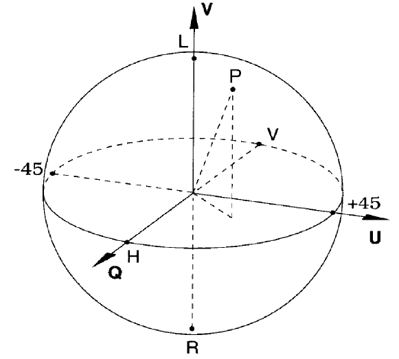
?figurename? 2.1: The Poincaré sphere, reproduced from Scott et al. (2001).

The polarization of any source can be described by means of the Stokes parameters $I$, $Q$, $U$ and $V$. $I$ denotes the total intensity of the source, $Q$ and $U$ the fractions of linear polarization perpendicular to the propagation of the wave and in directions that enclose angles of $45^{\circ}$, and $V$ denotes the fraction of circular polarization. A convenient way to look at this is the Poincaré sphere (Fig. 2.1). Consider a Cartesian coordinate system in which $Q$ is on the $x$ axis, $U$ is on the $y$ axis and $V$ is on the $z$ axis. The radius of the sphere is the degree of polarization,

$$I_{\rm p}=\sqrt{Q^{2}+U^{2}+V^{2}},$$ (2.8)

and the points on the sphere represent the different states of polarization. The intersection points of the $Q$, $U$ and $V$ axes with the sphere represent the following states of polarization, respectively: linear, horizontal ($+Q$), linear, vertical ($-Q$), linear, $+45^{\circ}$ ($+U$), linear $-45^{\circ}$ ($-U$), circular, left-handed ($+V$) and circular, right-handed ($-V$). In general, the polarization is a combination of all three parameters, and the polarization is elliptical.

2.2.2 Interferometer Response to a Polarized Signal

Determination of an extended source’s polarization characteristics requires measuring the Stokes parameters over the source region. An interferometer with coordinates $(u,v)$ in the plane perpendicular to the line of sight measures the Fourier transform of the sky brightness distribution, given in angular coordinates $(\zeta,\eta)$. Similar to the Fourier transform of the total intensity brightness distribution, $I$, the interferometer response to the sky distribution of the other Stokes parameters, $Q$, $U$ and $V$ can be defined:

$$\begin{split}\mathscr{I}(u,v)&=\int\int I(\zeta,\eta)e^{-j2\pi(\zeta u+\eta v)}d\zeta d\eta\\ \mathscr{Q}(u,v)&=\int\int Q(\zeta,\eta)e^{-j2\pi(\zeta u+\eta v)}d\zeta d\eta\\ \mathscr{U}(u,v)&=\int\int U(\zeta,\eta)e^{-j2\pi(\zeta u+\eta v)}d\zeta d\eta\\ \mathscr{V}(u,v)&=\int\int V(\zeta,\eta)e^{-j2\pi(\zeta u+\eta v)}d\zeta d\eta.\\ \end{split}$$ (2.9)

Starting with the interferometer response to a point source, I now describe how the quantities $I$, $Q$, $U$ and $V$ are restored from the visibility measurements. I then describe the calibration of polarization-sensitive interferometer data. The polarization calibration procedure used in this thesis was developed by Leppänen et al. (1995). I follow their notation to explain the interferometer response and the correlation to the Stokes parameters; the full derivation can be found in Leppänen (1995).

Response to a Point Source

The voltages $A$ present at an antenna output can be described by

$$\begin{split}A^{R}&=g^{R}(E^{R}e^{-j\alpha}+E^{L}D^{R}e^{j\alpha})\\ A^{L}&=g^{L}(E^{L}e^{j\alpha}+E^{R}D^{L}e^{-j\alpha}).\\ \end{split}$$ (2.10)

Here, the $g$’s are complex quantities proportional to the antenna gains, $E$’s are the RCP and LCP parts of the electric field, respectively, $D$’s are the complex leakage of power from one polarization into the other, and $e^{\pm j\alpha}$ describe the rotation of the wave with respect to the feed horns due to the parallactic angle of the source, $\alpha$. These terms are commonly referred to as $D$-terms. Because virtually all sources exhibit fractional polarizations that are of the same order as the $D$-terms on the scales probed with VLBI, the significance of the detection of polarized emission depends critically on the $D$-terms being properly calibrated. All quantities, except for $D$, are functions of time.

The cross-correlation function, $\rho$, between two antennas is given by

$$\rho^{pq}_{mn}(\tau)=\langle A^{p}_{m}(t)A^{q}_{n}(t-\tau)\rangle.$$ (2.11)

This equation expresses an average of the multiplication of the antenna voltages, $A$, from two antennas, $m$ and $n$, with a certain delay, $\tau$. The indices $p$ and $q$ represent either LCP or RCP, yielding four possible combinations for each baseline. The functions $A$ are real, and hence their cross-correlation is equal to their convolution. One gets the cross-power spectrum, $r(\omega)$, by Fourier-transforming Eq. 2.11. Applying the convolution theorem then yields

$$r^{pq}_{mn}(\omega)=\mathscr{A}^{p}_{m}(\omega)\mathscr{A}^{q*}_{n}(\omega),$$ (2.12)

where the $\mathscr{A}(\omega)$ are the Fourier transforms of the terms in Eq. LABEL:eq:antenna-output. Eq. 2.12 is valid for any antenna pair because we still assume a point source in the field centre, and the interferometer amplitude therefore is independent of baseline length and orientation.

When Eq. LABEL:eq:antenna-output is inserted into Eq. 2.11 before Fourier transformation, Eq. 2.12 contains the terms $E^{R}E^{R*}$, $E^{L}E^{L*}$ $E^{R}E^{L*}$ $E^{L}E^{R*}$, which we denote by $RR$, $LL$, $RL$ and $LR$, and their Fourier transforms by $\mathscr{RR}$, $\mathscr{LL}$, $\mathscr{RL}$ and $\mathscr{LR}$. The four cross-power spectra then take on the form

$$\begin{split}r^{RR}_{mn}=g^{R}_{m}g^{R*}_{n}&[e^{-j(\alpha_{m}-\alpha_{n})}\times\mathscr{RR}+D^{R}_{m}e^{j(\alpha_{m}+\alpha_{n})}\times\mathscr{LR}\\ &+D^{R*}_{n}e^{-j(\alpha_{m}+\alpha_{n})}\times\mathscr{RL}+D^{R}_{m}D^{R*}_{n}e^{j(\alpha_{m}-\alpha_{n})}\times\mathscr{LL}]\\ r^{LL}_{mn}=g^{L}_{m}g^{L*}_{n}&[e^{j(\alpha_{m}-\alpha_{n})}\times\mathscr{LL}+D^{L}_{m}e^{-j(\alpha_{m}+\alpha_{n})}\times\mathscr{RL}\\ &+D^{L*}_{n}e^{j(\alpha_{m}+\alpha_{n})}\times\mathscr{LR}+D^{L}_{m}D^{L*}_{n}e^{-j(\alpha_{m}-\alpha_{n})}\times\mathscr{RR}]\\ r^{RL}_{mn}=g^{R}_{m}g^{L*}_{n}&[e^{-j(\alpha_{m}+\alpha_{n})}\times\mathscr{RL}+D^{R}_{m}e^{j(\alpha_{m}-\alpha_{n})}\times\mathscr{LL}\\ &+D^{L*}_{n}e^{-j(\alpha_{m}-\alpha_{n})}\times\mathscr{RR}+D^{R}_{m}D^{L*}_{n}e^{j(\alpha_{m}+\alpha_{n})}\times\mathscr{LR}]\\ r^{LR}_{mn}=g^{L}_{m}g^{R*}_{n}&[e^{j(\alpha_{m}+\alpha_{n})}\times\mathscr{LR}+D^{L}_{m}e^{-j(\alpha_{m}-\alpha_{n})}\times\mathscr{RR}\\ &+D^{R*}_{n}e^{j(\alpha_{m}-\alpha_{n})}\times\mathscr{LL}+D^{L}_{m}D^{R*}_{n}e^{-j(\alpha_{m}+\alpha_{n})}\times\mathscr{RL}].\\ \end{split}$$ (2.13)

This particular representation of cross-power spectra, electric vectors and leakage factors is called the “leakage-term model” (Cotton 1993). The equations become a lot simpler considering that sources observed with VLBI are only weakly polarized (thus $\mathscr{LR}$ and $\mathscr{RL}$ terms are small) and that the $D$-terms are small (thus $DD$ terms are even smaller). Then, in Eq. 2.13, all terms involving products of $\mathscr{LR}$ or $\mathscr{RL}$ and $D$-terms, as well as those involving $DD$ terms, can be neglected, yielding

$$\begin{split}r^{RR}_{mn}&=g^{R}_{m}g^{R*}_{n}e^{-j(\alpha_{m}-\alpha_{n})}\times\mathscr{RR}\\ r^{LL}_{mn}&=g^{L}_{m}g^{L*}_{n}e^{j(\alpha_{m}-\alpha_{n})}\times\mathscr{LL}\\ r^{RL}_{mn}&=g^{R}_{m}g^{L*}_{n}[e^{-j(\alpha_{m}+\alpha_{n})}\times\mathscr{RL}+D^{R}_{m}e^{j(\alpha_{m}-\alpha_{n})}\times\mathscr{LL}\\ &+D^{L*}_{n}e^{-j(\alpha_{m}-\alpha_{n})}\times\mathscr{RR}]\\ r^{LR}_{mn}&=g^{L}_{m}g^{R*}_{n}[e^{j(\alpha_{m}+\alpha_{n})}\times\mathscr{LR}+D^{L}_{m}e^{-j(\alpha_{m}-\alpha_{n})}\times\mathscr{RR}\\ &+D^{R*}_{n}e^{j(\alpha_{m}-\alpha_{n})}\times\mathscr{LL}].\\ \end{split}$$ (2.14)

Response to an Extended Source

For an extended source, the cross-power spectrum is the superposition of incoherent contributions from all parts of the source, and integration over the source region is required:

$$r^{pq}(u,v,\omega)=\int\int I^{pq}(\zeta,\eta,\omega)e^{-j2\pi(\zeta u+\eta v)}d\zeta d\eta.$$ (2.15)

This equation shows that the cross-power spectra of extended sources observed by an interferometer are the Fourier transforms of the brightness distribution in sky coordinates:

$$r^{pq}(u,v,\omega)=\mathscr{F}\{I^{pq}(\zeta,\eta,\omega)\}.$$ (2.16)

It is straightforward to enhance Eq. 2.14 for extended sources, yielding

$$\begin{split}r^{RR}_{mn}(u,v,\omega)&=g^{R}_{m}g^{R*}_{n}e^{-j(\alpha_{m}-\alpha_{n})}\times\mathscr{\mathscr{RR}}\\ r^{LL}_{mn}(u,v,\omega)&=g^{L}_{m}g^{L*}_{n}e^{j(\alpha_{m}-\alpha_{n})}\times\mathscr{LL}\\ r^{RL}_{mn}(u,v,\omega)&=g^{R}_{m}g^{L*}_{n}[e^{-j(\alpha_{m}+\alpha_{n})}\times\mathscr{RL}+D^{R}_{m}e^{j(\alpha_{m}-\alpha_{n})}\times\mathscr{LL}\\ &+D^{L*}_{n}e^{-j(\alpha_{m}-\alpha_{n})}\times\mathscr{\mathscr{RR}}]\\ r^{LR}_{mn}(u,v,\omega)&=g^{L}_{m}g^{R*}_{n}[e^{j(\alpha_{m}+\alpha_{n})}\times\mathscr{LR}+D^{L}_{m}e^{-j(\alpha_{m}-\alpha_{n})}\times\mathscr{\mathscr{RR}}\\ &+D^{R*}_{n}e^{j(\alpha_{m}-\alpha_{n})}\times\mathscr{LL}].\\ \end{split}$$ (2.17)

We now need to establish a relation between the cross-power spectra in Eq. 2.17 and the Stokes parameters. The Stokes parameters and the cross-correlation of the electric field components are connected through

$$\begin{split}E^{R}E^{R*}&=RR=I+V\\ E^{L}E^{L*}&=LL=I-V\\ E^{R}E^{L*}&=RL=Q+jU\\ E^{L}E^{R*}&=LR=Q-jU\\ \end{split}$$ (2.18)

(Thompson et al. 1986), from which the Stokes parameters can be separated into

$$\begin{split}I&=\frac{1}{2}(RR+LL)\\ Q&=\frac{1}{2}(RL+LR)\\ U&=j\frac{1}{2}(LR-RL)\\ V&=\frac{1}{2}(RR-LL).\\ \end{split}$$ (2.19)

Applying the inverse Fourier transform to Eq. 2.17 then yields the desired sky distribution of the Stokes parameters.

2.2.3 Calibration of Instrumental Effects

Given the usually low degrees of polarization in extragalactic sources, measuring the four Stokes parameters requires an accurate calibration of the array. There are six sources of error in VLBI polarization observations: 1) $D$-term calibration errors; 2) errors in the relative phase between RCP and LCP (R-L phase offset); 3) thermal noise; 4) gain calibration errors; 5) deconvolution errors and 6) closure errors. 4), 5) and 6) are usually small, because the dynamic ranges in polarization images are low, and therefore are neglected, and 3) cannot be calibrated, but integration time is planned to make this small. This leaves 1) and 2) as the dominant sources of error. 2) is easily calibrated (in the case of the VLBA) using the station monitoring data, and 1) requires significant effort.

The R-L Phase Offset

2.2.1 Parallel-hand spectrum of 3C345 at 5.0 GHz without pulse calibration applied, showing a 1 min-average of the visibility phase (deg, upper panels) and amplitude (Jy, lower panels) in 14 out of 16 observed frequency channels. The two highest frequency channels in each IF have been flagged due to the bandpass limitations. Instrumental delays dominate the phase slopes across the pass band and the phase offsets between the IFs.

2.2.2 The same spectrum as above with phase corrections derived from the pulse calibration system. The phase slopes have been removed and the phases across the band have been aligned, allowing coherent integration over the observing bandwidth.

?figurename? 2.2: Illustration of the effect of the pulse calibration system

The relative phase between the two circular polarization receiving channels affects the apparent position angle of the linear polarization on the sky, or electric vector position angle (EVPA). Also, the relative phases of adjacent baseband (or IF) channels need to be lined up to allow averaging over the observing bandwidth. At the VLBA, pulses are injected at the start of the signal path with a period of $10^{-6}\,{\rm s}$. In the frequency domain, the pulses produce a comb of lines spaced by 1 MHz, bearing a fixed, known phase relationship to each other. They pass through the receiver and downconversion chain along with the radio astronomical signal and the phases of the pulses are measured in the back-end before the signal is digitized and written on tape. This allows one to derive the time-dependent, instrumental phase changes over the band (the instrumental delay) and the offsets between the IFs. Basically, the pulse calibration system moves the delay reference point from the samplers to the pulse calibration injection point at the feeds, reducing instrumental phase changes almost to zero. This also holds for the phase offsets between the two parallel hands of circular polarization and between the cross hands. Leppänen (1995) has shown that, after application of the pulse calibration, the residual R-L phase errors are of the order of $1^{\circ}$.

In practice, applying the pulse calibration is straightforward. A pulse calibration, or PC table is generated at the correlator and is attached to the $(u,v)$ data. The AIPS task PCCOR is then used to generate a calibration table with phase corrections. PCCOR takes two phase measurements per IF, at the upper and lower edge of the band, and computes the delay. To resolve phase ambiguities, one needs to specify a short scan on a strong source from which the delay is measured using a Fourier transform with a finer channel spacing than that used by the pulse calibration system. Once the ambiguity is resolved and assuming that the instrumental phase changes are small throughout the observation (which is virtually always true), PCCOR computes phase corrections from the PC table. The data are then prepared for averaging in frequency to increase the signal-to-noise ratio, and if polarization measurements are desired, the EVPA is calibrated.

Calibration of $D$-terms

In brief, the calibration of $D$-terms uses the effect that the linearly polarized emission from the source rotates in a different way with respect to the feed horns than does the leakage polarization as the earth rotates and the antennas track the source. Let us multiply each line in Eq. 2.17 by a power of $e$ such that those terms unaffected by the $D$-terms are unrotated and the power of the $e$-factor is zero (e.g., $e^{j(\alpha_{\rm m}+\alpha_{n})}$ for the third line). This yields

$$\begin{split}r^{RR}_{mn}(u,v)&=g^{R}_{m}g^{R*}_{n}\times\mathscr{RR}\\ r^{LL}_{mn}(u,v)&=g^{L}_{m}g^{L*}_{n}\times\mathscr{LL}\\ r^{RL}_{mn}(u,v)&=g^{R}_{m}g^{L*}_{n}[\mathscr{RL}+D^{R}_{m}e^{2j\alpha_{m}}\times\mathscr{LL}+D^{L*}_{n}e^{2j\alpha_{n}}\times\mathscr{RR}]\\ r^{LR}_{mn}(u,v)&=g^{L}_{m}g^{R*}_{n}[\mathscr{LR}+D^{L}_{m}e^{-2j\alpha_{m}}\times\mathscr{RR}+D^{R*}_{n}e^{-2j\alpha_{n}}\times\mathscr{LL}],\\ \end{split}$$ (2.20)

in which only the leakage terms rotate twice as fast with the parallactic angle of the source, and the visibility is independent of parallactic angle. This situation can be understood as a vector of a certain length and position angle, representing the linearly polarized emission from the source, to which the vector of the polarization leakage, rotating with the parallactic angle of the source, is added. Separation of these vectors yields the $D$-terms.

Two direct consequences can be drawn from this picture: the smaller the $D$-terms, the more difficult they are to determine because the relative contribution of thermal noise to the polarization leakage vector increases, and the larger the range of parallactic angles over which a source has been observed is, the more accurate the $D$-term calibration is possible.

Separation of the true linear polarization and the leakage polarization is implemented in the AIPS task LPCAL, which works as follows. One can think of the leakage polarization as the convolution of a “leakage beam” with the total intensity structure. In such an image, unphysical features would appear as linear polarization. Unfortunately, unlike in the total intensity images, one cannot use a positivity constraint for Stokes $Q$ and $U$ because they can have either sign. However, polarized emission should usually appear only at locations in the image where total intensity emission is seen, and LPCAL uses this constraint (the “support”) to derive the $D$-terms. The support is provided to the algorithm in terms of a total intensity model derived from self-calibration. In general, the polarized intensity structure differs considerably from the total intensity structure, and so the model must be divided into sub-models, small enough that the polarization of each can be described by a single complex number $p_{\rm c}=(Q_{\rm c}+jU_{\rm c})/I_{\rm c}$.

The visibilities of each of the sub-models, $i$, can now be written as $p_{\rm i}\mathscr{I}_{\rm i}$. To derive the model visibilities from Eq. 2.20 requires two more steps: the gains $g$ can be set to unity (because model component visibilities do not require calibration) and the observed parallel-hand visibilities $r^{RR}_{mn}(u,v)$ and $r^{LL}_{mn}(u,v)$ are used instead of the true visibilities $\mathscr{RR}$ and $\mathscr{LL}$, respectively. The last step requires that the visibilities are sufficiently well calibrated in self-calibration. The predicted cross-hand visibilities $\tilde{r}^{RL}_{mn}(u,v)$ and $\tilde{r}^{LR}_{mn}(u,v)$ can now be written as the sum of the sub-model visibilities $p_{\rm i}\mathscr{I}_{\rm i}$ and the leakage of the observed parallel-hand visibilities, rotated by the parallactic angle:

$$\begin{split}\tilde{r}^{RL}_{mn}(u,v)&=\sum_{\rm i}p_{\rm i}\mathscr{I}_{\rm i}+D^{R}_{m}e^{2j\alpha_{m}}r^{LL}_{mn}(u,v)+D^{L*}_{n}e^{2j\alpha_{n}}r^{RR}_{mn}(u,v)\\ \tilde{r}^{LR}_{mn}(u,v)&=\sum_{\rm i}p^{*}_{\rm i}\mathscr{I}_{\rm i}+D^{L}_{m}e^{-2j\alpha_{m}}r^{RR}_{mn}(u,v)+D^{R*}_{n}e^{-2j\alpha_{n}}r^{LL}_{mn}(u,v)\\ \end{split}$$ (2.21)

A least squares fit can now be used to solve for the $D$ and $p$ terms.

The results from least squares fits are not necessarily unique, and parts of the true polarization of the source may be assigned to the polarization leakage of the feeds. Leppänen (1995) shows that the stability of LPCAL with respect to source structure changes is high, the rms of the $D$-term solutions being less than 0.002.

?chaptername? 3 The Sample

The aim of the observations presented here is to study the sub-pc structure of jets in AGN, with particular focus on measuring the magnetic field strength in the AGN’s close vicinity. The tool we chose is Faraday rotation, which occurs in magnetized, thermal plasmas. Evidence for Faraday rotation, however, requires the observation of the electric vector position angle, or EVPA, of linearly polarized emission at at least three, but preferably more, frequencies. Hence, the observations require a lot of telescope time, and we decided to look for polarized emission in our candidate sources at a single frequency before making Faraday rotation measurements.

The following few considerations led to the selection criteria for the observing instrument and the sources.

• To observe scales of 1 pc or smaller in an AGN at a distance of 100 Mpc requires a resolution of 2 mas or better, or baselines of $100\,{\rm M\lambda}$ or longer. The VLBA provides an angular resolution of less than 2 mas at 8.4 GHz and less than 1 mas at 15.4 GHz. The nominal sensitivities after a 2-hour integration are $0.10\,{\rm mJy\,beam^{-1}}$ at 8.4 GHz and $0.18\,{\rm mJy\,beam^{-1}}$ at 15.4 GHz. Any birefringent effects causing depolarization due to wave propagation in ionized media, either in the source, in our galaxy or in the earth’s ionosphere, decrease as $\nu^{-2}$, i.e., are reduced by a factor of 3.4 at 15.4 GHz compared to 8.4 GHz. From these arguments, we decided to use the VLBA at 15.4 GHz as it provides an extra margin of resolution, sufficient sensitivity within a reasonable integration time and little depolarization.

• Faraday rotation occurs in magnetized, thermal plasmas, but as our project aimed at measuring the magnetic fields and only little is known about AGN magnetic field strengths and structures, we confined our sample compilation to those sources that have clear evidence for a thermal plasma in front of the AGN core or jet. An unambiguous signpost of thermal plasma is free-free absorption which can be traced by radio spectra. It causes an exponential cutoff towards low frequencies, and the observed spectral index, $\alpha$, can be arbitrarily high. In contrast, synchrotron self-absorption can produce a maximum spectral index of $\alpha=+2.5$ (e.g., Rybicki & Lightman 1979, chap. 6.8). Another effect that can cause exponential cutoffs at low frequencies is the Razin-Tsytovich effect. It becomes important at frequencies below

  $$\nu_{R}=20\frac{n_{\rm e}}{B}$$ (3.1)

  (Pacholczyk 1970, eq. 4.10), where $n_{\rm e}$ is the particle density in ${\rm cm^{-3}}$ and $B$ is the magnetic field strength in gauss. Typical values for circumnuclear absorbers are $n_{\rm e}=10^{4}\,{\rm cm^{-3}}$ and $B=0.1\,{\rm G}$, so that $\nu_{R}=2\,{\rm MHz}$. As the particle density is usually reasonably well defined by observations, the magnetic fields would need to be three order of magnitude less than currently expected to cause measurable effects in the GHz regime. Thus, whenever a spectral index of $\alpha>+2.5$ is observed in the central regions of AGN, it is almost inevitably caused by free-free absorption.
  

  This allows us to re-state the selection criteria in the following way.

• The sources must show clear evidence for a foreground free-free absorber.

• The sources need to be bright enough to be observed with the VLBA at 15.4 GHz within a few hours. Especially the absorbed parts, where Faraday rotation is expected to occur, need to be strong enough so that polarized emission of the order of 1 % can be observed.

• The sources need to be closer than 200 Mpc to achieve a linear resolution of less than 1 pc.

The sample listed in Table 3.1 is, we believe, a complete list of objects selected from the literature that have good evidence for a parsec-scale free-free-absorber seen against the core or jet. We excluded 3C 84 and OQ 208 because they are unpolarized (Homan & Wardle 1999; Stanghellini et al. 1998) and the Compact Symmetric Object (CSO) 1946+708 because this class of objects is known to exhibit very low polarization (Pearson & Readhead 1988), NGC 4258 because the jet is too weak (Cecil et al. 2000), and the Seyferts Mrk 231, Mrk 348 and NGC 5506 because their parsec-scale structures do not show a clear continuous jet (Ulvestad et al. 1999b; Middelberg et al. 2004). For the remaining candidates there have been no VLBI polarization observations yet made.

Source	Dist. / Mpc	Scale / ${\rm pc\,mas^{-1}}$	$S$(15 GHz) / mJy	$n_{\rm e}$ / ${\rm cm^{-3}}$
NGC 3079	15.0a	0.07	50g	-
NGC 1052	19.4b	0.09	489h	$3\times 10^{4}$ to $10^{5}$
NGC 4261	35.8c	0.17	156i	$3\times 10^{4}$
Hydra A	216d	1.05	127d	$8\times 10^{2}$
Centaurus A	4.2e	0.02	1190j	$>3\times 10^{4}$
Cygnus A	224f	1.09	600k	$10^{4}$

?tablename? 3.1: Summary of source parameters. References: $a$ - Irwin & Seaquist (1991), $b$ - Tonry et al. (2001), $c$ - Nolthenius (1993), $d$ - Taylor (1996), $e$ - Tonry et al. (2001), $f$ - Owen et al. (1997), $g$ - Krichbaum et al., priv. comm., $h$ - Kameno et al. (2001), $i$ - extrapolated from Jones et al. (2001), $j$ - interpolated from Tingay et al. (2001), $k$ - Kellermann et al. (1998).

3.1 NGC 3079

?figurename? 3.1: VLBI image of NGC 3079 by Trotter et al. (1998).

NGC 3079 is a nearby (15.0 Mpc, de Vaucouleurs et al. 1991, ${\rm H_{0}=75\,km\,s^{-1}\,Mpc^{-1}}$) LINER (Heckman 1980) or Seyfert 2 (Sosa-Brito et al. 2001) galaxy in an edge-on, dusty spiral. It does not formally satisfy our selection criteria as it is relatively weak ($S_{\nu}\lesssim{\rm 50\,mJy}$ at 15 GHz) and the location of the core is not known. We have observed NGC 3079 as part of another project and will analyse it considering the same aspects as in the analysis of the radio galaxies, but a separate section is dedicated to a detailed interpretation of the observational results of NGC 3079.

Radio: VLA B-array observations at 5 GHz show a bright core and two remarkable radio lobes 2 kpc in length ejected from the nucleus perpendicular to the disc of the galaxy (Duric et al. 1983). Pilot VLBI observations by Irwin & Seaquist (1988) resolved the core into two strong components, $A$ and $B$, separated by 20.2 mas. They also found emission along a line between these components (component $C$). These three components do not align with either the kpc-scale lobes or the galaxy disc. The spectra of both $A$ and $B$ were found by Trotter et al. (1998) to peak between 5 GHz and 22 GHz, with spectral indices of $\alpha=1.8$ and $\alpha=1.6$ between 5 GHz and 8.4 GHz, respectively. Their 5 GHz image is reproduced in Fig. 3.1 for convenience. Spectral-line and continuum observations by Trotter et al. (1998) and Sawada-Satoh et al. (2000) have resolved the ${\rm H_{2}O}$ maser emission in NGC 3079 into numerous aligned spots at an angle of $30^{\circ}$ to $35^{\circ}$ with respect to the jet axis. Trotter et al. (1998) suggest that the location of the AGN is on the $A$-$B$ axis, where it intersects with the line of masers, although there is no radio emission from that location. They propose that this point is the centre of a circumnuclear disc of approximately 2 pc diameter. Sawada-Satoh et al. (2000) identify component $B$ as the core and propose that the masers are located in a circumnuclear torus. Component $D$ was found by Trotter et al. (1998) further down the $A$-$B$ axis but was not confirmed by Sawada-Satoh et al. (2000). $A$ and $B$ were found by Sawada-Satoh et al. (2000) to separate at $0.16\,c$, while $B$ appeared to be stationary with respect to the brightest maser clumps. VLA H I line observations of NGC 3079 and its neighbouring galaxy NGC 3073 by Irwin et al. (1987) revealed a tail of emission in NGC 3073 pointing away from NGC 3079. This tail is remarkably aligned with the axis of the radio lobes in NGC 3079 seen by Duric et al. (1983), and was explained to be gas stripped away by the outflow of NGC 3079. Irwin & Seaquist (1991) detected an H I absorbing column density, $N_{\rm HI}$, of $10^{21}\,{\rm cm^{-2}}$ to $10^{22}\,{\rm cm^{-2}}$ (assuming $T_{\rm spin}=100\,{\rm K}$) using the VLA. Sawada-Satoh et al. (2000) resolved the H I absorption spatially into two components coincident with what they identified as continuum emission from $A$ and $B$ at 1.4 GHz. From observations of the CO (J=1-0) transition, Koda et al. (2002) identify, among other features, a rotating disc of gas 600 pc in diameter. Recent VLBI observations of the red- and blueshifted ${\rm H_{2}O}$ maser emission by Kondratko (2003) indicate a black hole mass of $2\times 10^{6}\,M_{\odot}$.

IR / Optical / UV: NGC 3079 is host to one of the clearest examples of a galactic superwind. Using long-split spectra, Filippenko & Sargent (1992) found evidence for gas moving at speeds of up to $2000\,{\rm km\,s^{-1}}$ with respect to the systemic velocity at distances of a few hundred pc from the galactic nucleus. This is considerably higher than in any other galaxies of a sample by Heckman et al. (1990), and therefore might not exclusively be starburst, but also AGN driven. This is supported by Cecil et al. (2001), who find a gas filament at the base of the wind that aligns with the axis of the VLBI scale radio jet.

X-ray: Cecil et al. (2002) report on X-ray observations with the Chandra satellite and on $I$ band and [N II] $\lambda\lambda$ 6548, 6583+${\rm H}\,\alpha$ line emission. They find striking similarities in the patterns of the X-ray and ${\rm H}\,\alpha$ emission which they ascribe either to standoff bow shocks in the wind or to the conducting surface between a hot, shocked wind and cooler ISM.

3.2 NGC 1052

NGC 1052 is a nearby ($D=19.4\leavevmode\nobreak\ {\rm Mpc}$, Tonry et al. 2001, independent of redshift) elliptical LINER galaxy (Heckman 1980).

Radio: VLBI observations at 2.3 GHz to 43.2 GHz (Kameno et al. 2001, Vermeulen et al. 2003) show a two-sided, continuous jet, inclined at $\approx 90^{\circ}$ to the line of sight (Vermeulen et al. 2003). VLBI observations by Kellermann et al. (1998) at 15.4 GHz show a well-defined double-sided jet structure, the western jet of which was later found to be receding (Vermeulen et al. 2003). In a trichromatic VLBI observation, Kameno et al. (2001) found the spectrum of the brightest component at 15.4 GHz to be $\alpha_{8.4}^{15.4}>+3$ ($S_{\nu}\propto\nu^{\alpha}$). This exceeds the theoretical maximum of $+2.5$ for optically-thin synchrotron self-absorption in uniform magnetic fields, and Kameno et al. (2001) conclude that the absorption is due to free-free absorption. They estimate the path length through the absorber, $L$, to be $\approx 0.7\,{\rm pc}$, the electron density, $n_{\rm e}$, to be $>3.1\times 10^{4}\,{\rm cm^{-3}}$ and the magnetic field strength, $B$, to be larger than $7\times 10^{-4}\,{\rm G}$. These values yield a maximum $RM$ of the order of $10^{7}\,{\rm rad\,m^{-2}}$. Observing NGC 1052 at seven frequencies, Vermeulen et al. (2003) find numerous components with a low-frequency cutoff which they ascribe to free-free absorption. They derive $n_{\rm e}=10^{5}\,{\rm cm^{-3}}$ if the absorber is uniform and has a thickness of 0.5 pc. H I absorption was first reported by Shostak et al. (1983) and van Gorkom et al. (1986), and more recent VLBA observations of the H I line by Vermeulen et al. (2003) reveal numerous velocity components and a highly clumpy structure of H I absorption in front of the pc and sub-pc scale radio continuum of both the jet and the counter-jet. They derive H I column densities of the order of $10^{20}\,{\rm cm^{-2}}$ to $10^{21}\,{\rm cm^{-2}}$ ($T_{\rm spin}=100\,{\rm K}$) for various parts of the source, and hence H I densities of $100\,{\rm cm^{-3}}$ to $1000\,{\rm cm^{-3}}$. A deficit in H I absorption was found to be coincident with the location of the strongest free-free absorption, indicating that the gas in the central regions is ionized by the AGN. Vermeulen et al. (2003) also report on OH absorption and emission. The ${\rm H_{2}O}$ maser emission found by Braatz et al. (1994) using the Effelsberg 100-m telescope was resolved into multiple spots along the counter-jet by Claussen et al. (1998). The velocity dispersion of the maser spots perfectly agrees with the single-dish data, which were showing an unusual broad line width of $85\,{\rm km\,s^{-1}}$ compared to typical line widths of much less than $10\,{\rm km\,s^{-1}}$. OH absorption measurements using the VLA (Omar et al. 2002) yielded velocities equal to the centroid of the 22 GHz maser emission, but the connection between OH, ${\rm H_{2}O}$ and H I is still not understood.

IR / Optical / UV: NGC 1052 was the first LINER in which broad ${\rm H}\,\alpha$ emission lines were detected in polarized light (Barth et al. 1999), indicating that LINERs, similar to Seyfert 2 galaxies (e.g., NGC 1068, Antonucci et al. 1994b), harbour an obscured type 1 AGN. This is supported by Barth et al. (1998), who discovered that LINERs are most likely to be detected in low-inclination, high-extinction hosts, suggestive of considerable amounts of gas. There is a disagreement whether the gas in NGC 1052 is predominantly shock-ionized (Sugai & Malkan 2000) or photoionized (Gabel et al. 2000).

X-ray: Using the Chandra X-ray observatory, Kadler et al. (2004) find an X-ray jet and an H I column density towards the core of $10^{22}\,{\rm cm^{-2}}$ to $10^{23}\,{\rm cm^{-2}}$, in agreement with the radio observations. Guainazzi et al. (2000) use the bulge B magnitude versus black hole mass relation of Magorrian et al. (1998) to derive a black hole mass of $10^{8\pm 1}\,M_{\odot}$.

3.3 NGC 4261 (3C 270)

NGC 4261 is an elliptical LINER (Goudfrooij et al. 1994) galaxy located at a distance of $35.8\,{\rm Mpc}$ (Nolthenius 1993, ${\rm H_{0}=75\,km\,s^{-1}\,Mpc^{-1}}$).

Radio: VLBI radio continuum images at frequencies from 1.6 GHz to 43 GHz by Jones & Wehrle (1997), Jones et al. (2000) and Jones et al. (2001) show a double-sided jet structure (the counter-jet pointing towards the east) with a clear gap 0.2 pc wide across the counter-jet at low frequencies only. The spectral index in the gap exceeds $+3$ between 4.8 GHz and 8.4 GHz, and so it is clearly due to a free-free absorber. Jones et al. (2001) infer $n_{\rm e}=3\times 10^{4}\,{\rm cm^{-3}}$ for $L=0.3\,{\rm pc}$ and $T_{\rm e}=10^{4}\,{\rm K}$. VLBI observations by van Langevelde et al. (2000) revealed H I absorption towards the counter-jet, 18 mas (3.1 pc) east of the core, with a column density of $N_{\rm HI}=2.5\times 10^{21}\,{\rm cm^{-2}}$ ($T_{\rm spin}=100\,{\rm K}$), yielding a density of $n_{\rm HI}=600\,{\rm cm^{-3}}$. No H I absorption was found towards the core, yielding an upper limit on the H I column density of $<2.2\times 10^{20}\,{\rm cm^{-2}}$. This is much lower than that towards the counter-jet as expected, because the gas close to the core is ionized by UV radiation from the AGN, which ionizes a Strömgren sphere out to a radius of $r_{\rm S}=31.8\,{\rm pc}$ (assuming an H I density of $600\,{\rm cm^{-3}}$ and a temperature of $10^{4}\,{\rm K}$). van Langevelde et al. (2000) ascribe the inconsistency between the Strömgren sphere radius and the H I absorption close to the core to a presumably higher $T_{\rm spin}$, causing larger densities and hence smaller ionized spheres. No water maser emission was found in observations by Braatz et al. (1996) and Henkel et al. (1998).

IR / Optical / UV: NGC 4261 has gained some fame through the beautiful HST images made by Jaffe et al. (1996) showing a well-defined disc around a central object with a diameter of 125 pc and a thickness $<40\,{\rm pc}$. They also find symmetrically broadened forbidden lines which are likely to be caused by rotation in the vicinity of a $4\times 10^{7}\,{\rm M_{\odot}}$ compact object in the central 0.2 pc. Ferrarese et al. (1996) report on continuum and spectral HST observations from which they conclude that this disc has a pseudospiral structure and provides the means by which angular momentum is transported outwards and material inwards. They also report that the disc is offset by $(16\pm 8)\,{\rm pc}$ with respect to the isophotal centre and by $(4\pm 2)\,{\rm pc}$ with respect to the nucleus, which they interpret as being remnant of a past merging event after which an equilibrium position has not yet been reached. Ferrarese et al. (1996) derive a black hole mass of $(4.9\pm 1.0)\times 10^{8}\,{\rm M_{\odot}}$, 12 times more than Jaffe et al. (1996).

X-ray: Chiaberge et al. (2003) observed NGC 4261 with the Chandra X-ray observatory and detected both the jet and the counter-jet, but could not establish whether the emission was synchrotron emission from the jet or scattered radiation from a “misaligned” BL Lac-type AGN. They derive an H I column density of $(6.33\pm 0.78)\times 10^{22}\,{\rm cm^{-2}}$. X-ray observations by Sambruna et al. (2003) using the XMM-Newton satellite showed significant flux variations on timescales of 1 h. This result challenges ADAF accretion models because they predict the X-ray emission to come from larger volumes.

3.4 Hydra A (3C 218)

Hydra A is the second luminous radio source in the local ($z\,<\,0.1$) Universe, surpassed only by Cygnus A. It is hosted by an optically inconspicuous cD2 galaxy (Matthews et al. 1964) at a distance of 216 Mpc (Taylor 1996, ${\rm H_{0}=75\,km\,s^{-1}\,Mpc^{-1}}$).

Radio: Taylor (1996) observed this source with the VLBA between 1.3 GHz and 15 GHz and found symmetric parsec-scale jets and a spectral index of +0.8 between 1.3 GHz and 5 GHz towards the core and inner jets. The core was resolved and, for the measured brightness temperature of $10^{8}\,{\rm K}$ and equipartition conditions, synchrotron self-absorption would produce a turnover at around 100 MHz. Free-free absorption fits the spectrum more naturally, and assuming that $L=15$ pc, equal to the width of the absorbed region, yields $n_{\rm e}=800\,{\rm cm^{-3}}$. Taylor (1996) also found neutral hydrogen absorption with $N_{\rm HI}=1.4\times 10^{22}\,{\rm cm^{-2}}$ towards the core and along the jets out to 30 pc, which he interpreted as a circumnuclear disc with thickness $\sim 30\,{\rm pc}$. This result agrees well with X-ray observations by Sambruna et al. (2000), who discovered nuclear emission that is best fitted with a heavily absorbed power law with an intrinsic H I column density of $N_{\rm HI}=3\times 10^{22}\,{\rm cm^{-2}}$ and photon index $\Gamma\approx 1.7$. Hydra A did not show any ${\rm H_{2}O}$ maser emission in a survey by Henkel et al. (1998).

IR / Optical / UV: Hydra A appears to have a double optical nucleus (Dewhirst 1959). Observations by Ekers & Simkin (1983) revealed two independently rotating regimes in Hydra A: a fast rotating, inner disc and an extended, infalling component.

X-ray: Hydra A has an associated type II cooling-flow nebula (Heckman et al. 1989), characterized by high ${\rm H}\alpha$ and X-ray luminosities, but relatively weak N II and S II and strong O I $\lambda 6300$ emission lines, usually found in LINERs.

3.5 Centaurus A (NGC 5128)

The giant elliptical galaxy NGC 5128, at a distance of 4.2 Mpc (Tonry et al. 2001), hosts Centaurus A, by far the nearest AGN and a strong radio source. Its proximity allowed detailed observations at almost every observable wavelength, showing a wealth of detail (see Israel 1998 for a comprehensive review).

Radio: In the radio, Centaurus A covers an area of $10^{\circ}\times 5^{\circ}$ in the sky (Cooper et al. 1965). VLA H I observations by van Gorkom et al. (1990) showed the neutral hydrogen to be well associated with the dust lane seen in optical wavelengths, and filling the gap between the kpc-scale X-ray emission and the inner parts of the galaxy (Karovska et al. 2002). Centimetre radio observations show a complex jet-lobe structure from the largest (500 kpc) to the smallest (0.1 pc) scales. Tingay et al. (2001) found the compact VLBI core to be strongly absorbed below 8.4 GHz with a spectral index of $+3.8$ between 2.2 GHz and 5 GHz, clearly ruling out synchrotron self-absorption, even though $T_{\rm b}>9\times 10^{9}\,{\rm K}$ at 8.4 GHz at the core. Absorption is seen against the core and not against the jet 0.1 pc away, so they let $L<0.016\,{\rm pc}$ (i.e. less than their limit on the core diameter) and $T_{\rm e}=10^{4}\,{\rm K}$ and derive $n_{\rm e}>3\times 10^{4}\,{\rm cm^{-3}}$ in the free-free absorber. Observations in the millimetre regime by Hawarden et al. (1993) revealed a circumnuclear disc perpendicular to the centimetre jet, but at an angle to the optical dust lane. They find flat spectrum at wavelengths as short as $800\,\mu{\rm m}$ and conclude that Centaurus A is a “misaligned” blazar, in agreement with Bailey et al. (1986), who made this assessment based on IR polarimetry.

IR / Optical / UV: The appearance of Centaurus A is remarkably different from other elliptical galaxies due to its prominent dust lane. Moreover, the dust lane is oriented along the minor axis of the optical galaxy and is well inside it, as can be seen in the deep images of Haynes et al. (1983).

X-ray: Observations with the Chandra X-ray satellite by Karovska et al. (2002) show a kpc-scale structure, suggestive of a ring seen in projection. It possibly arises from infalling material where it hits cooler dust in the galaxy centre. They speculate that arc-shaped, axisymmetric emission on scales $>>\,{\rm kpc}$ is due to transient nuclear activity $10^{7}\,{\rm yr}$ ago. They also find a jet-like feature which is coincident with the arcsecond-scale radio jet. Assuming optically thin thermal emission, they derive $N_{\rm HI}=3.9\times 10^{21}\,{\rm cm^{-2}}$, in contrast to Turner et al. (1997), who found $N_{\rm HI}=10^{23}\,{\rm cm^{-2}}$ using the ROSAT satellite.

3.6 Cygnus A (3C 405)

Cygnus A at a distance of 224 Mpc (Owen et al. 1997, ${\rm H_{0}=75\,km\,s^{-1}\,Mpc^{-1}}$) is the prototypical FR II radio galaxy, hosted by an elliptical cD galaxy with complex optical structure, located in a poor cluster.

Radio: Observations in the radio bands display finest details from kpc to sub-pc scales (Perley et al. 1984; Krichbaum et al. 1998). Proper motions of jet components seen with VLBI were first reported by Carilli et al. (1994), who did not significantly detect a counter-jet. Detailed multi-frequency and multi-epoch VLBI imaging by Krichbaum et al. (1998) show a pronounced double-sided jet structure with rich internal structure and indicate that the (eastern) counter-jet is obscured by a circumnuclear absorber. The spectral index of the pc-scale counter-jet is systematically higher than the spectral index of the jet, and the frequency dependence of the jet-to-counter-jet ratio, $R$, shows the characteristics expected to arise from a free-free absorber rather than from synchrotron self-absorption. Supported by H I column densities inferred independently from X-ray observations by Ueno et al. (1994) and from VLA H I absorption measurements by Conway & Blanco (1995), Krichbaum et al. (1998) derive $n_{\rm e}=10^{4}\,{\rm cm^{-3}}$ (using $T_{\rm e}=10^{4}\,{\rm K}$ and $L<15\,{\rm pc}$) for the absorber.

IR / Optical / UV: The optical emission from Cygnus A exhibits narrow lines in total intensity and very broad ($26\,000\,{\rm km\,s^{-1}}$, Ogle et al. 1997) lines in polarized light, supporting the presence of a hidden broad-line quasar core. HST near-infrared observations by Tadhunter et al. (1999) revealed an edge-brightened biconcical structure around a bright point source. They could not establish whether this structure is due to an outflow or a radiation-driven wind. HST near-infrared polarization measurements by Tadhunter et al. (2000) suggest an intrinsic anisotropy in the radiation fields in these cones, and a high degree of nuclear polarization (25 %) indicates that most of the radiation is re-processed in scattering and that previous works have substantially underestimated the nuclear extinction.

X-ray: From X-ray spectroscopy with the Ginga satellite, Ueno et al. (1994) conclude that the nucleus in Cygnus A is absorbed by atomic hydrogen with a column density of $N_{\rm HI}=(3.75\pm 0.73)\times 10^{23}\,{\rm cm^{-2}}$. This is two orders of magnitude more than the column density of $N_{\rm HI}=(2.54\pm 0.44)\times 10^{21}\,{\rm cm^{-2}}$ ($T_{\rm spin}=100\,{\rm K}$) inferred from VLA H I line observations by Conway & Blanco (1995). Although Conway & Blanco (1995) cite the Ueno et al. (1994) measurements, they do not comment on the obvious discrepancy.

?chaptername? 4 Observations

The observations of the sample have been carried out with the Very Long Baseline Array, or VLBA, partly supplemented by the Effelsberg 100 m telescope and a single VLA antenna. The VLBA comprises 10 identical antennas of 25 m diameter that have been constructed exclusively for VLBI, in contrast to arrays composed of already existing antennas like the European VLBI Network. Due to the homogeneous antenna characteristics, simplified scheduling and user support, the VLBA has made interferometric observations much easier than with any other VLBI array. Some of the key advantages of the VLBA antennas are their frequency agility, good polarization properties and high slewing rates. The frequencies are changed within 10 s by moving the subreflector, allowing almost uninterrupted observing at many frequencies. The polarization leakage of the feed horns, i.e., the fraction of LCP power received by the RCP receiver channel and vice versa, are frequently less than two or three percent. Fast slewing ($90^{\circ}\,{\rm min^{-1}}$ in azimuth and $30^{\circ}\,{\rm min^{-1}}$ in elevation) enables rapid switching between sources, improving phase-referenced observations by decreasing coherence losses due to tropospheric phase noise. These three advantages have contributed much to the quality of the data presented here. The use of the Effelsberg 100 m antenna during some of the observations provided the highest sensitivity on intercontinental baselines. This is especially valuable at low frequencies because one can match the synthesized beam to that at higher frequencies by using approximately scaled arrays, without losing too much data to tapering. A single VLA antenna was also used during parts of the observations for better $(u,v)$ coverage, particularly for short spacings.

4.1 Observations

The observations were made in five observing campaigns, the details of which are summarized in Table 4.1. Polarization calibrators were observed four or more times at each frequency, covering a range of parallactic angles larger than $90^{\circ}$.

• NGC 3079 was observed with the VLBA, a single VLA antenna (Y1) and Effelsberg (5.0 GHz and 15.4 GHz only) at 1.7 GHz, 5.0 GHz and 15.4 GHz during three epochs: on November 20, 1999, March 6, 2000 and November 30, 2000. A total bandwidth of 32 MHz was recorded using 2-bit sampling. This campaign was intended as a pilot monitoring program over a wide range of frequencies. The results – new components at 5.0 GHz and only few detections at 1.7 GHz – led to a different experiment design for the fourth epoch.

• NGC 3079 was re-observed with the VLBA and Effelsberg on September 22, 2002 at 1.7 GHz, 2.3 GHz and 5.0 GHz. Effelsberg observed only at 1.7 GHz because the receiver is in the prime focus whereas all other receivers are in the secondary focus, and to match the 1.7 GHz synthesized beam to the beams of the higher frequencies. A total bandwidth of 64 MHz was recorded using 2-bit sampling. Denser frequency spacing at lower frequencies allowed us to measure the components’ spectra. Phase-referencing was used because the source was previously found to be weak below 5.0 GHz and provided absolute positions for image registration and later proper motion measurements. Polarization calibrator scans were inserted to calibrate the $D$-terms. The angular separation to the phase-referencing source J0957+5522 is $41^{\prime}$.

• NGC 1052 was observed with the VLBA on December 28, 2001 at 13.4 GHz and 15.4 GHz. A total bandwidth of 32 MHz was recorded using 2-bit sampling. The experiment aimed at detecting polarized emission, but we were assigned enough observing time to observe at two frequencies with sufficient sensitivity. We decided to distribute the time equally among 13.4 GHz and 15.4 GHz so that we could look for a change in EVPA with frequency had polarized emission been detected.

• NGC 4261, Hydra A and Centaurus A were observed with the VLBA on July 5, 2002, at 13.4 GHz and 15.4 GHz using several combinations of recording bandwidths and frequencies, but all used 2-bit sampling. NGC 4261 was observed with 64 MHz bandwidth due to the weakness of the absorbed gap, and Centaurus A was strong enough to be observed at 13.4 GHz and 15.4 GHz to look for a possible EVPA change with frequency. Hydra A was observed at 15.4 GHz only using 32 MHz bandwidth.

• Cygnus A was observed with the VLBA, Effelsberg and a single VLA antenna on July 7, 2002, at 15.4 GHz, and a total bandwidth of 64 MHz was recorded using 2-bit sampling.

Source	Position	Ref.	Purpose		Integration times / minutes
	(J2000)			$\nu$/GHz $\rightarrow$	1.7	1.7	2.3	5.0	5.0	15.4
				$\Delta\nu$/MHz $\rightarrow$	32	64	64	32	64	32
(1)	$(2)$	(3)	(4)		(5)	(6)	(7)	(8)	(9)	(10)
Observations on November 20, 1999
NGC 3079	$10\leavevmode\nobreak\ 01\leavevmode\nobreak\ 57.7906$	1	target		$108^{\rm Y1}$			$144^{\rm EB,Y1}$		$144^{\rm EB,Y1}$
	$55\leavevmode\nobreak\ 40\leavevmode\nobreak\ 47.1788$
Observations on March 6, 2000
NGC 3079		1	target		$108^{\rm Y1}$			$144^{\rm EB,Y1}$		$136^{\rm EB,Y1}$
Observations on November 30, 2000
NGC 3079		1	target		$108^{\rm Y1}$			$144^{\rm EB,Y1}$		$144^{\rm EB,Y1}$
Observations on September 22, 2002
NGC 3079		1	target			$114^{\rm EB}$	107		112
J0957+5522	$09\leavevmode\nobreak\ 57\leavevmode\nobreak\ 38.1849709$	2	Phase
	$55\leavevmode\nobreak\ 22\leavevmode\nobreak\ 57.769241$		calibrator
J1146+3958	$11\leavevmode\nobreak\ 46\leavevmode\nobreak\ 58.29791$	3	polarization			$18^{\rm EB}$	18		18
	$39\leavevmode\nobreak\ 58\leavevmode\nobreak\ 34.30461$		calibrator
J1159+2914	$11\leavevmode\nobreak\ 59\leavevmode\nobreak\ 31.83391$	3	polarization			$18^{\rm EB}$	18		18
	$29\leavevmode\nobreak\ 14\leavevmode\nobreak\ 43.82694$		calibrator

?tablename? 4.1: Sources and observational parameters. (1) - source names, (2) - phase centre (J2000), (3) - position reference, (4) - purpose of source, (5)-(13) - frequencies, bandwidths and integration times used in the observations. References: 1 - Taken from Sawada-Satoh et al.’s key file for their 1996 observations, 2 - VLBA calibrator survey, 3 - Gambis (1999), 4 - 43 GHz map centre in Jones et al. (2000), 5 - G. B. Taylor (priv. comm.), 6 - Ma et al. (1998), 7 - T. P. Krichbaum, priv. comm. Superscript “EB” and “Y1” indicate the participation of Effelsberg and a single VLA antenna, respectively.

Source	Position	Ref.	Purpose		Integration times / minutes
	(J2000)			$\nu$/GHz $\rightarrow$	13.4	13.4	15.4	15.4
				$\Delta\nu$/MHz $\rightarrow$	32	64	32	64
(1)	$(2)$	(3)	(4)		(11)	(12)	(10)	(13)
Observations on December 28, 2001
NGC 1052	$02\leavevmode\nobreak\ 41\leavevmode\nobreak\ 04.798520$	3	target		228		234
	$-08\leavevmode\nobreak\ 15\leavevmode\nobreak\ 20.75184$
DA 193	$05\leavevmode\nobreak\ 55\leavevmode\nobreak\ 30.805609$	3	polarization		14		18
	$39\leavevmode\nobreak\ 48\leavevmode\nobreak\ 49.16500$		calibrator
0420-014	$04\leavevmode\nobreak\ 23\leavevmode\nobreak\ 15.800727$	3	polarization		18		17
	$-01\leavevmode\nobreak\ 20\leavevmode\nobreak\ 33.06531$		calibrator
Observations on July 5, 2002
NGC 4261	$12\leavevmode\nobreak\ 19\leavevmode\nobreak\ 23.221$	4	target					251
	$05\leavevmode\nobreak\ 49\leavevmode\nobreak\ 29.795$
Hydra A	$09\leavevmode\nobreak\ 18\leavevmode\nobreak\ 05.6740$	5	target				148
	$-12\leavevmode\nobreak\ 05\leavevmode\nobreak\ 43.92$
Centaurus A	$13\leavevmode\nobreak\ 25\leavevmode\nobreak\ 27.615217$	6	target		50		48
	$-43\leavevmode\nobreak\ 01\leavevmode\nobreak\ 08.80528$
0927+3902	$09\leavevmode\nobreak\ 27\leavevmode\nobreak\ 03.0139160$	3	polarization		35	11	33	10
	$39\leavevmode\nobreak\ 02\leavevmode\nobreak\ 20.851950$		calibrator
1146+3958	$11\leavevmode\nobreak\ 46\leavevmode\nobreak\ 58.2979088$	3	polarization				12	31
	$39\leavevmode\nobreak\ 58\leavevmode\nobreak\ 34.304611$		calibrator
Observations on July 7, 2002
Cygnus A	$19\leavevmode\nobreak\ 59\leavevmode\nobreak\ 28.35668$	2	target					$231^{\rm EB,Y1}$
	$40\leavevmode\nobreak\ 44\leavevmode\nobreak\ 02.09658$
BL Lac	$22\leavevmode\nobreak\ 02\leavevmode\nobreak\ 43.29137$	2	polarization					$22^{\rm EB,Y1}$
	$42\leavevmode\nobreak\ 16\leavevmode\nobreak\ 39.97994$		calibrator
2013+370	$20\leavevmode\nobreak\ 15\leavevmode\nobreak\ 28.7126$	7	polarization					$27^{\rm EB,Y1}$
	$37\leavevmode\nobreak\ 10\leavevmode\nobreak\ 59.694$		calibrator

(continued)

4.2 Calibration

The initial data calibration was carried out in the Astronomical Image Processing System, or AIPS, a software package developed and maintained by the U.S. National Radio Astronomy Observatory.

The visibility amplitudes were calibrated using $T_{\rm sys}$ measurements and the known elevation-dependent antenna gains. $T_{\rm sys}$ was measured at each antenna every two minutes and typically varied on timescales of hours.

The absolute value of the complex gain of a station (i.e., how much it contributes to the visibility amplitude) is affected by fluctuations in the thresholds of the digitizer samplers, especially when the signal is digitized with two bits (four levels) per sample instead of one bit (two levels). These errors can be corrected using the autocorrelation data of an antenna, and the amplitudes of these corrections were typically less than 5 %.

At low source elevations, the opacity of the atmosphere becomes important and the amplitudes are decreased. This effect needed to be considered in the case of Centaurus A, because its declination of $-43^{\circ}$ caused it to be below $17^{\circ}$ elevation at the central five stations of the VLBA. The opacity was estimated and corrected as follows. System noise at a station can be expressed as a temperature equivalent (the system temperature), $T_{\rm sys}$, which is the sum of many contributions from the telescope, e.g., the receiver temperature, $T_{\rm rec}$, the antenna temperature, $T_{\rm ant}$, the atmospheric temperature, $T_{\rm atm}$, and the microwave background temperature, $T_{\rm CMB}$. In this simplified treatment, we refer to all of these contributions as $T_{0}$, except for the atmospheric noise contribution, $T_{\rm atm}$. The amount of noise from the atmopshere is the product of the physical temperature of the air in front of the telescope, $T_{\rm air}$, its opacity, $\tau$, and the air mass in front of the telescope, which is proportional to $1/\sin(\theta)$ and is unity for an antenna elevation of $\theta=90^{\circ}$:

$$T_{\rm sys}=T_{0}+T_{\rm air}\tau_{\rm zen}A=T_{0}+\frac{T_{\rm air}\tau_{\rm zen}}{\sin(\theta)}.$$ (4.1)

Measuring $T_{\rm sys}$ at various antenna elevations and plotting it against $1/\sin(\theta)$ yields a linear function with intercept $T_{\rm sys}$ and slope $T_{\rm air}\tau_{\rm zen}$. To solve for $\tau_{\rm zen}$ hence requires an estimate of $T_{\rm air}$, but the atmospheric temperature profile is a very complicated matter and would require a long treatment. Assuming that $T_{\rm atm}$ is 273.15 K and constant with altitude and time, we have derived and applied a first-order approximation of $\tau$.

In the next step, the visibility phases were corrected for parallactic angle changes of the sources with respect to the antenna feed horns. This step is of particular importance for polarization observations as it affects the calibration of the antenna feed horn polarization leakage, and also for phase referencing.

To account for ionospheric delays, we derived corrections using the AIPS task TECOR from the TEC maps provided by the Center for Orbit Determination in Europe, CODE. We applied corrections only to the September 2002 observations of NGC 3079 at all frequencies. We did not apply corrections to any other observations because the effects are negligible at 15.4 GHz and the 1999/2000 1.7 GHz observations were not phase-referenced and the source was too weak for self-calibration at 1.7 GHz.

To allow coherent averaging over the recorded bandwidth requires one to remove the phase and delay offsets between the different baseband (or IF) channels. At the VLBA, this alignment of IFs can be done using the pulse calibration system (see §2.2.3). The system provided excellent results for all data sets, except for Effelsberg and the VLA antenna, which do not provide such pulses, and self-calibration on a short scan of a strong source was used to measure the phase offsets.

The final step in source-independent data calibration is the so-called fringe-fitting to solve for and remove residual delays and fringe-rates. The residuals remain due to errors in the correlator model and changing weather conditions, especially changes in the wet troposphere. Fringe-fitting is the first step in self-calibration. The visibility data are divided into short segments. Their length may not exceed the time scale on which the phase rate does not change, typically 30 s to 60 s at 15.4 GHz, but this needs to be estimated from plots of visibility phase with time for each data set separately. These segments are Fourier-transformed from lag-time into delay-rate space, where a maximum is searched. The derived residual phase, rate and delay errors are subtracted from the data and can then be used to form an image by a Fourier transform from the $(u,v)$ plane to the image plane.

Fringe-fitting requires the assumption of a point source in the field centre, a condition which is satisfied by virtually all AGN to zeroth order. The sum of the visibility phases in each antenna triangle, known as closure phase (Jennison 1958), is calculated. In the case of a point source, this sum should be zero. Under this assumption, deviations from the closure phase must be due to errors, and antenna-based errors can be derived. In a closure triangle, two baselines determine the phase of the third, and so there are two independent measurables for three antenna-based phase errors. To solve this underdetermined set of equations requires setting one of the antenna phases to zero and solving for the phase at the other two stations. This assumption destroys the absolute position information of the visibility phases, and phase-referencing is required if astrometric information is to be preserved.

The September 2002 observations of NGC 3079 were calibrated using phase-referencing. Each scan of 4 min (5.0 GHz) or 5.5 min (2.3 GHz and 1.7 GHz) length on NGC 3079 was sandwiched between short (1 min at all frequencies) scans on a strong, nearby calibrator, the fringe-fit delays, rates and phases of which were then interpolated onto the NGC 3079 scans. We had to use this observing technique because the 1999 and 2000 observations had shown that NGC 3079 is too weak for fringe-fitting below 5.0 GHz. In addition, phase-referencing preserves absolute coordinates, allowing one to look for absolute proper motion when multiple epochs are observed.

The data were then exported to Difmap (Shepherd 1997), a software package for imaging, calibration and modelling of radio interferometer data. Difmap implements hybrid mapping (Cornwell & Wilkinson 1981, equivalent to self-calibration) and easy and fast data editing. After initial editing of obvious outliers, the data were averaged into 10 s bins to speed up computing and to calculate errors based on the scatter in each bin. The data were then Fourier-transformed into a first image, the so-called “dirty map”. The dirty map is the sky brightness distribution convolved with the point spread function of the array, which is the Fourier transform of the sampling function (i.e., the tracks in the $(u,v)$ plane).

The Difmap implementation of the “Clean” algorithm by Högbom (1974) was used to obtain a first, coarse model, in which the brightness distribution is represented with delta components. This model is Fourier transformed back to the $(u,v)$ plane to calculate the model visibilities, the phases of which are subtracted from the measured visibility phases. The residual antenna-based phase errors can then be solved for by using the closure phase condition (self-calibration) and a new image is formed from the measured visibilities with the refined calibration. Finally, the set of Clean model components is convolved with the “clean beam”, a two-dimensional Gaussian which has been fitted to the Fourier transform of the sampling function. Adding the residuals from the Clean algorithm then yields the “clean image”.

This loop – applying Clean and subsequent refinement of visibility phases to fit the model – is known as phase self-calibration or hybrid mapping. Because the process is underdetermined, many different solutions exist that are compatible with the data and so care must be taken not to build non-existing components into the model. This is especially difficult with data that have low SNR or sparse $(u,v)$ coverage. Difmap also implements amplitude self-calibration (Readhead et al. 1980), but this was only used with long ($>30\,{\rm min}$) solution intervals to correct slowly changing station-based gain errors.

The calibration was considered to be complete when either the hybrid mapping had converged and no further improvements were possible or when the rms noise in the image was within a few tens of percent of the theoretically calculated image noise. The former limit was mostly reached in the calibration processes of the strong ($S_{\rm max}>100\,{\rm mJy\,beam^{-1}}$) sources, the noise level in images of which are dominated by residual sidelobes, whereas the latter limit was reached in the case of NGC 3079, which has $S_{\rm max}<60\,{\rm mJy\,beam^{-1}}$ at all observed frequencies, causing the residual sidelobes to be at or below thermal noise.

Polarization measurements require the calibration of the $D$-terms. A few scans on two polarization calibrators were carried out during all observing runs except for the 1999/2000 observations to determine them. After imaging in Difmap, the calibrated data were re-imported to AIPS. An image was formed using the same Clean loop gain, number of iterations and Clean windows as in Difmap. The implementation of the Leppänen (1995) calibration algorithm in AIPS (see §2.2.3) requires the source model to be divided into less than ten components, i.e., one has to define windows in each of which the Clean model components are thought to represent one physical source component with uniform polarization. A plot of the Clean components in a three-dimensional plot can help doing this, revealing which of them are strong and which represent only noise (Fig. 4.1). The new merged components are used by the AIPS task LPCAL to derive the $D$-term solutions which are stored in a calibration table. This table was copied to the target source data files, where they were used to form Stokes I, Q and U images, from which the polarized intensity and polarization angle maps were calculated.

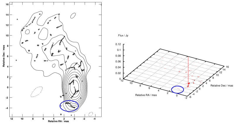
?figurename? 4.1: Plotting Clean components to reveal their relative strengths. Left panel: 5.0 GHz contour map of the polarization calibrator 1159+2914 observed in September 2002. Crosses indicate the locations of Clean components. Right Panel: The Clean components from the same image plotted to reveal their relative strengths. This representation reveals that almost the entire flux is concentrated in the central peak, and, e.g., that the group of components in the blue ellipses can be neglected in the $D$-term calibration. As a consequence, the calibration was done using a single component model.

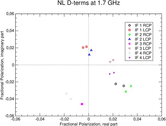
4.2.1 NL $D$-terms at 1.7 GHz on September 22, 2002.

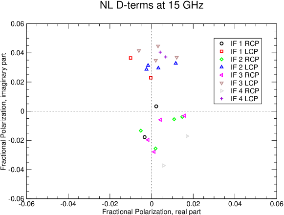
4.2.2 NL $D$-terms at 15.4 GHz on July 5, 2002.

?figurename? 4.2: North Liberty $D$-terms at 1.7 GHz and 15.4 GHz derived from the September 22, 2002 and July 5, 2002 observations, respectively. Each colour represents the measurements of a $D$-term in a specific IF, derived from observations of two calibrators. The scatter is representative of the polarization calibration of the array on these days (i.e., there are antennas with both smaller and larger scatter). The $D$-terms change systematically between the IFs at 1.7 GHz, whereas there is no such trend at 15.4 GHz. This reflects the different fractional bandwidths, 0.47 % at 1.7 GHz and 0.05 % at 15.4 GHz.

The quality of the calibration can be estimated by comparing the $D$-term solutions from the two polarization calibrators; two examples are shown in Fig. 4.2. The $D$-terms derived from the September 2002 observations of NGC 3079 (with the exception of the 2.3 GHz $D$-terms, see below) and from the July 2002 observations of Cygnus A were very good and consistent among the two calibrators. The $D$-terms derived from the July 2002 observations of NGC 4261, Hydra A and Centaurus A were a little less well constrained, but still of good quality. To obtain the most sensitive polarization images, however, images were made from this epoch without the stations at Mauna Kea, Hancock and Saint Croix, whose $D$-terms showed large scatter. These images did not differ significantly from those that were made from all data, and the polarization calibration was considered to be final. We have estimated the detection limit of polarized emission as follows: two polarization images of a calibrator were made from the same set of calibrated $(u,v)$ data and using the same imaging parameters (weighting, number of iterations of Clean, etc), but in one case using the $D$-terms derived from the calibrator itself and in the other case using the $D$-terms derived from the other calibrator. The polarized intensity images were divided by the associated total intensity images to obtain two images of fractional polarization of the calibrator. Finally, the fractional polarization images were differenced, and the average difference was measured over the source region. The average differences in fractional polarization were found to be 0.3 % for the observations of NGC 3079 at 1.7 GHz and 5.0 GHz; 0.5 % for NGC 1052; 1 % for NGC 4261, Hydra A and Centaurus A; and 0.3 % for Cygnus A.

A special problem occurred during the $D$-term calibration of the NGC 3079 2.3 GHz observations. The $D$-term amplitudes were unusually large, around 5 % in both RCP and LCP, and clustered around $-160^{\circ}$ (RCP) and $-100^{\circ}$ (LCP) degrees, whilst the 1.7 GHz and 5.0 GHz were of the order of 1 % to 2 %. Surprisingly, the $D$-terms were similar at all antennas, suggesting a connection to the antenna structure. A feature of the 2.3 GHz system at the VLBA is the presence of a dichroic beamsplitter in the optical path for simultaneous observations at 2.3 GHz and 8.4 GHz, the so-called geodetic S/X-band mode. The beamsplitter is a permanently installed piece of circuit board with an imprinted copper pattern that efficiently reflects emission at 8.4 GHz away from the feed onto a mirror over the 8.4 GHz feed horn.

Applying the $D$-terms to the calibrator data yielded fractional polarizations of 0.8 % and 1.7 %, respectively. Applying the $D$-terms to the NGC 3079 data, however, yielded a fractional polarization of about 5 %, whilst it was unpolarized at 1.7 GHz and 5.0 GHz. A fractional polarization of the same order as the $D$-terms is highly unlikely. The beamsplitter in the 2.3 GHz optical path might explain the unusual similarities of the $D$-terms and their particularly high amplitudes. But it does not explain why the systematic effect has not been calibrated on NGC 3079. We have explored numerous variations to the calibration strategy, e.g., changing the partitioning of the calibrator sources into sub-models, repeating the calibration without exporting the data to Difmap and different data weightings, but without success. We therefore do not present a 2.3 GHz polarization image of NGC 3079.

The final images are shown in Figs. 4.3 to 4.19. Figs. 4.9-4.19 have superimposed polarization ticks, except for the NGC 3079 2.3 GHz image in Fig. 4.10, and display the fractional polarization as colours. The lowest contours have been set to three times the image rms noise, and the polarization ticks have been cut off below five times the polarization image rms, except for the Cygnus A image, where the polarization has been cut off below seven times the polarization image rms to emphasise the detection.

4.3 The Images

			Beam parameters
Source	Epoch	Frequency	$b_{\rm maj}$	$b_{\rm min}$	P.A.	Peak	rms	Dyn.	P-Peak	P-rms	Dyn.
		GHz	mas	mas	degrees	${\rm mJy\,beam^{-1}}$		range	${\rm mJy\,beam^{-1}}$		range
(1)	(2)	(3)	(4)	(5)	(6)	(7)	(8)	(9)	(10)	(11)	(12)
NGC 3079	Nov 20, 1999	5.0	1.92	1.07	-30	20	0.08	270:1
		15.4	3.10	1.66	36	45	0.34	140:1
NGC 3079	Mar 6, 2000	5.0	1.20	0.85	-29	17.1	0.06	270:1
		15.4	2.01	1.33	-56	51	0.35	150:1
NGC 3079	Nov 30, 2000	5.0	1.40	0.87	-23	17.8	0.06	290:1
		15.4	2.25	1.69	-24	51	0.27	210:1
NGC 3079	Sep 22, 2002	1.7	5.12	3.49	-22	9.1	0.06	140:1	0.29a	0.04	7.3
		2.3	6.02	4.34	12	19.8	0.13	150:1
		5.0	3.86	3.11	-40	22	0.11	200:1	0.43a	0.05	8.6
NGC 1052	Dec 28, 2001	13.4	1.49	0.58	-4	344	0.36	960:1	1.36a	0.15	9.1
		15.4	1.33	0.50	-5	245	0.32	770:1	1.39a	0.16	8.7
NGC 4261	Jul 5, 2002		1.07	0.60	-6	129	0.18	720:1	0.83	0.09	9.2
Hydra A	Jul 5, 2002		1.58	0.56	3	144	0.29	500:1	1.81a	0.20	9.1
Centaurus A	Jul 5, 2002	13.4	2.09	0.47	0	1080	10.87	100:1	7.98	0.71	11.2
		15.4	2.15	0.42	1	907	7.46	120:1	9.91	1.05	9.4
Cygnus A	Jul 7, 2002	15.4	0.59	0.34	-21	316	0.23	1400:1	1.39	0.11	12.6

?tablename? 4.2: Image parameters. $a$: the peak in polarized intensity is outside the image shown.

4.3.1 NGC 3079

The first three epochs of NGC 3079 shown in Figs. 4.3-4.8 were observed using identical setups and have comparable quality. They show three components at 5.0 GHz and two components at 15.4 GHz. These epochs have about twice the resolution of the fourth epoch, because they included Effelsberg at 5.0 GHz and 15.4 GHz.

• 5.0 GHz  Our images display three compact components and an elongated feature between the southern and the western feature. Based on this morphology and adopting the notation from Irwin & Seaquist (1988), we identify the components as $A$ (south-east), $B$ (west) and $C$ (in between $A$ and $B$). The compact component north of $A$ was not detected by earlier 5 GHz observations, and we name it $E$. Component $A$ is the strongest component at 5.0 GHz, causing fringe-fitting to shift it to the image centre. It is compact and shows only a little extension to the north-west, in direction of $B$ and the jet-like feature $C$ on the $A$-$B$ axis. Component $B$ is resolved, which is clearly visible in the second and third epoch, where it is resolved into three sub-components. Component $E$ is also resolved, and its major axis has rotated from north-south in the first epoch (Fig. 4.3) to east-west in the third epoch (Fig. 4.7). The jet-like component $C$ is continuous in the first and second epoch and resolved into sub-components in the third epoch.

• 15.4 GHz  Our images show two compact components. Based on the separation and relative P.A. of the two matching that of $A$ and $B$ at 5.0 GHz, we identify the component towards the east with $A$ and the component towards the west with $B$. Our identification is further supported by 22 GHz observations by Trotter et al. (1998) who detected $A$ and $B$ with similar separation and relative P.A., and by 8.4 GHz observations by Kondratko (2003), who noticed that $E$ is fading towards higher frequencies and probably becoming invisible at 15 GHz and that $A$ and $B$ were still strong at this frequency. Thus, our identification appears to be correct, although we detect neither $E$ nor $C$ at 15.4 GHz. $A$ and $B$ are compact in all epochs, and component $B$ is the strongest at 15.4 GHz, so it is in the image centre. Fringe-fitting flags data that have too low SNR, and the remaining data of the first two epochs (Figs. 4.4 and 4.6) were distributed over a pronounced elliptical $(u,v)$ coverage, causing an almost $90^{\circ}$ change in position angle of the synthesized beam. This also caused the change in position angle of the major axes of $A$ and $B$. No detections were made on baselines to Effelsberg, Mauna Kea, Hancock and Y1 during the first epoch, to Effelsberg, Mauna Kea and St. Croix during the second epoch and to Brewster, Effelsberg, Hancock, Mauna Kea and St. Croix in the third epoch. These are predominantly long ($>100\,{\rm M\lambda}$) baselines, so that the resolution at 15.4 GHz during these epochs is lower than at 5.0 GHz.

  The flux densities of $A$ and $B$ changed on a significant level, especially between epoch two and three (Figs. 4.6 and 4.8), where $A$ brightened remarkably. The ratio of the peak flux densities, $S_{\nu,A}/S_{\nu,B}$, is $0.19\pm 0.01$ in epoch one, $0.11\pm 0.01$ in epoch two and $0.28\pm 0.02$ in epoch three. The changes have a significance of $9\,\sigma$ and $8\,\sigma$, respectively, and cannot be due to amplitude calibration errors because they scale the flux density of both components by the same factor, leaving the ratio constant.

In the fourth epoch of NGC 3079, Effelsberg did not observe at 2.3 GHz and 5.0 GHz, and so the beam size was significantly larger than in the first three epochs.

• 1.7 GHz (Fig. 4.9)  Two components are visible, a more compact one to the north-west and an extended one to the south-east. The south-eastern component, we named $F$, is the strongest at 1.7 GHz but is barely visible at 5.0 GHz. Due to their similar separation and relative position angle, $E$ and $F$ are easily misidentified with $A$ and $B$ (as unfortunately happened to Sawada-Satoh et al. 2000), but phase-referencing allowed us to identify the north-western component with component $E$ seen at 5.0 GHz during the same epoch. All components are unpolarized, and neither $A$, nor $B$ nor $C$ were detected at 1.7 GHz.

• 2.3 GHz (Fig. 4.10)  Three components are visible. Component $E$ is the strongest, while $F$ has become much fainter compared to the detection at 1.7 GHz. Component $A$, although weak, is reliably detected, whereas component $B$ is not seen.

• 5.0 GHz (Fig. 4.11)  The well-known triple structure appears to be almost unchanged since the previous epoch in 2000. Component $A$ is compact, component $B$ is slightly extended in the north-south direction, and $E$ is extended east-west. Due to the lower resolution, $C$ appears to be connected to $A$ and is not resolved into sub-components. $F$ is very weak at 5.0 GHz. All components are unpolarized.

Component $D$ seen by Trotter et al. (1998) was not detected in any of our observations.

The observations from 2002 and the 15.4 GHz observation from November 2000 were used to compose a four-colour image of NGC 3079, in which red corresponds to 1.7 GHz, yellow to 2.3 GHz as, green to 5.0 GHz and blue to 15.4 GHz (Fig. 4.12). We prefer this somewhat arbitrary transfer function of frequencies to colours because a linear transfer function would map the frequencies of 1.7 GHz to 5.0 GHz into those 35 % of the visible wavelengths (380 nm to 780 nm) that appear as red. This is due to the large gap between 5.0 GHz and 15.4 GHz. The colour representation that we chose emphasises the spectral differences of the components.

Additional Results from NGC 3079

The observations presented in this thesis allow a more detailed study of NGC 3079 than for the other five objects. To parameterize the observations, integrated flux densities and component positions have been measured (Table 4.3. The images in this chapter display the “best” images with full resolution obtained from each particular dataset. To minimise resolution effects and peak shifts due to changing imaging parameters, integrated flux densities and positions have been measured from uniformly weighted images tapered to a common resolution of $4\,{\rm mas}\times 3\,{\rm mas}$ (not shown).

The integrated flux densities have then been measured by summing over the pixels of the source region. This method is also sensitive to very weak and possibly extended emission which is below the lowest contour in the images shown. If a well-defined component was visible, positions have been measured by fitting a two-dimensional parabola to the brightest and the eight surrounding pixels from the images tapered to $4\,{\rm mas}\times 3\,{\rm mas}$ resolution. The fits also yielded peak flux densities. This procedure was found superior to fitting Gaussians because the sources were not always well described by a Gaussian.

In the cases of component $F$ at 5.0 GHz and component $B$ at 2.3 GHz, no component is visible in the contour plots (i.e., the peak flux density was below $3\,\sigma$), but significant flux density was measured over the regions where they are visible at other frequencies. In the case of $F$ at 5.0 GHz, the emission is weak and probably also resolved due to the lack of short $(u,v)$ spacings. We therefore give the flux densities in Table 4.3, but do not give coordinates, because our procedure to measure peak flux densities did not yield meaningful results in these cases. We estimate the flux density errors to be of the order of 5 %, in agreement with the VLBA’s observational status summary and with what is commonly adopted in the literature for VLBA observations. Exploring five images from a reasonable imaging parameter space revealed a position uncertainty of 0.15 mas ($1\,\sigma$).

The data presented in Table 4.3 can be used to derive spectral indices and component positions. Only the fourth epoch was phase-referenced and provides absolute coordinates. For the proper motion analysis, we therefore give the relative separations among the three components $A$, $B$ and $E$, because they are well-defined and visible during all epochs. Spectral indices and relative positions are given in Tables 4.4 and 4.5. Assuming a $1\,\sigma$ error of 5 % for the integrated flux densities yields spectral index errors of 0.09 for the 5.0 GHz/15.4 GHz and 1.7 GHz/5.0 GHz pairs, 0.33 for the 1.7 GHz/2.3 GHz pair and 0.13 for the 2.3 GHz/5.0 GHz pair. Each position has an error of 0.15 mas, so that separations have errors of $\sqrt{2}\times 0.15\,{\rm mas}=0.21\,{\rm mas}$.

		full resolution			tapered
Epoch	Freq.	$S$	$S_{\rm max}$	$x$	$S$	$S_{\rm max}$	$x$	RA	Dec
		Component $A$
Nov 20, 1999	5.0	27	21	0.78	28	25	0.89	-	-
	15.4	9.59	6.30	0.66	9.03	6.21	0.69	-	-
Mar 6, 2000	5.0	26	17	0.65	26	24	0.92	-	-
	15.4	14.8	6.81	0.46	6.75	7.02	1.04	-	-
Nov 30, 2000	5.0	23	17.8	0.77	24	23	0.96	-	-
	15.4	19.0	15.1	0.79	18.4	17.5	0.95	-	-
Sep 22, 2002	1.7	-	-		-	-	-	-	-
	2.3	1.88	1.24	0.66	2.45	1.13	0.46	57.80373	47.2436
	5.0	25	22	0.88	26	22	0.85	57.80368	47.2430
		Component $B$
Nov 20, 1999	5.0	14.9	6.92	0.46	16.9	13.9	0.82	-	-
	15.4	51	45	0.88	48	46	0.96	-	-
Mar 6, 2000	5.0	19.4	5.86	0.30	17.9	14.6	0.82	-	-
	15.4	59	51	0.86	59	54	0.92	-	-
Nov 30, 2000	5.0	19.2	8.05	0.42	18.7	14.6	0.78	-	-
	15.4	68	51	0.75	66	62	0.94	-	-
Sep 22, 2002	1.7	-	-		-	-	-	-	-
	2.3	-	-		0.64	-	-	-	-
	5.0	22	14.4	0.66	22	14.8	0.67	57.80112	47.2594
		Component $E$
Nov 20, 1999	5.0	4.14	1.61	0.39	4.12	3.45	0.84	-	-
	15.4	-	-		-	-	-	-	-
Mar 6, 2000	5.0	3.28	1.04	0.32	2.99	3.22	1.08	-	-
	15.4	-	-		-	-	-	-	-
Nov 30, 2000	5.0	7.18	1.42	0.20	5.14	3.96	0.77	-	-
	15.4	-	-		-	-	-	-	-
Sep 22, 2002	1.7	5.43	4.23	0.78	3.75	2.94	0.78	57.80429	47.2633
	2.3	21	19.8	0.94	18.0	19.8	1.10	57.80420	47.2605
	5.0	7.78	5.41	0.70	7.77	5.57	0.72	57.80413	47.2603
		Component $F$
Nov 20, 1999	5.0	-	-		4.12	-	-	-	-
	15.4	-	-		-	-	-	-	-
Mar 6, 2000	5.0	-	-		3.80	-	-	-	-
	15.4	-	-		-	-	-	-	-
Nov 30, 2000	5.0	-	-		2.88	-	-	-	-
	15.4	-	-		-	-	-	-	-
Sep 22, 2002	1.7	15.3	9.71	0.64	17.1	9.30	0.54	57.80632	47.2521
	2.3	7.18	2.11	0.29	9.31	2.18	0.23	57.80596	47.2530
	5.0	6.89	-		8.32	-	-	-	-

?tablename? 4.3: NGC 3079 component data. “Tapered” flux densities have been measured from images tapered to the same resolution and convolved with a beam of $4\,{\rm mas}\times 3\,{\rm mas}$. “Full resolution” flux densities have been measured from images using all available data. In September 2002, the tapered images differed only marginally from the full resolution images. Integrated flux densities, $S$, are given in mJy, peak flux densities, $S_{\rm max}$, are given in mJy beam^-1, the ratio $x=S_{\rm max}/S$ is dimensionless, coordinates are seconds of right ascension relative to 10:01:00 and arcseconds of declination relative to 55:40:00. Only the the last epoch used phase-referencing and hence provides coordinates measured with respect to the phase calibrator J0957+5522 at RA 09:57:38.1849709 and Dec +55:22:57.769241. When a flux density, but no position is given, the emission is very extended and possibly also faint, sometimes not being visible in the images. The relative separations of the components measured during all four epochs are listed in Table 4.5.

Epoch	SI	$A$	$B$	$E$	$F$
1999-11-20	$\alpha^{5.0}_{15.4}$	-0.99	0.92	$<-1.24$	-
2000-03-06	$\alpha^{5.0}_{15.4}$	-1.19	1.06	$<-0.93$	-
2000-11-30	$\alpha^{5.0}_{15.4}$	-0.25	1.13	$<-1.64$	-
2002-09-22	$\alpha^{1.7}_{2.3}$	$>8.52$	$>4.14$	5.11	$-1.64$
	$\alpha^{2.3}_{5.0}$	3.02	$4.52$	$-1.07$	$-0.28$
	$\alpha^{1.7}_{5.0}$	$>4.56$	$>4.41$	0.67	$-0.67$

?tablename? 4.4: Spectral indices of NGC 3079 components. Limits have been calculated using three times the image rms. Assuming a $1\,\sigma$ error of 5 % for the integrated flux densities yields spectral index errors of 0.09 for the 5.0 GHz/15.4 GHz and 1.7 GHz/5.0 GHz pairs, 0.33 for the 1.7 GHz/2.3 GHz pair and 0.13 for the 2.3 GHz/5.0 GHz pair. Although our observations were designed to avoid resolution effects, we cannot rule out that the spectral index of $F$ is affected by its extend and by some of the 2.3 GHz flux density missing due to the lack of short baselines.

Epoch	Freq.	$A-B$			$B-E$			$A-E$
		$\Delta{\rm RA}$	$\Delta{\rm Dec}$	$\Theta$	$\Delta{\rm RA}$	$\Delta{\rm Dec}$	$\Theta$	$\Delta{\rm RA}$	$\Delta{\rm Dec}$	$\Theta$
1999-11-20	5.0	21.1	15.5	26.2	26.2	1.5	26.3	5.1	17.0	17.7
	15.4	21.1	16.5	26.8	-	-	-	-	-	-
2000-03-06	5.0	21.3	15.6	26.4	26.1	1.4	26.2	4.8	17.0	17.7
	15.4	21.2	16.3	26.8	-	-	-	-	-	-
2000-11-30	5.0	21.3	15.8	26.5	25.9	1.2	25.9	4.6	17.0	17.6
	15.4	21.3	16.2	26.8	-	-	-	-	-	-
2002-09-22	1.7	-	-	-	-	-	-	-	-	-
	2.3	-	-	-	-	-	-	-	-	-
	5.0	21.7	16.4	27.2	25.5	0.9	25.5	3.8	17.3	17.7

?tablename? 4.5: Relative positions of NGC 3079 components. All separations are in mas and have errors of 0.21 mas

Epochs	Freq.	$A-B$		$B-E$		$A-E$
		$\Delta\Theta$	$v$	$\Delta\Theta$	$v$	$\Delta\Theta$	$v$
		mas	$c$	mas	$c$	mas	$c$
1999-11-20/	5.0	0.2	0.16	0.1	0.08	0.0	0.0
2000-03-06	15.4	0.0	0.0	-	-	-	-
2000-03-06/	5.0	0.1	0.03	0.2	0.07	0.1	0.03
2000-11-30	15.4	0.0	0.0	-	-	-	-
2000-11-30/	5.0	0.7	0.09	0.4	0.05	0.1	0.01
2002-09-22

?tablename? 4.6: Proper motions derived from separations in Table 4.5. $\Delta\Theta$ has errors of 0.21 mas, and hence $v$ has errors of $0.17\,c$, $0.07\,c$ and $0.03\,c$ in the first, second and third row, respectively.

4.3.2 NGC 1052

The 13.4 GHz and 15.4 GHz images of NGC 1052 are shown in Figs. 4.13 and 4.14. The excellent agreement between these two images confirms that the data calibration and the imaging process were correct. Furthermore, our 15.4 GHz image nicely fits into the time series of images shown by Vermeulen et al. (2003). Compared to their last epoch observed in 2001.21 (ours being observed at 2001.99), some significant evolution is visible in the two inner and most compact components, whereas the outer extended components appear to be unchanged.

• 13.4 GHz (Fig. 4.13)  The image shows the well-known pronounced double-sided jet structure, dominated by a central component with an extension to the west. The eastern jet is stronger than the western jet and widens at 5 mas distance from the strongest feature in the image centre. It then gently narrows to 2 mas width before it fades in an extended, low surface-brightness feature. The western jet displays a bright, compact component with a clear extension in the direction of the jet axis and is connected by a very weak bridge of emission to the main component. There is a sharp transition to a weak, continuous feature that bridges 3 mas to the next, extended jet feature. Further down the western jet is a weak, isolated component. NGC 1052 is entirely unpolarized at 13.4 GHz.

• 15.4 GHz (Fig. 4.14)  This image differs only little from the 13.4 GHz image. Due to the slightly higher resolution, the main component is more clearly resolved into two components, and, probably due to a negative spectral index, the connection to the eastern jet has become weaker. The weak object at the end of the eastern jet has dimmed to the one-contour level and is disconnected from the jet. The connection between the two brightest components was not detected, now leaving a gap between them. Compared to the 13.4 GHz image, the changes in the western jet are marginal. NGC 1052 is entirely unpolarized at 15.4 GHz.

4.3.3 NGC 4261

The 15.4 GHz image in Fig. 4.15 displays a double-sided, continuous structure. The central feature gently fades into the western jet that extends out to 9 mas from the core. Compared to this transition, there is a rather sharp drop-off between the central peak and the eastern jet due to the circumnuclear disc. The polarization ticks 2 mas south-west of the core have a maximum of $0.68\,{\rm mJy\,beam^{-1}}$ at a position where the total intensity is $14.4\,{\rm mJy\,beam^{-1}}$ (4.7 % fractional polarization). The polarization was found to change considerably when the imaging parameters (weighting, tapering) were changed. They are probably due to residual deconvolution errors. We therefore conclude that NGC 4261 is entirely unpolarized.

NGC 4261 has previously not been observed at 15.4 GHz, and we therefore compare our image to the 8.4 GHz and 22.2 GHz images by Jones & Wehrle (1997) and Jones et al. (2000). NGC 4261 is undergoing considerable spectral evolution between these two frequencies, and our image nicely fits inbetween. At 8.4 GHz, the absorbed gap in front of the counter-jet is clearly visible. At 15.4 GHz, the absorber is manifest by somewhat denser isophotes $<1\,{\rm mas}$ east of the core, and at 22.2 GHz, there is almost no indication of the absorber. The lengths of the jet and counter-jet are shorter at 15.4 GHz than at 8.4 GHz, and shorter at 22.2 GHz than at 15.4 GHz. This is due to the negative spectral index, the longer integration time used at 8.4 GHz and the higher sensitivity at this frequency.

4.3.4 Hydra A

The 15.4 GHz image in Fig. 4.16 shows a relatively small, double-sided core-jet structure, the transitions from the core into the jets being equally smooth on both sides. Aside from the jets, a weak component was detected 3 mas south-west of the core which is connected to the jets via a weak bridge of emission. Hydra A is entirely unpolarized.

We see no significant structural difference between our image and the 15.4 GHz image shown by Taylor (1996). The peak flux density in our image, $(144\pm 7)\,{\rm mJy\,beam^{-1}}$, is higher than the integrated flux density reported by Taylor (1996), $(127\pm 6)\,{\rm mJy}$, but almost in agreement within the errors.

4.3.5 Centaurus A

The 13.4 GHz and 15.4 GHz images are shown in Figs. 4.17 and 4.18. The iterative self-calibration and cleaning was found to give multiple solutions due to the poor $(u,v$) coverage at the source declination of $-43^{\circ}$. The similarity of the final images, however, indicates that the calibration of both frequencies has converged on the most likely source structure.

• 13.4 GHz  The image in Fig. 4.17 shows a core and a single-sided jet structure extending over almost 10 mas to the north-east. The flux density drops off to 25 % of the peak flux density within the first 1.5 mas, reaches a plateau and fades at 8 mas core distance. Large noise patches surrounding the source and a high image rms indicate significant sidelobes. Centaurus A has a formally significant degree of polarization of 4.9 %, but there are also formally significant regions of polarization outside the source area which obviously are due to deconvolution errors. These lie outside the region shown in Fig. 4.17, but similar effects can be seen in the 15.4 GHz image in Fig. 4.18. We therefore consider Centaurus A to be unpolarized at 13.4 GHz.

• 15.4 GHz  The image in Fig. 4.18 is similar to the 13.4 GHz image, the only difference being a barely visible bend in the jet base close to the core. A detection of this bend has been claimed by Fujisawa et al. (2000) from VLBI observations at $4.8\,{\rm GHz}$, but their $(u,v)$ coverage was extremely sparse. Tingay et al. (2001) have monitored the source during eight epochs at frequencies of up to 22 GHz and did not detect such a bend in any of their epochs, and we interpret the bend claimed by Fujisawa et al. (2000) as an imaging artefact. We consider the polarization seen in this image as being due to deconvolution errors, like in the 13.4 GHz image.

Our images have considerably higher resolution ($2\,{\rm mas}\times 0.5\,{\rm mas}$) than the 8.4 GHz images ($13\,{\rm mas}\times 3\,{\rm mas}$) and the 22.2 GHz images ($5\,{\rm mas}\times 1\,{\rm mas}$) presented by Tingay et al. (2001). Hence, most of the jet structure and also the weak, extended counter-jet feature seen by these authors is resolved out in our images.

4.3.6 Cygnus A

The 15.4 GHz image in Fig. 4.19 shows a continuous double-sided jet structure spanning more than 12 mas. The core appears to be elongated and slightly bean-shaped. The eastern jet comprises a compact component of 1 mas extend and a weak, extended component 2 mas to 4 mas east of the core. The western jet has a brightness temperature similar to that of the compact component in the eastern jet, but extends further out. At a position 3.5 mas west of the core, the flux density sharply drops to less than 1 % of the peak flux density, and a diffuse, irregular structure of almost 5 mas length marks the continuation of the jet. Cygnus A is the only source presented here that shows significant, believable polarization. The central region shows $1.4\,{\rm mJy\,beam^{-1}}$ of polarized emission on top of a Stokes I peak of $316\,{\rm mJy\,beam^{-1}}$, i.e., the region is 0.44 % polarized. The $D$-term calibration in this data set was very good, and the image has the highest dynamic range of all observations presented here (1400:1). Furthermore, the data calibration was repeated independently by a colleague who found very similar results (U. Bach, priv. comm.). We therefore conclude that Cygnus A is polarized.

Our image displays basically the same structure as has been found by Bach et al. (2003), although a comparison is difficult due to the higher resolution in our image that was caused by the participation of Effelsberg. The faint and extended jet and counter-jet structures in our image are therefore resolved and weaker than in the image by Bach et al. (2003).

?figurename? 4.3: NGC 3079 5.0 GHz VLBA+EB+Y1 image from November 20, 1999. Peak is $20\,{\rm mJy\,beam^{-1}}$, contours are at $\rm{0.23\,mJy\,beam^{-1}}\times 2^{N}$, natural weighting, beam is $1.92\,{\rm mas}\times 1.07\,{\rm mas}$ in P.A. $-30^{\circ}$.

?figurename? 4.4: NGC 3079 15.0 GHz VLBA+EB+Y1 image from November 20, 1999. Peak is $45\,{\rm mJy\,beam^{-1}}$, contours are at $\rm{1.02\,mJy\,beam^{-1}}\times 2^{N}$, natural weighting, beam is $3.10\,{\rm mas}\times 1.66\,{\rm mas}$ in P.A. $36^{\circ}$.

?figurename? 4.5: NGC 3079 5.0 GHz VLBA+EB+Y1 image from March 6, 2000. Peak is $17.1\,{\rm mJy\,beam^{-1}}$, contours are at $\rm{0.19\,mJy\,beam^{-1}}\times 2^{N}$, natural weighting, beam is $1.20\,{\rm mas}\times 0.85\,{\rm mas}$ in P.A. $-29^{\circ}$.

?figurename? 4.6: NGC 3079 15.0 GHz VLBA+EB+Y1 image from March 6, 2000. Peak is $51\,{\rm mJy\,beam^{-1}}$, contours are at $\rm{1.05\,mJy\,beam^{-1}}\times 2^{N}$, natural weighting, beam is $2.01\,{\rm mas}\times 1.33\,{\rm mas}$ in P.A. $-56^{\circ}$.

?figurename? 4.7: NGC 3079 5.0 GHz VLBA+EB+Y1 image from November 30, 2000. Peak is $17.8\,{\rm mJy\,beam^{-1}}$, contours are at $\rm{0.18\,mJy\,beam^{-1}}\times 2^{N}$, natural weighting, beam is $1.40\,{\rm mas}\times 0.87\,{\rm mas}$ in P.A. $-23^{\circ}$.

?figurename? 4.8: NGC 3079 15.0 GHz VLBA+EB+Y1 image from November 30, 2000. Peak is $51\,{\rm mJy\,beam^{-1}}$, contours are at $\rm{0.82\,mJy\,beam^{-1}}\times 2^{N}$, natural weighting, beam is $2.25\,{\rm mas}\times 1.69\,{\rm mas}$ in P.A. $-24^{\circ}$.

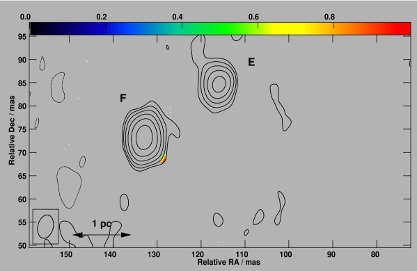
?figurename? 4.9: NGC 3079 1.7 GHz VLBA+EB image from September 2002. Peak $9.70\,{\rm mJy\,beam^{-1}}$, contours $0.19\,\rm{mJy\,beam^{-1}}\times 2^{N}$, nat. weighting, beam $5.12\,{\rm mas}\times 3.49\,{\rm mas}$ in P.A. $-22^{\circ}$, pol. ticks $1\,{\rm mJy\,beam^{-1}\,mas^{-1}}$ where $>5\,\sigma=0.22\,{\rm mJy\,beam^{-1}}$. Axes relative to RA 10 01 57.7906 Dec 55 40 47.1788 (J2000), colours show fractional polarization.

?figurename? 4.10: NGC 3079 2.3 GHz VLBA image from September 2002. Peak is $19.8\,{\rm mJy\,beam^{-1}}$, contours are at $0.39\,\rm{mJy\,beam^{-1}}\times 2^{N}$, natural weighting, beam is $6.02\,{\rm mas}\times 4.34\,{\rm mas}$ in P.A. $12^{\circ}$. Axes relative to RA 10 01 57.7906 Dec 55 40 47.1788 (J2000).

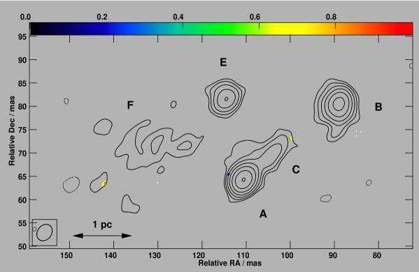
?figurename? 4.11: NGC 3079 5.0 GHz VLBA image from September 2002. Peak $21.64\,{\rm mJy\,beam^{-1}}$, contours $\rm{0.33\,mJy\,beam^{-1}}\times 2^{N}$, nat. weighting, beam $3.86\,{\rm mas}\times 3.11\,{\rm mas}$ in P.A. $-40^{\circ}$, pol. ticks $1\,{\rm mJy\,beam^{-1}\,mas^{-1}}$ where $>5\,\sigma=0.27\,{\rm mJy\,beam^{-1}}$. Axes relative to RA 10 01 57.7906 Dec 55 40 47.1788 (J2000), colours show fractional polarization.

?figurename? 4.12: Four-colour image of NGC 3079, composed of the observations from 2002 and the 15.4 GHz observations from November 2000. 1.7 GHz is represented as red, 2.3 GHz as yellow, 5.0 GHz as green and 15.4 GHz as blue.

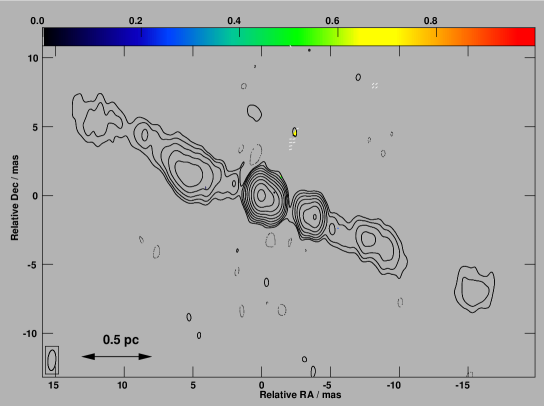
?figurename? 4.13: NGC 1052 13.4 GHz VLBA image. Peak is $344\,{\rm mJy\,beam^{-1}}$, contours are at $\rm{1.08\,mJy\,beam^{-1}}\times 2^{N}$, uniform weighting, beam is $1.49\,{\rm mas}\times 0.58\,{\rm mas}$ in P.A. $-4^{\circ}$, pol. ticks are $5\,{\rm mJy\,beam^{-1}\,mas^{-1}}$ where $>5\,\sigma=0.74\,{\rm mJy\,beam^{-1}}$, colours show fractional polarization.

?figurename? 4.14: NGC 1052 15.4 GHz VLBA image. Peak is $245\,{\rm mJy\,beam^{-1}}$, contours are at $\rm{0.94\leavevmode\nobreak\ mJy\,beam^{-1}}\times 2^{N}$, uniform weighting, beam is $1.33\,{\rm mas}\times 0.50\,{\rm mas}$ in P.A. $-5^{\circ}$, pol. ticks are $5\leavevmode\nobreak\ {\rm mJy\,beam^{-1}\,mas^{-1}}$ where $>5\,\sigma=0.80\,{\rm mJy\,beam^{-1}}$, colours show fractional polarization.

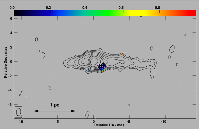
?figurename? 4.15: NGC 4261 15.4 GHz VLBA image. Peak is $129\,{\rm mJy\,beam^{-1}}$, contours are at $\rm{0.54\,mJy\,beam^{-1}}\times 2^{N}$, uniform weighting, beam is $1.07\,{\rm mas}\times 0.60\,{\rm mas}$ in P.A. $-6^{\circ}$, polarization ticks are $5\,{\rm mJy\,beam^{-1}\,mas^{-1}}$ where $>5\,\sigma=0.45\,{\rm mJy\,beam^{-1}}$, colours show fractional polarization.

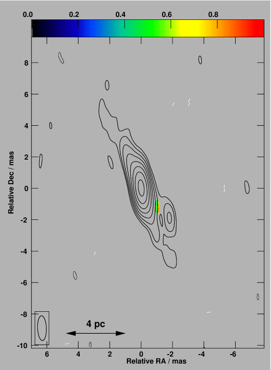
?figurename? 4.16: Hydra A 15.4 GHz VLBA image. Peak is $144\,{\rm mJy\,beam^{-1}}$, contours are at $\rm{0.87\,mJy\,beam^{-1}}\times 2^{N}$, uniform weighting, beam is $1.58\,{\rm mas}\times 0.56\,{\rm mas}$ in P.A. $3^{\circ}$. The length of the polarization ticks is $5\,{\rm mJy\,beam^{-1}\,mas^{-1}}$ and start at the polarization $5\,\sigma$ level of $1.00\,{\rm mJy\,beam^{-1}}$. Colours show fractional polarization.

?figurename? 4.17: Centaurus A 13.4 GHz VLBA image. Peak is $1.08\,{\rm Jy\,beam^{-1}}$, contours are at $\rm{32.61\,mJy\,beam^{-1}}\times 2^{N}$, uniform weighting, beam is $2.09\,{\rm mas}\times 0.47\,{\rm mas}$ in P.A. $0^{\circ}$, polarization ticks are $20\,{\rm mJy\,beam^{-1}\,mas^{-1}}$ where $>5\,\sigma=3.55\,{\rm mJy\,beam^{-1}}$, colours show fractional polarization.

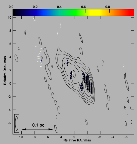
?figurename? 4.18: Centaurus A 15.4 GHz VLBA image. Peak is $907\,{\rm mJy\,beam^{-1}}$, contours are at $\rm{22.38\,mJy\,beam^{-1}}\times 2^{N}$, uniform weighting, beam is $2.15\,{\rm mas}\times 0.42\,{\rm mas}$ in P.A. $1^{\circ}$, polarization ticks are $20\,{\rm mJy\,beam^{-1}\,mas^{-1}}$ where $>5\,\sigma=5.25\,{\rm mJy\,beam^{-1}}$, colours show fractional polarization.

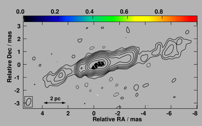
?figurename? 4.19: Cygnus A 15.4 GHz VLBA+EB+Y1 image. Peak is $316\,{\rm mJy\,beam^{-1}}$, contours are at $\rm{0.69\,mJy\,beam^{-1}}\times 2^{N}$, uniform weighting, beam is $0.59\,{\rm mas}\times 0.34\,{\rm mas}$ in P.A. $-21^{\circ}$, polarization ticks are $5\,{\rm mJy\,beam^{-1}\,mas^{-1}}$ where $>7\,\sigma=0.77\,{\rm mJy\,beam^{-1}}$, colours show fractional polarization.

?chaptername? 5 Discussion

The discussion of the observational results presented in the previous chapters is divided into two sections: one treating the polarimetry results and one treating the multi-epoch observations of NGC 3079, considering spectral indices, proper motions and general properties of nuclear radio components in Seyfert galaxies.

5.1 Polarimetry Results

5.1.1 Introduction

The jet in M87 was the first extragalactic jet in which polarized emission was found (Baade 1956), and was immediately identified as synchrotron emission. With synchrotron emission being established as the process by which AGN jets radiate in the radio regime, polarization measurements allowed investigations of magnetic field orientations and strengths, shock properties, and optical depths.

These investigations are based on the degree, orientation, location in the source and temporal evolution of polarized emission. A lack of polarized emission, however, is a fundamental observational difference between the sources observed for this thesis and most other AGN, and it indicates a process which is not commonly found. It would be an unnecessary complication to postulate a different intrinsic emission mechanism in polarized and unpolarized sources, given their similarities in so many other respects. We therefore believe that the emission process in the source is also synchrotron emission and therefore is intrinsically significantly polarized, and that the observed lack of polarized emission therefore is due to a depolarization mechanism or a blending effect. The mechanism(s) reprocess(es) the radiation either inside or outside the emitting regions, and we refer to them as “intrinsic” and “extrinsic” depolarization mechanisms, respectively. Because blending effects would also occur inside the sources, they are treated as an intrinsic depolarization mechanism.

5.1.2 Significance of Lack of Polarization

We first demonstrate the significance of our findings (significant polarized emission in only one out of six sources) by comparing our results to the samples by Kellermann et al. (1998) and Zensus et al. (2002). They have observed 171 compact sources at 15 GHz to investigate their jet structure and kinematics, and to derive statistical properties. The continuation of the project, known as the MOJAVE prgramme, has also polarimetric information on a statistically complete subsample (Lister 2003). This sample comprises all sources with declination $\delta>-20^{\circ}$, galactic latitude $|b|>2.5^{\circ}$ and total 15.4 GHz VLBA flux density of more than 1.5 Jy. The sources are core-dominated, beamed quasars because one of its goals was to test Monte-Carlo simulations of beaming in a flux-limited sample of jets. Preliminary results are available on the MOJAVE prgramme homepage. As of October 2003, 129 sources with polarization measurements were available (Lister, priv. comm.), with a detection limit of 0.3 % of fractional polarization. Given this limit, the sample has 10 unpolarized sources. In our sample, not considering Centaurus A due to the low image fidelity and NGC 3079 because it is clearly not a radio galaxy, three out of four sources are unpolarized. In a difference-of-two-proportions test with Yates correction for continuity, we find a probability of 0.03 % that the two samples have been drawn from the same parent distribution. If we require a detection limit of more than 0.6 % for the MOJAVE sample sources, equal to the averaged detection limit of our three 15 GHz observing runs in December 2001 and July 2002, 19 of the 129 sources in the MOJAVE sample are unpolarized. This subsample has a probability of 1.2 % of being drawn from the same parent distribution as our sources, and so the polarization properties of the two samples are significantly different.

Furthermore, the fraction of double-sided jets (sources with structure on more than one side of the brightest component) in our sample is four out of six. If we exclude NGC 3079 because it is not a radio galaxy, then the fraction is four out of five, and if Centaurus A is treated as a double-sided source, because a counter-jet is not prominent but some evidence has been found (Tingay et al. 2001), then the fraction is five out of five. In the MOJAVE sample, the number of double-sided sources is six out of 129. A difference-of-two-proportions test yields a probability of less than 0.01 % that the two samples have been drawn from the same parent distribution (the probability remains less than 0.01 % when Centaurus A is treated as a single-sided source).

Our sample selection criteria (free-free absorbers in front of a jet, sources bright enough for VLBI polarimetry at 15.4 GHz and closer than 200 Mpc), therefore selected sources with significantly different polarization characteristics compared to those satisfying the MOJAVE selection criteria (basically, sources brighter than 1.5 Jy at 15.4 GHz). However, the statements about the fraction of polarized sources and the single- and double-sidedness are not strong because our sample is small. Furthermore, the MOJAVE programme is flux-density limited at 15.4 GHz and so is biased towards highly beamed quasars.

5.1.3 Intrinsic Causes

Tangled Internal Magnetic Fields

If the emitting regions are optically thin, the radiation that one receives is the superposition of radiation from along the line of sight through the source. In this case, for a homogeneous magnetic field and a population of relativistic electrons with a power-law distribution of the form $N(E)\,dE=N_{0}\,E_{0}^{-p}\,dE$, the theoretical maximum of polarization is

$$m(p)=100\times\frac{3\,p+3}{3\,p+7}$$ (5.1)

(Le Roux 1961), where $m$ is the percentage of polarization. For $p=2$, $m(p)=70\,\%$, and these high degrees of polarization are in fact found in radio lobes (e.g., in Cygnus A, Carilli et al. 1989) and also in BL Lac objects (e.g., Gabuzda et al. 1994). In these cases, the magnetic fields must be very homogeneous on angular scales similar to or larger than the resolution of the instrument. In general, magnetic fields are not homogeneous, but are composed of a uniform component, $B_{0}$, and a random component, $B_{\rm r}$, which varies on a typical length scale, thus making “cells”, in which the magnetic field is homogeneous. Provided that $B_{\rm r}$ varies on scales much less than the source diameter, the intrinsic degree of polarization in each cell, $m_{\rm i}(p)$, is averaged over the source to the observed degree of polarization, $m_{\rm o}(p)$, given by

$$\begin{split}m_{\rm o}(p)&=m_{\rm i}(p)\times\frac{B^{2}_{0}}{B^{2}_{0}+B^{2}_{\rm r}}\\ &\approx\frac{\rm Energy\leavevmode\nobreak\ in\leavevmode\nobreak\ uniform\leavevmode\nobreak\ field}{\rm Energy\leavevmode\nobreak\ in\leavevmode\nobreak\ total\leavevmode\nobreak\ field}\\ \end{split}$$ (5.2)

(Burn 1966). For $p=2$, the fractional polarization in each cell is 70 %. To depolarize this below our detection threshold of 0.3 %, the magnetic field energy would need to be dominated by the random component by a factor of more than 200. The jets would have to be turbulent, and very little ordering of the magnetic fields by the overall outward motion of the jet flow would be permitted.

The fractional polarization decreases as $i^{-1/2}$, where $i$ is the number of independent magnetic cells across the emitting region (Jones & Odell 1977). To depolarize an intrinsic fractional polarization of 70 % to 0.3 % requires 54000 cells, and to depolarize an intrinsic fractional polarization of 10 % still requires 1100 cells. Thus, the jets would need to be interspersed throughout with randomly oriented magnetic fields, a situation which does not agree with two observational facts. First, AGN jets are shaped by magnetic fields from sub-pc to kpc scales, requiring at least some ordering of the fields in all parts of the jets. Second, jets evolve along their axes, which has been observed in many radio jets on parsec scales. Shocks in jets compress the magnetic fields and so leave behind regions of ordered magnetic fields (Laing 1980). Evolving jets have been observed in NGC 1052 (Vermeulen et al. 2003) and Cygnus A (Krichbaum et al. 1998), and it is therefore unlikely that these jets are dominated by random magnetic fields. Furthermore, turbulent magnetic fields require a source of energy to sustain the disorder because ordered fields have lower energy.

In the case of an optically thick source, the maximum intrinsic degree of polarization is 10 % to 12 % (Jones & Odell 1977), and one receives emission only from the surface. The same considerations as for the optically thin case apply, and to depolarize the radiation below the detection threshold requires more than 1100 cells across the observing beam, so that in this scenario, the magnetic fields inside the jets must be ordered to confine the jet, but must be turbulent in the radiating surface. The idea of such an outer boundary layer (also called shear layer) which is physically different from the jet interior has been raised for the first time by Owen et al. (1989) to explain their VLA observations of the kpc-scale jet of M 87. In the case of M 87, however, the boundary layer is optically thin, as indicated by up to 50 % of polarization (Perlman et al. 1999), and the magnetic field in the boundary layer is highly ordered, indicated by similar P.A. of the polarized emission over regions $>100\,{\rm pc}$ in size. On smaller spatial scales, evidence for boundary layers has been found in some BL Lac objects and FR I radio galaxies by, e.g., Gabuzda (2002) and Attridge et al. (1999). FR I radio galaxies and BL Lacs are thought to be similar objects, the difference being due to different inclination angles. Chiaberge et al. (2000) find that FR I radio galaxies are more luminous by factors of 10 to $10^{4}$ than predicted from spectral energy distributions of BL Lacs seen edge-on. They explain the discrepancy with a stratified jet structure, in which a highly relativistic spine is surrounded by slower (but still relativistic) layers. When viewed from smaller angles, emission from the beamed spine dominates the jet emission, and the jet morphology is that of a BL Lac. When viewed from larger angles, the beaming cone points away from earth, but emission from the unbeamed boundary layer remains, preventing the full 10 to $10^{4}$-fold decrease of luminosity, and the morphology is that of an FR I. Thus, there is theoretical and observational evidence for a region around radio jets that has different physical parameters than the jet inside.

However, there are considerable objections to the depolarization being due to jet boundary layers in the sources presented here. First, even though the physical properties of jet boundary layers are very much different from the embedded spine, that does not necessarily mean that the magnetic fields are turbulent. Observations of the distribution of polarized emission have yielded evidence for the existence of boundary layers, not against it (like the abovementioned observations by Perlman et al. 1999 and Attridge et al. 1999), and so the boundary layers must be ordered. Second, numeric models of jets by Aloy et al. (2000) show that the boundary layer magnetic field is well aligned with the jet direction, and third, Laing (1980) showed that compression of a volume with randomly oriented magnetic fields onto a plane almost always causes the radiation to be polarized by more than 10 %. Thus, only if the initial boundary-layer random field is uncompressed and the jet does not evolve and stretch the boundary layer magnetic fields, is there the possibility that the radiation from the boundary layer is unpolarized. Given the works mentioned above, we deem this situation very unlikely.

Internal Faraday Rotation

In the case of internal Faraday rotation, polarized emission from various depths along the line of sight through the source is Faraday-rotated by the source itself, the degree of rotation depending on the depth of the emitting region. Internal Faraday rotation is only significant at the transition from frequencies where the source is optically thick to where it becomes optically thin, because self-absorption goes as $\sim\nu^{-3}$, whereas Faraday rotation goes as $\nu^{-2}$, shallower than the self-absorption. Towards low frequencies, the $\tau=1$ surface (the depth in the source from which most emission is received) approaches the surface of the source, and only few material is left that participates in Faraday rotation. Towards high frequencies, the source becomes transparent, and all material contributes to the Faraday rotation, but the rotation measure quickly drops as $\nu^{-2}$ and the effect is small. Furthermore, internal Faraday rotation requires a significant fraction of “cold” electrons in the jet with low Lorentz factors ($\gamma_{\rm min}\approx 1$ to $10$), because the relativistic mass growth of the electrons at higher Lorentz factors reduces their response to the electric fields. As electrons in jets of radio galaxies are expected to be highly relativistic ($\gamma_{\rm min}\approx 100$), we do not consider this explanation further. However, there is the possibility that the situation in NGC 3079 is different. Modelling the NLR line emission to be powered by energy and momentum transfer from radio jets, Bicknell et al. (1998) find that electrons in Seyfert radio components may be only mildly relativistic.

Given the careful tuning of conditions that is required to explain the lack of polarized emission with intrinsic causes, and given how unlikely they are to be fulfilled, we prefer to reject those explanations, and the depolarization must have a different origin.

Both intrinsic and extrinsic depolarization mechanisms impose an upper limit on the typical length scale on which the magnetic field changes direction. Assuming that this scale is similar for all sources, the best limit is given by NGC 1052 at a distance of 19.4 Mpc, since it is the closest of the double-sided jet sources in which a solid non-detection was made. In NGC 1052, our highest resolution image at 15.4 GHz resolved 0.5 mas, corresponding to 0.047 pc in the source. Within a volume of 0.047 pc on a side, $i=54000$ independent cells are required to depolarize an intrinsic degree of 70 % polarization to the observed upper limit of 0.3 %. Thus, the typical length scale of a cell is $<1/\sqrt[3]{54000}$ of the observing beam, or 0.0012 pc. In the case of the source being optically thick, the typical cell size must still be $<1/10$ of the beam, or 0.0047 pc.

5.1.4 External Causes

Bandwidth Depolarization

At each wavelength, the electric vector position angle of the waves after passing through the medium is different, and integrating over the observing bandwidth yields an apparent net polarization that is lower than the initial state. The depolarization across the observing bandwidth can be calculated as follows. Consider an ensemble of waves with wavelengths $\lambda$ in the observed bandwidth $\Delta\lambda$, so that $\lambda_{0}<\lambda<\lambda_{0}+\Delta\lambda$. Let us assume that all waves have the same electric vector position angle. If the waves pass through a magnetized plasma, the electric vectors $\vec{E}(\lambda)$ are rotated by Faraday rotation.

Assuming that a homogeneously magnetized slab of plasma has a rotation measure $RM$, the change of EVPA with wavelength is given by

$$\begin{split}\theta(\lambda_{0})&=RM\times\lambda_{0}^{2}+\theta_{0}\\ \theta(\lambda_{1})&=RM\times\lambda_{1}^{2}+\theta_{0}\\ \Rightarrow\Delta\theta(\lambda_{1},\lambda_{0})&=RM(\lambda_{1}^{2}-\lambda_{0}^{2}),\\ \end{split}$$ (5.3)

where $\theta_{0}$ is the EVPA of the waves before passing through the medium and $\theta(\lambda)$ is the wavelength-dependent EVPA after passing through the medium. With respect to the reference wavelength $\lambda_{0}$, the electric vectors $\vec{E}(\lambda)$ are rotated by $\Delta\theta(\lambda_{1},\lambda_{0})$:

$$\begin{split}\vec{E}(\lambda)&=\vec{E}(\lambda_{0})e^{i\Delta\theta(\lambda,\lambda_{0})}\\ &=\vec{E}(\lambda_{0})e^{iRM(\lambda^{2}-\lambda_{0}^{2})}.\\ \end{split}$$ (5.4)

Integrating all vectors in the observing band yields

$$\begin{split}<\vec{E}>(\lambda_{1},\lambda_{0})&=\frac{1}{\lambda_{1}-\lambda_{0}}\int_{\lambda_{1}}^{\lambda_{0}}\vec{E}(\lambda)\,d\lambda\\ &=\frac{1}{\lambda_{1}-\lambda_{0}}\int_{\lambda_{1}}^{\lambda_{0}}\vec{E}(\lambda_{0})e^{iRM(\lambda^{2}-\lambda_{0}^{2})}\,d\lambda\\ &=\frac{\vec{E}(\lambda_{0})e^{-iRM\lambda_{0}^{2}}}{\lambda_{1}-\lambda_{0}}\int_{\lambda_{1}}^{\lambda_{0}}e^{iRM(\lambda^{2})}\,d\lambda\\ \end{split}$$ (5.5)

This integral can be solved numerically (Fig. 5.1), and one finds that for the radiation to be depolarized to $50\,\%$ of initial value requires $RM=2.2\times\,10^{6}$ in a 32 MHz wide band at 15.0 GHz. The largest values of RM that have been measured in quasar cores are a few thousands (e.g., Zavala & Taylor 2003). Assuming a rotation measure of $RM=10^{4}\,{\rm rad\,m^{-2}}$ causes $0.00012\,\%$ depolarization. Bandwidth depolarization is unlikely to be important because unprecedently high and uniform (to rotate the electric vector position angle in one direction only) rotation measures would be needed to depolarize the sources, requiring very uniform conditions in the Faraday screen.

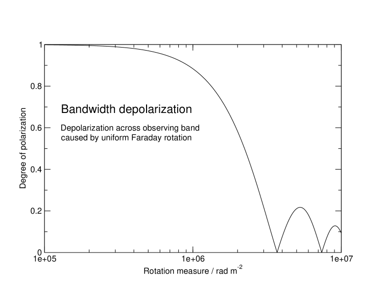
?figurename? 5.1: Bandwidth depolarization in the 15 GHz band.

Beam Depolarization

If the rotation measure in a foreground Faraday screen changes on angular scales much smaller than the observing beam, regions with similar degrees of polarization but opposite signs average out and the observed degree of polarization is decreased. Thus, spatially highly variable $RM$s can in principle depolarize the source. Estimates of $RM$ and the length scale on which the magnetic field needs to be tangled or the electron density changes follow similar approaches as in the previous sections. The electric vectors must be rotated by $180^{\circ}$ on average to remove any residual polarized emission, requiring the rms of the variations in the Faraday screen, $\sigma_{RM}$, to be

$$\begin{split}\theta(\lambda)&=\lambda^{2}\times RM\\ \Rightarrow RM&=\theta(\lambda)/\lambda^{2}\\ \Rightarrow\sigma_{RM}&=\frac{\pi\,{\rm rad}}{(c/15.4\,{\rm GHz})^{2}}=8290\,{\rm rad\,m^{-2}}\end{split}$$ (5.6)

or larger at 15.4 GHz. If the $RM$ changes are caused only by density fluctuations in the medium ($B_{\parallel}$ and $L$ constant), then the rms of the fluctuations is of the order of $10^{4}\,{\rm cm^{-3}}$. For NGC 3079, the constraints on the Faraday rotation are weaker because the highest frequency at which no polarized emission has been observed is 5.0 GHz, and so the rms of $RM$ must be $872\,{\rm rad\,m^{-2}}$ or more. The estimate of the rotation measure cell size was calculated in §5.1.3, yielding upper limits of 0.0012 pc to 0.0047 pc for NGC 1052, the closest double-sided source.

Free-Free Absorption

Conditions that cause such high rotation measures can also produce strong free-free absorption, which is seen only towards comparatively small parts of the jets, due to which these sources were selected, while most of the jet parts appear to be unabsorbed (with the exception of NGC 1052, where free-free absorption has been detected towards larger parts of the jets (Kameno et al. 2001; Vermeulen et al. 2003). The rotation measure depends linearly on the electron density, whereas free-free absorption depends on the electron density squared:

$$RM\propto\int{n_{\rm e}\,dl}$$ (5.7)

$$\tau_{\nu}^{\rm ff}\propto\int{n_{\rm e}^{2}\,dl}.$$ (5.8)

Thus $\tau^{\rm ff}_{\nu}$ decreases more rapidly than $RM$ with decreasing electron density. Furthermore, $\tau_{\nu}^{\rm ff}\propto T^{-1.35}$, so a turbulent magnetized plasma can depolarize the radio emission without causing too much free-free absorption if the absorber is either extended (so the density is low) or hot, or both.

We can test the feasibility of such a gas by estimating the free-free absorption and Faraday rotation caused by conditions typically inferred for circumnuclear regions in AGN. The free-free optical depth (Eq. 1.12) depends on the temperature, $T$, the observing frequency, $\nu$, and the density of positive and negative charges, $N_{+}$ and $N_{-}$, respectively. We assume that any circumnuclear gas is dominated by hydrogen, and that therefore, $N_{+}=N_{-}=n_{\rm e}$, where $n_{\rm e}$ is the electron density. We further assume $T=10^{4}\,{\rm K}$, $n_{\rm e}=3\times 10^{4}\,{\rm cm^{-3}}$ and $L=0.5\,{\rm pc}$. The temperature of gas exposed to ionizing UV radiation is thermostatically regulated to a temperature of $10^{4}\,{\rm K}$. This is because the most efficient cooling is by low excitation levels (1.9 eV to 3.3 eV) in metals (Spitzer 1978). The probability of electrons in a Maxwellian distribution having the average energy of 2.6 eV increases by a factor of 32, when the temperature of the gas increases from 5000 K to 15000 K, and the gas therefore cools much more efficiently when a temperature of more than 10000 K is reached. The electron density and the path length are typical values for the well-studied absorbed gaps in NGC 1052 ($n_{\rm e}>3.1\times 10^{4}\,{\rm cm^{-3}}$ and $L=0.7\,{\rm pc}$, Kameno et al. 2001, $n_{\rm e}=10^{5}\,{\rm cm^{-3}}$ and $L=0.5\,{\rm pc}$, Vermeulen et al. 2003) and NGC 4261 ($n_{\rm e}>3\times 10^{4}\,{\rm cm^{-3}}$ and $L=0.3\,{\rm pc}$, Jones et al. 2001), and Eq. 1.12 yields $\tau_{\nu}^{\rm ff}=0.95$ at 15.4 GHz. The same conditions would give rise to a rotation measure of $RM=1.2\times 10^{6}\,{\rm rad\,m^{-2}}$, if $B_{\parallel}=0.1\,{\rm mG}$ (comparable to what Lobanov (1998) derived for Cygnus A).

Whilst the abovementioned conditions are a good fit for the well-defined free-free absorbers in front of the jets, the conditions along the unabsorbed but still depolarized parts of the jets must differ to produce an optical depth close to zero and maintain the rotation measure still reasonably high. To satisfy $RM=10^{4}\,{\rm rad\,m^{-2}}$, the electron density needs to be a factor 120 lower than in the example above, and the optical depth would then be $\tau_{\nu}^{\rm ff}=0.00$.

We can now summarize the absorber properties as follows. To yield $RM=10^{4}\,{\rm rad\,m^{-2}}$ within 5 pc of the AGN (so that the jets fit into the absorber) with a tangled magnetic field of an average strength of $B_{\parallel}=0.1\,{\rm mG}$ requires an electron density of only $25\,{\rm cm^{-3}}$. An important consequence is that the depolarization cannot be due variable Faraday rotation caused by density fluctuations. The fluctuations would need to be of the order of $10^{4}\,{\rm cm^{-3}}$ as shown above, and assuming a Gaussian distribution of these fluctuations, the average density then is $5\times 10^{3}\,{\rm cm^{-3}}$, yielding too high optical depths.

5.1.5 Origin of the Faraday Screen

Let us assume that a uniform absorber is present within several parsecs of the AGN. The absorber must be ionized on each line of sight to parts of the jets which were found to be unpolarized, i.e., the ionized regions in the absorber must be larger than the jet lengths. The radius of a sphere which can be completely ionized by a source of ionizing photons with $\lambda<91.1\,{\rm nm}$ is called the Strömgren sphere radius. It is given by, e.g., Osterbrock (1989) (in units convenient for AGN astrophysics):

$$R_{\rm H\,II}=10.6\,T_{\rm e}^{1/4}\,N^{1/3}\,n_{\rm e}^{-2/3}.$$ (5.9)

$T_{\rm e}$ is the electron temperature in K, $N$ the number of UV photons with $\lambda<91.1\,{\rm nm}$ emitted per second, and $n_{\rm e}$ is the electron density in ${\rm cm^{-3}}$. We estimate the number of ionizing photons as follows. The spectral energy distribution of most AGN can be approximated by a power-law over the entire spectrum. The flux density at a certain frequency is then given by

$$S_{\nu}=S_{0}\left(\frac{\nu}{\nu_{0}}\right)^{\alpha}$$ (5.10)

The number of photons required to produce this flux density is

$$N_{\nu}=\frac{S_{\nu}}{\rm h\,\nu}=\frac{S_{0}}{{\rm h\,\nu}}\left(\frac{\nu}{\nu_{0}}\right)^{\alpha}=\frac{S_{0}}{\nu_{0}^{\alpha}\,{\rm h}}\nu^{\alpha-1}$$ (5.11)

Integrating over a given frequency range yields

$$N=\int_{\nu_{1}}^{\nu_{2}}{N_{\nu}d\nu}=\int_{\nu_{1}}^{\nu_{2}}\frac{S_{0}}{\nu_{0}^{\alpha}\,{\rm h}}\nu^{\alpha-1}=\frac{S_{0}}{\alpha\,\nu_{0}^{\alpha}\,\rm h}\left(\nu_{2}^{\alpha}-\nu_{1}^{\alpha}\right).$$ (5.12)

For example, NGC 4261 has $S_{0}=S(8.2\times 10^{14}\,{\rm Hz})=3.1\times 10^{-28}{\rm W\,m^{-2}\,Hz^{-1}}$ (de Vaucouleurs et al. 1991), and $S(5.3\times 10^{17}\,{\rm Hz})=2.5\times 10^{-33}{\rm W\,m^{-2}\,Hz^{-1}}$ (Fabbiano et al. 1992). The optical-to-$\gamma$ spectral index therefore is $\alpha=-1.81$. Integrating from the ionization limit of ${\rm 13.6\,eV\mathrel{\widehat{=}}3.3\times 10^{15}\,Hz}$ to ${\rm 10^{20}\,Hz}$ yields $21\,000\,{\rm m^{-2}\,s^{-1}}$. At the distance of NGC 4261 (35.8 Mpc, Nolthenius 1993), this corresponds to a total production rate of ionizing photons of ${\rm 3.2\times 10^{53}\,s^{-1}}$. $R_{\rm H\,II}$ then follows to be 260 pc, when $n_{\rm e}=25\,{\rm cm^{-3}}$ and $T_{\rm e}=10^{4}\,{\rm K}$ are assumed. Thus, the Strömgren sphere radius exceeds the required minimum of $\sim 10\,{\rm pc}$ imposed by the longest unpolarized jets in Cygnus A and Hydra A by two orders of magnitude. A Faraday screen which is not seen as a free-free absorber therefore can be ionized by the AGN. Note that UV radiation is easily absorbed in galaxies and that the intrinsic UV fluxes which contribute the bulk of the ionizing photons might be considerably higher. Similar estimates for the other sources are listed in Table 5.1.

We conclude that the non-detection of polarized emission is due to a foreground screen in which non-uniform Faraday rotation causes beam depolarization. The low electron density in the screen imposed by constraints on the optical depth requires the changes in Faraday rotation to be caused by turbulent magnetic fields and not by density fluctuations. Such a low-density screens can be completely ionized by the AGN radiation.

Source	$\nu_{1}$	$S(\nu_{1})$	Ref.	$\nu_{2}$	$S(\nu_{2})$	Ref.	$r_{\rm S}$
	Hz	${\rm W\,m^{-2}\,Hz^{-1}}$		Hz	${\rm W\,m^{-2}\,Hz^{-1}}$		pc
NGC 3079	$8.2\times 10^{14}$	$4.3\times 10^{-28}$	1	$5.3\times 10^{17}$	$1.1\times 10^{-33}$	2	144
NGC 1052	$8.2\times 10^{14}$	$3.4\times 10^{-28}$	1	$5.3\times 10^{17}$	$1.0\times 10^{-33}$	2	155
NGC 4261	$8.2\times 10^{14}$	$3.1\times 10^{-28}$	1	$5.3\times 10^{17}$	$2.5\times 10^{-33}$	2	264
Hyd A	$9.6\times 10^{8}$	$6.5\times 10^{-25}$	3	$3.3\times 10^{17}$	$1.4\times 10^{-31}$	4	373
Cen A	$8.4\times 10^{8}$	$3.9\times 10^{-24}$	5	$6.0\times 10^{19}$	$1.3\times 10^{-32}$	6	83
Cyg A	$1.4\times 10^{9}$	$1.6\times 10^{-23}$	7	$1.8\times 10^{14}$	$4.0\times 10^{-29}$	8	436

?tablename? 5.1: Strömgren sphere radii for the observed sources. References: 1 - de Vaucouleurs et al. (1991), 2 - Fabbiano et al. (1992), 3 - Kühr et al. (1981), 4 - Brinkmann et al. (1994), 5 - Jones & McAdam (1992), 6 - Steinle et al. (1998), 7 - Kellermann et al. (1969), 8 - Lebofsky (1981)

5.1.6 Possible Absorbers

In this section, we investigate the absorption and depolarization to be expected from various regions of ionized gas surrounding AGN.

Broad line region clouds

Forbidden lines have almost never been observed in BLR clouds, and so they must have densities of at least $10^{8}\,{\rm cm^{-3}}$, because the forbidden transitions are collisionally de-excited before they can radiate (e.g., Osterbrock 1989). Adopting $n_{\rm e}=10^{8}\,{\rm cm^{-3}}$, $B_{\parallel}=0.1\,{\rm mG}$ and $L=0.5\,{\rm pc}$, the rotation measure is $4\times 10^{8}\,{\rm rad\,m^{-2}}$, sufficient to depolarize a background radio source, but the optical depth of the absorber would be $\tau^{\rm ff}_{\nu}=1.1\times 10^{7}$ and one would not see the background source. Also, BLR clouds are found in only the innermost tens of light-days of the AGN and have filling factors of the order of a few percent, whereas the depolarization in the jets extends at least out to 1 pc and is continuous. The depolarization therefore cannot be due to BLR clouds.

Narrow line region clouds

NLR clouds have much lower densities than BLR clouds, typically between $10^{4}\,{\rm cm^{-3}}$ and $10^{5}\,{\rm cm^{-3}}$. They can extend to scales of kpc and have volume filling factors of $10^{-4}$ to $10^{-2}$. The free-free optical depths at 15.4 GHz following from these parameters cover the range of 0.01 to 100, and at 5.0 GHz cover 0.11 to 1100. In NGC 1052 free-free absorption has been detected towards the radio jets (Kameno et al. 2001; Vermeulen et al. 2003). Adopting $\tau=1$ for the highest observed turnover frequency of 43 GHz, Vermeulen et al. (2003) derive $n_{\rm e}=10^{5}\,{\rm cm^{-3}}$ if the gas is uniformly distributed over 0.5 pc. The optical depth decreases with turnover frequency towards larger distances from the core. If a magnetic field of $10\,{\rm\mu G}$ is adopted, comparable to interstellar magnetic fields, we find a rotation measure of $4\times 10^{6}\,{\rm rad\,m^{-2}}$. We conclude that NLR gas cannot be excluded as the cause of depolarization in NGC 1052. The situation is similar in NGC 3079. Our observations yield good evidence for a foreground free-free absorber (see §5.2.1) with optical depths of order unity at 5.0 GHz and hence may be due to NLR gas. The expected rotation measure is of the order of a few thousand and so exceeds the $870\,{\rm rad\,m^{-2}}$ required to depolarize NGC 3079 at 5.0 GHz.

No free-free absorption has been detected along the jets in the other four sources, and so their NLR gas is unlikely to be the cause of depolarization.

H II Regions and Interstellar Gas

The line of sight to the radio jets intersects H II regions and interstellar gas in the sources. The H II clouds are ionized by UV radiation from stars, and so may contribute to the depolarization of background radio emission. Although the interstellar medium, with densities of 0.1 to 10 atoms per cubic centimetre, is mostly neutral, it has a spatially variably ionized component. Both H II regions and interstellar gas therefore contribute to depolarization. However, one would expect the rotation measures to be similar to those on lines of sight through our Galaxy. Galactic rotation measures have been well determined using pulsar observations, (e.g., Weisberg et al. 2004, Mitra et al. 2003 and Han et al. 1999), and these authors find rotation measures of mostly $<100\,{\rm rad\,m^{-2}}$, even for galactic latitudes below $10^{\circ}$ and pulsar distances of several kiloparsecs. Only few pulsars exceed $100\,{\rm rad\,m^{-2}}$, but no pulsar shows $\geq 1000\,{\rm rad\,m^{-2}}$. Only the highest rotation measures therefore are of the order of magnitude required to depolarize NGC 3079. The argument is strengthened considering that NGC 3079 shows more star forming activity than our galaxy and so the interstellar gas has a higher ionized fraction. We therefore cannot rule out that the radio emission from NGC 3079 is depolarized by H II regions and interstellar gas. The interstellar medium is unlikely to be important in the other five objects which have elliptical host galaxies. First, ellipticals generally show fewer star forming activity than spirals and second, the interstellar gas in these objects has a lower density.

Spherical accretion onto AGN

The origin of the material which settles around AGN in accretion discs is largely unknown. We present here a simple model with a spherical infall of gas towards the AGN (Bondi accretion). The gas is ionized by the UV radiation from the accretion disc and therefore causes Faraday rotation.

The mass distribution in the sphere can be approximated with a rotationally symmetric density profile, and the expected rotation measure can then be obtained by integrating over the density profile.

Let us assume that gas with a density $\rho$ (in ${\rm kg\,m^{-3}}$) is freely falling radially inwards in the direction of the AGN, so that its density is a function of the radius $R$. The free-fall velocity is given by $v_{\rm ff}=\alpha(2\,G\,M_{\bullet}/R)^{1/2}$, in which $M_{\bullet}$ is the black hole mass in kg, $R$ is the radius in m, the dimensionless viscosity parameter $\kappa$ is commonly set to 0.05 and $G$ is the universal gravitation constant. The density profile is then given by

$$\rho(R)=\frac{\dot{M}}{4\pi\,R^{2}\,v_{\rm ff}}=\frac{\dot{M}}{4\pi\,\kappa(2\,G\,M_{\bullet})^{1/2}}\,R^{-3/2},$$ (5.13)

where $\dot{M}$ is the accretion rate in ${\rm kg\,s^{-1}}$. We estimate the magnetic field in the freely falling gas by means of equipartition:

$$\begin{split}\frac{B^{2}}{2\mu_{0}}&=\frac{1}{2}\,\rho\,v_{\rm ff}^{2}=\frac{1}{2}\,\frac{\dot{M}\,R^{-3/2}}{4\pi\,\kappa(2\,G\,M_{\bullet})^{1/2}}\,\kappa^{2}(2\,G\,M_{\bullet}/R)\\ \Leftrightarrow B&=\left(\frac{\kappa\mu_{0}\,(2G)^{1/2}}{4\pi}\right)^{1/2}\,\dot{M}^{1/2}\,M_{\bullet}^{1/4}\,R^{-5/4},\\ \end{split}$$ (5.14)

where $\mu_{0}$ denotes the permeability of free space.

For the rotation measure, we need the particle density, which can be derived by dividing the density $\rho(R)$ by $2\mu m_{\rm H}$, where $m_{\rm H}$ is the proton mass and the factor $2\mu$ with $\mu=0.622$ accounts for the fraction of helium.

$$n_{\rm e}=\frac{\rho(R)}{2\mu m_{\rm H}}=\frac{\dot{M}}{8\mu m_{\rm H}\pi\kappa(2GM_{\bullet})^{1/2}}R^{-3/2}$$ (5.15)

Inserting both $B$ and $n_{\rm e}$ into Eq. 1.10 now yields

$$\begin{split}RM&=2.63\times 10^{-13}\int\frac{\dot{M}R^{-3/2}}{8\mu m_{\rm H}\pi\kappa(2GM_{\bullet})^{1/2}}\\ &\times\left(\frac{\kappa\mu_{0}\,(2G)^{1/2}}{4\pi}\right)^{1/2}\,\dot{M}^{1/2}\,M^{1/4}\,R^{-5/4}\,dR\\ &=\frac{2.63\times 10^{-13}\mu_{0}^{1/2}}{\kappa^{1/2}(2G)^{1/4}16\mu m_{\rm H}\pi^{3/2}}\,\frac{\dot{M}^{3/2}}{M^{1/4}}\times\left(R_{\rm min}^{-7/4}-R_{\rm max}^{-7/4}\right)\\ &=4.19\times 10^{12}\frac{\dot{M}^{3/2}}{M^{1/4}}\left(R_{\rm min}^{-7/4}-R_{\rm max}^{-7/4}\right).\\ \end{split}$$ (5.16)

We exemplify the calculation with data from NGC 4261. The black hole mass was estimated by Ferrarese et al. (1996) to be $4.9\times 10^{8}\,M_{\odot}=9.8\times 10^{38}\,{\rm kg}$, and assuming that the accretion rate is 1 % of the Eddington accretion rate (see below) one gets $0.01\,M_{\odot}\,{\rm yr^{-1}}=6.9\times 10^{20}\,{\rm kg\,s^{-1}}$. Assuming that the infall starts at $10\,{\rm pc}=3.09\times 10^{16}\,{\rm m}$ (the results do not change much when $R_{\rm max}>10\,{\rm pc}$) and stops at $0.2\,{\rm pc}=6.17\times 10^{15}\,{\rm m}$ (where the disc is seen in NGC 4261), one gets $RM=3.1\times 10^{6}\,{\rm rad\,m^{-2}}$. According to Eq. 5.15, the electron densities at the inner and outer edges are $n_{\rm e}(0.2\,{\rm pc})=3.0\times 10^{9}\,{\rm m^{-3}}$ and $n_{\rm e}(10\,{\rm pc})=8.5\times 10^{7}\,{\rm m^{-3}}$, corresponding to $3.0\times 10^{3}\,{\rm cm^{-3}}$ and $85\,{\rm cm^{-3}}$, respectively.

We also need to verify that the optical depth is not too high. Equation 1.12, converted from units of ${\rm cm^{-3}}$ for $n_{\rm e}$ and pc for $L$ to ${\rm m^{-3}}$ and m, respectively, takes on the form

$$\tau_{\nu}^{\rm ff}=2.67\times 10^{-30}\,T^{-1.35}\,\nu^{-2.1}\,\int n_{\rm e}^{2}\,dL$$ (5.17)

Inserting Eq. 5.15 into this equation, substituting the path length, $L$, by the radius, $R$, and integrating over $R$ from $R_{\rm min}$ to $R_{\rm max}$ yields

$$\begin{split}\tau_{\nu}^{\rm ff}&=2.67\times 10^{-30}\,T^{-1.35}\,\nu^{-2.1}\\ &\times\int_{R_{\rm min}}^{R_{\rm max}}{\left(\frac{\dot{M}\,R^{-3/2}}{8\mu m_{\rm H}\pi\kappa(2GM_{\bullet})^{1/2}}\right)^{2}dR}\\ &=\frac{2.67\times 10^{-30}\,T^{-1.35}\,\nu^{-2.1}\dot{M}^{2}}{(8\mu m_{\rm H}\pi\kappa)^{2}\,2GM_{\bullet}}\times\int_{R_{\rm min}}^{R_{\rm max}}{R^{-3}dR}\\ &=-\frac{1}{2}\times\frac{2.67\times 10^{-30}\,T^{-1.35}\,\nu^{-2.1}\dot{M}^{2}}{(8\mu m_{\rm H}\pi\kappa)^{2}\,2GM_{\bullet}}\times\left(R_{\rm max}^{-2}-R_{\rm min}^{-2}\right)\\ &=5.85\times 10^{33}\,T^{-1.35}\,\nu^{-2.1}\frac{\dot{M}^{2}}{M_{\bullet}}\times\left(R_{\rm min}^{-2}-R_{\rm max}^{-2}\right).\\ \end{split}$$ (5.18)

Converting to convenient units, the equation becomes

$$\tau_{\nu}^{\rm ff}=1.23\times 10^{16}\,T^{-1.35}\,\nu^{-2.1}\frac{\dot{M}^{2}}{M_{\bullet}}\times\left(R_{\rm min}^{-2}-R_{\rm max}^{-2}\right).\\$$ (5.19)

In this equation, $T$ is in K, $\nu$ is in GHz, $\dot{M}$ and $M_{\bullet}$ are in $M_{\odot}\,{\rm yr^{-1}}$ and $M_{\odot}$, respectively, and $R$ is in pc. For NGC 4261, the free-free optical depth then is 0.000 94, so that radiation at 15.4 GHz can pass through almost unaffected by free-free absorption. Thus, a spherical accretion halo around the AGN can depolarize the synchrotron radiation without being seen as an absorber. As this is a promising approach, we calculate $RM$ and $\tau$ for each galaxy in the sample. Accretion rates are difficult to determine, but they can be estimated using the black hole masses as follows. The luminosity at which the force generated by radiation pressure balances the gravitational force is called the Eddington luminosity. It can be derived by equating the force due to radiation pressure and the gravitational force

$$\begin{split}\frac{L_{\rm Edd}\sigma_{\rm T}}{4\pi r^{2}c}&=\frac{GM_{\bullet}m}{r^{2}}\\ L_{\rm Edd}&=\frac{4\pi cGM_{\bullet}m}{\sigma_{\rm T}},\end{split}$$ (5.20)

where $L_{\rm Edd}$ is the luminosity in ${\rm J\,s^{-1}}$, $c$ is the speed of light in ${\rm m\,s^{-1}}$, $G$ is the gravitational constant, $M_{\bullet}$ is the black hole mass in kg, $m$ is the mass of a particle in kg (here, the proton mass) and $\sigma_{\rm T}$ is the Thompson scattering cross-section in ${\rm m^{2}}$.

The Eddington accretion rate can then be estimated as the mass equivalent of the Eddington luminosity to place an upper limit on the accretion rate.

$$\dot{M}=\frac{L_{\rm Edd}}{\eta c^{2}}.$$ (5.21)

The fraction $\eta$ describes the actual accretion rate in terms of the Eddington accretion rate, but unfortunately is only poorly constrained by models. Brunner et al. (1997) have modelled IUE and ROSAT data from observations of 31 radio-quiet quasars as thermal emission from a thin accretion disc. The median black hole mass in their sample is $6.1\times 10^{8}\,M_{\odot}$ ($1.2\times 10^{39}\,{\rm kg}$), and they derive accretion rates of the order of 10 % to 30 % of the Eddington accretion rate, with a median of 12 %. O’Dowd et al. (2002) studied the relation between AGN power and host galaxy using 40 BL Lac objects and 22 radio-loud quasars. They find black hole masses between $10^{8}\,M_{\odot}$ and $10^{10}\,M_{\odot}$ and derive accretion rates of ($2\times 10^{-4}$ to 1)$\times L_{\rm Edd}$. We use accretion rates of 1 % of the Eddington accretion rate because this is the average accretion rate found by O’Dowd et al. (2002) for the BL Lac objects. BL Lacs are considered “misaligned” FR I radio galaxies, the class to which NGC 4261, Hydra A and probably also Centaurus A belong. NGC 3079 and NGC 1052 are classified as Seyferts or LINERs, and it is not clear what the accretion rates in these types of objects are. NGC 1052, however, displays a double-sided radio jet which marks considerable nuclear activity. Unfortunately, the black hole mass is only poorly constrained but the suggested range overlaps with the black hole masses suggested fo FR I galaxies, and for now, we assume the same accretion rate. Cygnus A is a FR II galaxy and so is probably a powerful quasar viewed edge-on. O’Dowd et al. (2002) find higher accretion rates for quasars than for BL Lacs, and so the accretion rate and hence rotation measure we find in Cygnus A are probably only lower limits. The model details for each source are listed in Table 5.2. The rotation measures are higher than the required $8290\,{\rm rad\,m^{-2}}$ in each of the sources, and is higher than the required $872\,{\rm rad\,m^{-2}}$ (due to the lower highest frequency of 5.0 GHz at which no polarized emission was found) in NGC 3079. The optical depths in all sources are small enough to be neglected. We conclude that the spherical accretion model, if correct to an order of magnitude, can significantly reduce the observed degree of polarization.

Two arguments need to be considered. First, the rotation measures we derive critically depend on the value of $R_{\rm min}$. We have adopted the scales on which the well-defined free-free absorbed gaps were observed in NGC 1052 and NGC 4261, indicating where a different source geometry sets in. The depolarization screens in NGC 4261, Hydra A and Cygnus A provide enough Faraday rotation as long as $R_{\rm min}<3\,{\rm pc}$, but the rotation measures in NGC 3079, NGC 1052 and Centaurus A then drop to $100\,{\rm rad\,m^{-2}}$ and the spherical accretion model fails. We are, however, convinced that adopting $R_{\rm min}<1\,{\rm pc}$ is justified, and the model then predicts enough Faraday rotation.

Second, the accretion rates in NGC 3079 and NGC 1052 might be significantly lower than the 1 % of the Eddington accretion rate. The bolometric luminosities of these two AGN are at least two orders of magnitude lower than in FR I radio galaxies, suggesting that the accretion rate also is lower. With $\dot{M}=0.0001\times L_{\rm Edd}$, the model predicts rotation measures of less than $50\,{\rm rad\,m^{-2}}$ for both objects. We conclude that our model cannot explain the depolarization in NGC 3079 and NGC 1052.

Source	$M_{\bullet}$	$L_{\rm Edd}$	$\dot{M}$	RM	$\tau_{\rm ff}$
	$10^{6}\,M_{\odot}$	$10^{37}$ W	$M_{\odot}\,{\rm yr^{-1}}$	${\rm rad\,m^{-2}}$
NGC 3079	2a	2.5	4.44	$3.2\times 10^{3}$	$3.9\times 10^{-6}$
NGC 1052	10 to 1000b	13 to 1300	22 to 2200	$2.4\times 10^{4}$ to $7.6\times 10^{6}$	$1.9\times 10^{-5\pm 1}$
NGC 4261	$490\pm 100$c	$620\pm 130$	1090	$(3.1\pm 0.4)\times 10^{6}$	$9.5\times 10^{-4}$
Hyd A	490d	620	1090	$3.1\times 10^{6}$	$9.5\times 10^{-4}$
Cen A	10e	13	22	$2.4\times 10^{4}$	$1.9\times 10^{-5}$
Cyg A	170f	220	377	$8.3\times 10^{4}$	$3.3\times 10^{-4}$

?tablename? 5.2: Rotation measures for the sample sources. The accretion rate has been assumed to be 1 % of the Eddington accretion rate, but might be significantly lower in NGC 3079 and NGC 1052. References: $a$ - Kondratko (2003), $b$ - Guainazzi et al. (2000), $c$ - Ferrarese et al. (1996), $d$ - Woo & Urry (2002), $e$ - Israel (1998), $f$ - Conway (1999)

King model

In an alternative model, we assume that the gas distribution follows the model by (King 1972). The model was invented to describe the density in stellar and galaxy clusters. If we assume that stars are present even in the very vicinity of the AGN, the gas kinematics are dominated by the stars due to their comparatively large mass. However, the black hole begins to dominate the gas kinematics at radii $1<r<10\,{\rm pc}$ (depending on its mass), and as we are observing radio emission on scales of the order of 1 pc, we actually should not apply the King (1972) model. We nevertheless present the calculation to estimate the order of magnitude.

The gas density is given by the King model as

$$n_{\rm e}=n_{0}\left[1+\left(\frac{r}{r_{\rm c}}\right)^{2}\right]^{-3/2}.$$ (5.22)

Here, $n_{0}$ and $r_{\rm c}$ are normalization constants. We require $n_{\rm e}=10^{9}\,{\rm m^{-3}}=10^{3}\,{\rm cm^{-3}}$ at $r=6.17\times 10^{15}\,{\rm m}=0.2\,{\rm pc}$, and so $n_{0}=2.83\times 10^{9}\,{\rm m^{-3}}$ and $r_{\rm c}=6.17\times 10^{15}\,{\rm m}$.

Inverting Eq. 5.15 yields the density $\rho$

$$\rho=2\mu m_{\rm H}n_{\rm e},$$ (5.23)

which we use to derive the equipartition magnetic field:

$$\begin{split}\frac{B^{2}}{2\mu_{0}}&=2\mu m_{\rm H}n_{0}\left[1+\left(\frac{r}{r_{\rm c}}\right)^{2}\right]^{-3/2}\\ \Leftrightarrow B&=(4\mu_{0}\mu m_{\rm H}n_{0})^{1/2}\left[1+\left(\frac{r}{r_{\rm c}}\right)^{2}\right]^{-3/4}.\\ \end{split}$$ (5.24)

Inserting this and the electron density into Eq. 1.10 yields

$$\begin{split}RM&=2.64\leavevmode\nobreak\ 10^{-13}\times\int_{R_{\rm min}}^{R_{\rm max}}n_{0}\left[1+\left(\frac{r}{r_{\rm c}}\right)^{2}\right]^{-3/2}\\ &\times(4\mu_{0}\mu m_{\rm H}n_{0})^{1/2}\left[1+\left(\frac{r}{r_{\rm c}}\right)^{2}\right]^{-3/4}dr\\ &=2.64\leavevmode\nobreak\ 10^{-13}(4\mu_{0}\mu m_{\rm H}n_{0}^{3})^{1/2}\times\int_{R_{\rm min}}^{R_{\rm max}}\left[1+\left(\frac{r}{r_{\rm c}}\right)^{2}\right]^{-9/4}dr\\ &=a\times\int_{R_{\rm min}}^{R_{\rm max}}\left[1+\left(\frac{r}{r_{\rm c}}\right)^{2}\right]^{-9/4}dr\\ &=a\biggl{(}R_{\rm max}\,{{}_{2}}F_{1}\left[\frac{1}{2},\leavevmode\nobreak\ \frac{9}{4};\leavevmode\nobreak\ \frac{3}{2};\leavevmode\nobreak\ -\frac{R^{2}_{\rm max}}{r^{2}_{\rm c}}\right]-R_{\rm min}\,{{}_{2}}F_{1}\left[\frac{1}{2},\leavevmode\nobreak\ \frac{9}{4};\leavevmode\nobreak\ \frac{3}{2};\leavevmode\nobreak\ -\frac{R^{2}_{\rm min}}{r^{2}_{\rm c}}\right]\biggr{)},\\ \end{split}$$ (5.25)

where $a=2.64\leavevmode\nobreak\ 10^{-13}(4\mu_{0}\mu m_{\rm H}n_{0}^{3})^{1/2}=2.872\times 10^{-15}$ and ${{}_{2}}F_{1}[k,\leavevmode\nobreak\ l;\leavevmode\nobreak\ m;\leavevmode\nobreak\ n]$ is the Hypergeometric2F1 function

$${{}_{2}}F_{1}[k,\leavevmode\nobreak\ l;\leavevmode\nobreak\ m;\leavevmode\nobreak\ n]=\sum^{\infty}_{i=0}(k)_{i}(l)_{i}/(m)_{i}n^{i}/i!,$$ (5.26)

in which brackets denote

$$\begin{split}(x)_{0}&=1\\ (x)_{i}&=x(x+1)(x+2)...(x+i).\\ \end{split}$$ (5.27)

The integral can be evaluated numerically and yields a rotation measure of $1.9\,{\rm rad\,m^{-2}}$, much too low to depolarize the radiation. Even choosing $n_{0}$ to be one order of magnitude higher than in the previous case yields a rotation measure of only $59\,{\rm rad\,m^{-2}}$, because Eq. LABEL:eq:isothermal_king goes with $n_{0}^{3/2}$. We conclude that the King (1972) model underestimates the Faraday rotation by several orders of magnitude.

Isothermal gas distribution

Let us assume that the circumnuclear gas is isothermal and has a rotationally symmetric power-law density profile with index $-\iota$. Its pressure can then be written as

$$p(r)=\rho_{0}\,r^{\iota}\,k\,T$$ (5.28)

The gas pressure has to balance the gravitational potential of the black hole:

$$\begin{split}\nabla_{r}\Phi&=\frac{1}{\rho_{0}\,r^{\iota}}\frac{\partial p}{\partial r}\\ -\frac{GM}{r^{2}}&=\frac{1}{\rho_{0}\,r^{\iota}}\rho_{0}\,k\,T\,(\iota)\,r^{\iota-1}\\ -\frac{GM}{r^{2}}&=\frac{k\,T}{r}\end{split}$$ (5.29)

The two sides of the equation can be equal only at a single point because of the different dependencies on the radius. An isothermal gas is therefore not able to exist in the gravitational field of a black hole.

5.2 Additional Results from NGC 3079

This section discusses more aspects of the multi-epoch, multi-frequency observations of NGC 3079. As an orientation, we have sketched NGC 3079 in Fig. 5.2 together with the frequencies at which the various components have been detected.

?figurename? 5.2: Sketch of all components seen in NGC 3079, showing the frequencies at which each component was detected.

5.2.1 Spectra

The flux densities of components $A$, $B$, $E$ and $F$ measured in November 2000 and September 2002 are shown in Fig. 5.3, displaying three unusual features. First, there are unusually inverted spectra, e.g., $\alpha^{2.3}_{5.0}(A)=3.02$ and $\alpha^{1.7}_{2.3}(E)=5.11$. Second, there is the fairly steep spectrum of $F$, $\alpha^{2.3}_{5.0}(F)=-1.64$. Third, there is a striking correlation between the peak frequencies and the component positions in the source, namely that that the turnover frequencies are increasing with decreasing right ascension. This is illustrated in Fig. 5.3. We now address these three points in turn.

Epoch	Freq.	$S_{\rm max}$	$T_{\rm B}$
	GHz	${\rm mJy\,beam^{-1}}$	$10^{6}$ K
Component $A$
Nov 20, 1999	5.0	25	140
	15.4	6.21	3.6
Mar 6, 2000	5.0	24	130
	15.4	7.02	4.0
Nov 30, 2000	5.0	23	130
	15.4	17.5	10
Sep 22, 2002	1.7	-	-
	2.3	1.13	29
	5.0	22	120
Component $B$
Nov 20, 1999	5.0	13.9	76
	15.4	46	26
Mar 6, 2000	5.0	14.6	80
	15.4	54	31
Nov 30, 2000	5.0	14.6	80
	15.4	62	36
Sep 22, 2002	1.7	-	-
	2.3	-	-
	5.0	14.8	81
Component $E$
Nov 20, 1999	5.0	3.45	19
	15.4	-	-
Mar 6, 2000	5.0	3.22	18
	15.4	-	-
Nov 30, 2000	5.0	3.96	22
	15.4	-	-
Sep 22, 2002	1.7	2.94	140
	2.3	19.8	510
	5.0	5.57	30
Component $F$
Nov 20, 1999	5.0	-	-
	15.4	-	-
Mar 6, 2000	5.0	-	-
	15.4	-	-
Nov 30, 2000	5.0	-	-
	15.4	-	-
Sep 22, 2002	1.7	9.30	440
	2.3	2.18	56
	5.0	-	-

?tablename? 5.3: Brightness temperatures of NGC 3079 components

Unusually inverted spectra

First we demonstrate that the emission from NGC 3079 is synchrotron emission. The brightness temperatures $T_{\rm B}$ (the physical temperature a blackbody would need to have to produce the observed flux density) can be calculated by inverting the Rayleigh-Jeans approximation of Planck’s law, yielding

$$T_{\rm B}=\frac{c^{2}B_{\nu}}{2\nu^{2}k}$$ (5.30)

Here, $T_{\rm B}$ is the brightness temperature in K, $c$ is the speed of light in ${\rm m\,s^{-1}}$, $B_{\nu}$ is the flux density per unit solid angle, $\Omega$, in W m^-2 Hz^-1 sr^-1, $\nu$ is the observing frequency in Hz and $k$ is Boltzmann’s constant in J/K.

$\Omega$ can be computed as the area of a circle intersected by a cone with opening angle $\beta$ (the FWHM diameter of the observing beam), yielding $\Omega=4\pi\sin^{2}(\beta/4)$, or, using $\sin(x)\approx x$ for $x<<1$ and introducing units of mas, $\Omega\approx 1.846\times 10^{-17}\times\beta^{2}$. Converting $B_{\nu}$ and $\nu$ to Jy/beam and GHz, respectively, yields

$$T_{\rm B}=1.76\times 10^{12}\,{\rm m^{2}\,K\,s^{-2}\,J^{-1}}\frac{B_{\nu}}{\nu^{2}\beta^{2}}.$$ (5.31)

The high brightness temperatures that we calculated are shown in Table 5.3 and provide good evidence that the emission process of the radio components is synchrotron emission. The maximum spectral index of synchrotron radiation, however, is $+2.5$ (Rybicki & Lightman 1979, eq. 6.54), if the energies of the electrons in the jet are power-law distributed. Higher spectral indices can only be due to external media, and we therefore are confident that the components with $\alpha>+2.5$ are obscured by a foreground absorber. We identify the absorption mechanism as free-free absorption with

$$S_{\nu}=S_{\nu,0}\,\nu^{\alpha_{0}}\,e^{-\tau_{\nu}^{\rm ff}}=S_{\nu,0}\,\nu^{\alpha_{0}}\,e^{-\tau^{\rm ff}\,\nu^{-2.1}}$$ (5.32)

where $S_{\nu}$ and $S_{\nu,0}$ are the observed and intrinsic flux densities of a component, respectively, $\alpha_{0}$ is the intrinsic spectral index, $\tau_{\nu}^{\rm ff}$ is the optical depth as given in Eq. 1.12 and $\tau^{\rm ff}$ is the optical depth without the frequency term. The frequency dependence of $\tau_{\nu}^{\rm ff}$ causes the flux density to decrease exponentially towards lower frequencies, so that the spectral index can be arbitrarily high. Eq. 5.32 has three unknowns: $S_{\nu,0}$, $\alpha_{0}$ and $\tau^{\rm ff}$. We have detected both $A$ and $E$ at three frequencies and can therefore solve for the three unknowns (we do not have three simultaneous measurements for $A$, and will therefore take the 5.0 GHz and 15.4 GHz data from November 2000 and the 2.3 GHz measurement from September 2002). The results are given in Table 5.4. The emission measure, $k$, is given by

$$k=n_{\rm e}^{2}L,$$ (5.33)

where $L$ is the line-of-sight path length through the medium with electron density $n_{\rm e}$, assuming that $T=10^{4}\,{\rm K}$ and $N_{+}=N_{-}=n_{\rm e}$. For $A$ and $E$, we find emission measures of $6.4\times 10^{7}\,{\rm pc\,cm^{-6}}$ and $5.2\times 10^{7}\,{\rm pc\,cm^{-6}}$. For an estimate of the line-of-sight column densities, $n_{\rm e}L$, we assume that the absorber has the same depth as the FWHM of the synthesized beam. At the distance of NGC 3079, 1 mas corresponds to 0.073 pc, and a circular beam with the same area as the elliptical beam used for the flux density measurements, $4\,{\rm mas}\times 3\,{\rm mas}$, has a FWHM of 3.46 mas, or 0.25 pc. The column densities then follow to be $1.23\times 10^{22}\,{\rm cm^{-2}}$ for $A$ and $1.11\times 10^{22}\,{\rm cm^{-2}}$ for $E$. This is similar to the absorbers that have been found in, e.g., NGC 1052 ($3.7\times 10^{22}\,{\rm cm^{-2}}$, Kameno et al. 2001), NGC 4261 ($5\times 10^{22}\,{\rm cm^{-2}}$, Jones et al. 2001) and Hydra A ($3.7\times 10^{22}\,{\rm cm^{-2}}$, Taylor 1996) based on the same technique, and so indicates that the absorber in front of $A$ and $E$ has a similar width and similar physical conditions.

Component	$S_{\nu,0}$	$\alpha_{0}$	$\tau^{\rm ff}_{\rm 1\,GHz}$	k	$n_{\rm e}L$
	mJy			pc cm-6	cm-2
$A$	180	-0.8	21	$6.4\times 10^{7}$	$1.23\times 10^{22}$
$E$	10000	-4.1	17	$5.2\times 10^{7}$	$1.11\times 10^{22}$

?tablename? 5.4: Intrinsic properties of components $A$ and $E$. $\alpha_{0}$ and $\tau^{\rm ff}$ are dimensionless quantities.

Component $A$ is reasonably well modelled with an intrinsically optically thin ($\alpha_{0}=-0.8$) synchrotron source behind a moderately thick ($\tau^{\rm ff}_{\rm 1\,GHz}=21$, $\tau^{\rm ff}_{\rm 5\,GHz}=0.72$) free-free absorber. The fit results from component $E$ ($\tau^{\rm ff}_{\rm 1\,GHz}=17$, $\tau^{\rm ff}_{\rm 5\,GHz}=0.58$), however, raise an uncomfortable problem: Our model predicts the intrinsic spectral index to be $-4.1$, much less than commonly observed in synchrotron sources. This result is robust with respect to changes of the flux densities at 1.7 GHz and 2.3 GHz by as much as factors of two, and so amplitude calibration errors and measurement errors from the image would have only little effect. Such extremely steep spectra are not impossible to explain. One possibility is that the electrons in the source age and produce an exponential cutoff at high frequencies, but this process requires typically $10^{8}\,{\rm yr}$ in an undisturbed environment without further energy injection and so is unlikely to happen within parsecs of an AGN. Another possibility is that the electrons are simply not power-law distributed, but have a relativistic thermal distribution. Such models have been considered by, e.g., Jones & Hardee (1979) and Beckert & Duschl (1997), and they usually reveal an exponential cutoff at high frequencies. Both explanations are unsatisfactory because they require the electron distribution cutoff to lie very close to the frequency at which $\tau=1$, but we see no better solution.

The limits on $\alpha^{1.7}_{2.3}$ and $\alpha^{1.7}_{5.0}$ of component $B$ might also be due to free-free absorption, but as $B$ was detected only at 5.0 GHz and 15 GHz, we cannot solve Eq. 5.32. We can, however, draw a conclusion from its extent. $B$ and $E$ are resolved in the 5.0 GHz images from November 1999, March 2000 and November 2000. If the inverted spectrum of $B$ was due to synchrotron self-absorption, one would expect it to be compact, so its extend indicates that it is unlikely to be synchrotron self-absorbed and the inverted spectrum is more likely to be due to free-free absorption.

Steep spectra

Component $F$ has a spectral index of $-1.64$. Its turnover frequency lies below the frequency range covered by our observations, so we cannot make a strong statement about physical parameters. But as all other components have spectral indices $>4.00$ in parts of their spectra, we can assume that this is also the case for $F$, and consequently, that an east-west density or path length gradient in the free-free absorber has moved the peak frequency to frequencies $<1.7\,{\rm GHz}$.

Correlation of peak frequencies and right ascension

The spectra shown in Fig. 5.3 have been arranged in order of decreasing right ascensions of the components, and one sees a systematic shift in the turnover frequency towards higher frequencies from top to bottom. This arrangement suggests a connection between the peak frequencies and the component position in the source. If this effect is not accidental (which has a 12.5 % probability), it might be due to the sub-structure of a free-free absorber in front of the radio source. Free-free absorption has been suggested to be involved in $A$, $E$, and probably also $B$, so perhaps a single absorber covers all components, whose optical depth increases towards the west. As an example, it could be that the absorber has the shape of a wedge, the thin part of which is in front of $F$ and the thicker part of which is in front of $B$.

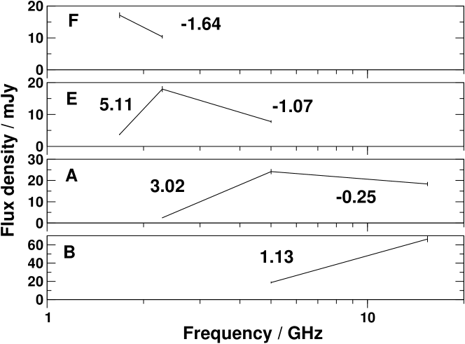
?figurename? 5.3: Spectra of components in NGC 3079 with the spectral indices labelled. The turnover frequency of each component increases with decreasing right ascension, suggestive of a wedge-shaped absorber in front of the AGN. All spectral indices were calculated from the September 2002 data, except for $\alpha^{5.0}_{15.4}$ for component $A$ and $B$, which were calculated from the November 2000 data to avoid variability effects.

5.2.2 Proper Motion

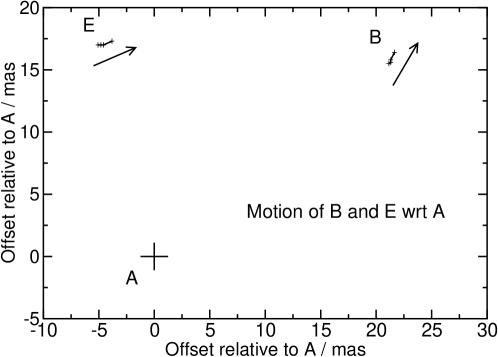
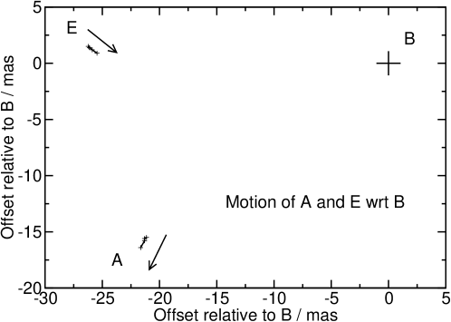
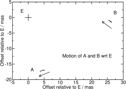
?figurename? 5.4: Relative positions among components $A$, $B$ and $E$ in NGC 3079 at 5.0 GHz for all epochs with arrows showing the direction of relative motion.

So far, the location of the AGN in NGC 3079 has not been accurately determined. Based on VLBI maser observations, Trotter et al. (1998) have suggested that the core lies on the $A-B$ axis, where that axis intersects the line of masers, and this identification has been supported by Sawada-Satoh et al. (2000) and, recently, by Kondratko (2003).

The relative positions of components $A$, $B$ and $E$ measured at 5.0 GHz are listed in Table 4.5 and are plotted in Fig. 5.4. In each plot, one component serves as a stationary reference point, and the arrows indicate in which direction the other two components are moving. The errors are $\sqrt{2}\times 0.15\,{\rm mas}=0.21\,{\rm mas}$, because the error of the reference point was added to the other errors.

A stationary

If $A$ is chosen as a stationary reference point, then $B$ is seen to move radially away from $A$, and $E$ is moving almost perpendicular to the $A-E$ axis. The motion of $E$ would not be expected in the standard AGN model, where radio components move radially away from the AGN. If $E$ was ejected by the AGN located at or near $A$, then its path must have a large bend that first makes it travel away from $A$ and then directs it in the same direction in which $B$ is travelling. We do not consider this scenario further.

B stationary

If $B$ is the reference, then $A$ is seen to move radially away from $B$, but $E$ is moving towards the $A-B$ axis. This situation, like the previous, does not agree very well with the standard model, in which one would not expect components to move in a direction away from the AGN. Nevertheless, this scenario is of particular importance. Sawada-Satoh et al. (2000), comparing their maser and continuum observations to those of Trotter et al. (1998), found $B$ to be stationary with respect to the brightest maser features. In this case, plotting the separations relative to $B$ yields the same speeds and directions as plotting them relative to the masers and hence to the true (radio-invisible) AGN centre of mass location, and $E$ would indeed be moving in the direction of the nucleus. Furthermore, Kondratko (2003) recently found good evidence for a rotating disc centred on the $A-B$ axis, confirming those results.

E stationary

If $E$ is the reference, then $A$ and $B$ move in almost perpendicular directions. This scenario has one attractive advantage, namely that the back-extrapolation of the trajectories of $A$ and $B$ intersect in the past. This allows them to be ejected from the same location, south-west of $B$. $E$ could be an object that is kinematically disconnected from the nucleus and is not part of the AGN ejecta. An obvious guess is to identify it as a supernova, supported by the fact that $E$ has not been observed by Trotter et al. (1998) in 1992, but was detected by Sawada-Satoh et al. (2000) in 1996, although they misidentified it with $B$. Thus, $E$ must have appeared between 1992 and 1996. At 5.0 GHz, it has an average flux density of 4.89 mJy, corresponding to $1.3\times 10^{20}\,{\rm W\,Hz^{-1}}$ at a distance of 15 Mpc. This is comparable to the brightest supernova in, e.g., M82, $41.9+58$, having $4.6\times 10^{19}\,{\rm W\,Hz^{-1}}$ at 5 GHz (Kronberg et al. 1985), although most of the supernovae reported in that publication have ten times lower luminosity. However, $E$ lacks the typical decrease in flux density that is seen as the supernova shells expand. Although Sawada-Satoh et al. (2000) find a flux density of $(5.7\pm 1.7)\,{\rm mJy}$ at 1.4 GHz, compared to $(3.06\pm 0.15)\,{\rm mJy}$ in our 1.7 GHz observations, the integrated flux densities were $(4.15\pm 0.21)\,{\rm mJy}$, $(3.08\pm 0.15)\,{\rm mJy}$, $(5.20\pm 0.26)\,{\rm mJy}$ and $(7.11\pm 0.36)\,{\rm mJy}$ in our 5.0 GHz observations. This sequence of measurements does not suggest a gradual decline of flux density with time like has been observed in M82’s $41.9+58$ during 1971-1981, fading with a rate of between $9\,\%\,{\rm yr^{-1}}$ and $24\,\%\,{\rm yr^{-1}}$ (Kronberg et al. 1985).

Core invisible

It is also possible that none of the radio emitters is coincident with the dynamical centre. This situation is common in radio galaxies and quasars where one usually sees a $\tau=1$ surface in the jet, and not a component at the location of the black hole, but as a Seyfert 2 galaxy, NGC 3079 is certainly an entirely different object. If the dynamical centre is invisible in the radio, the components may be shocks in an AGN outflow.

Helical paths

Another interesting interpretation is that all components are moving on paths that follow a helix with a fairly wide opening angle. If the axis of the helix is inclined at a small angle to the line of sight, inwards motion of components would be easily explained.

None of the five scenarios sketched above yields compelling evidence for the location of the core. However, we think that the model in which $B$ is stationary (it might be equivalent to the model in which the core is invisible) and the helical paths model need to be considered in the future. Maser observations are usually regarded as one of the “best possible” pieces of evidence for the location of black holes in AGN, but the kinematic centres of circumnuclear discs do not necessarily need to coincide with these cores. This has been found in, e.g., NGC 4261 (Ferrarese et al. 1996, see §3.3), although in that case, the multiple centres are interpreted as being due to past merging events, and spiral galaxies like NGC 3079 are generally not considered as descendants of galaxy mergers. We plan to monitor NGC 3079 during the next two years using phase-referencing with good frequency coverage between 1.7 GHz and 22 GHz, allowing us to follow absolute proper motions to resolve the ambiguous findings and solve for the core position.

5.2.3 Remarks on Individual Components

Component $A$ is the most compact component in NGC 3079. The ratio of peak flux density to integrated flux density, $x$, has an average of $0.85$ when measured from tapered images and of $0.69$ when measured from the full resolution images from November 1999, March 2000 and November 2000 (Table 4.3). Hence, it is only slightly resolved.

Component $B$ is clearly resolved at 5.0 GHz in the first three epochs ($x=0.39$) and compact at 15 GHz ($x=0.83$). This is probably not a resolution effect because the 5.0 GHz and 15 GHz images have similar resolution (the 15 GHz resolution even being slightly smaller), but a combination of steep spectral index and lower sensitivity can in principle account for the effect. The extension of $B$ to the south in the 5.0 GHz images has four to five contours, the lowest contour being drawn at three times the image rms. The extension therefore has a surface brightness of 8 to 16 times $3\,\sigma$, which is of the order of $1.6\,{\rm mJy\,beam^{-1}}$ to $3.2\,{\rm mJy\,beam^{-1}}$. Assuming a spectral index of $-0.7$ as is common for optically thin synchrotron radiation then predicts a surface brightness at 15.4 GHz of $0.7\,{\rm mJy\,beam^{-1}}$ to $1.5\,{\rm mJy\,beam^{-1}}$. This is visible as an extension of the lowest contour in the 15 GHz images which are drawn at around $1\,{\rm mJy\,beam^{-1}}$, especially in the November 2000 epoch, where this contour is at $0.82\,{\rm mJy\,beam^{-1}}$. Furthermore, Kondratko (2003) finds the same extension of $B$ at 22 GHz to have a surface brightness of $({\rm 0.42\leavevmode\nobreak\ to\leavevmode\nobreak\ 0.84)\,mJy\,beam^{-1}}$, consistent with a similar extrapolation of the surface brightness found by us at 5.0 GHz. Thus, the northern and compact part of $B$ has an inverted spectrum between 5.0 GHz and 15.4 GHz, whereas the extension to the south fades towards higher frequencies. If these two different spectral shapes on such small linear scales are interpreted as being due to free-free absorption, the situation does not agree well with the idea of a single, wedge-shaped absorber in front of the radio components as suggested in §5.2.1. But there are too few observational constraints to conclusively tell what causes the spectral gradient in $B$.

Component $E$ is also resolved, with an average peak-to-integrated ratio of 0.30 in the full-resolution images. Furthermore, the position angle of its largest extent appears to change between the first three epochs. We have fitted elliptical Gaussians to the $(u,v)$ data of all 5.0 GHz epochs, using data with a $(u,v)$ radius of $<100\,{\rm M\lambda}$ during the first three epochs and using data with a $(u,v)$ radius of $<50\,{\rm M\lambda}$ of the fourth epoch. The limits were chosen to reduce the ellipticity of the $(u,v)$ coverages while keeping as many data as possible. The results of the fits are listed in Table 5.5. The P.A. changes between the first three epochs are $28.7^{\circ}$ and $55.8^{\circ}$, whereas the P.A. change between the November 2000 and September 2002 epochs is difficult to determine due to the $n\pi$ ambiguity of the P.A. However, the rates at which the P.A. changed is $97.2^{\circ}\,{\rm yr^{-1}}$ between November 1999 and March 2000 and $76.3^{\circ}\,{\rm yr^{-1}}$ between March 2000 and November 2000. Extrapolating over the 1.811 yr period between the third and fourth epoch yields P.A.s of $231.8^{\circ}$ ($\mathrel{\widehat{=}}51.8^{\circ}$ when the P.A.s are reflected onto the range $0^{\circ}$ to $180^{\circ}$) for a rate of $97.2^{\circ}\,{\rm yr^{-1}}$ and $269.8^{\circ}$ ($\mathrel{\widehat{=}}89.8^{\circ}$) for a rate of $76.3^{\circ}\,{\rm yr^{-1}}$, or an average P.A. of $70.8^{\circ}$. This is very close to the observed P.A. of $65.0^{\circ}$.

However, we deem this result not very reliable. First, the P.A.s changed considerably when the maximum $(u,v)$ radius in imaging was changed and second, the P.A.s predicted for the September 2002 observation, $51.8^{\circ}$ and $89.8^{\circ}$, span $38.0^{\circ}$, and hence there is a probability of $100\times(38.0^{\circ}/180^{\circ})=21\,\%$ of the measured P.A. falling into that range if it was random. The P.A. changes of $E$ are not the result of a changing $(u,v)$ coverage, as the restoring beam after tapering the images is independent of the P.A. of $E$.

Combining this result with the observed spectra and proper motion, we find the least exotic explanation for the radio emission of component $E$ is an evolving shock in a large jet-like outflow.

	Beam size of image			Size of $E$
Epoch	$b_{\rm maj}$	$b_{\rm min}$	PA($b_{\rm maj}$)	$b_{\rm maj}$	$b_{\rm min}$	PA($b_{\rm maj}$)
	mas	mas	deg	mas	mas	deg
Nov 1999	2.69	2.20	-18.3	2.50	1.42	9.2
Mar 2000	1.85	1.68	-29.6	2.09	1.17	37.9
Nov 2000	2.35	1.86	-24.8	2.32	1.57	93.7
Sep 2002	4.16	3.81	-50.6	2.28	2.07	65.0

?tablename? 5.5: Position angle changes of component $E$.

5.3 Statistics

We have carried out a literature review to compare the findings in NGC 3079 to other Seyfert galaxies and AGN to address the following questions.

• The spectral indices of the radio components in NGC 3079 were found to be unusually inverted. Is this peculiar to NGC 3079 or do other Seyferts have inverted spectra as well? The result might indicate whether free-free absorption is common in Seyferts or not.

• NGC 3079, like some other Seyferts, shows a kpc-scale outflow, and if pc-scale components tend to be ejected in the same direction, this could help in the identification of components in NGC 3079. Is there a general correlation between the host galaxy rotation axes in Seyferts and the pc-scale emission? This might indicate that Seyfert radio ejecta are undergoing significant interactions with interstellar gas, or precession in the accretion discs, whereas powerful objects frequently are aligned from the innermost regions to the outer radio lobes.

• How do the VLBI-measured spectral indices in Seyferts generally compare to those measured with smaller arrays?

5.3.1 Compilation of the Sample

The range of radio properties displayed by Seyfert galaxies has been explored extensively based on WSRT, VLA or ATCA observations at 1.4 GHz, 5 GHz or 8.4 GHz at arcsec resolution by de Bruyn & Wilson (1978), Ulvestad & Wilson (1984, 1989), Unger et al. (1987), Giuricin et al. (1990), Rush et al. (1996), Nagar & Wilson (1999), Morganti et al. (1999), Ulvestad & Ho (2001a), and Vir Lal (2001). They studied the range of radio luminosities, radio source sizes, morphologies, alignment between jet and host galaxy, and spectral indices, and looked for dependence of properties on Seyfert type. With the exception of Ulvestad & Ho (2001a), who found 50 % of low-luminosity Seyferts to have a flat spectrum core, they all found that most Seyfert galaxies have steep, optically-thin synchrotron radio spectra, with 5 % to 35 % (depending on the sample) showing a flat-spectrum core, much less than the rate of occurrence of flat-spectrum cores in powerful radio galaxies. No difference was found between the spectral index distributions of the two Seyfert types.

However, the $0.3^{\prime\prime}$ to several arcsec beams used in those studies do not allow details of nuclear structure to be separated or the distribution of jet bending angles to be constructed. Further, they would probably blend together multiple radio components within the nucleus and could hide the presence of more absorbed cores.

Many further VLBI observations of Seyfert galaxies are available in the literature but no statistical summary from those observations has been presented. Thus, we made a literature search for VLBI observations of Seyferts to compare to our observations of NGC 3079. The resulting list in Table LABEL:tab:seyferts contains, we believe, all VLBI imaging observations of AGN classified as Seyfert 1, 2 or 3 by Véron-Cetty & Véron (2001) (irrespective of any sub-classification), published as of August 2003 with a linear resolution of $<10\leavevmode\nobreak\ {\rm pc}$, although it is not impossible that we have inadvertently omitted some works. This sample consists mostly of the nearest and best-known Seyferts. They were often selected for observing because they show bright radio nuclei at arcsecond resolution, and so the sample is not complete in any sense. Large, uniform samples of Seyfert galaxies are being observed with the VLBA by Murray et al. (1999) and Schmitt et al. (2002), but the results are not yet available. Proper motions in Seyferts are being presented by Roy et al. (in prep.) and we confine ourselves here to spectral indices and jet bending.

Spectral indices have been taken from the literature if they were measured simultaneously between L-band and C-band, i.e., between 1.4 GHz to 1.7 GHz and 4.9 GHz to 5.0 GHz. To compare pc and kpc-scale structure, we have searched for interferometric radio observations with a linear resolution of $>100\,{\rm pc}$, made with, e.g., the VLA or MERLIN. The angles have been measured from the images by us, from the identified core or the brightest component to the next bright component. The complete list is shown in Table LABEL:tab:seyferts, those objects used for determining spectral indices are listed in Table 5.7, and the angles are shown in Table LABEL:tab:seyferts_angles. We have plotted the data in two histograms shown in Fig. 5.5.

5.3.2 Spectral Properties of Seyferts

We selected from Table LABEL:tab:seyferts a subsample consisting of the Seyfert galaxies for which dual-frequency VLBI observations have been made to study the component spectral properties at high resolution. This subsample is listed in Table 5.7 and includes the spectra of $A$, $B$ and $E$ in NGC 3079 .

Spectral Index Distributions

The distribution of $\alpha^{1.4}_{5}$ from Table 5.7 is shown in Fig. 5.5 (top). The spectral indices lie between $-1.8$ and $+4.6$ with a median of $-0.40$ (using the Kaplan-Meier estimator constructed by ASURV rev 1.2, Lavalley et al. 1992 to account for lower limits and discarding upper limits). The distribution shows a tail towards positive spectral index due to four components in NGC 1068, NGC 2639 and NGC 3079 that have strong low-frequency absorption.

Separating the VLBI measurements by Seyfert type, we found the median $\alpha^{1.4}_{5}$ for the Sy 1s was $-0.75$ and for the Sy 2s was $-0.23$, which were not significantly different under the survival analysis two-sample tests ($P=6\,\%$ to $12\,\%$ that the spectral-index distributions came from the same parent distribution) or under a Kolmogorov-Smirnov test ($P=6\,\%$ to come from the same parent distribution), treating only lower limits as detections.

Despite the statistical insignificance of a difference between Seyfert types, we notice that the most inverted spectra all occur in objects that have evidence for an absorber. NGC 3079 has good evidence for free-free absorption, NGC 1068 and Mrk 348 are type 2 Seyferts with type 1 spectra in polarized light and NGC 2639 shows strong X-ray absorption (Wilson et al. 1998). The inner edge of such an absorber is expected to be ionized by UV emission from the AGN which would produce free-free absorption and hence produce inverted spectra preferentially in the type 2s. All four objects with inverted radio spectra also host ${\rm H_{2}O}$ masers, which is also consistent with an orientation effect if, for example, the radio core is viewed through a molecular disc or torus, which produces ${\rm H_{2}O}$ maser emission.

With spectral indices of $\alpha^{1.4}_{5}(A)>4.56$, $\alpha^{1.4}_{5}(B)>4.41$ and $\alpha^{1.4}_{5}(E)=0.67$, NGC 3079 has contributed the two most inverted spectra seen in any Seyfert on parsec scales. However, many more radio components in Seyferts have flat or inverted spectra, and NGC 3079 seems to be an extreme object, possibly because it is an edge-on spiral galaxy and so there is more absorbing gas in the line of sight than in face-on Seyferts.

Spectral Indices Measured with Smaller Arrays

The tail of extreme positive spectral indices that we see in our sample is not seen at arcsec resolution in the works mentioned in §5.3.1, probably due to component blending. We made a statistical comparison of our VLBI spectral indices to arcsec resolution spectral indices using the Kolmogorov-Smirnov test and chi-squared homogeneity test by treating the lower and upper limits as detections, and by applying survival analysis two-sample tests. The results are summarized in Table 5.8. Our spectral index distribution was significantly different (i.e. level of significance was less than the critical value of 5 %) from all the comparison samples according to all tests performed, with the exception of the Palomar Seyferts by Ho & Ulvestad (2001), which was found to be significantly different in only the chi-squared test. This excess of flat-spectrum sources in the Palomar Seyfert sample was already noticed by Ho & Ulvestad (2001).

Fraction of Flat-Spectrum Components

Of the 16 objects in the subsample, a majority of 13 (81 %) has at least one flat or inverted spectrum VLBI component with $\alpha^{1.4}_{5}>-0.3$ (denoted by an asterisk in Table 5.7). This fraction is 60 % larger than that measured at lower resolution by Ho & Ulvestad (2001) for the Palomar Seyferts and four or more times larger than the fraction measured at arcsec resolution for the other samples (Table 5.9). The difference is highly significant for most samples, having a probability of $<0.1\,\%$ of occurring at random. The larger fraction of flat- and inverted-spectrum components found with VLBI is not unexpected since increasing resolution reduces the component blending.

Summary

Flat- or absorbed- spectrum cores are present in 13 of 16 Seyfert galaxies. The most strongly absorbed components tend to be in objects that also show other evidence for absorption, such as water maser emission or large X-ray absorption columns. In those cases, according to the Seyfert unification schemes, the flat-spectrum components would be viewed through an edge-on obscuring disc or torus, the ionized inner edge of which could be causing free-free absorption. If so, the situation in those objects is different from the Blandford-Königl jet model. However the case for free-free absorption is unambiguous in only NGC 3079 for which spectral indices are $>+2.5$. The other 12 Seyferts have $-0.3<\alpha<+2.5$ and so spectral turnovers could be produced by either synchrotron self-absorption or free-free absorption.

5.3.3 Jet Misalignment

Kiloparsec-scale linear radio structures in Seyfert galaxies are thought to be energized by jets or outflows originating at the AGN core, and so one might expect pc and kpc-scale radio structures to be aligned. Misalignments could be caused by changes in the ejection axis or by pressure gradients in the ISM. To look for such effects, we compiled kpc-scale radio observations of the VLBI Seyfert sample, where available. The resulting sample of 21 objects in Table LABEL:tab:seyferts_angles is, we believe, a complete list of Seyferts with both pc-scale and kpc-scale observations published, although seven of these objects either have no clear extended structure on one of the scales or the structure was deemed to be affected by processes on scales $>1\,{\rm kpc}$, e.g., buoyancy forces that are unrelated to changes in the jet ejection axis. In one object, NGC 1167, the double-sided kpc-scale emission is bent, so we quote both. This sample has a large overlap with the sample in Table LABEL:tab:seyferts_angles and, likewise, is not complete. Biases such as selection for bright radio nuclei are probably present, but whether they affect the distribution of jet bending angle is unclear. Doppler boosting would favour jets that point towards us, but the jet speeds so far measured in Seyferts are low and boosting effects should be minor.

The distribution of misalignment angles from Table LABEL:tab:seyferts_angles is shown in Fig. 5.5 (bottom). Misalignment in Seyfert jets between pc and kpc-scales is common, with 5 out of 15 objects bending by $45^{\circ}$ or more. The null hypothesis that the jet bending-angle distribution was drawn from a parent population of aligned jets was rejected by a chi-squared test at the 2 % level of significance. The null hypothesis that the distribution was drawn from a uniformly distributed parent population could not be rejected by a chi-squared test, which returned a 25 % level of significance. Thus, the misalignment between the pc-scale and kpc-scale radio structure in NGC 3079 is common in Seyfert galaxies.

The frequent misalignments seen in Seyfert galaxy jets could be evidence either for changes in the jet ejection angle and hence of the accretion disc, perhaps by a mechanism such as radiation-driven warping (Pringle 1997), or for bending due to pressure gradients in the ISM (collision or buoyancy) through which the jets propagate.

We compared the extended pc-scale radio structures to the host galaxy rotation axes, assuming that the host galaxy is circular and the rotation axis vector is projected onto the galaxy’s minor axis, which can be measured from optical images. For all spiral galaxies with pc-scale radio structure, we used the major axes from de Vaucouleurs et al. (1991), subtracted $90^{\circ}$ and reflected the angles onto the range $0^{\circ}$ to $90^{\circ}$. Four objects were not listed in de Vaucouleurs et al. (1991), so we used data from Schmitt & Kinney (2000) in two cases and we measured the major axes from Hubble Space Telescope archival data in the other two cases. We performed a Spearman rank correlation test and found a correlation coefficient of 0.07, corresponding to a 82 % significance and so there is no correlation between the directions of the pc-scale structures and the host galaxy rotation axes. However, the sample was small (13 objects) and therefore the test is not strong. Thus, the lack of alignment in Seyferts between pc-scale and kpc-scale structure does not allow one to identify a pc-scale ejection axis in NGC 3079. Precession of the ejection axis is common and may be reflected in the confusing structure in the core of NGC 3079.

We compared the bending angles in Seyferts to those in radio-loud objects using a comparison sample of core-dominated radio-loud objects compiled from Table 6 in Pearson & Readhead (1988), and Table 1 in Conway & Murphy (1993), which have both VLBI and VLA or MERLIN observations at 5 GHz. Those objects show a surprising bimodal distribution of jet bending angle, in which the pc-scale jets tend to align with or to be perpendicular to the kpc-scale structure. We compared our jet bending angle distribution to the distribution in radio-loud objects using a Kolmogorov-Smirnov test and found no significant difference, the probability of being drawn from the same parent distribution being 14 %. However, the Seyfert sample is small and the distribution for the Seyferts was shown in the previous paragraph to be consistent also with a uniform distribution.

Summary

The position angle differences between pc-scale and kpc-scale radio emission were found to be uniformly distributed between $0^{\circ}$ and $90^{\circ}$. Such bends could be due to changes in the jet ejection axis or due to pressure gradients in the ISM. No correlation was found between the axis of pc-scale radio structure and the rotation axis of the host galaxy.

We conclude that NGC 3079 shares most properties with other Seyferts. Its spectra are extreme, but three other objects also showed inverted spectra and the transition between these three and NGC 3079 does not appear to mark a fundamental difference, and misalignment between pc-scale and kpc-scale radio emission also is a common finding.

?tablename? 5.6: Seyferts observed with VLBI. Column 1 lists the names we used, column 2 the names used by Véron-Cetty & Véron (2001), column 3 the Seyfert types as described by Véron-Cetty & Véron (2001) , column 4 the linear resolution in pc, column 5 the instrument and frequency used, and column 6 the reference to the publication.

Name	Véron name	Class	Lin. Res.	Instrument	Ref.
3C 287.1		S1	5.43	VLBA 5 GHz	Fomalont et al. (2000)
3C 390.3		S1.5	1.09	global VLBI 5 GHz	Alef et al. (1996)
III Zw 2		S1.2	0.260	VLBA 15/43 GHz	Brunthaler et al. (2000)
Ark 564		-	0.598	global VLBI 5 GHz	Vir Lal (2001)
IC 5063	PKS 2048-57	S1h	3.30	LBA 2.3 GHz + LBA HI	Oosterloo et al. (2000)
MCG 8-11-11		S1.5	0.635	global VLBI 5 GHz	Vir Lal (2001)
Mrk 1		S2	6.18	EVN 1.7 GHz	Kukula et al. (1999)
Mrk 1		S2	0.550	global VLBI 5 GHz	Vir Lal (2001)
Mrk 3		S1h	5.24	EVN 1.7 GHz	Kukula et al. (1999)
Mrk 78		S2	1.75	global VLBI 5 GHz	Vir Lal (2001)
Mrk 231		S1.0	0.343	VLBA 15 GHz	Ulvestad et al. (1999b)
Mrk 231		S1.0	4.09	VLBA 1.4/2.3/4.8/8.4/15/22 GHz	Ulvestad et al. (1999a)
Mrk 273		S2	7.32	VLBA 1.4 GHz	Carilli & Taylor (2000)
Mrk 348		S1h	0.131	VLBA 15 GHz	Ulvestad et al. (1999b)
Mrk 348		S1h	6.41	EVN 1.4 GHz	Neff & de Bruyn (1983)
Mrk 348		S1h	1.49	VLBA 1.7/5.0/8/15/22 GHz	Peck et al. (2003)
Mrk 477		S1h	2.39	global VLBI 5 GHz	Vir Lal (2001)
Mrk 530	NGC 7603	S1.5	1.45	global VLBI 5 GHz	Vir Lal (2001)
Mrk 766		S1.5	0.413	global VLBI 5 GHz	Vir Lal (2001)
Mrk 926		S1.5	0.917	VLBA 8.4 GHz	Mundell et al. (2000)
Mrk 1210		S1h	0.392	EVN 1.6/5 GHz VLBA 1.6/5 GHz	Middelberg et al. (2004)
Mrk 1218		S1.8	0.582	global VLBI 5 GHz	Vir Lal (2001)
NGC 1052		S3h	0.015	VLBA 5/8.4/22/43 GHz	Kadler et al. (2002)
NGC 1052		S3h	0.048	VLBI 1.4-43.2	Vermeulen et al. (2003)
NGC 1052		S3h	0.038	VLBA 2.3/8.4/15.4 GHZ	Kameno et al. (2001)
NGC 1068		S1h	0.221	VLBA 1.7,5,15 GHz	Roy et al. (1998)
NGC 1068		S1h	2.94	EVN 1.4 GHz	Ulvestad et al. (1987)
NGC 1167		S3	0.895	global VLBI 5 GHz	Giovannini et al. (2001)
NGC 1167		S3	0.639	global VLBI 1.6 GHz	Giovannini et al. (1990)
NGC 1275		S1.5	0.416	VLBA 2.3/5/8.4/15.4/22/43 GHz	Walker et al. (2000)
NGC 2110		S1i	0.151	VLBA 8.4 GHz	Mundell et al. (2000)
NGC 2110		S1i	0.966	EVN 1.6/5 GHz	Middelberg et al. (2004)
NGC 2273		-	0.342	global VLBI 5 GHz	Vir Lal (2001)
NGC 2639		S3	0.233	global VLBI 5 GHz	Vir Lal (2001)
NGC 2639		S3	0.162	VLBA 1.6/5/15 GHz	Wilson et al. (1998)
NGC 3079		S2	0.044	VLBA 5/8/22 GHz	Trotter et al. (1998)
NGC 3079		S2	0.054	global VLBI, 5.0 GHz	Irwin & Seaquist (1988)
NGC 3079		S2	0.042	global VLBI 1.4/8.4/15/22	Sawada-Satoh et al. (2000)
NGC 3147		S2	0.219	VLBA 1.6/2.3/5/8.4 GHz	Ulvestad & Ho (2001b)
NGC 3227		S1.5	3.74	MERLIN 1.6/5 GHz	Mundell et al. (1995)
NGC 4151		S1.5	0.116	VLBA 1.6,5 GHz	Ulvestad et al. (1998)
NGC 4151		S1.5	1.29	EVN 1.7 GHz	Harrison et al. (1986)
NGC 4151		S1.5	4.82	MERLIN 5 GHz	Pedlar et al. (1993)
NGC 4168		S1.9	0.236	VLBA 5 GHz	Nagar et al. (2002)
NGC 4203		S3b	0.084	VLBA 1.6/2.3/5/8.4 GHz	Ulvestad & Ho (2001b)
NGC 4258		S2	0.029	VLBA 22 GHz	Herrnstein et al. (1997)
NGC 4258		S2	0.232	VLBA 1.4/1.6 GHz	Cecil et al. (2000)
NGC 4395		S1.8	0.221	VLBA 1.4 GHz	Wrobel et al. (2001)
NGC 4565		S1.9	0.207	VLBA 5 GHz	Falcke et al. (2000)
NGC 4579		S3b	0.118	VLBA 1.6/2.3/5/8.4 GHz	Ulvestad & Ho (2001b)
NGC 4579		S3b	0.246	VLBA 5 GHz	Falcke et al. (2000)
NGC 5252		S2	0.671	VLBA 8.4 GHz	Mundell et al. (2000)
NGC 5506		S1i	0.815	EVN 1.6/5 GHz	Middelberg et al. (2004)
NGC 5548		S1.5	0.366	VLBA 8.4 GHz	Wrobel (2000)
NGC 5793		S2	0.135	VLBA 1.7,8.4,15,22 GHz	Hagiwara et al. (2001)
NGC 5793		S2	0.316	VLBA+Y27 1.6/5 GHz	Hagiwara et al. (2000)
NGC 5929		S3	0.290	global VLBI 5 GHz	Vir Lal (2001)
NGC 5929		S3	6.44	MERLIN 0.4/1.6/5	Su et al. (1996)
NGC 7212		S1h	1.37	global VLBI 5 GHz	Vir Lal (2001)
NGC 7469		S1.5	0.844	global VLBI 5 GHz	Vir Lal (2001)
NGC 7674		S1h	2.80	VLBA+Y27+Arecibo 1.4 GHz	Momjian et al. (2003)
NGC 7674		S1h	2.58	EVN 1.6/5 GHz	Middelberg et al. (2004)
NGC 7674		S1h	2.18	global VLBI 5 GHz	Vir Lal (2001)
NGC 7682		S2	0.996	global VLBI 5 GHz	Vir Lal (2001)
T0109-383	NGC 424	S1h	0.226	VLBA 8.4 GHz	Mundell et al. (2000)

Source	Flat/Inv.	Comp.	$\alpha^{1.4}_{5}$	Refs.
Mrk 231	*	N	$-$0.86	Ulvestad et al. (1999a)
		C	$+$0.88	Ulvestad et al. (1999a)
		S	$-$1.54	Ulvestad et al. (1999a)
Mrk 348	*		$+$0.93	Barvainis & Lonsdale (1998)
Mrk 463E		L	$-$1.06	Norris et al., unpublished
		R	$-$0.62	Norris et al., unpublished
		1	$-$0.67	Norris et al., unpublished
		2	$-$0.77	Norris et al., unpublished
		3	$-$1.00	Norris et al., unpublished
Mrk 1210		NW	$-$1.26	Middelberg et al. (2004)
		SE	$-$0.78	Middelberg et al. (2004)
NGC 1068	*	NE	$-$1.5	Roy et al. (1998)
		C	$>2.2$	Roy et al. (1998)
		S1	$>0.6$	Roy et al. (1998)
		S2	$<-1.9$	Roy et al. (1998)
NGC 2110	*	C	$+0.12$	Middelberg et al. (2004)
NGC 2639	*		$+1.78$	Wilson et al. (1998)
NGC 3079	*	E	$+0.67$	This thesis
		A	$>+4.56$	This thesis
		B	$>+4.41$	This thesis
NGC 3147	*		$+0.20$	Ulvestad & Ho (2001b)
NGC 4151	*	E	$-0.5$	Ulvestad et al. (1998)
		D	$<-0.2$	Ulvestad et al. (1998)
		F	$<-1.3$	Ulvestad et al. (1998)
NGC 4203	*		$+0.38$	Ulvestad & Ho (2001b)
NGC 4579	*		$+0.20$	Ulvestad & Ho (2001b)
NGC 5506	*	B0	$+0.06$	Middelberg et al. (2004)
		B1	$-0.73$	Middelberg et al. (2004)
		B2	$-0.30$	Middelberg et al. (2004)
NGC 5793	*	C1C	$-0.70$	Hagiwara et al. (2000)
		C1NE	$-1.00$	Hagiwara et al. (2000)
		C2C	$-0.46$	Hagiwara et al. (2000)
		C2W	$-0.72$	Hagiwara et al. (2000)
		C2E	$+0.13$	Hagiwara et al. (2000)
NGC 7469	*	2	$-0.34$	Norris et al., unpublished
		3	$+0.09$	Norris et al., unpublished
		5	$-0.12$	Norris et al., unpublished
NGC 7674			$-1.78$	Middelberg et al. (2004)

?tablename? 5.7: Seyferts from Table LABEL:tab:seyferts that have dual-frequency (1.4 GHz and 5 GHz) VLBI observations with matching beam sizes, from which the spectral index is derived. Asterisks denote objects with at least one component with a flat or inverted spectrum.

		Level of Significance
Sample		$\chi^{2}$	KS	Logrank	Gehan	Peto-Peto
Unger et al. (1987)	X-ray Seyferts	0.3 %	0.7 %	0.3 %	8.3 %	8.3 %
Rush et al. (1996)	CfA Seyferts	0.1 %	0.1 %	0.0 %	0.5 %	0.5 %
Rush et al. (1996)	12 $\mu$m Seyferts	0.1 %	0.6 %	0.0 %	2.0 %	2.0 %
Morganti et al. (1999)	Distance Limited	0.1 %	0.3 %	0.0 %	1.2 %	1.2 %
Ho & Ulvestad (2001)	Palomar Seyferts	1.0 %	27 %	44 %	75 %	77 %
Ulvestad & Wilson (1984)	Distance Limited	0.1 %	0.3 %	0.0 %	0.7 %	0.7 %

?tablename? 5.8: Comparison of the spectral index distribution of the VLBI Seyfert sample to various other Seyfert samples. The level of significance gives the probability that the spectral index distribution of the comparison sample and the VLBI seyfert sample in this thesis were drawn from the same parent population.

Sample		$N_{\alpha>-0.3}$	$N_{\rm total}$	%	$P$
Middelberg et al. (2004)	own obs + lit search	17	38	45
Unger et al. (1987)	X-ray Seyferts	1	20	5	$0.3$ %
Rush et al. (1996)	CfA Seyferts	3	46	6.5	$<0.1$ %
Rush et al. (1996)	12 $\mu$m Seyferts	4	40	10	$<0.1$ %
Morganti et al. (1999)	Distance limited	13	60	22	$1.8$ %
Ho & Ulvestad (2001)	Palomar Seyferts	21	45	47	$50$ %
Ulvestad & Wilson (1984)	Distance limited	3	40	7.5	$<0.1$ %

?tablename? 5.9: Fraction of flat- and inverted-spectrum components in various Seyfert samples. The column ’$N_{\alpha>-0.3}$’ gives the number of components with spectral indices $\alpha>-0.3$ (i.e., components with flat or inverted spectra). The column ’$N_{\rm total}$’ gives the total number of components in each sample. The column % gives $(N_{\alpha>-0.3}/N_{\rm total})\times 100$. The column $P$ gives the level of significance from a comparison of the fraction of flat- and inverted-spectrum components in the VLBI sample of this thesis (limits treated as detections), to that of each comparison sample at arcsec resolution, using the difference-of-two-proportions test with Yates correction for continuity (e.g. Glanz 1992).

?tablename? 5.10: Subset of sources from Table LABEL:tab:seyferts for which both pc and kpc-scale structures have been observed. The misalignment angle, $\Delta\Theta$, is calculated as $\Theta({\rm pc})-\Theta({\rm kpc})$, and has then been reflected onto the range of $0^{\circ}$ to $90^{\circ}$. For the seven objects at the end of the table, either the P.A. information of the kpc scale structure was not completely reliable or was unavailable. The position angles of the galaxy minor axes in the last column were drawn from de Vaucouleurs et al. (1991), except for those marked $a$ taken from Schmitt & Kinney (2000) and those marked $b$ measured by us from Hubble Space Telescope archival images (see §5.3.3).

Name	Res.	$\Theta$ (pc)	$\Theta$ (kpc)	$\Delta\Theta$	Array	Refs.	$\Theta$ (opt.)
	(pc)	(deg)	(deg)	(deg)			deg
3C 390.3	1.09	323		0	global VLBI 5 GHz	Alef et al. (1996)
	1210		323		VLA 5 GHz	Alef et al. (1996)
Mrk 78	1.75	40		55	global VLBI 5 GHz	Vir Lal (2001)
	504		275		VLA 5 GHz	Vir Lal (2001)
Mrk 231	0.343	93		77	VLBA 15 GHz	Ulvestad et al. (1999b)	100
	3270		170		VLA 1.5/8.4/15 GHz	Ulvestad et al. (1999a)
Mrk 1218	0.582	330		13	global VLBI 5 GHz	Vir Lal (2001)	130b
	294		317		VLA 5 GHz	Vir Lal (2001)
NGC 1052	0.015	65		30	VLBA 5/8.4/22/43 GHz	Kadler et al. (2002)
	162		275		MERLIN 1.4 GHz	Kadler et al. (2003)
NGC 1068	0.221	11		29	VLBA 1.7,5,15 GHz	Roy et al. (1998)	160
	217		40		VLA 5 GHz	Ho & Ulvestad (2001)
NGC 1167	0.895	140	313	7	global VLBI 5 GHz	Giovannini et al. (2001)
	131		66	74	VLA 5 GHz	Sanghera et al. (1995)
NGC 1275	0.416	353		23	VLBA 2.3 to 43 GHz	Walker et al. (2000)
	382		150		VLA 1.4 GHz	Pedlar et al. (1990)
NGC 3079	0.044	125		65	VLBA 5/8/22 GHz	Trotter et al. (1998)	75
	310		60		VLA 1.4/4.9	Duric et al. (1983)
NGC 4151	0.116	257		3	VLBA 1.6,5 GHz	Ulvestad et al. (1998)	140
	104		80		VLA 5 GHz	Ho & Ulvestad (2001)
NGC 4258	0.029	3		8	VLBA 22 GHz	Herrnstein et al. (1997)	60
	125		355		VLA 1.5 GHz	Cecil et al. (2000)
NGC 7212	1.37	257		52	global VLBI 5 GHz	Vir Lal (2001)	133a
	609		25		VLA 5 GHz	Vir Lal (2001)
NGC 7469	0.844	28		35	global VLBI 5 GHz	Vir Lal (2001)	35
	193		353		VLA 5 GHz	Vir Lal (2001)
NGC 7674	2.80	274		22	VLBA+Y27+AO 1.4 GHz	Momjian et al. (2003)	64a
	178		296		MERLIN 1.7	Momjian et al. (2003)
III Zw 2	0.260	303		63	VLBA 15/43 GHz	Brunthaler et al. (2000)
	3460		240		VLA 1.5 GHz	Brunthaler, priv. comm.
Ark 564	0.598	282			global VLBI 5 GHz	Vir Lal (2001)	28
IC 5063	3.30	66		49	LBA 2.3 GHz + LBA HI	Oosterloo et al. (2000)
	242		115		ATCA 8.3/1.4GHz	Morganti et al. (1998)
NGC 2110	0.151	350		16	VLBA 8.4 GHz	Mundell et al. (2000)
	240		186		VLA 1.4/5 GHz	Ulvestad & Wilson (1983)
NGC 3147	0.219	317			VLBA 1.6/2.3/5/8.4 GHz	Ulvestad & Ho (2001b)	65
NGC 5506	0.815	73		76	EVN 1.6/5 GHz	Middelberg et al. (2004)	1
	359		177		VLA 4.9 GHz	Colbert et al. (1996)
NGC 7682	0.996	125			global VLBI 5 GHz	Vir Lal (2001)	68b

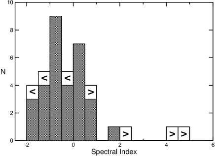
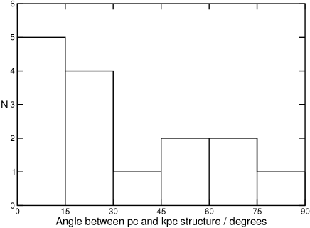
?figurename? 5.5: Histograms of Seyfert galaxy literature data. Top: Histogram of spectral indices with a bin width of 0.5. Bottom: Histogram of angles between pc and kpc-scale structure with a bin width of $15^{\circ}$.

?chaptername? 6 Fast Frequency Switching

The invention of Very Long Baseline Interferometry was mainly driven by the need for higher angular resolution radio observations. Single-dish observations would never have approached the resolutions achieved by optical telescopes owing to the long wavelengths. However, once VLBI was available, it was straightforward to progressively increase the resolution by increasing the observing frequencies. In the recent few years, observations at 86 GHz have evolved from the experimental stage to a commonly used observing technique which achieves the highest angular resolutions possible today, and first detections at even higher frequencies have already been made (Krichbaum et al. 2002). The scientific benefits are undoubted: even in the closest objects, only millimeter-VLBI can resolve the linear scales on which extragalactic radio jets are launched, a process yet not understood. 86 GHz VLBI observations also contribute to investigations of internal jet structure, composition and collimation (e.g., Doeleman et al. 2001, Gómez et al. 1999).

Unfortunately, higher frequency observations involve a number of serious problems: the sources are usually weaker because the emissivity of optically thin synchrotron sources drops as $\nu^{-0.7}$, the efficiencies of typical centimetre radio antennas drop to about 15 % because the surface rms is $\approx\lambda/10$, the receiver performances become disproportionately worse because the amplifiers contribute more noise and the atmospheric coherence that limits the integration time decreases as $1/\nu$. This last problem, however, is not a hardware property and would be solved if the atmospheric phase fluctuations could be calibrated. In fact, the so-called phase-referencing first demonstrated by Alef (1988) is now an established calibration technique in centimetre VLBI to lower the detection thresholds to the sub-mJy level and to accurately determine the positions of sources in VLBI observations. In phase-referencing, a strong calibrator source is frequently observed (every few minutes, depending on observing frequency) to calibrate the visibility phases of the target source integrations, i.e., the telescopes cycle between the target source and the phase calibrator source. In millimetre VLBI the technique is not commonly used, although a successful proof of concept exists (Porcas & Rioja 2002). Problems arise from the need of a suitable, strong phase calibrator in the vicinity of target source and from a combination of short atmospheric coherence and telescope slewing times.

In this chapter, I describe a new phase-referencing technique for VLBI observations at high frequencies, fast frequency switching.

6.1 Introduction

The main source of phase noise in VLBI observations at frequencies higher than 5 GHz is turbulence in the troposphere causing refractive inhomogeneities. These path-length variations are non-dispersive, and one can self-calibrate the visibility phases at one frequency and use the solutions to calibrate visibilities at another frequency after multiplying the phases by the frequency ratio, $r$, provided that the lag between the two measurements does not exceed half the atmospheric coherence time (Fig. 6.1). This is possible with the VLBA because frequency changes need only a few seconds. After multiplying the phase solutions by the frequency ratio and applying them to the target-frequency phases, there remains a constant phase offset, $\Delta\Phi$, between the signal paths at the two frequencies, which must be calibrated. It can be monitored with frequent observations of achromatic, strong calibrators, and must be subtracted from the high frequency visibility phase.

Following the notation from Eqs. 2.4ff, the observed visibility phases using this calibration scheme can be described as

$$\begin{split}\phi_{\rm\nu_{r}}(t_{1})&=\phi_{\rm r}(t_{1})+\phi_{\rm ins}^{\rm\nu_{r}}(t_{1})+\phi_{\rm pos}^{\rm\nu_{r}}(t_{1})+\phi_{\rm ant}^{\rm\nu_{r}}(t_{1})+\phi_{\rm atm}^{\rm\nu_{r}}(t_{1})+\phi_{\rm ion}^{\rm\nu_{r}}(t_{1})\\ \phi_{\rm\nu_{t}}(t_{2})&=\phi_{\rm t}(t_{2})+\phi_{\rm ins}^{\rm\nu_{t}}(t_{2})+\phi_{\rm pos}^{\rm\nu_{t}}(t_{2})+\phi_{\rm ant}^{\rm\nu_{t}}(t_{2})+\phi_{\rm atm}^{\rm\nu_{t}}(t_{2})+\phi_{\rm ion}^{\rm\nu_{t}}(t_{2})\\ \phi_{\rm\nu_{r}}(t_{3})&=\phi_{\rm r}(t_{3})+\phi_{\rm ins}^{\rm\nu_{r}}(t_{3})+\phi_{\rm pos}^{\rm\nu_{r}}(t_{3})+\phi_{\rm ant}^{\rm\nu_{r}}(t_{3})+\phi_{\rm atm}^{\rm\nu_{r}}(t_{3})+\phi_{\rm ion}^{\rm\nu_{r}}(t_{3}).\\ \end{split}$$ (6.1)

Here, the indices $\nu_{\rm r}$ and $\nu_{\rm t}$ denote terms of the reference and target frequency, respectively, and $\phi_{\rm r}$ and $\phi_{\rm t}$ are the true visibilities at the reference and target frequency, respectively. Interpolation of the reference frequency terms to the times of the target frequency scans yields

$$\tilde{\phi}_{\rm\nu_{t}}(t_{2})=\tilde{\phi}_{\rm r}(t_{2})+\tilde{\phi}_{\rm ins}^{\rm\nu_{r}}(t_{2})+\tilde{\phi}_{\rm pos}^{\rm\nu_{r}}(t_{2})+\tilde{\phi}_{\rm ant}^{\rm\nu_{r}}(t_{2})+\tilde{\phi}_{\rm atm}^{\rm\nu_{r}}(t_{2})+\tilde{\phi}_{\rm ion}^{\rm\nu_{r}}(t_{2}).$$ (6.2)

Self-calibration at the reference frequency is then used to obtain a source model, and self-calibration of the visibilities after dividing by this model yields the required phase corrections. These correction terms are interpolated to the times where the target frequency was observed, and scaled by the frequency ratio, $r$. In practice, the phase solutions derived in this process comprise contributions from all five sources of error, and so do the scaled phase corrections. The difference between the target frequency visibilities and the interpolated reference frequency visibilities then is

$$\begin{split}\phi_{\rm\nu_{t}}-\tilde{\phi}_{\rm\nu_{r}}=\phi_{\rm t}-\tilde{\phi}_{\rm r}&+(\phi_{\rm ins}^{\rm\nu_{t}}-r\tilde{\phi}_{\rm ins}^{\rm\nu_{r}})+(\phi_{\rm pos}^{\rm\nu_{t}}-r\tilde{\phi}_{\rm pos}^{\rm\nu_{r}})+(\phi_{\rm ant}^{\rm\nu_{t}}-r\tilde{\phi}_{\rm ant}^{\rm\nu_{r}})\\ &+(\phi_{\rm atm}^{\rm\nu_{t}}-r\tilde{\phi}_{\rm atm}^{\rm\nu_{r}})+(\phi_{\rm ion}^{\rm\nu_{t}}-r\tilde{\phi}_{\rm ion}^{\rm\nu_{r}}).\end{split}$$ (6.3)

In this equation, $\tilde{\phi}_{\rm r}$ is zero because a model of the source has been subtracted. The instrumental phase offset is constant and can be determined from calibrator observations, and so the term $(\phi_{\rm ins}^{\rm\nu_{t}}-r\tilde{\phi}_{\rm ins}^{\rm\nu_{r}})$ is known and can be removed. The antenna position errors also cancel out because this type of error causes a shift of the source on the sky, and to compensate for it requires a phase correction which scales with frequency. E.g., assume an antenna position error of 1 cm along the line of sight on a 1000 km baseline. The error shifts the fringe pattern on the sky by $(0.01\,{\rm m}/1000\,{\rm km})=10^{-8}\,{\rm rad}=2.06\,{\rm mas}$. At a frequency of 15 GHz ($\lambda=2.00\,{\rm cm}$), the fringe spacing on the sky is $\lambda/D=4.13\,{\rm mas}$, and hence a phase correction of $179^{\circ}$ is required to account for the error. At a frequency of 45 GHz ($\lambda=0.67\,{\rm cm}$), three times higher than the other frequency, the fringe spacing is 1.38 mas, and a phase correction of $537^{\circ}$ is required to compensate for the error, three times more than at the lower frequency, and so $(\phi_{\rm ant}^{\rm\nu_{t}}-r\tilde{\phi}_{\rm ant}^{\rm\nu_{r}})=0$. Similar to the antenna position error, the source position error scales with frequency when measured in units of turns of phase, but a frequency-dependent core shift, as predicted by conical jet models (e.g., Lobanov 1998), modulates $(\phi_{\rm pos}^{\rm\nu_{t}}-r\tilde{\phi}_{\rm pos}^{\rm\nu_{r}})$ on each baseline with a sinusoid. The period of the sinusoid is $23^{\rm h}56^{\rm m}$, its amplitude depends on the magnitude of the shift and its phase depends on the direction of the shift relative to the baseline direction. It is zero only in the abscence of a core shift, and therefore cannot be neglected. The atmospheric phase errors also scale with frequency, and hence $(\phi_{\rm atm}^{\rm\nu_{t}}-r\tilde{\phi}_{\rm atm}^{\rm\nu_{r}})=0$, but the ionospheric phase noise is difficult to determine; something which we, unfortunately, did not discover beforehand the observations presented here. It can probably be determined using interspersed, wide-band scans at a low frequency, e.g., in the 1.4 GHz band, where the effect is strong. Similar to Eq. 2.7, the remaining terms describe the difference between the target frequency phase and the interpolated reference frequency phase as the target frequency visibility phase plus the position offset and an interpolation term, $\phi_{\rm int}$:

$$\phi_{\rm\nu_{t}}-\tilde{\phi}_{\rm\nu_{r}}=\phi_{\rm t}+(\phi_{\rm pos}^{\rm\nu_{t}}-r\tilde{\phi}_{\rm pos}^{\rm\nu_{r}})+\phi_{\rm int}.$$ (6.4)

The result is the high-frequency visibilities phase-referenced to the source at low frequency, and so the technique can measure the position shift of AGN cores with frequency and can prolong coherence. The coherence time can in principle be prolonged indefinitely, however, in our project, unmodelled ionospheric path length changes limited the coherence to half an hour in the worst case. Thus, in the following sections, we use fast frequency switching to calibrate the short-term phase fluctuations and then use self-calibration at the target frequency with a half-hour solution interval to remove the long-term phase drifts. The extension from the 30 s atmospheric coherence time to a coherent integration time of 30 min yields a large sensitivity improvement.

A similar observing strategy has been developed by Kassim et al. (1993) for the VLA, who used scaled phase solutions from 330 MHz to calibrate simultaneously observed 74 MHz data. In this case, the dominant source of phase errors was ionospheric path length changes. Using their new calibration technique, they were able to increase the coherent integration time from $<$ 1 min to $>$ 10 min and to make 74 MHz images of several radio sources. Fast frequency switching is also being considered as a standard calibration mode for ALMA in the future (D’Addario 2003).

?figurename? 6.1: Demonstration of the scalability of phase solutions. 43 GHz fringe-fitted phase solutions (solid lines) on 3C 273 compared to 15 GHz fringe-fitted phase solutions multiplied by the frequency ratio (dashed lines) from Hancock (upper panel) and Kitt Peak (lower panel). Ten minutes of data are shown, and the phases follow each other very well.

6.2 Observations

We observed a pilot project (BR073) on January 5, 2002, to attempt to measure the diameter of the AGN in M81 (M81*) at 86 GHz. We obtained only very weak detections of M81*, but we learnt a number of important points about designing fast-frequency switching experiments (Middelberg et al. 2002). We incorporated those considerable improvements in the observing strategy for our next project (BM175C), which we describe here.

Source	Duration	Freq.	3C279	5	43
	(min)	pair	3C273	5	43
(1)	(2)	(3)	3C273	5	1
OJ287	10	15-86	NGC4261	25	15-43
OJ287	10	15-43	3C273	5	15-43
NGC4261	25	15-43	3C273	5	15-86
3C273	5	15-43	NGC4261	25	15-86
NGC4261	25	15-86	3C279	5	15-43
3C273	5	15-86	3C279	5	15-86
3C273	5	15-43
			3C273	10	15-43
OJ287	5	15a			15-
OJ287	5	43a	NGC4261	25	15-43
OJ287	5	86a	3C273	5	15-43
			3C273	5	15-86
NGC4261	25	15-43	NGC4261	25	15-86
3C279	5	15-43	3C279	5	15-86
3C279	5	15-86	3C279	5	15-43
3C273	5	15-86
3C273	5	15-43	3C279	5	15a
NGC4261	25	15-43	3C279	5	43a
3C273	5	15-43	3C279	5	86a
3C273	5	15-86
NGC4261	25	15-86	3C273	5	15-43
3C279	5	15-86	3C273	5	15-86
3C279	5	15-43	NGC4261	25	15-86
			3C273	5	15-86
3C273	10	15-43	3C273	5	15-43
			NGC4261	25	15-43
NGC4261	25	15-43	3C279	5	15-43
3C273	5	15-43	3C279	5	15-86
3C273	5	15-86	3C273	5	15-43
NGC4261	25	15-86
3C279	5	15-86	3C345	5	15a
			3C345	5	43a
3C279	5	15a	3C345	5	86a
3C279	5	43a
3C279	5	86a	3C345	10	15-43
			3C345	10	15-86

?tablename? 6.1: Summary of project BM175 observed on May 5, 2003. The sources observed are in column (1), the scan duration is in column (2) and the frequency pairs in GHz are in column (3). An $a$ indicates fringe finder scans during which no frequency switching was done.

We observed NGC 4261 as a fast frequency switching target and 3C 273 and 3C 279 occasionally for the inter-frequency offset and to test the technique on strong sources on May 5, 2003 (project BM175C). A previous run (BM175B) had to be re-observed because of high fringe rates due to weather and a number of equipment failures. BM175C was observed in a period of superb weather, using 256 Mbps to record a bandwidth of 64 MHz with 2-bit sampling. We recorded LCP only, the data were divided into 8 IFs with 8 MHz bandwidth, each of which were subdivided into 64 spectral channels 125 kHz wide. The correlator integration time was one second to allow monitoring of the phases with high time resolution. All antennas performed well, except for Fort Davis, where a receiver problem caused complete loss of 43 GHz data. A summary of this observing run is given in Table 6.1.

Several considerations influenced the experiment design:

• Frequency Choice The target frequency should be an integer multiple of the reference frequency to avoid having to unwrap phase wraps. For example, if the frequency ratio, $r$, is the non-integer value of 2.5, and the reference frequency phase wraps from $359^{\circ}$ to $0^{\circ}$, then the scaled target frequency phase will jump from $897.5^{\circ}$ ($=177.5^{\circ}$) to $0^{\circ}$, introducing a phase jump of $177.5^{\circ}$ into the calibration phase for a $1^{\circ}$ phase change at $\nu_{\rm ref}$. In contrast, choosing $r=2.0$, when the reference frequency phase wraps from $359^{\circ}$ to $0^{\circ}$, the scaled target frequency phase changes from $718^{\circ}$ ($=358^{\circ}$) to $0^{\circ}$, corresponding to a change of $2^{\circ}$ for a $1^{\circ}$ phase change at $\nu_{\rm ref}$. Hence, for integer values of $r$, phase wraps at the reference frequency introduce integer multiples of $360^{\circ}$ at the target frequency and so have no effect.

  We chose a reference frequency of 14.375 GHz since the third and sixth harmonics at 43.125 GHz and 86.25 GHz lie within the VLBA receiver bands. For convenience, we will refer to these frequencies as “15 GHz”, “43 GHz” and “86 GHz”, respectively. In this document, two consecutive integrations at $\nu_{\rm ref}$ and $\nu_{\rm t}$ will be called a “cycle”, each integration of which is called a “half-cycle”, and a sequence of cycles on the same source is called a “scan”. Long (several minutes), continuous integrations on a single source at one frequency, e.g. fringe-finder observations, will also be called “scans”.

• Integration Times We chose a cycle time of 50 s, of which 22 s were spent at the reference frequency of 15 GHz and the remaining 28 s were spent at the target frequency, either 43 GHz or 86 GHz. An average time of 7 s per half-cycle was lost in moving the subreflector between the feed horns, resulting in net integration times of 15 s at $\nu_{\rm ref}$ and 21 s at $\nu_{\rm t}$. The integration times are a compromise between source brightness, antenna sensitivity and expected weather conditions. This setup yielded a $5\,\sigma$ detection limit of 89 mJy in 15 s at 15 GHz for the VLBA.

• Calibrator Scans Calibrators must be observed frequently to monitor the phase offset $\Delta\Phi$ between the two frequencies. An important constraint is that the calibrators must be achromatic, i.e., they must not have their own frequency-dependent core shifts. We included adjacent scans on two different calibrators to measure $\Delta\Phi$ before and after target source observations. Five of the calibrator scans were twice as long to provide more time for tests with strong signals.

6.3 Data Reduction

6.3.1 Standard Steps

Data reduction was carried out in AIPS. A calibration table entry was generated every 4.8 s to provide high temporal resolution. The amplitudes were calibrated using $T_{\rm sys}$ and gain measurements provided by the VLBA’s automated calibration transfer, and amplitude corrections for errors in the sampler thresholds were performed using autocorrelation data. Phase corrections for parallactic angles were applied and a simple bandpass correction was derived at each frequency from one of the fringe finder scans.

The VLBA’s pulse calibration system did not deliver usable data to calibrate the phase offsets between the IFs because the frequencies were changed too quickly. The pulse calibration system has a default integration time of 10 s, plus one second for readout. If any part of that integration time is during a part of the scan that is flagged by the online system, then the integration is not accepted. Thus, one looses the first two integrations because the online system conservatively flags 10 s to 11 s after a frequency change, and there is an overlap between the flagged time and the second integration. During the whole experiment, only $\sim 10$ useful pulse-cal measurements were recorded per station at 15 GHz (half-cycle time 22 s), and $\sim 100$ at 43 GHz (half-cycle time 28 s), compared to the number of half-cycles at these frequencies of $\sim 630$ and $\sim 230$, respectively. We therefore used self-calibration on the same fringe finder scans as were used for bandpass calibration to correct for instrumental delays and phase offsets. These offsets were found to be stable over the experiment.

6.3.2 Ionospheric Correction

Although the frequencies used in the project are quite high, ionospheric effects can not be neglected and will prevent a successful phase transfer if uncorrected. A typical ionospheric delay at a frequency of $\nu_{1}=100$ MHz is 0.1 $\mu$s (10 turns of phase), the exact number depending on the time of day. The delay scales with frequency as $\nu^{-2}$, and so for a delay at 100 MHz of 0.1 $\mu$s, the ionospheric delays at 14.375 GHz, 43.125 GHz and 86.250 GHz are 4.84 ps, 0.54 ps and 0.13 ps, respectively, corresponding to $25^{\circ}$, $8.4^{\circ}$ and $4.0^{\circ}$ of phase. In contrast, the path length through the troposphere is non-dispersive and so the linear phase versus frequency scaling law used by fast frequency switching cannot correct phase changes that are induced by the ionosphere. Ionospheric phase changes have much longer time scales than tropospheric changes, and they can be calibrated before fringe-fitting when the electron content of the ionosphere along the line of sight is known. The AIPS task TECOR can use maps of ionospheric total electron content derived from GPS data to calculate phase and delay corrections. Unfortunately, the error in these maps can be quite high, up to 20 % when the TEC is as high as a few tens of TEC units (1 TECU=$10^{16}\,{\rm electrons\,m^{-2}}$), and up to 50 % or higher when the TEC is of the order of a few TEC units. We have used the TEC maps produced by the Center for Orbit Determination in Europe (CODE) to calibrate the effects of the ionosphere. We found that these maps yielded better results than those from the Jet Propulsion Laboratory (JPL), i.e., the residual phase errors after scaling were smaller. We do not know whether this finding is coincidental or the CODE maps generally give better results.

6.3.3 Flagging

Frequency	BR	FD	HN	KP	LA	MK	NL	OV	PT	SC
15 GHz	6	6	6	7	6	7	7	6	8	7
43 GHz	6	-	7	7	5	5	6	6	7	6
86 GHz	7	7	7	8	7	8	8	7	9	8

?tablename? 6.2: Flagging times in seconds at each station and frequency applied to the beginning of each half-cycle with QUACK.

From the start of a new half-cycle 1 s to 2 s are required to set up the electronics and 5 s to 8 s are required to position the subreflector. Data during that time should be flagged. The flags generated by the VLBA online system turned out to be too conservative, flagging more data than needed and sometimes leaving only 10 s of data per integration at either $\nu_{\rm ref}$ or $\nu_{\rm t}$. We used amplitude vs. time plots of calibrator scans to estimate the switching times for each antenna separately. We found that the times needed to move the subreflector are frequently asymmetric (e.g., moving it from $\nu_{\rm t}$ to $\nu_{\rm ref}$ took more time than moving it back). Furthermore, they vary slowly with time, presumably due to elevation-dependent gravitational force on the subreflectors. Compromise flagging times for each antenna and frequency at the start of each half-cycle were applied using the AIPS task QUACK (Table 6.2).

The effect of the flagging is illustrated in Fig. 6.2. Amplitudes need 2 s to 3 s longer to reach their final values than do the phases. Thus, the visibility phases are not very sensitive to even large errors in subreflector rotational position. The repeatability of the phases from cycle to cycle shows that positioning the subreflector along the optical axis is repeatable to $<5^{\circ}$ of phase at 15 GHz, which is much less than other sources of phase error in fast frequency switching.

Occasionally, a subreflector does not move at all, resulting in a half-cycle of noise. These events have been flagged by calculating the duration of the entries in the list of flags provided by the VLBA and flagging those cycles that have flagging entries for longer than 30 s and therefore exceeded the half-cycle time.

6.3.4 Fringe-Fitting and Phase Scaling

We fringe-fitted the 15 GHz data using the AIPS task FRING, with an SNR threshold of 5 and delay and rate search windows of 20 ns and 50 mHz, respectively. As NGC 4261 has an extended, double-sided jet structure at 15 GHz, we made a 15 GHz image that we used as a source model in a second run of FRING, so that the phase solutions did not contain structural phase contributions (Fig. 6.10). The solution interval was set to 1 min, yielding one phase, delay and rate solution per half cycle. The detection rate was $\sim 90\,\%$. The 15 GHz solution (SN) table was written to a text file with TBOUT to do the phase scaling outside AIPS. We have written a Python program (FFSTG, the Fast Frequency Switching Table Generator) that processes a SN table in the following way.

First, a series of timestamps is generated from each pair of consecutive entries in the input table such that they coincide with the $\nu_{\rm t}$ half-cycles. Second, from each pair of consecutive $\nu_{\rm ref}$ phase solutions, a solution is interpolated for the new timestamps consisting of a phase, a phase rate derived from the $\nu_{\rm ref}$ phase solutions and the time interval between the $\nu_{\rm ref}$ scans, and an interpolated delay. Both the phase rate and the delay do not need to be scaled by $r$ because the rate is stored in a frequency-independent format (in units of ${\rm s\,s^{-1}}$) and the delay is non-dispersive. Third, the interpolated solution is scaled by the frequency ratio, $r$, yielding $\nu_{\rm t}$ phase solutions for the times at which the source was observed at $\nu_{\rm t}$.

We did not use the phase rates derived by FRING because each of those was derived from one half-cycle of 22 s length, whereas the phase rates interpolated from two consecutive half-cycles as described above used two half-cycles separated by 50 s and therefore have much better SNR. A further advantage of deriving phase rates from pairs of phase solutions is that each $\nu_{\rm ref}$ phase solution is used both in the determination of the phase rate to the preceding and the succeeding $\nu_{\rm ref}$ solution, causing a smoothing of the phases with time and reducing the effect of outliers. Finally, the interpolated phase, phase rate and delay solutions are stored in an output table together with the $\nu_{\rm t}$ frequency ID. FFSTG provides an interface to Gnuplot to plot and inspect the input and output phases. One can select regions of interest and check the results of the scaling.

The table is imported to AIPS using TBIN and can be used to update the most recent calibration table at the target frequency.

6.4 Results

6.4.1 43 GHz

NGC 4261 was detected on most baselines at all times after scaling the 15 GHz solutions to 43 GHz, with correlated flux densities of 30 mJy (800 M$\lambda$) to 160 mJy (30 M$\lambda$). The 43 GHz half-cycle average visibilities on baselines to BR and LA are shown in Figs. 6.4 and 6.6. The short-term fluctuations introduced by the troposphere are almost perfectly calibrated, but residual phase drifts remain on longer timescales, especially at the beginning and at the end of the experiment, when the sun was setting or rising.

Structure Functions

Structure functions of the 43 GHz visibility phases from two 25 min scans on NGC 4261 are shown in Fig. 6.8. Solid black lines show raw data observed at night with delay calibration only, and solid red lines show the same data calibrated with scaled-up phase solutions from fringe-fitting at 15 GHz. The dashed lines show the same stages of calibration from a 25 min scan observed during the evening.

The structure functions constructed from the calibrated phase series show a residual phase noise on the shortest timescales (60 s) of $50^{\circ}$ during sunset and $33^{\circ}$ at night (taking the median of the phase noise of all baselines). The phase noise increases toward longer timescales, probably due to errors in the ionospheric models. Evidence for the long-term phase noise being dominated by ionosphere is as follows.

First, applying an ionospheric TEC correction significantly improved the coherence, as one can see by comparing Figs. 6.6 (lower panel) and 6.9. Second, the residual phase errors decreased at night. After sunset at 19:56 local time in Los Alamos (=02:56 UT), representative for the south-western antennas, the phase errors rapidly dropped.

We used FRING on the 43 GHz data calibrated with fast frequency switching with a solution interval of 30 min, to self-calibrate the data and so to remove the residual long-term phase drifts. The structure functions after applying this correction are shown as blue lines in Fig. 6.8; the long-term phase noise is reduced as expected, and the phase noise on 60 s timescale is slightly lower, with a median of $44^{\circ}$ during sunset and $31^{\circ}$ at night.

Expected Phase Noise

The expected phase noise in the visibilities calibrated with fast frequency switching consists of three parts: (1) thermal phase noise at the reference frequency scaled by the frequency ratio, (2) thermal phase noise at the target frequency and (3) tropospheric phase changes the two integrations. One can estimate the expected rms phase noise from sensitivity calculations as follows. The $1\,\sigma$ thermal noise on a baseline is given by

$$\Delta S=\frac{1}{\eta_{\rm s}}\times\frac{SEFD}{\sqrt{2\times\Delta\nu\times\tau}}$$ (6.5)

(Walker 1995), where $\eta_{\rm s}$ is a scaling factor, $SEFD$ is the antenna’s system equivalent flux density, $\Delta\nu$ is the bandwidth and $\tau$ the integration time. The efficiency factor $\eta_{\rm s}$ depends on accurately known effects like losses due to signal quantisation, clock drifts, and others, but also on time-variable, unknown effects like antenna pointing errors and moisture on the feeds and reflecting surfaces. It therefore has to be determined empirically, and for the VLBA usually is assumed to be 0.5 for 1-bit sampling. The observations presented here were done using 2-bit sampling, increasing the sampling efficiency from 0.637 to 0.881, or by 38 %, and $\eta_{\rm s}$ then is 0.69.

According to the VLBA Observational Status Summary, the $SEFD$ for a VLBA dish is 550 Jy at 15 GHz, 1436 Jy at 43 GHz and 5170 Jy at 86 GHz. In our observations, $\tau$ was 15 s at 15 GHz and 21 s at 43 GHz and 86 GHz, and $\Delta\nu$ was 64 MHz. One therefore expects thermal noise levels of 17.8 mJy, 39.2 mJy and 141 mJy at 15 GHz, 43 GHz and 86 GHz, respectively. At 15 GHz, NGC 4261 has a correlated flux density, $S$, between $60\,{\rm mJy}$ and $300\,{\rm mJy}$, depending on baseline length, and we do the following calculations assuming either $80\,{\rm mJy}$, representative for long baselines, or $200\,{\rm mJy}$, representative for short baselines (the results of which we give in brackets).

(1)

On a single baseline, the expected SNR of a detection at 15 GHz is $S/\Delta S=80\,{\rm mJy}/17.8\,{\rm mJy}=4.49$ (11.2) when averaging over the band. Fringe-fitting, however, uses all baselines to one particular antenna to derive a phase correction, and so the SNR is increased by $\sqrt{N}$, where $N$ is the number of baselines. At any given time, $N\approx 8$, so that the SNR of a detection at 15 GHz increases to 12.7 (31.7), corresponding to a phase error of $1\,{\rm rad/SNR}=4.51^{\circ}$ ($1.81^{\circ}$). These errors are scaled by the frequency ratio to $13.5^{\circ}$ ($5.43^{\circ}$) at 43 GHz and $27.1^{\circ}$ ($10.9^{\circ}$) at 86 GHz.

(2)

Assuming that NGC 4261 has a compact flux density of 100 mJy at both frequencies, the thermal noise contributions are $21.4^{\circ}$ and $54.7^{\circ}$, respectively. Adding those in quadrature to the scaled-up thermal rms phase noise from 15 GHz yields $25^{\circ}$ ($22.1^{\circ}$) at 43 GHz and $56.3^{\circ}$ ($55.0^{\circ}$) at 86 GHz.

(3)

We estimated the tropospheric phase noise within the switching cycle time using structure functions of 3C 273. On 3C 273, the thermal noise contributions at 15 GHz and 43 GHz are $0.04^{\circ}$ and $0.4^{\circ}$, respectively, so that the visibility phases are essentially free of thermal noise and any phase changes during and between the half-cycles are due to changes in the troposphere. We found the median rms phase noise after self-calibration with a 30 min solution interval to remove the residual long-term phase drift to be $13.3^{\circ}$ at 43 GHz, or $26.6^{\circ}$ at 86 GHz.

Adding those three constituents in quadrature yields $28.3^{\circ}$ ($25.8^{\circ}$) at 43 GHz and is in good agreement with the measured rms phase noise of $31^{\circ}$.

Coherence

Another way of illustrating the performance of the corrections is with coherence diagrams (Fig. 6.11). For the plots shown, NGC 4261 43 GHz data from all baselines to three stations, BR, KP and LA, have been used. All data were calibrated using fast frequency switching (no subsequent fringe-fitting), and were averaged over the band and in time to obtain one visibility per baseline and half-cycle. Assuming unit amplitude, the vector sum of these visibilities has been computed over progressively longer time intervals and the length of the resulting vector has been normalized to one by dividing by the number of visibilities. All of these sums have then been averaged for each baseline separately to yield one coherence measurement per baseline and coherent averaging time interval. The left panels show data from a 25 min scan centred on 01:06 UT (early evening) and the right panels show data from a 25 min scan centred on 03:40 UT (at night). Bold lines show the average over all baselines and the error bars show the $1\,\sigma$ scatter of the baseline average. The coherence achieved at night with fast frequency switching is significantly better than that achieved during the early evening.

Before making an image from the 43 GHz visibilities calibrated with fast frequency switching, the residual phase offsets and phase rates were removed using FRING with a solution interval of 30 min so that one solution per scan was obtained. The resulting dirty image (Fig. 6.12) has a peak flux density of $79\,{\rm mJy\,beam^{-1}}$ and an rms noise of $4.4\,{\rm mJy\,beam^{-1}}$, yielding a dynamic range of 18:1. After several cycles of phase self-calibration with a solution interval of 30 s and one cycle of amplitude self-calibration with a solution interval of 12 h, the peak flux density was $95\,{\rm mJy\,beam^{-1}}$ and the rms noise was $0.78\,{\rm mJy\,beam^{-1}}$, so the dynamic range improved to 122:1 (Fig. 6.13). The theoretical rms noise at 43 GHz was expected to be $0.46\,{\rm mJy\,beam^{-1}}$. Unfortunately, the ionospheric phase errors and the need to run FRING to calibrate them did not allow a core shift measurement to be made.

The image dynamic range can be estimated using

$$DNR=\frac{\sqrt{M}N}{\phi_{\rm rms}}$$ (6.6)

(Perley 1986), where $M$ is the number of independent measurements, $N$ is the number of antennas and $\phi_{\rm rms}$ is the rms of the phase noise. The number of independent measurements is given by the number of 43 GHz half-cycles, corresponding to the basis on which $\phi_{\rm rms}$ was calculated. With seven 43 GHz scans, 30 half-cycles per scan, and multiplying by the number of baselines that gave good data ($N=8$, so 28 baselines), $M=5880$. The average of $\phi_{\rm rms}$ during the evening and at night was $(44^{\circ}+31^{\circ})/2=38^{\circ}$, and the expected dynamic range follows to 16:1. This is in excellent agreement with what we measured in the first 43 GHz image (18:1). Note that this agreement is independent of the half-cycle times. Doubling the cycle time decreases $\phi_{\rm rms}$ by $\sqrt{2}$, but $M$ is decreased by two at the same time, and the result remains unchanged.

6.4.2 86 GHz

Following the same data reduction path as for the 43 GHz data, we obtained good detections of NGC 4261 at 86 GHz on baselines among the four stations FD, KP, LA, and PT. Uncorrected and corrected visibility phases are plotted in Figs. 6.14, structure functions and coherence plots from a 25 min scan are shown in Figs. 6.15 and 6.16 and images are shown in Fig. 6.17. The peak flux density in the upper panel of Fig. 6.17 is 59.3 mJy. This is, we believe, the first detection of NGC 4261 with VLBI at 86 GHz. It is also probably the weakest continuum object ever detected with VLBI at this frequency, because it is less than the 85 mJy in the 86 GHz image of $1308+328$ by Porcas & Rioja (2002), using conventional phase-referencing to a calibrator $14.3^{\prime}$ away. With only delay calibration applied, the median rms phase noise of the best 25 min scan is $104^{\circ}$, after applying the scaled 15 GHz phase solutions is $70^{\circ}$ and after self-calibration with a 30 min solution interval is $80^{\circ}$. The increase in rms phase noise after removal of phase rates is due to the small number of stations in the sample. The expected thermal phase noise is the quadrature sum of the scaled-up 15 GHz noise and the 86 GHz noise, the former of which we estimated to be $27.1^{\circ}$ on long and $10.9^{\circ}$ on short baselines, and the latter, assuming a correlated flux density of 100 mJy, is $54.7^{\circ}$. The quadrature sum is $61.0^{\circ}$ on long and $55.7^{\circ}$ on short baselines, and adding the tropospheric phase errors of $26.6^{\circ}$ is $66.6^{\circ}$ and $61.7^{\circ}$, in agreement with the measured noise levels. The rms noise in the final 86 GHz image is $7.4\,{\rm mJy\,beam^{-1}}$, compared to an expected thermal noise of $3.7\,{\rm mJy\,beam^{-1}}$. The dynamic range in the first image was 7:1, and assuming seven antennas and an average rms phase noise of $64^{\circ}$ gives an expected dynamic range of 9:1. Thus, the results of fast frequency switching agree very well with the theoretical expectations.

6.5 Summary

• Fast-frequency switching can be used to calibrate tropospheric phase fluctuations if the switching cycle time is shorter than the atmospheric coherence time. The accuracy is limited by tropospheric phase changes between and during the reference frequency integrations.

• Insufficient knowledge about the ionosphere’s total electron content (TEC) has prevented calibration of the inter-band phase offset and hence making a pure phase-referenced image without using selfcal was not possible. This also prevented the detection of a core shift. Current global TEC models derived from GPS data have errors that are too large to sufficiently calibrate the ionospheric component of the phase changes. A possible solution could be to insert frequent (every 10 min) scans at L-band with widely separated IF frequencies to derive the effective TEC on the line of sight to the target source.

• The VLBA pulse calibration system might be able to monitor instrumental phase changes if it is modified to cope with the unusually short integration times.

• The instrumental phase offset seen on the LA-PT baseline was stable to $<$1 rad over 10 h, and it seems to be sufficient to determine the offset a few times throughout the experiment. Measuring it every 30 min like we attempted therefore is not necessary.

• Truly simultaneous observations at two bands would reduce the residual phase errors even further because tropospheric phase changes within the switching cycle time would be entirely removed.

The primary use of fast frequency switching is to detect sources that are too weak for self-calibration at the target frequency within the atmospheric coherence time, but can be reliably detected at a lower frequency. The $5\,\sigma$ detection limit of the VLBA at 43 GHz within 120 s, with 64 MHz bandwidth and 2-bit sampling, and neglecting coherence loss due to tropospheric phase changes, is 81.9 mJy (i.e., a thermal noise level of 16.4 mJy on a single baseline). The $1\,\sigma$ noise level using fast frequency switching with half-cycle times of 22 s at 15 GHz and 28 s at 43 GHz (yielding net integration times of 15 s and 21 s, respectively), after one cycle is 66.2 mJy, of which 39.1 mJy is thermal noise in the raw 43 GHz visibility, 53.4 mJy is thermal noise in the phase solutions after scaling from 15 GHz, and neglecting noise due to tropospheric phase changes. The $1\,\sigma$ noise level after 120 s of fast frequency switching (i.e., 2.4 cycles) is 42.7 mJy. The noise level of fast frequency switching reaches that of a conventional 120 s integration at 43 GHz after 815 s (13.6 min), i.e. 16.4 mJy. Any longer integration with fast frequency switching then yields detection thresholds that are out of reach with conventional methods.

Fast frequency switching, however, is limited by the source strength at the reference frequency, and 100 mJy at 15 GHz is, from our experience, a reasonable minimum required for a successful observation. However, many sources exist that meet this criterion. The 2 cm survey by Kellermann et al. (1998), for example, detected 130 sources with peak flux densities of 100 mJy or more; all of them can be observed at 86 GHz using fast frequency switching. Another estimate of the number of new sources made accessible to 86 GHz VLBI by fast frequency switching can be made by means of the $\log N-\log S$ relation. We assume that the sources observable with conventional 86 GHz VLBI are distributed homogeneously in the universe, i.e., lowering the detection limit does not yield the detection of a new population, so the number of sources above a given flux density limit, $S$, increases as $S^{-2.5}$. We further make the conservative assumption that these sources have $\alpha=0$ between 15 GHz and 86 GHz, because they are compact. The current $5\,\sigma$ detection limit of the VLBA at 86 GHz is 600 mJy (thermal noise of a 30 s integration with 128 MHz bandwidth on a single baseline). In fringe-fitting, all $N$ antennas are used to derive a phase solution, so the noise level is reduced by $\sqrt{N}$, and with $N=7$, assuming one VLBA station capable of 86 GHz observations is missing at any time, the $5\,\sigma$ detection limit is 230 mJy. Fast frequency switching allows one to observe any compact source with $S_{\rm 86\,GHz}\geq 100\,{\rm mJy}$, a factor of 2.3 fainter than with conventional methods, and one expects eight times more sources brighter than 100 mJy than there are brighter than 230 mJy, following the $\log N-\log S$ relation. A little less conservative estimate would be to allow for spectral indices as steep as $\alpha=-0.3$, so that sources with $S_{\rm 15\,GHz}=100\,{\rm mJy}$ have $S_{\rm 86\,GHz}>60\,{\rm mJy}$. The number of observable sources would then increase by a factor of 29 of the number accessible to conventional techniques.

The absolute number of presently observable sources is much more difficult to determine due to selection effects in the various radio source catalogues. However, we can make a simple estimate using the recent 86 GHz VLBI survey by Lobanov et al. (2002). They aimed at observing more than 100 sources collected from the literature that had an expected compact flux density of $S_{\rm 86\,GHz}>300\,{\rm mJy}$. Applying the fast frequency switching sensitivity estimates then yields between 800 and 2900 sources observable with the VLBA at 86 GHz.

Furthermore, the proposed capability of fast frequency switching to detect core shifts in AGN can supplement jet physics with observational constraints which are otherwise difficult to obtain.

6.6 A Recipe

This section summaries the experiment design and the data reduction for those who want to use fast frequency switching for their observations.

6.6.1 Experiment Design

• Frequencies The choice of target and reference frequencies needs to be made with careful attention to the following issues. The calibration of $\nu_{\rm t}$ critically depends on the ability to self-calibrate the $\nu_{\rm ref}$ data. Observers should check whether the $\nu_{\rm ref}$ provides sufficient baseline sensitivity within the available $\nu_{\rm ref}$ integration time to yield reliable detections. Second, the frequency ratio $r$ needs to be integer. As this can be true for only an infinitely small bandwidth, one should select the frequencies such that the centres of the $\nu_{\rm t}$ and $\nu_{\rm ref}$ bands have an integer ratio (this condition also prefers 2-bit sampling over 1-bit sampling because of the smaller bandwidth at the same recorded bitrate). If the bandwidth is 64 MHz and the centre frequencies are $\nu_{\rm ref}=14.375$ GHz and $\nu_{\rm t}=43.125$ GHz or $\nu_{\rm t}=86.250$ GHz, the frequency ratios at the lower edge of the bands (where the deviation from an integer ratio reaches a maximum) are

  $$r=\frac{{\rm 43.125\,GHz-32\,MHz}}{{\rm 14.375\,GHz}}=2.9978$$

  $$r=\frac{{\rm 86.250\,GHz-32\,MHz}}{{\rm 14.375\,GHz}}=5.9978.$$

  Thus, for each phase turn at 15 GHz, one accumulates a phase error of $0.79^{\circ}$ at 86 GHz, and after 72 turns the error would be one radian. However, averaging reduces this error because it has opposite sign at the other edge of the band. Furthermore, the phase does normally not wind constantly in one direction throughout the observation.

• Ionospheric corrections Given the results from the data presented in this memo, we think that regular (every 10 min), short (1 min) scans at L-band with widely separated IFs should be observed during the observations to derive the ionospheric dispersive delay. This should allow one to separate the ionospheric and tropospheric phase errors and to obtain coherence over several hours even during dusk and dawn. We have not tested the procedure but have estimated the effect on a data set from a different project (BM170), where the flux density on the longest baselines was 50 mJy. We obtained one phase solution per IF every 30 s using fringe-fitting, and the delays were in good agreement with our expectations, although the effect was small due to the small bandwidth that was covered by the IFs.

• Switching cycles The switching cycle times depend very much on the weather conditions. As they are unknown, one should apply for dynamic scheduling so that a certain level of “good” weather can be assumed. During the observations presented here, the coherence times were mostly 5 min to 10 min at 43 GHz, occasionally decreasing to 2 min. We chose a cycle time of 50 s, short enough to follow the phase at $\nu_{\rm ref}$ most of the time.

• Calibrator scans One should insert regular scans on strong, nearby calibrators to be able to check the phase transfer from $\nu_{\rm ref}$ to $\nu_{\rm t}$ during postprocessing and to measure the inter-frequency instrumental offset. The calibrators must be strong enough for self-calibration at both $\nu_{\rm t}$ and $\nu_{\rm ref}$ within the respective integration times. At least 5 to 7 of those calibrator observations should be 10 min to 15 min long to estimate the atmospheric coherence times and to help debug the calibration. There is the danger of transferring a possible core shift to the target. This can be avoided if at least two, but preferably more, calibrators are used to check the calibration.

• Correlation The correlator integration time should be set to 1 s to allow good tracking of the visibility phases with time.

6.6.2 Data Reduction

• Loading data A sufficiently small interval between the calibration table entries should be chosen, 5 s to 8 s seemed appropriate to us.

• Flagging Flagging of the data that were recorded during a frequency change is required. The times that need to be flagged at the beginning of a half-cycle with QUACK can be estimated using plots of visibility amplitude with time on calibrator scans.

• Standard steps The following steps do not differ from standard VLBI data reduction: amplitude calibration using $T_{\rm sys}$ and gain measurements and calibration of sampler threshold errors, removal of parallactic angles from the visibility phases, bandpass calibration and manual calibration of the inter-IF phase offsets using self-calibration on a strong source.

• Ionospheric errors The ionospheric delay needs to be calibrated carefully. GPS-based models applied with TECOR were not accurate enough. If the source has been observed at L-band, the dispersive delay should be estimated and applied to all frequencies. We have no experience with this procedure and cannot give advice on details.

• Self-calibration Self-calibration should be carried out at $\nu_{\rm ref}$ and will yield one phase, delay and rate solution per half-cycle if the solution interval exceeds the half-cycle time.

• Phase scaling The solution (SN) table from self-calibration is written to a text file using TBOUT. The table is read and processed outside AIPS with FFSTG, the fast frequency switching table generator, and read into AIPS with TBIN. The scaled-up phase solutions are applied to the most recent $\nu_{\rm t}$ calibration table. The data can now be averaged in time and frequency to increase the SNR and for scientific interpretation. Contact Enno Middelberg (emiddelb@mpifr-bonn.mpg.de) for help installing Python and using FFSTG.

6.7 Figures

?figurename? 6.2: Illustration of the flagging scheme. The period 03:08-03:13 UT shows 3C 279 data, the period 03:13-03:23 UT shows 3C 273 data. Occasional outliers are due to varying subreflector rotation times. Top: 15 GHz visibility amplitudes on five baselines to the reference antenna, LA. No flagging has been applied. Bottom: The same visibility amplitudes after flagging.

?figurename? 6.3: Phases of the same visibilities shown in Fig. 6.2. Top: Phases before flagging. Bottom: Phases after flagging.

?figurename? 6.4: Raw and calibrated visibility phases on baselines to Brewster. Top: NGC 4261 raw 43 GHz visibility phases on baselines to Brewster with only delay calibration applied. Bottom: NGC 4261 calibrated 43 GHz visibility phases on baselines to Brewster. Calibration used scaled-up phase solutions from fringe-fitting with a clean component model at 15 GHz.

?figurename? 6.5: Expanded sections of Fig. 6.4

?figurename? 6.6: Raw and calibrated visibility phases on baselines to Los Alamos. Top: NGC 4261 raw 43 GHz visibility phases on baselines to Los Alamos with only delay calibration applied. Bottom: NGC 4261 calibrated 43 GHz visibility phases on baselines to Los Alamos. Calibration used scaled-up phase solutions from fringe-fitting with a clean component model at 15 GHz.

?figurename? 6.7: Expanded sections of Fig. 6.6

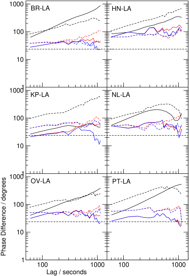
?figurename? 6.8: Structure functions from 25 min of observation of NGC 4261 at 43 GHz (the structure functions have been cut off after 1150 s due to a lack of points at longer lags). Solid black lines show raw data observed at night with delay calibration only, solid red lines show the same data calibrated with scaled-up phase solutions from fringe-fitting at 15 GHz, and solid blue lines show the same data without the residual phase rate. Dashed lines show the same stages of calibration, respectively, but from a scan observed during the late evening, where ionospheric effects increased the phase noise. The horizontal dashed black lines indicate the theoretical phase noise. The median residual phase noise of calibrated data, with residual phase rates, is $33^{\circ}$ at night and $50^{\circ}$ during sunset, and without residual phase rates is $31^{\circ}$ at night and $44^{\circ}$ during sunset.

?figurename? 6.9: The effect of ionospheric corrections. NGC 4261 calibrated 43 GHz visibility phases on baselines to Los Alamos as in Fig. 6.6 (lower panel), but no ionospheric correction has been applied. The residual phase rates are much higher.

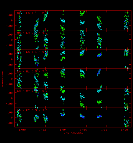
?figurename? 6.10: The effect of using a model in self-calibration. NGC 4261 calibrated 43 GHz visibility phases on baselines to Los Alamos. Calibration has been done with scaled-up phase solutions from fringe-fitting at 15 GHz using a point source model (light blue) and a clean component model (green), showing the effect of source structure at 15 GHz in the calibration at 43 GHz.

           

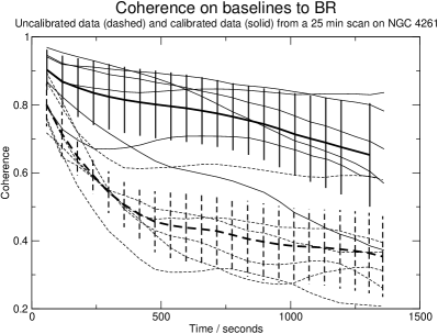
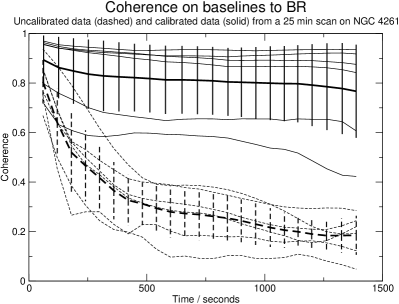
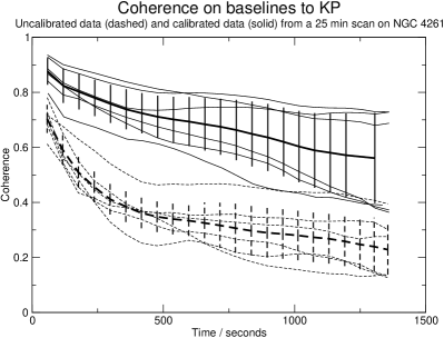
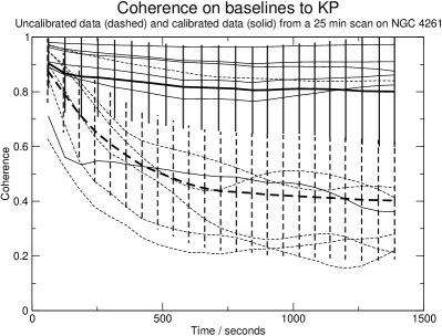
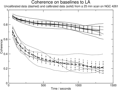
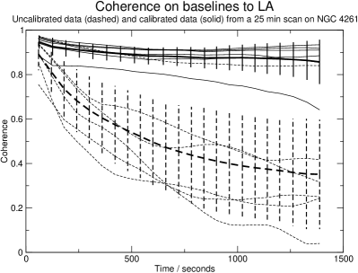
?figurename? 6.11: Coherence improvement at 43 GHz. NGC 4261 was observed in the early evening (centred on 01:06 UT, left column) and at night (centred on 03:40 UT, right column) at 43 GHz with interleaved 15 GHz observations for calibration. 43 GHz data with (solid lines) and without (dashed lines) phase-calibration from 15 GHz have been averaged in frequency and in time over each 43 GHz half-cycle. The normalized vector sum has been computed on all baselines to a given station over progressively larger time intervals and assuming unit amplitude. Bold lines show the average over all baselines.

?figurename? 6.12: Naturally weighted, full-resolution image of NGC 4261 at 43 GHz, calibrated with scaled-up phase solutions from 15 GHz. FRING has been used to solve for one residual phase and rate solution per 25 min scan before exporting the data to Difmap. No further self-calibration has been applied. The image noise is 4.4 mJy beam^-1 and the dynamic range is 18:1.

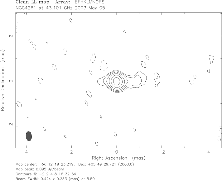
?figurename? 6.13: Data and imaging parameters as in Fig. 6.12, but several cycles of phase self-calibration with a solution interval of 30 s and one cycle of amplitude self-calibration with a solution interval of 12 h have been applied. The image noise is 0.78 mJy beam^-1 and the dynamic range is 122:1.

?figurename? 6.14: 86 GHz visibility phases. Top: NGC 4261 raw 86 GHz visibility phases on baselines among Fort Davis, Kitt Peak, Los Alamos, Owens Valley and Pie Town with only delay calibration applied. Bottom: 86 GHz visibility phases on baselines among Fort Davis, Kitt Peak, Los Alamos, Owens Valley and Pie Town. Calibration has been done with scaled-up phase solutions from fringe-fitting at 15 GHz using a clean component model. Good detections were made during almost every 25 min scan observed at night between 2:00 h UT and 7:00 h UT, when the ionosphere was stable.

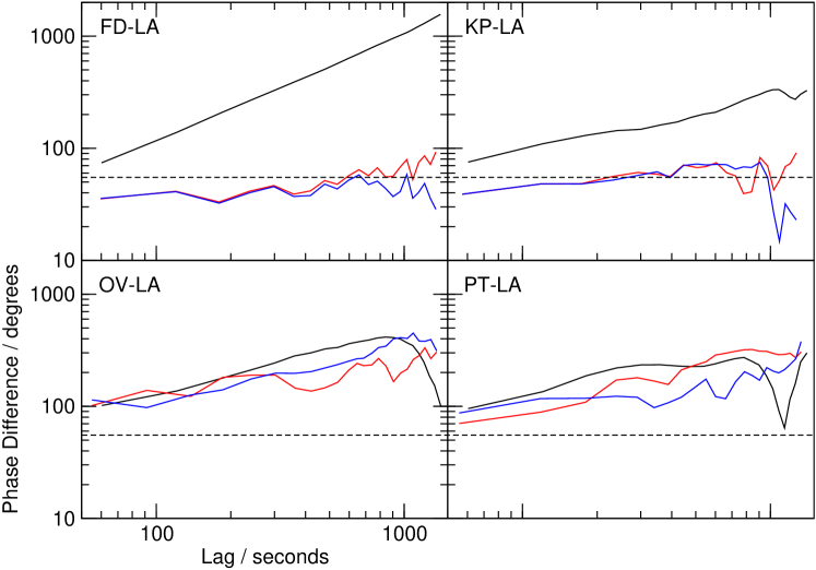
?figurename? 6.15: Structure functions of a 25 min scan at 86 GHz. Colours show the same stages of calibration as is Fig. 6.8.

       

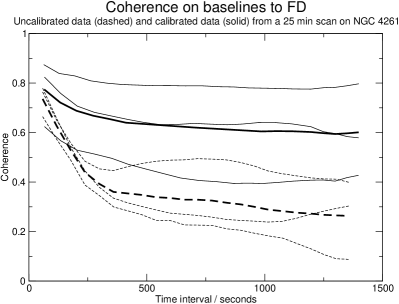
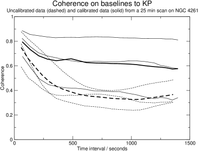
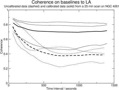
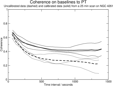
?figurename? 6.16: The coherence improvement at 86 GHz with fast frequency switching on some of the baselines shown in Fig. 6.14. Errors have not been computed due to the reduced number of data points.

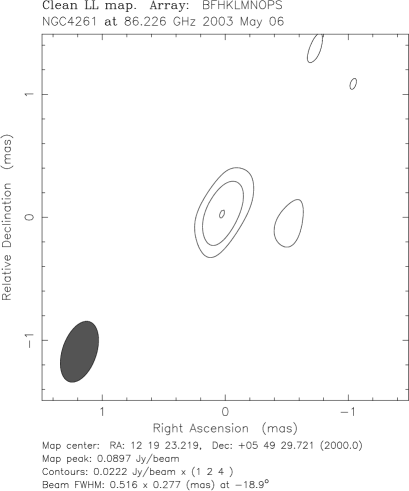
?figurename? 6.17: 86 GHz images of NGC 4261. Top: Naturally weighted, full-resolution image of NGC 4261 at 86 GHz, calibrated with scaled-up phase solutions from 15 GHz. FRING has been used to solve for one residual phase and rate solution per 25 min scan before exporting the data to Difmap. No further self-calibration has been applied. The image noise is 8.4 mJy beam^-1 and the dynamic range is 7:1. Bottom: Data and imaging parameters as above, but several cycles of phase self-calibration have been applied. The image noise is 7.4 mJy beam^-1 and the dynamic range is 12:1.

?chaptername? 7 Conclusions

In an attempt to measure the magnetic field strength in the sub-pc scale environment of AGN through Faraday rotation, we have used the VLBA at 15.4 GHz to look for polarized emission in NGC 3079, NGC 1052, NGC 4261, Hydra A, Centaurus A and Cygnus A. We selected these nearby ($D<200\,{\rm Mpc}$) objects for high linear resolution and good evidence for free-free absorption in a foreground medium. If the medium is interspersed with a magnetic field, Faraday rotation is expected to occur. Surprisingly, we did not detect any polarized emission in five out of six sources, and we found one source (Cygnus A) to be polarized at a level of only $(0.44\pm 0.3)\,\%$. The results for one source (Centaurus A) were inconclusive due to poor $(u,v)$ coverage. The non-detection of polarized emission is not unexpected in regions where a dense free-free absorber is seen, but is unexpected for regions that apparently are unabsorbed. We have supplemented our observations of NGC 3079 with multi-epoch, multi-frequency VLBI observations to study spectral properties and proper motions. From our study, we draw the following conclusions.

1. The non-detection of polarized emission is significantly different from VLBI surveys targeted at highly beamed quasars. We find that our selection criteria biased the sample towards unbeamed, double-sided radio jets in which circumnuclear absorbers are seen edge-on.

2. We expect that the radio emission from the sources is synchrotron emission which is intrinsically polarized, and conclude that the radiation is depolarized in a foreground screen. The rotation measure in the screen must be variable on scales much smaller than the synthesized beam size so that differential Faraday rotation causes a net decrease of polarized emission when averaged across the beam area. In our sources, such screens are detected through their free-free absorption only in very small regions across parts of the radio jets where they are interpreted as free-free absorption in circumnuclear tori, but their opacity rapidly decreases away from that region and they are not detected along the jets. This imposes constraints on the physical parameters in the foreground screen. The screen must be dense enough to depolarize at the relatively high frequency of 15.4 GHz and at the same time, must be transparent to radio emission along most of the jet. We find that the electron density in the screen must be of the order of $25\,{\rm cm^{-3}}$ for magnetic fields of the order of 0.1 mG and for path lengths of a few parsecs.

3. Considering possible absorbers in front of the jets in which the Faraday depolarization occurs, we present a model in which ionized material is accreted in a spherical flow from scales of $>10\,{\rm pc}$ to sub-pc scales (Bondi accretion). Assuming equipartition magnetic fields, the model predicts the necessary Faraday rotation and, at the same time, is transparent to radio emission at 15.4 GHz. The accretion rates are probably signifcant lower in the Seyferts NGC 3079 and NGC 1052 than in the other four objects, and the rotation measures predicted by the model are too low. However, we cannot rule out that the depolarization in these two objects is due to a combination of the ionized fraction of the interstellar gas, H II regions and NLR clouds.

4. Our observations of NGC 3079 have yielded the following additional results. In two radio components, $A$ and $E$, we find good evidence for a foreground free-free absorber, with column densities of the order of $10^{22}\,{\rm cm^{-2}}$. The intrinsic (unabsorbed) spectrum of $E$ is extremely steep, with $\alpha=-4.1$, the best explanation of which is by a non-power-law distribution of electron energies. The spatial distribution of peak frequencies found in four components in NGC 3079 is suggestive of a foreground absorber with a density gradient.

We find proper motions of the order of $0.1\,c$ among the three strongest components, $A$, $B$ and $E$. The lack of absolute positions for all but the last epoch did not allow us to define a kinematic centre in NGC 3079, but we prefer a scenario in which either $B$ is stationary (possibly equvalent to the case in which the kinematic centre is not coincident with any of the components) or the components move on helical trajectories. If $B$ is stationary, component $E$ is moving towards the AGN, which is unexpected.

In a statistical analysis of VLBI observations of Seyfert galaxies, we find that the spectral and structural properties of NGC 3079 are not uncommon, though the spectra are at the positive end of the distribution.

5. For higher resolution observations of nearby and hence mostly weak AGN, we have developed the phase-referencing strategy of fast frequency switching, in which the source is observed continuously while rapidly switching between the target frequency and a lower reference frequency. Phase solutions from self-calibration at the low frequency are multiplied by the frequency ratio and are used to calibrate the high-frequency visibilities. We describe the strategy and results of an observation of NGC 4261. We found that short-term phase fluctuations at 43 GHz and 86 GHz can be calibrated with residual rms phase errors of $33^{\circ}$ and $70^{\circ}$, respectively using interleaved 15 GHz scans. Ionospheric phase fluctuations on timescales of minutes to hours caused residual phase drifts of up to a turn of phase and did not allow us to fully calibrate the data without self-calibration. We present the first detection of NGC 4261 at 86 GHz which was not possible with conventional VLBI because it is weak. To our knowledge, this is so far the weakest source detected with VLBI at that frequency.

?chaptername? 8 Danksagung

Die Danksagung wird oft als das schwierigste Kapitel einer Doktorarbeit bezeichnet, und angesichts der grossen Anzahl von Menschen, denen ich zu Dank verpflichtet bin, beinhaltet diese Aussage wohl einen Funken Wahrheit.

Zunächst möchte ich meinen Referenten Prof. Ulrich Klein und Priv. Doz. Walter Huchtmeier danken, die die Arbeit des Nachsehens auf sich genommen haben. Sie haben mir darüber hinaus in zahlreichen Gesprächen hilfreich zur Seite gestanden und wichtige Impulse gegeben, die meine Arbeit in die vorliegende Form gebracht haben.

Den Direktoren des MPI möchte ich für die Möglichkeiten danken, die mir durch meine Anstellung am Institut zuteil wurden. Insbesondere die zahlreichen Dienstreisen und Konferenzen haben meinen Horizont beträchtlich erweitert. Dr. Anton Zensus bin ich darüber hinaus für zahlreiche Gespräche dankbar, die den Fortgang meiner Arbeit und die Planungen für die Zeit danach betrafen. Auch Dr. Arno Witzel hat mir hier oft weiter geholfen.

Einer der schönsten Aspekte meiner Zeit am MPI war sicherlich das Arbeiten in einer so freundlichen Gruppe mit so vielen Menschen, die ihr Wissen bereitwillig weiter geben, und allen gebührt mein aufrichtiger Dank. Insbesondere danken möchte ich Dr. Andrei Lobanov und Dr. Eduardo Ros für zahlreiche Diskussionen zur AGN-Physik und Astrometrie; Dr. Richard Porcas für geduldige Erklärungen und interessante Diskussionen zu den zahlreichen Fallstricken in VLBI und für das Nachsehen von Teilen dieser Arbeit; Dr. Thomas Krichbaum für seine Unterstützung meiner Projekte und Ratschläge zu Proposals sowie ebenfalls für Korrekturen; Dr. Thomas Beckert für zahlreiche Erläuterungen theoretischer Zusammenhänge; Dr. Walter Alef für Erklärungen zum Korrelator und seine nimmermüde Hilfsbereitschaft in Computerangelegenheiten; Dr. Alex Kraus für seine Hilfe in Effelsberg und zur Datenreduktion und Prof. Heino Falcke für seine Beiträge und Ideen zu meiner Arbeit. Macht weiter so!

Nicht zu unterschätzen ist auch der Beitrag der Studenten zu diesem Arbeitsklima, und dafür bin ich allen dankbar. Hervorheben möchte ich Tim Huege und Elmar Körding, die mir in Dingen der Mathematik hilfreich zur Seite standen (außerdem werde ich den täglichen 12 Uhr-Anruf vermissen). Matthias Kadler, Violetta Impellizzeri und Uwe Bach haben nicht nur eine sehr angenehme Büroatmosphäre geschaffen, sondern waren immer zu Diskussionen bereit, um die täglichen Probleme zu lösen. Mit Uwe Bach verbindet mich nun auch ein nahezu neunjähriges Studium, und ohne ihn wären so einige Hürden höher und viele Probleme schwieriger gewesen, und dafür bin ich sehr dankbar. Außerdem gebührt allen anderen Mitarbeitern des MPI, von der Materialstelle über die Verwaltung bis zur Rechnerabteilung, ein recht herzliches Dankeschön.

Von außerhalb des MPI habe ich Dr. Andrew Wilson für seine ausführlichen Bemerkungen zur Statistik der Seyfert-Galaxien und Dr. Denise Gabuzda für ihre Hilfe bei der Polarimtrie zu danken. Dr. Craig Walker hatte einen erheblichen Anteil an der Entwicklung des Fast Frequency Switchings, und die Zeit in Socorro bleibt unvergeßlich.

Für Dr. Alan Roy fehlen mir die Worte und es wäre sinnlos, das durch unzureichende Umschreibungen zu verdecken. Vielen, vielen Dank, Alan.

Meinen Eltern danke ich für ihre Unterstützung, ihre Liebe und ihren Optimismus, und Angelika für alles, was uns verbindet.