Microlensing by the Halo MACHOs with Spatially Varying Mass Function

Abstract

The main aim of microlensing experiments is to evaluate the mean mass of massive compact halo objects (MACHOs) and the mass fraction of the Galactic halo made by this type of dark matter. Statistical analysis shows that by considering a Dirac-Delta mass function (MF) for the MACHOs, their mean mass is about that of a white dwarf star. This result is, however, in discrepancy with other observations such as those of non-observed expected white dwarfs in the Galactic halo which give rise to metal abundance, polluting the interstellar medium by their evolution. Here we use the hypothesis of the spatially varying MF of MACHOs, proposed by Kerins and Evans to interpret microlensing events. In this model, massive lenses with a lower population contribute to the microlensing events more frequently than do dominant brown dwarfs. This effect causes the mean mass of the observed lenses to be larger than the mean mass of all the lenses. A likelihood analysis is performed to find the best parameters of the spatially varying MF that are compatible with the duration distribution of Large Magellanic Cloud microlensing candidates of the MACHO experiment.

1 Introduction

The rotation curves of spiral galaxies (including Milky Way) show that this type of galaxies have dark halo structure Borriello & Salucci (2001). One of the candidates for the dark matter in the Galactic halo may be massive compact halo objects (MACHOs). Paczyński (1986) proposed a gravitational microlensing technique as an indirect way of detecting MACHOs. Since his proposal, many groups began monitoring millions of stars of the Milky Way in the directions of the spiral arms, the Galactic bulge and the Large and Small Magellanic Clouds (LMC & SMC) and detected hundreds of microlensing candidates Ansari (2004); Derue et al. (2001); Sumi et al. (2003); Afonso et al. (2003). Looking in the direction of the LMC and SMC (which are the most important for estimating Galactic halo MAHCOs), Expérience de Recherche d’Objets Sombres (EROS) and MACHO observers found only a dozen of microlensing candidates Lasseree et al. (2000); Alcock et al. (2000). The interpretation of LMC and SMC events is based on the statistical analysis of the distribution of the duration of the events. The result of this analysis attribute a mean mass to MACHOs and their mass contribution in the Galactic halo. With the standard halo model, the mean mass of lenses is evaluated to be about half of that of the solar mass with a 20 per cent contribution in the Galactic halo mass.
The results obtained by the analysis of LMC microlensing events, however, do not agree with other observations Gates & Gyuk (2001). Studying the kinematics of white dwarfs that have been discovered Oppenheimer et al. (2001) has shown that halo white dwarfs corresponds to $1-2$ per cent of the halo mass. Recent re-analysis of the same data Spagna et al. (2004); Torres et al. (2002) shows that this fraction is an order of magnitude smaller than the value derived in Oppenheimer et al. (2001). On the other hand, if there were as many white dwarfs in the halo as suggested by the microlensing experiments, they would increase the abundance of heavy metals via the evolution of white dwarfs and Type I Supernova explosions Canal et al. (1997). The other problem is that for the mass of the MACHOs to be in the range proposed by microlensing observations, the initial mass function (IMF) of MACHO progenitors of the Galactic halo should be different from those of the disc Adams & Laughlin (1996); Chabrier et al. (1996), otherwise we should observe at the tail of mass function (MF) a large number of luminous stars and heavy star explosions in the Galactic halos.
In this study we use the hypothesis of a spatially varying MF (instead of uniform Dirac-Delta MF for the halo MACHOs) to interpret the LMC microlensing candidates (Kerins & Evans 1998, hereafter KE). The physical motivation for the hypothesis of spatially varying MFs of MACHOs comes from baryonic cluster formation theories Ashman (1990); Carr (1994); De Paolis et al. (1995). These models predict the spatial variation of MF in the galactic halo in such a way that the the inner halo comprises partly visible stars, in association with the globular cluster population, while the outer halo comprises mostly low-mass stars and brown dwarfs.
We extend the work of KE by (i) using spatially varying MF model in the power-law halo model Alcock et al. (1996), including the contribution disc, spheroid and LMC for comparison with the latest (5 yr ) LMC microlensing data (Alcock et al. 2000); (ii) using a statistical approach applied by Green & Jedamzik (2002) and Rahvar (2004) to compare the distribution of the duration of the observed events with the galactic models; and (iii) performing a likelihood analysis to find the best parameters of the inhomogeneous MF model.
The advantage of using spatially varying MF models is that the active mean mass of lenses as the mean mass of observed lenses is always larger than mean mass of overall lenses. This effect is shown by a Monte-Carlo simulation, and taking it into account may resolve the problems with interpreting microlensing data.
This paper is organized as follows. In Section 2 we give a brief account of the hypothesis of spatially varying MFs and the galactic models used in our analysis. In Section 3 we perform a numerical simulation to generate the expected distribution of events, taking into account the observational efficiency of the MACHO experiment. In Section 4 we compare the theoretical distribution of the duration of the events with the observation. We also perform a likelihood analysis to find the best parameters of the MF for compatibility with the observed data. The results are discussed in Section 5.

2 Matter distribution in the Galactic Models

Spiral galaxies have three components: the halo, the disc and the bulge. We can combine these components to build various galactic models Alcock et al. (1996). In this section we give a brief account on the power-law halo and disc models which can contribute to the LMC microlensing events. In the second part we discuss about MFs of MACHOs and our physical motivation for considering spatially varying MFs.

	Model :	$S$	$A$	$B$	$C$	$D$	$E$	$F$	$G$
(1)	Description	Medium	Medium	Large	Small	E6	Maximal	Thick	Thick
(2)	$\beta$	–	0	-0.2	0.2	0	0	0	0
(3)	$q$	–	1	1	1	0.71	1	1	1
(4)	$v_{a}(km/s)$	–	200	200	180	200	90	150	180
(5)	$R_{c}(kpc)$	5	5	5	5	5	20	25	20
(6)	$R_{0}(kpc)$	8.5	8.5	8.5	8.5	8.5	7	7.9	7.9
(7)	$\Sigma_{0}(M_{\odot}/pc^{2})$	50	50	50	50	50	100	80	80
(8)	$R_{d}(kpc)$	3.5	3.5	3.5	3.5	3.5	3.5	3	3
(9)	$h(kpc)$	0.3	0.3	0.3	0.3	0.3	0.3	1	1
(10)	$\sigma_{v}(km/s)$	31	31	31	31	31	31	49	49

Table 1: The parameters of the eight Galactic models: First line is the description of the models in terms of the disk, second line the slope of rotation curve $(\beta=0$ flat, $\beta<0$ rising and $\beta>0$ falling), third line the halo flattening ($q=1$ represent spherical), fourth line $(v_{a})$ the normalization velocity, fifth line $R_{c}$ halo core, sixth line distance of the sun from the center of galaxy, seventh line the local column density of the disk ($\Sigma_{0}=50$ for canonical disk, $\Sigma_{0}=80$ for maximal thin disk and $\Sigma_{0}=40$ for thick disk), eighth line disk scalelength, the ninth line disk scalehight and tenth line is the adopted one-dimensional velocity dispersion of disk, perpendicular to our line of sight.

2.1 Power-law halo mode

A large set of axisymmetric galactic halo models are the ”power law ” models with a matter density distribution given by Evans (1994) :

$$\rho(R,z) = \frac{{V_{a}}^{2}{R_{c}}^{\beta}}{4\pi Gq^{2}}$$ (1)

$$\times \frac{{R_{c}}^{2}(1+2q^{2})+R^{2}(1-\beta q^{2})+z^{2}[2-(1+\beta)/q^{2}]}{({R_{c}}^{2}+R^{2}+z^{2}/q^{2})^{(\beta+4)/2}},$$

where $R$ and $z$ are the coordinates in the cylindrical system, $R_{c}$ is the core radius and $q$ is the flattening parameter which is the axial ratio of the concentric equipotentials, the parameter $\beta$ determines whether the rotational curve asymptotically rises, falls or is flat and the parameter $V_{a}$ determines the overall depth of the potential well and hence gives the typical velocities of objects in the halo. The dispersion velocity of particles in the halo can be obtained by averaging the square of the velocity over the phase space.
Apart from the Galactic halo, there are other components of the Milky Way such as the Galactic disc, spheroid and LMC disc that can contribute to the LMC microlensing events. The matter distribution of the disc is described by double exponentials Binney & Tremaine (1987) and the MF of this structure is taken according to the Hubbel Space Telescope (HST) observations (Gould., Bahcall & Flynn 1997). The second component of the Milky Way which may also contribute to the microlensing events is the Milky Way Spheroid. The spheroid density is given by $\rho_{spher}=1.18\times 10^{-4}(r/R_{0})^{-3.5}M_{\odot}pc^{-3}$, where $R_{0}$ is the distance of the Sun from the center of Galaxy (Guidice., Mollerach & Roulet 1994; Alcock et al 1996). We take the dispersion velocity for this structure to be $\sigma_{v}=120km/s$. The matter density of LMC disc as the third structure that can contribute to the microlensing events is also described as a double exponential with the parameters $R_{d}=1.57kpc$, $h=0.3kpc$ and $\sigma=25km/s$, where $R_{d}$ is the disc scalelength, $h$ is the disc scalehight and $\sigma$ is the dispersion velocity Gyuk et al. (2000).
The combination of galactic substructures as galactic models denoted by $S,A,B,C,D,E,F$ and $G$. The parameters of these models are given in Table. 1.

2.2 Spatially varying mass function

The tradition in the interpretation of gravitational microlensing data is to use the Dirac-Delta function as the simplest MF of Galactic halo MACHOs. Colour-magnitude diagram studies of the population of stars in the Galactic disc, bulge and other galaxies show that MF behaves like a power law function, where the mean mass of the stars depends on the density of interstellar medium where the stars have been formed. Following this argument, the MF of MACHOs in the Galactic halo may also follow a power-law function. Fall & Rees (1985) proposed a cooling mechanism for the globular cluster formation and on the same basis, the hydrogen clouds cooling mechanism can produce a cluster of brown dwarfs (Ashman 1990). The dependence of the mass of stars on the density of the star formation medium may causes the heavy MACHOs produced in the dense inner regions and the light ones at the diluted areas of the halo boarder.
Here in our study we use $MF(r)=\delta[M-M(r)]$ as the simplest spatially varying MF, proposed by KE. The mass scale $M(r)$ in this model decreases monotonically as $M_{U}(\frac{M_{L}}{M_{U}})^{r/R_{halo}}$, where $r$ is the distance from the center of the Galaxy, $M_{L}$ and $M_{U}$ are the mass scales representing the lower and upper limits of the mass function and $R_{halo}$ is the size of Galactic halo contains MACHOs. Considering the cold dark matter component for the the halo, the size of the Galactic halo may be larger than $R_{halo}$.

3 Microlensing Events in the Spatially Varying MF

In this section our aim is to generate microlensing events in the spatially varying MF and compare them with the observed data. The overall rate of microlensing events owing to the contribution of the halo, disk, spheroid and LMC itself is given by

$$\frac{d\Gamma}{dt}=f\frac{d\Gamma}{dt}(halo)+\frac{d\Gamma}{dt}(disk)+\frac{d\Gamma}{dt}(spheroid)+\frac{d\Gamma}{dt}(LMC),$$ (2)

where, $f$ is the fraction of the halo made by the MACHOs. The parameter $f$ can be obtained by comparing the observed optical depth with that of the expected value from the galactic models Alcock et al. (1995). The observed optical depth is given by $\tau_{obs}=\frac{\pi}{4E}\Sigma t_{i}$ , for 13 microlensing candidates of the MACHO experiment (see Table 3) where $E=6.12\times 10^{7}$ objects-years exposure time, $\tau_{obs}=4.43\times 10^{-8}$ Alcock et al. (2000). The observed optical depth is sensitive to our estimation of the duration of the events. On the other hand, the theoretical optical depth is given by

$$\tau_{expected}=\frac{\pi}{4}\int{\frac{d\Gamma}{dt}\epsilon(t)tdt},$$ (3)

where $\epsilon(t)$ is the observational efficiency. Table 2 shows the results of comparison between the theoretical and observed optical depths. We use the evaluated value of $f$ in each model to obtain the distribution of the duration of events. Fig. 1 compares the normalized distributions of the duration of events for uniform and spatially varying MFs in eight galactic models.
The advantage of using a spatially varying MF is that heavy MACHOs in the Galactic halo contribute to gravitational microlensing events more frequently than do dominant-light MACHOs. This effect can be shown by a Monte-Carlo simulation. Before explaining the simulation we introduce two parameters of the passive and active mean masses of lenses. The passive mean mass is defined as the mean mass of the overall lenses of the Galactic halo. This mass is independent of the gravitational microlensing observation and can be obtained directly by averaging over the masses of MACHOs

$$<M>_{passive} = \frac{\int\phi[M,x]M(x)d^{3}xdM}{\int\phi[M,x]d^{3}xdM},$$ (4)

$$= \frac{\int\rho(x)d^{3}x}{\int\frac{\rho(x)}{M(x)}d^{3}x},$$

the second equation is obtained by substituting the spatially varying MF model.
In contrast to the passive mean mass, we define the active mean mass of lenses as the mean mass of observed microlensing candidates. It is clear that in the case of a uniform Dirac-Delta MF, these two masses are equal, but in the spatially varying MF, the active mean mass of lenses is always larger than the passive one.
The algorithm of our simulation for evaluating the active mean mass of lenses is (i) selecting the position of lenses according to the position distribution function of MACHOs along our line of sight; (ii) calculating duration of the events $(t_{e})$ and comparing them with the observational efficiency of MACHO experiment and (iii) calculating the mean mass of selected evens. To select the location of a lens, we imagine that we make observations for a given interval of $T_{obs}$. The probability that a MACHO is located at a distance $x=\frac{D_{l}}{D_{s}}$ from the observer playing the role of a lens, thereby magnifying one of the background stars of the LMC, is

$$\frac{d\Gamma}{dx}=4\sqrt{\frac{GD_{s}}{M(x)c^{2}}x(1-x)}v_{t}(x)\rho(x),$$ (5)

where $M(x)$ is the mass of the MACHO and can be substituted by the spatially varying MF model and $v_{t}(x)$ is the transverse velocity of the lens with respect to our line of sight. The duration of the events (after picking up the location of lenses) is obtained by $t_{e}=\frac{2R_{E}(x)}{v_{t}(x)}$. Each time at the the Monte-Carlo simulation loop, by comparing the duration of the event with the observational efficiency of the MACHO experiment, the event is selected or rejected. The mass of selected events are used to calculate the mean mass of observed MACHOs. Table 2 shows the results of our simulation, the passive $<M_{ml}>$ and active $<\widetilde{M}_{ml}>$ mean mass of lenses for different galactic models. As we expected, in all the galactic models the active mean mass is always larger than the passive one. This means that in spite of the light abundant brown dwarfs in the Galactic halo, lenses with the larger masses produce most microlensing events.

4 Comparison of the microlensing candidates with the galactic models

In this section our aim is to compare the expected events from the spatially varying MF with the microlensing candidates. The next step is to find the best parameters for the spatially varying MF model which are compatible with the data. Two statistical parameters, the width of the distribution of the duration of the events and its mean value are used in our comparison. These parameters are defined as follows Green & Jedamzik (2002); Rahvar (2004):

Figure 1: The normalized distribution of events duration in the galactic models of $Standard,A,B,C,D,E,F$ and $G$, multiplied to the observational efficiency of MACHO experiment. The solid and dashed lines represent the distributions of events in the uniform and spatially varying Dirac-Delta MFs. The dash-dotted line is resulted from the likelihood analysis for the best parameters of KE model to be compatible with the observed data. The duration distributions indicated by solid and dashed-dotted are similar while the dashed-line which represents the KE model is different than them.

Figure 2: The expected distributions of the mean (left column) and the width (right column) of the duration of events are shown for the $Standard$, $A$, $B$ and $C$ Galactic models. The cross indicates the values of $<t_{e}>$ and $\Delta t_{e}$ from the 13 microlensing candidates of MACHO experiment. These distributions are shown for three categories of uniform Dirac Delta MF (solid line), KE spatially varying MF (dashed line) and KE model with the parameters derived from the likelihood analysis (dash-dotted lines). Most of the galactic models in the spatially varying MF with the optimized parameters are compatible with the observed data.

Figure 3: The expected distributions of the mean (left column) and the width (right column) of the duration of events are shown for the $D$, $E$, $F$ and $G$ Galactic models. The cross indicates the values of $<t_{e}>$ and $\Delta t_{e}$ from the 13 microlensing candidates of MACHO experiment These distributions are shown for three categories of uniform Dirac Delta MF (solid line), KE spatially varying MF (dashed line) and KE model with the parameters derived from the likelihood analysis (dash-dotted lines). Most of the galactic model in the spatially varying MF with the optimized parameters, except model E are compatible with the observed data.

$$\Delta t_{e} = Max(t_{e})-Min(t_{e}),$$ (6)

$$<t_{e}> = 1/N\Sigma t_{e}.$$ (7)

$\Delta t_{e}$ and $<t_{e}>$ for the LMC candidates are $188$ and $97$ d, respectively (see Table 3). We perform a Monte Carlo simulation to generate the mentioned statistical parameters from the theoretical distribution of $t_{e}$ for comparison with the observations. In this simulation we make an ensemble of 13 microlensing events where those events are picked up from the theoretical distribution of the duration and in each set of events, the mean and the width of the duration of the events are calculated. The mean of and the width from each set is used to generate the distributions.

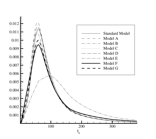
Figure 4: The duration distribution of events in eight galactic models with the spatially varying MF, where the MF parameters are optimized to be compatible with the data by the likelihood analysis. The expected distribution of events can be obtained by multiplying the duration distribution to the observational efficiency of microlensing experiment.

$Events(1)$	$Model(2)$	$MF(3)$	$halosize(kpc)(4)$	$M_{L}(5)$	$M_{U}(6)$	$<M_{ml}>(7)$	$<\widetilde{M}_{ml}>(8)$	$f_{ML}(9)$
13	S	$U$	–	–	–	0.54	0.54	0.20
13	S	$KE$	100	$10^{-3}$	3	0.05	0.44	0.16
13	S	$LA$	126	$10^{-3}$	1	0.16	0.26	0.2
6	A	$U$	–	–	–	0.32	0.32	0.41
13	A	$KE$	100	$10^{-3}$	3	0.19	1.05	0.13
13	A	$LA$	177	$10^{-3}$	0.5	0.16	0.31	0.14
13	B	$U$	–	–	–	0.66	0.66	0.12
13	B	$KE$	100	$10^{-3}$	3	0.17	0.97	0.1
13	B	$LA$	163	$10^{-3}$	0.9	0.22	0.5	0.1
6	C	$U$	–	–	–	0.21	0.21	0.61
13	C	$KE$	50	$10^{-3}$	10	0.008	1.1	0.27
13	C	$LA$	85	$10^{-3}$	0.5	0.04	0.21	0.25
6	D	$U$	–	–	–	0.31	0.31	0.37
13	D	$KE$	100	$10^{-3}$	3	0.2	1.21	0.13
13	D	$LA$	103	$10^{-3}$	0.4	0.06	0.2	0.12
6	E	$U$	–	–	–	0.04	0.04	2.8
13	E	$KE$	50	$10^{-3}$	10	0.007	0.31	1.05
13	E	$LA$	87	$10^{-3}$	0.5	0.04	0.15	0.8
13	F	$U$	–	–	–	0.19	0.19	0.39
13	F	$KE$	200	$10^{-3}$	2	0.54	0.99	0.33
13	F	$LA$	96	$10^{-3}$	0.4	0.04	0.13	0.3
6	G	$U$	–	–	–	0.21	0.21	0.71
13	G	$KE$	200	$10^{-3}$	2	0.56	1.05	0.18
13	G	$LA$	110	$10^{-3}$	0.3	0.05	0.13	0.18

Table 2: The first column gives the number of microlensing events that have been observed during 2 or 5.7 yrs monitoring of LMC stars by the MACHO group. The second column indicates the name of eight galactic models as described in Table 1. The third column specifies the MF in each model where $U$ indicates the uniform Dirac Delta MF which has been obtained by MACHO group, $KE$ indicates the MF proposed by Kerins and Evans (1998) and $LA$ indicates the MF which has been obtained by the likelihood analysis. The fourth column shows the size of halo that MACHOs are extended. The fifth column is the lower limit for the mass of MACHOs that are located at the edge of halo and the sixth column is the upper limit for the mass of MACHOs that reside at the center of halo. The seventh column is the mean mass of the MACHOs in each model, so-call passive mean mass of the lenses and the eighth column is the active mean mass of the observed lenses by the experiment. The ninth column shows the halo fraction made by MACHOs in each model.

$Event:$	1	4	5	6	7	8	13	14	15	18	21	23	25
$t_{E}$ (days)	34.5	83.3	109.8	92	112.6	66.4	222.7	106.5	41.9	75.8	141.5	88.9	85.3

Table 3: Microlensing candidates observed by the MACHO experiment during 5.7 yrs of observing 11.9 million LMC stars (Alcock et al. 2000). First row gives the name of the event according to numbering used by the MACHO group and second row shows the duration of event.

With this procedure we obtain the distributions of $\Delta t_{e}$ and $<t_{e}>$ for three categories of (i) Dirac-Delta MF; (ii) a spatially varying MF; and (iii) a spatially varying MF with the optimized parameters compatible with the data, resulting from the likelihood analysis. Figs. 2 and 3 compare the distributions of the observed $\Delta t_{e}$ and $<t_{e}>$ with three MF models used in eight power-law galactic models. Comparing the observed value, indicated by cross in Figs 2 and 3, with the theoretical distributions of $<t_{e}>$ and $\Delta t_{e}$, shows that for Dirac-Delta MF, some of the galactic models such as A, C and E are in agreement with the observations while for the KE model non of them are compatible with the data.
To find the spatially varying MF model that is compatible with the observations, we perform a likelihood analysis to obtain the best upper limit of the MACHO mass and the size of the halo in the KE model. The results of analysis in the power-law galactic models are shown in Table 2 with the corresponding distribution of the duration of events in Fig. 1. Figs. 2 and 3 show that the standard model and models A, B, C and D using this MF are in good agreement with the data.
In addition to the hypothesis of a spatially varying MF, there are other hypothesis, such as self-lensing, that need to be confirmed using sufficient statistics of microlensing events. Recent microlensing surveys such as Optical Gravitational Lensing Experiment (OGLE) and SuperMACHO are monitoring LMC stars and will provide more microlensing candidates over the coming years. To use the results of our analysis in the mentioned experiments, we obtained the theoretical distribution of events in each model without applying any observational efficiency (Fig. 4). The expected distribution of events in each experiment can be obtained by multiplying the observational efficiencies to these theoretical models.
It is worth to mention that our statistical analysis is sensitive to our estimation of the duration of the microlensing candidates. The correction with the blending effect can alter our result. The blending effect makes a source star to be brighter than its actual brightness, and the lensing duration appears shorter. The duration of a microlensing event can be determined from a light curve fit in which the brightness of the source star is included as a fitting parameter. The main problem with this standard method is the degeneracy caused by the fitting. High-resolution images by the HST have been used to resolve blending by random field stars in eight LMC microlensing events Alcock et al. (2001). The MACHO group also used another procedure where each event is fitted with a light curve that assumes no blending and then a correction is applied to the time-scale to account for the fact that blending tends to make the time scales appear shorter. This correction was determined from the efficiency of a Monte Carlo simulation, and it is a function of the time-scale of the measured event. The procedure is designed to give the correct average event time-scale, but it does not preserve the width of the time-scale distribution Bennet (2004). Green & Jedamzik (2002) and Rahvar (2004) showed that the width of duration of events derived from this method is narrower than the theoretical expectations.

5 Conclusion

In this work we extended the hypothesis of a spatially varying MF proposed by KE as a possible solution resolving discrepancies between microlensing results and other observations. The main point of this is to investigate the contradiction where microlensing experiments predict large numbers of white dwarfs which have not been observed.
The advantage of using a spatially varying MF is that we can modify our interpretation of microlensing data. We showed that in this model, in contrast to the Dirac-Delta MF, massive MACHOs contribute in the microlensing events more frequently than the low-mass ones do. To quantify our argument we defined two mass scales, the active mean mass of MACHOs as the mean mass of lenses that can be observed by the gravitational microlensing experiment and the passive mean mass of MACHOs as the overall mean mass of them. We showed that the active mean mass of MACHOs is always larger than the passive mean mass, except in the case of a uniform Dirac Delta MF where they are equal.
To test the compatibility of this model with the observed microlensing events, we compared the duration distribution of the events in this model with the LMC candidates of MACHO experiment. We used two statistical parameters - the mean and the width of the duration of events - to compare the observed data with the theoretical models. We showed that amongst power-low halo models some of them with a Dirac-Delta MF are compatible with the data, while in the case KE model, almost none of them are compatible with the data. The best parameters for the KE model were obtained with likelihood analysis. In the spatially varying MF using the new parameters, some Galactic models (such as standard model and models A, B, C and D) were compatible with the data. The hypothesis of a spatially varying MF of MACHOs may be tested by measuring the proper motions of white dwarfs in the Galactic halo Torres et al. (2002).

ACKNOWLEDGMENT
The author thanks David Bennett for his useful comments on blending correction of the duration of events and Sepehr Arbabi and Mohammad Nouri-Zonoz for reading the manuscript and giving useful comments.

References

- Adams & Laughlin (1996) Adams, F., Laughlin, G., 1996, ApJ, 468, 586
- Afonso et al. (2003) Afonso C. et al. (EROS), 2003, A&A, 404, 145
- Alcock et al. (1995) Alcock C. et al. (MACHO), 1995, ApJ, 449, 28
- Alcock et al. (1996) Alcock C. et al. (MACHO), 1996, ApJ, 461, 84
- Alcock et al. (2000) Alcock C. et al. (MACHO), 2000, ApJ, 542, 281
- Alcock et al. (2001) Alcock C. et al. (MACHO), 2001, ApJ, 552, 582
- Ansari (2004) Ansari R. (EROS), (astro-ph/0407583)
- Ashman (1990) Ashman K. 1990, MNRAS, 247, 662
- Bennet (2004) Bennett D. 2004, private communication
- Borriello & Salucci (2001) Borriello A., Salucci P., 2001, MNRAS, 323, 285
- Binney & Tremaine (1987) Binney S., Tremaine S., 1987, Galactic Dynamics, Princeton Univ. Press, Princeton, NJ
- Canal et al. (1997) Canal R., Isern J., Ruiz-Lapuente P., 1997, ApJ, 488, L35
- Carr (1994) Carr B. J. 1994, ARA&A, 32, 531
- Chabrier et al. (1996) Chabrier G., Segretain L., Mera D., 1996, ApJ, 468, L21
- De Paolis et al. (1995) De Paolis F., Ingrosso G., Jetzer P., & Roncadelli M. 1995, A&A, 295, 567
- Derue et al. (2001) Derue F. et al. (EROS), 2001, A&A, 373, 126
- Evans (1994) Evans N. W., 1994, MNRAS 267, 333
- Fall and Rees (1985) Fall S. M., Rees M., 1985, ApJ 298, 18
- Gates & Gyuk (2001) Gates I. E., Gyuk, G., 2001, ApJ, 547, 786
- Gould., Bahcall & Flynn (1997) Gould A., Bahcall J. N., Flynn C., 1997, ApJ, 482, 913
- Green & Jedamzik (2002) Green A. M., Jedamzik K., 2002, A&A 395, 31
- Guidice., Mollerach and Roulet (1994) Guidice G. F., Mollerach S., Roulet E., 1994, Phys. Rev. D, 50, 2406
- Gyuk et al. (2000) Gyuk G., Dalal N., Griest K., 2000, ApJ, 535, 90
- Kerins and Evans (1998) Kerins E., Evans N. W., 1998, ApJ, 503, 75
- Lasseree et al. (2000) Lasserre T. et al. (EROS), 2000, A&A, 355, L39.
- Oppenheimer et al. (2001) Oppenheimer B. R., Hambly N. C., Digby A. P., Hodgkin S, T., Saumon, D., 2001, Science, 292, 698
- Paczyński (1986) Paczyński B., 1986, ApJ, 304, 1
- Rahvar (2004) Rahvar S., 2004, MNRAS, 347, 213
- Spagna et al. (2004) Spagna A., Carollo, D., Lattanzi M. G., Bucciarelli, B., 2004, accpeted in A&A (astro-ph/0407557)
- Sumi et al. (2003) Sumi T. et al. (MAO), 2003, ApJ, 591, 204
- Torres et al. (2002) Torres, S., Garcia-Berro, E., Burkert, A., Isern, J, 2002, MNRAS, 336, 971.