Dust cloud formation in stellar environments

This paper reports on computational evidence for the formation of cloud-like dust structures around C-rich AGB stars. This spatio-temporal structure formation process is caused by a radiative/thermal instability of dust forming gases as identified by Woitke${\rm\hskip 3.44444ptet\hskip 3.01385ptal.\hskip 2.58334pt}$(2000). Our 2D (axisymmetric) models combine a time-dependent description of the dust formation process according to Gail${\rm\hskip 3.01385pt\&\hskip 3.01385pt}$Sedlmayr (1988) with detailed, frequency-dependent continuum radiative transfer by means of a Monte Carlo method (Niccolini${\rm\hskip 3.44444ptet\hskip 3.01385ptal.\hskip 2.58334pt}$2003) in an otherwise static medium ($\@vec{v}\!=\!0$). These models show that the formation of dust behind already condensed regions, which shield the stellar radiation field, is strongly favoured. In the shadow of these clouds, the temperature decreases by several hundred Kelvin which triggers the subsequent formation of dust and ensures its thermal stability. Considering an initially dust-free gas with small density inhomogeneities, we find that finger-like dust structures develop which are cooler than the surroundings and point towards the centre of the radiant emission, similar to the “cometary knots” observed in planetary nebulae and star formation regions. Compared to a spherical symmetric reference model, the clumpy dust distribution has little effect on the spectral energy distribution, but dominates the optical appearance in near IR monochromatic images.

1 Introduction

Dusty gases in space are often remarkably inhomogeneous. Numerous observations of various dust forming objects like the circumstellar environments of AGB and post-AGB stars, R Coronae Borealis stars, planetary nebulae, the ejecta of novae and supernovae, and even the hot winds generated by Wolf-Rayet stars, have shown that the dust forming medium usually possesses a clumpy internal structure. Reviews of such observations are given by Lopez (1999) and Woitke (2001).

The best-studied object in that respect is probably the infrared carbon star IRC+10216. Several infrared speckle observations of its innermost dust formation and wind acceleration zone show direct evidence for an irregular, possibly cloudy dust distribution around this late-type AGB star (Weigelt${\rm\hskip 3.44444ptet\hskip 3.01385ptal.\hskip 2.58334pt}$1998, Haniff${\rm\hskip 3.01385pt\&\hskip 3.01385pt}$Buscher 1998, Tuthill${\rm\hskip 3.44444ptet\hskip 3.01385ptal.\hskip 2.58334pt}$2000). Further evidence can be deduced from long-term $JHKL$ lightcurves. Concerning the carbon star II Lup, Feast${\rm\hskip 3.44444ptet\hskip 3.01385ptal.\hskip 2.58334pt}$(2003) argue for a restricted epoch of dust formation in a limited region along the line of sight, in order to explain a large-amplitude long-term decrease in $J$ whereas no corresponding increase in $K$ and $L$ was detected. Direct IR imaging and multi-wavelength IR lightcurves of the oxygen-rich red giant L$_2$ Pup point to similar wind asymmetries (Jura${\rm\hskip 3.44444ptet\hskip 3.01385ptal.\hskip 2.58334pt}$2002).

Additional hints to inhomogeneities in the environments of AGB stars are given by the patchy SiO maser spots observed in oxygen-rich Mira variables (e. g. TX Cam, Diamond${\rm\hskip 3.01385pt\&\hskip 3.01385pt}$Kemball 2003). On a larger scale, CO rotational emission lines provide evidence for local density enhancements in the winds of late-type stars, e. g. concerning the carbon star TX Psc (Heske${\rm\hskip 3.44444ptet\hskip 3.01385ptal.\hskip 2.58334pt}$1989) or in high-resolution observations of the detached shell of TT Cyg (Olofsson${\rm\hskip 3.44444ptet\hskip 3.01385ptal.\hskip 2.58334pt}$2000). Observations with higher spatial resolution, using instruments like the Vlti, Ngst or Alma, can be expected to reveal even more details in the near future.

Spherically symmetric dynamical models for AGB winds which include a time-dependent treatment of dust formation strongly suggest the formation of radial dust shells in more or less regular time intervals (e. g. Winters${\rm\hskip 3.44444ptet\hskip 3.01385ptal.\hskip 2.58334pt}$2000, Sandin${\rm\hskip 3.01385pt\&\hskip 3.01385pt}$Höfner 2003), even if the pulsation of the star is neglected (e.g. Fleischer${\rm\hskip 3.44444ptet\hskip 3.01385ptal.\hskip 2.58334pt}$1995). The question arises whether these dust shells remain spherical symmetric (as suggested by the 1D models), or whether they might break apart into clouds due to instabilities. We focus in this paper on the second possibility and study the two-dimensional time-dependent behaviour of the dust/gas mixture just during the formation of a new dust shell.

Clumpiness may also play a vital role for the photo-chemistry during the AGB$\,\to\,$PPN$\,\to\,$PN transition phase. Opaque clumps can suppress the photodissociation of certain molecules like Benzene, such that their existence has been proposed to be an indicator for inhomogeneities with large density contrasts (Redman${\rm\hskip 3.44444ptet\hskip 3.01385ptal.\hskip 2.58334pt}$2003).

Regarding other classes of objects, numerous opaque structures have been discovered in proto-planetary nebulae (e. g. the Helix nebula NGC 7293 and the Eskimo nebula NGC 2392) as well as in star formation regions (e. g. the Orion nebula). These neutral, dense, probably dusty regions, designated as “cometary knots”, “globules” or “proplyds”, are located at the head of radially aligned linear structures in these nebulae and are particularly well visible in high resolution images of emission line ratios like [OIII]/H$\alpha$ (O’Dell 2000).

The physical cause of the observed clumpiness is still puzzling. In Paper I of this series (Woitke${\rm\hskip 3.44444ptet\hskip 3.01385ptal.\hskip 2.58334pt}$2000), we have formulated the hypothesis that a radiative/thermal instability in dust forming gases can provoke a self-organisation of the matter, which is possibly involved in the formation of the observed structures. This instability is characterised by a physical control loop between the radiative transfer, which determines the temperature structure of the medium, and the dust formation, which determines its opacity (see Fig. 1 in Paper I).

This paper reports on computational evidence for this hypothesis. In Sect. 2, we outline the concept of our static model for the environment of a C-rich AGB star, which combines a time-dependent treatment of dust formation with two-dimensional radiative transfer. Section 3 shows and discusses the results, including the calculated optical appearance of a clumpy dust distribution in the spectral energy distribution and in monochromatic images. In Sect. 4, our conclusions are drawn.

2 The model

The spatio-temporal evolution of the dust component in the circumstellar environment of a C-rich AGB star is simulated by means of a 2D (axisymmetric) time-dependent model. Our aim is to investigate whether radiative/thermal instabilities can excite a spatio-temporal self-organisation of the dust forming medium. We do not intend to model any specific object. Instead, we are interested in what kind of spatial structures possibly develop and we want to identify which physical control mechanisms are responsible for the structure formation.

According to this purpose, the radiative, chemical and physical processes directly involved in the instability must be modelled as complete and precise as necessary. In our two-dimensional approach, a precise radiative transfer requires large computational efforts (see Sects. 2.5 and 2.6 for details) and with our current approach, we are already at the computational limit of todays super-computer facilities. Therefore, the remaining parts of the model must be kept comparably simple. For these reasons, we assume that the gas/dust mixture is static ($\@vec{v}\!=\!0$) and focus only on the time-dependent dust-chemistry and the radiative transfer. Another reason for this concept is that we want to study the pure effect of the instability, which might get entangled with other dynamical instabilities, if hydrodynamics was included. The question whether or not this model is realistic depends on the relation between the time-scales of the included processes (radiative transfer, chemistry and dust formation) and the hydrodynamical time-scale (see discussion in Paper I). If the formation of a new dust shell occurs on a much smaller time-scale than the hydrodynamical time-scale, the assumption of a quasi-static medium seems appropriate. Regarding the parameters of our standard model (see Fig. 2), in particular the stellar luminosity $L_{\star}\!=\!3000\,L_{\odot}$, it is not sure that enough radiation pressure can be provided to drive a dust-driven outflow, i. e. the hydrodynamical time-scale could be in fact quite large.

Our approach, at least, allows for a first exploration of the qualitative two-dimensional behaviour of the dust component in AGB star winds which, according to our knowledge, is the first multi-dimensional and time-dependent (though static) model for dust formation around a cool star which includes the important feedback of dust on the temperature structure of the medium via radiative transfer effects.

2.1 Gas density distribution

The time-dependent simulations of dust formation and radiative transfer are carried out for a restricted model volume, which covers the outer atmospheric layers of the star mainly responsible for the dust formation. Within this volume, the hydrogen nuclei particle density $n_{\langle{\rm H}\rangle}\,[\rm cm^{-3}]$ (mass density $\rho\!=\!1.4\,{\rm amu}\!\cdot\!n_{\langle{\rm H}\rangle}\!$ for solar element abundances) is prescribed and left unchanged during the time-dependent calculations, according to our assumption of a static medium. We consider an exponentially decreasing density distribution in the radial direction with slight spatial inhomogeneities

$$n_{\langle{\rm H}\rangle}(\@vec{r})=n_{\langle{\rm H}\rangle}(r_{0})\cdot\exp\left(-\frac{r-r_{0}}{H_{\rho}}+\delta(\@vec{r})\right)\ ,$$ (1)

where $H_{\rho}$ is the density scale height and $n_{\langle{\rm H}\rangle}(r_{0})$ the mean hydrogen nuclei particle density at the inner radial boundary of the model. $\delta(\@vec{r})$ denotes a small spatial density perturbation of the order of 3% (see App. A for details).

2.2 Chemistry and dust formation

The dust formation process is simulated as function of time $t$ and space $\@vec{r}$. The dust component is described by moments of the size distribution function $\widehat{f}(a,\@vec{r},t)$, introduced by Gail${\rm\hskip 3.01385pt\&\hskip 3.01385pt}$Sedlmayr (1988), which are defined by

$$\widehat{K}_{j}(\@vec{r},t)\,=\,\int\limits_{a_{\ell}}^{\infty}\widehat{f}(a,\@vec{r},t)\,\Big{(}\frac{a}{a_{0}}\Big{)}^{j}da\ .$$ (2)

The dust particles are assumed to be spheres of radius $a$, to be composed of a unique solid material (amorphous carbon) and to have a size-independent temperature $T_{\rm d}(\@vec{r},t)$. $a_{0}$ is the hypothetical monomer radius for graphite and $a_{\ell}$ a lower integration boundary in size space, chosen to be $10\cdot a_{0}$. The $\,\widehat{}\,$ marks quantities defined per H-atom, for example $\widehat{f}=f/n_{\langle{\rm H}\rangle}\rm\,[cm^{-1}]$.

The temporal evolution of the dimensionless dust moments $K_{j}$ is described by a system of differential equations in conservation form (Gail${\rm\hskip 3.01385pt\&\hskip 3.01385pt}$Sedlmayr 1988), which accounts for nucleation and growth. The method has been extended to include thermal evaporation by Gauger${\rm\hskip 3.44444ptet\hskip 3.01385ptal.\hskip 2.58334pt}$(1990)

$$\frac{d\widehat{K}_{j}}{dt} = \left(\frac{a_{\ell}}{a_{0}}\right)^{j}\widehat{J}(a_{\ell})\;+\;\frac{j}{3\,\tau_{\rm gr}}\,\widehat{K}_{j-1}\quad(j=0,1,2,3)$$ (3)

$$\widehat{J}(a_{\ell}) = \left\{\begin{array}[]{lll}J_{\star}/n_{\langle{\rm H}\rangle}&,&\tau_{\rm gr}^{-1}\geq 0\\[4.30554pt] \widehat{f}(a_{\ell})\displaystyle\left.\frac{da}{dt}\right|_{a=a_{\ell}}&,&\tau_{\rm gr}^{-1}<0\end{array}\right.$$ (6)

$$\epsilon_{\rm C} = \epsilon^{\,0}_{\rm C}-\widehat{K}_{3}\ .$$ (7)

$J(a_{\ell})\rm\,[cm^{-1}s^{-1}]$ is the flux of dust particles in size space through the lower integration boundary $a_{\ell}$, and $\tau_{\rm gr}$ the growth time scale defined by Eq. (11). For net growth ($\tau_{\rm gr}^{-1}>0$), $J(a_{\ell})$ can be identified with the nucleation rate $J_{\star}$ (Eq. 10). For net evaporation ($\tau_{\rm gr}^{-1}<0$), $J(a_{\ell})$ is calculated from the actual size distribution function at $a_{\ell}$ and the shrink rate $da/dt$ (Eq. 16).

Table 1: Considered chemical surface reactions

$r$	reaction			type	$m_{r}$
1	${\rm C}+{\rm C}_{N}({\rm s})$	$\rightleftharpoons$	${\rm C}_{N+1}({\rm s})$	I	1
2	${\rm C_{2}}+{\rm C}_{N}({\rm s})$	$\rightleftharpoons$	${\rm C}_{N+2}({\rm s})$	I	2
3	${\rm C_{3}}+{\rm C}_{N}({\rm s})$	$\rightleftharpoons$	${\rm C}_{N+3}({\rm s})$	I	3
4	${\rm C_{2}H}+{\rm C}_{N}({\rm s})$	$\rightleftharpoons$	${\rm C}_{N+2}({\rm s})+{\rm H}$	II	2
5	${\rm C_{2}H_{2}}+{\rm C}_{N}({\rm s})$	$\rightleftharpoons$	${\rm C}_{N+2}({\rm s})+{\rm H_{2}}$	II	2
6	${\rm C_{3}H}+{\rm C}_{N}({\rm s})$	$\rightleftharpoons$	${\rm C}_{N+3}({\rm s})+{\rm H}$	II	3

The dust moment equations (Eq. 3) are completed by the carbon element conservation equation. Since we neglect relative velocities between the gas and dust particles (drift) in our model, it is possible to express the element conservation by a simple algebraic equation (Eq. 7), where $\epsilon_{\rm C}$ is the carbon abundance relative to hydrogen in the gas phase, and $\epsilon^{\,0}_{\rm C}$ its (initial) value in the uncondensed case. The degree of condensation is defined by

$$f_{\rm cond}=\frac{\widehat{K}_{3}}{\epsilon^{0}_{\rm C}-\epsilon_{\rm O}}\ ,$$ (8)

where $\epsilon_{\rm O}$ is the oxygen element abundance. For the calculation of the various chemical and surface reaction rates involved in the nucleation, growth and evaporation of the dust particles, several particle densities in the gas phase $n_{k}\rm\,[cm^{-3}]$ are required (see Table 1), in general all particle densities for atoms, electrons, ions and molecules. These particle densities are calculated by assuming chemical equilibrium in the gas phase, which can formally be written as

$$n_{k}=n_{k}\big{(}n_{\langle{\rm H}\rangle},T_{\rm g},\epsilon_{\rm C}\big{)}\ ,$$ (9)

where $T_{\rm g}$ is the gas temperature. Elements other than carbon are assumed to have solar abundances (Anders & Grevesse 1989). We use 13 elements (H, He, C, N, O, Si, Mg, Al, Fe, S, Na, K, Ti) and 150 molecules in our chemical equilibrium code with equilibrium constants newly fitted to the electronic data of the Janaf tables (Chase${\rm\hskip 3.44444ptet\hskip 3.01385ptal.\hskip 2.58334pt}$1985). The total carbon abundance $\epsilon^{\,0}_{\rm C}$ is a free parameter. For the model discussed in this paper, the carbon-to-oxygen ratio is assumed to be 2, i. e. $\epsilon^{\,0}_{\rm C}=2\cdot\epsilon_{\rm O}$.

For the calculation of the nucleation rate $J_{\star}$, we assume homogeneous nucleation of pure carbon clusters ${\rm C}_{N}$ and apply modified classical nucleation theory according to the scheme of Gail${\rm\hskip 3.44444ptet\hskip 3.01385ptal.\hskip 2.58334pt}$(1984). All molecules and clusters are assumed to be in LTE with the gas phase. Consequently, the nucleation rate is calculated according to $T_{\rm g}$. Besides the directly involved small carbon clusters C, C₂ and C₃, the nucleation rate depends on the concentration of some additional small hydro-carbon-molecules which contribute to the growth of the carbon clusters

$$J_{\star}=J_{\star}\big{(}T_{\rm g},n_{\rm C},n_{\rm C_{2}},n_{\rm C_{2}H},n_{\rm C_{2}H_{2}},n_{\rm C_{3}},n_{\rm C_{3}H}\big{)}\ .$$ (10)

The net growth of all dust particles included in the dust moments $(a\!\geq a_{\ell})$ is described by a size-independent growth time-scale

$$\tau_{\rm gr}^{-1} = \tau_{\rm gr}^{-1}\big{(}T_{\rm g},T_{\rm d},n_{\rm C},n_{\rm C_{2}},n_{\rm C_{2}H},n_{\rm C_{2}H_{2}},n_{\rm C_{3}},n_{\rm C_{3}H}\big{)}$$ (11)

$$= 4\pi a_{0}^{2}\,\sum\limits_{r}n_{r}\,v^{\rm rel}_{r}\,m_{r}\,\alpha_{r}\,\bigg{(}1-\frac{1}{b^{\,\rm th}_{\,r}\,S^{\,m_{r}}}\bigg{)}\ .$$

$n_{r}$ is the density of the impinging gas particle which initiates the reaction $r$, $\alpha_{r}$ is the sticking coefficient and $m_{r}$ the number of monomers (carbon atoms) added to the solid surface per reaction. For further definitions and explanations please consult Gail${\rm\hskip 3.44444ptet\hskip 3.01385ptal.\hskip 2.58334pt}$(1984), Gail${\rm\hskip 3.01385pt\&\hskip 3.01385pt}$Sedlmayr (1988) and Gauger${\rm\hskip 3.44444ptet\hskip 3.01385ptal.\hskip 2.58334pt}$(1990).

The latter factor in Eq. (11) accounts for the reverse (evaporation) reactions by applying Milne relations with respect to detailed balance

$$S = \frac{n_{\rm C}\,kT_{\rm g}}{p_{\rm vap}(T_{\rm d})}\quad\mbox{, where}$$ (12)

$$p_{\rm vap}(T) = 10^{\,6\,}{\rm dyn/cm^{2}}\cdot\exp\left(\frac{\Delta G(T)}{RT}\right)\ ,$$ (13)

$$\Delta G(T) = +\,1.01428\cdot 10^{6}/T\hskip 2.15277pt-7.23043\cdot 10^{5}$$ (14)

$$+\,1.63039\cdot 10^{2}\cdot T-1.75890\cdot 10^{-3}\cdot T^{2}$$

$$+\,9.97416\cdot 10^{-8}\cdot T^{3}\ .$$

$S$ is the supersaturation ratio which expresses the phase non-equilibrium between gas and dust, and $p_{\rm vap}$ the saturation vapour pressure of graphite. $\Delta G$ is the difference in Gibbs free energy between a solid unit and the monomer in the gas phase, newly fitted according to the Janaf tables (Chase${\rm\hskip 3.44444ptet\hskip 3.01385ptal.\hskip 2.58334pt}$1985) in units of [J/mol], and $R\!=\!8.31441\,{\rm J\,mol^{-1}K^{-1}}$ the ideal gas constant. The thermal b-factors $b^{\,\rm th}_{\,r}$ express departures from thermal equilibrium between gas and dust, i. e. $T_{\rm d}\!\neq\!T_{\rm g}$ (Gauger${\rm\hskip 3.44444ptet\hskip 3.01385ptal.\hskip 2.58334pt}$1990, Patzer${\rm\hskip 3.44444ptet\hskip 3.01385ptal.\hskip 2.58334pt}$1998, Woitke 1999).

Equation (11) allows for a generalisation of the definition of the thermal stability of dust grains by means of $\tau_{\rm gr}^{-1}\!=\!0$. This condition states an implicit equation for the determination of one of the arguments of $\tau_{\rm gr}$, which are (utilising Eq. 9) $T_{\rm g},T_{\rm d},n_{\langle{\rm H}\rangle}$ and $\epsilon_{\rm C}$ Consequently, the sublimation temperature $T_{\rm S}$ of a dust grain material can be defined as the dust temperature $T_{\rm d}$ which nullifies Eq. (11), i. e. $\tau_{\rm gr}^{-1}(T_{\rm g},T_{\rm S},n_{\langle{\rm H}\rangle},\epsilon_{\rm C})\!=\!0$. In thermal equilibrium (where $T_{\rm d}\!=\!T_{\rm g}$ and hence $b^{\rm th}_{r}\!=\!1$), this coincides with the usual definition of phase equilibrium ($S\!=\!1$). However, in thermal non-equilibrium, the criterion is more complicate and the resulting sublimation temperatures depend on the chemical composition of the gas as well as on the considered set of surface reactions.

2.3 Discrete dust size distribution function

Figure 1: Numerical representation of the discrete size distribution function.

The dust size distribution function $\widehat{f}(a,\@vec{r},t)$ is the basis for the opacity calculation via Mie theory (see Sect. 2.4). Furthermore, the modelling of the evaporation in the frame of the moment method requires the knowledge of the dust size distribution function at the lower integration boundary $\widehat{f}(a_{\ell},\@vec{r},t)$. We follow the computational method developed by Krüger${\rm\hskip 3.44444ptet\hskip 3.01385ptal.\hskip 2.58334pt}$(1995) to obtain the discrete size distribution ${\widehat{f}_{i}\,(i\!=1,...\,,I_{t})}$ on a co-moving grid in size space with sampling points $a_{i}(t)$ ($i\!=1,\,...\,,I_{t}+1$), where $I_{t}$ is the number of grid points at time $t$, as illustrated in Fig. 1. Since the growth/shrink rate $da/dt$ is independent of $a$ (Dominik${\rm\hskip 3.44444ptet\hskip 3.01385ptal.\hskip 2.58334pt}$1989), the evolution of the size distribution function during the time interval $\Delta t$ can be obtained by shifting the size grid points uniquely by

$$a_{i}(t\!+\!\Delta t) = a_{i}(t)+\left.\frac{da}{dt}\right|_{t}\cdot\Delta t\quad(i=1,...\,,I_{t}\!+\!1)$$ (15)

$$\left.\frac{da}{dt}\right|_{t} = \frac{a_{0}}{3\,\tau_{\rm gr}(t)}\ .$$ (16)

The discrete size distribution function is adapted to the evolution of nucleation, growth and evaporation according to the following numerical scheme

$$\widehat{J}(a_{\ell},t)>0\;\Rightarrow\;\mbox{\tt generate new grid point:}$$

$$\begin{array}[]{rcl}I_{t+\Delta t}&=&I_{t}+1\\[3.44444pt] a_{I_{t}+1}(t\!+\!\Delta t)&=&a_{\ell}\\[3.44444pt] \widehat{f}_{I_{t}}&=&\widehat{J}(a_{\ell},t)\left(\left.\frac{da}{dt}\right|_{t}\right)^{-1}\end{array}$$

$$a_{I_{t}}<a_{\ell}\;\Rightarrow\;\mbox{\tt discard grid point:}$$

$$\begin{array}[]{rcl}I_{t+\Delta t}&=&I_{t}-1\end{array}$$

The value of $\widehat{f}_{I_{t}}$ (see l.h.s. interval in Fig. 1) is obtained by integrating the incoming flux of clusters in size space over $\Delta t$ through the boundary $a\!=\!a_{\ell}$, assuming that $\tau_{\rm gr}$ and $\widehat{J}(a_{\ell})$ are constant within the time step $\Delta t$. Only a few more special cases must be considered for this simple scheme of a discrete representation of the dust size distribution function, e. g. when no dust is yet present or when the last size bin is to be removed. In these cases, two new grid points must be generated/discarded.

The dust moments can alternatively be calculated by

$$\widehat{K}_{j}(t)=\frac{1}{(a_{\ell})^{j}\,(j\!+\!1)}\sum\limits_{i=1}^{I_{t}}\widehat{f}_{i}\left[\big{(}a_{i}\big{)}^{j+1}\!-\big{(}a_{i+1}\big{)}^{j+1}\right]$$ (19)

which allows for a cross-check with the results obtained from the numerical integration of the moment equations, where

$$\widehat{f}(a_{\ell},t)=\left\{\begin{array}[]{cll}\widehat{f}_{I_{t}}&,&a_{I_{t}+1}\leq a_{\ell}\\[4.30554pt] 0&,&\mbox{otherwise}\end{array}\right.$$ (20)

2.4 Opacity Calculations

The gas is assumed to be optically thin in the considered volume and, consequently, gas opacities are neglected in this model. The dust opacities – in particular the dust extinction and angle-integrated scattering coefficients, $\kappa_{\lambda}^{\rm\,ext}(\@vec{r},t)$ and $\kappa_{\lambda}^{\rm\,sca}(\@vec{r},t)$, the albedo $\gamma_{\lambda}(\@vec{r},t)\!=\!\kappa_{\lambda}^{\rm\,sca}/\kappa_{\lambda}^{\rm\,ext}$ and the phase function $g_{\lambda}(\vartheta,\@vec{r},t)$ (definition see Niccolini${\rm\hskip 3.44444ptet\hskip 3.01385ptal.\hskip 2.58334pt}$2003) – can be computed by applying Mie theory on the basis of the calculated dust size distribution function $f(a,\@vec{r},t)$, if the optical constants of the dust material is known (Bohren${\rm\hskip 3.01385pt\&\hskip 3.01385pt}$Huffman 1983).

It soon became clear, however, that using exact Mie theory in each spatial cell of the model volume (see App. A) at every time step according to the calculated dust size distribution function would cost too much computing time. We are therefore forced to use an approximate procedure instead. Noting that the dust particles remain quite small in our model ($\langle a\rangle\!<\!0.1\,\mu$m) the small particle limit of Mie theory (Rayleigh limit) can be considered, where $\kappa_{\lambda}^{\rm\,ext}\propto K_{3}$ (Gail${\rm\hskip 3.01385pt\&\hskip 3.01385pt}$Sedlmayr 1987). Therefore, as a simplifying approach, we use scaled extinction coefficients according to

$$\kappa_{\lambda}^{\rm\,ext}(\@vec{r},t)\,=\,\frac{K_{3}(\@vec{r},t)}{\widetilde{K}_{3}}\,\cdot\,\widetilde{\kappa}_{\lambda}^{\rm\,ext}\ .$$ (21)

$\widetilde{\kappa}_{\lambda}^{\rm\,ext}$ and $\widetilde{K}_{3}$ refer to a standard size distribution, chosen to be $\widetilde{f}(a)\!\propto\!a^{-3.5}$ between 0.001 $\mu$m and 1 $\mu$m. The advantage of this procedure is that the Mie calculations must be carried out only once per complete model. We use the Mie algorithm of Wiscombe (1980) with the optical data of amorphous carbon (real and imaginary part of the refractory index) from Rouleau${\rm\hskip 3.01385pt\&\hskip 3.01385pt}$Martin (1991) in order to calculate $\widetilde{\kappa}_{\lambda}^{\rm\,ext}$, $\widetilde{\gamma}_{\lambda}$ and $\widetilde{g}_{\lambda}(\vartheta)$. As a further simplifying assumption, the albedo and the phase function are not scaled at all, i. e. $\gamma_{\lambda}(\@vec{r},t)=\widetilde{\gamma}_{\lambda}$ and $g_{\lambda}(\vartheta,\@vec{r},t)=\widetilde{g}_{\lambda}(\vartheta)$.

2.5 Radiative transfer

The axisymmetric continuum radiative transfer problem is solved at each time step by applying our Monte Carlo method (Niccolini${\rm\hskip 3.44444ptet\hskip 3.01385ptal.\hskip 2.58334pt}$2003), which assumes time-independence, LTE, angle-dependent coherent scattering and radiative equilibrium.

Several basic improvements of the standard Monte Carlo procedure have been introduced in order to reduce the Monte Carlo noise in the temperature determination and so to push the computational performance of the method. Stellar and cell photon packages are systematically generated and independently propagated through the dust envelope. The dust particles are assumed to be in radiative equilibrium,

$$\int\!\kappa_{\lambda}^{\rm\,abs}J_{\lambda}\,d\lambda=\int\!\kappa_{\lambda}^{\rm\,abs}B_{\lambda}(T_{\rm d})\,d\lambda\ ,$$ (22)

where $\kappa_{\lambda}^{\rm\,abs}\!=\!\kappa_{\lambda}^{\rm\,ext}(1-\gamma_{\lambda})$ is the dust absorption coefficient and $B_{\lambda}$ the Planck function. For each cell, the dust photons are generated with an initial guess for $T_{\rm d}(\@vec{r},t)$. Taking advantage of the explicit temperature-independence of the dust opacities, the correct temperature stratification, which satisfies Eq. (22) in every cell, is found by iteration after the Monte Carlo experiment has been completed, by applying a $\Lambda$-operator technique. This high-precision temperature determination scheme is based on the calculation of mean intensities $J_{\lambda}$ according to the computed path lengths of the photon packages through the cells (Lucy 1999), which gives accurate results for $T_{\rm d}(\@vec{r},t)$ also in optically thin situations. For further details about this radiative transfer method, please consult (Niccolini${\rm\hskip 3.44444ptet\hskip 3.01385ptal.\hskip 2.58334pt}$2003, “method 1”).

As inner boundary condition for the radiative transfer problem, a black body sphere with constant radius $R_{\star}$ and constant effective temperature $T_{\rm eff}$ is assumed, which fixes the bolometric luminosity $L_{\star}\!=\!4\pi R_{\star}^{\,2}\sigma T_{\rm eff}^{\,4}$. A varying stellar temperature $T_{\star}(t)$ is introduced to determine the outgoing flux and the wavelength distribution of the stellar photons. As the dust forms and the optical depths in the model volume increase, photons that are thermally re-emitted or scattered back from the dust shell have a certain probability to hit the star, which causes an inward directed photon flux at $r\!=\!R_{\star}$ (a radiative heating of the star) which must be compensated for by an increase of the outgoing flux, i. e. $T_{\star}(t)\!\geq\!T_{\rm eff}$. The stellar temperature $T_{\star}(t)$ is initially set equal to $T_{\rm eff}$, but is part of the aforementioned iteration procedure. Incident radiation at the outer boundary is neglected.

The method is suitable for discontinuous opacity structures, such as clumpy media, and is applicable in a broad range of optical depths. For the model under consideration, we use altogether $5\times 10^{7}$ stellar and $5\times 10^{7}$ cell photon packages on 30 wavelengths points, covering $0.1\,\mu{\rm m}\,...\,250\,\mu{\rm m}$, which results in a mean Monte Carlo temperature noise of $\Delta_{\rm MC}T_{\rm d}\!\approx\!0.5\,$K. One radiative transfer calculation takes about 3.5 min on a Cray T3E-1200 parallel super-computer using 200 processors. In comparison, the integration of the dust moment equations (Eq. 3) and the calculation of the size distribution function (Eq. 15) is computationally cheap, consuming only about 10% of the total computational time.

Concerning the determination of the gas temperatures $T_{\rm g}(\@vec{r},t)$, we have no access on detailed molecular opacities in our program. Therefore, we simplifyingly assume that the gas temperature is given by the black body temperature $T_{\rm g}(\@vec{r},t)\!=\!T_{\rm bb}(\@vec{r},t)$ defined by

$$\int\!J_{\lambda}\,d\lambda=\int\!B_{\lambda}(T_{\rm bb})\,d\lambda\ .$$ (23)

2.6 Iteration, initial values and time step control

The model is calculated forward in time by a simple explicit iteration scheme. As initial values at $t\!=\!0$, we choose the dust-free case

$$\widehat{f}(a,\@vec{r},t\!=\!0)=0\quad\Leftrightarrow\quad\widehat{K}_{j}(\@vec{r},t\!=\!0)=0\ .$$ (24)

The iteration starts by calculating the opacities according to the actual values of $K_{3}(\@vec{r},t)$ (see Sect. 2.4). Based on these opacities, e. g. $\kappa_{\lambda}^{\rm\,ext}(\@vec{r},t)$, a complete Monte Carlo radiative transfer including temperature iteration is carried out (see Sect. 2.5), which provides the temperature structure of the medium at time $t$: $T_{\rm g}(\@vec{r},t)$ and $T_{\rm d}(\@vec{r},t)$.

Next, the dust moment equations are integrated forward for a time step $\Delta t$ as described in Sect. 2.2, which results in the dust moments $\widehat{K}_{j}(\@vec{r},t\!+\!\Delta t)$. This integration is performed by means of the assumption that the temperatures $T_{\rm g}(\@vec{r},t^{\prime})$ and $T_{\rm d}(\@vec{r},t^{\prime})$ are constant during $t^{\prime}\in[t,t\!+\!\Delta t]$.

The moment equations are numerically integrated separately for each cell (see App. A). An internal time step control is necessary to account for rapid changes of the dust quantities during $\Delta t$ and the stiff behaviour of the dust component close to the sublimation temperature. The carbon abundance $\epsilon_{\rm C}(\@vec{r},t^{\prime})$, the concentrations of the chemical species $n_{k}(\@vec{r},t^{\prime})$ and the discrete size distribution $\widehat{f}(a,\@vec{r},t^{\prime})$ are essential parts of this integration. Once the dust-chemistry time-step is completed, the model proceeds with a new opacity calculation (see above), providing the basis for the next radiative transfer and so on. The model is calculated forward until the spatial dust structures have fully developed. Typically, this occurs after $150-300$ time-steps, which requires altogether $2-3$ eight-hour-jobs on the Cray T3E-1200 parallel super-computer using 200 processors.

The choice of the time step $\Delta t$ is adapted to the physical situation at time $t$ in order to assure that $T_{\rm g}(\@vec{r},t^{\prime})$ and $T_{\rm d}(\@vec{r},t^{\prime})$ in fact remain approximately constant during $t^{\prime}\in[t,t\!+\!\Delta t]$. We achieve this goal by combining several time-scale criteria. Most importantly, $K_{3}$ must not change too much during $\Delta t$ in any cell, which would result in a relevant opacity-change that might influence the temperature structure. The maximum allowed change of $K_{3}$ during $\Delta t$ is limited by introducing an absolute tolerance ($2\!\cdot\!10^{-3}\,[\epsilon^{0}_{\rm C}-\epsilon_{\rm O}]$) and a relative tolerance (5%).

3 Results

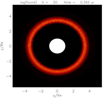
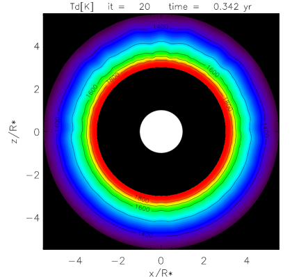
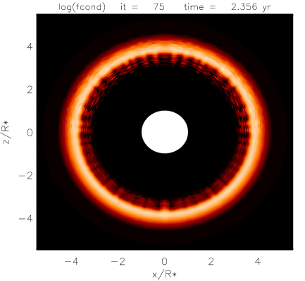
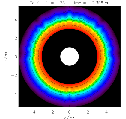
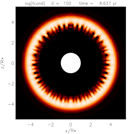
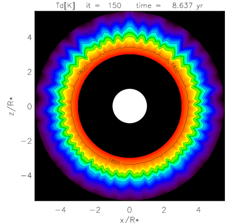
Figure 2: Self-organisation and spatio-temporal structure formation, triggered by radiative/thermal instabilities, during the formation of a dust shell around a carbon-rich AGB star. The figures show contour plots of the degree of condensation $\log(f_{\rm cond})$ (left column) and the dust temperature structure $T_{\rm d}$ (right column) in the $x$/$z$-plane (cut through the $y\!=\!0$-plane) at three selected time steps as indicated on top. On the r.h.s., black colour indicates regions that are not included in the model. The white circles in the centre of each figure mark the star. Because of axisymmetry, all data points appear twice at $\pm x$. Parameters: $T_{\rm eff}\!=\!3600\,$K, $L_{\star}\!=\!3000\,L_{\odot}$, $R_{\star}\!=\!9.79\cdot 10^{12}\,$cm, $\rm C/O\!=\!2$, $H_{\rho}\!=0.25\,R_{\star}$, $n_{\langle{\rm H}\rangle}(r_{0})\!=\!3.7\cdot\!10^{10}\,\rm cm^{-3}$ and $C_{2}\!=0.1/0.03$.

The results obtained from our axisymmetric model calculations are presented in the following way. We start by showing one exemplary model and explain the main physical processes in Sect. 3.1. The radial development of the dust is further discussed in Sect. 3.2 and the angular deviations from it (structure formation) in Sect. 3.3. Sect. 3.4 gives more insight into the nature of the radiative/thermal instability and discusses where the dust forming gas in an AGB star wind might be affected by this instability. The functional dependencies of the introduced parameters are outlined in Sect. 3.5 and Sect. 3.6 discusses the influence of the forming dust clumps on the spectral appearance of the star by means of calculated spectral energy distributions and monochromatic images.

3.1 One exemplary model

The development of the forming dust shell in a typical model, in terms of the degree of condensation $f_{\rm cond}(\@vec{r},t)$ and the dust temperature $T_{d}(\@vec{r},t)$, is shown in Fig. 2. The denser regions close to the star condense first, because the nucleation and growth of the dust particles proceeds faster at larger densities. Consequently, the spatial dust distribution, at first, resembles the slightly inhomogeneous gas distribution in the circumstellar shell with a cutoff at the inner edge as a consequence of the temperatures being too high for nucleation close to the star, and a smooth outer boundary due to the radially decreasing density. According to the different choice of the density inhomogeneities above/below mid-plane (see Eq. 30), the resulting spatial variations in the degree of condensation, $\Delta_{\theta}\log f_{\rm cond}$, are larger above than below the mid-plane at early phases of the model (see upper left plot in Fig. 2). Noteworthy, $\Delta_{\theta}\log f_{\rm cond}$ is larger than $\Delta_{\theta}\log n_{\langle{\rm H}\rangle}$, because the inverse dust formation time-scale initially scales with the density to a power of 3 … 4 (Woitke 2001).

The process of dust formation continues for a while in this way, until the first cells close to the star become optically thick. Each already optically thick cell casts a shadow into the circumstellar envelope wherein the temperatures decrease by several 100 K which improves the conditions for subsequent dust formation therein. At the same time, scattering and re-emission from the already condensed cells intensifies the radiation field inbetween. The stellar flux finally escapes preferentially through the segments which are still optically thin, thereby heating them up and worsening the conditions for further dust formation there. These two contrary effects amplify the initial spatial contrast of the degree of condensation introduced by the assumed density inhomogeneities. In the end, radially aligned, cool, linear dust structures, henceforth called dust fingers have developed, which point towards the star and are surrounded by warmer, almost dust-free regions at the inner edge of the forming dust shell. The lengths of the fingers is of the order of $0.5\,R_{\star}$.

3.2 The chemical wave

Apart from the self-organisation of the dust in the angular direction, the model reveals basically the formation and evolution of a radial dust shell. For a better visualisation of these processes, we have plotted several angle-averaged quantities $\langle X\rangle_{\theta}(r)$ in Fig. 3. The effective formation of dust generally requires a suitable combination of gas density and temperature, called the dust formation window (Gail${\rm\hskip 3.01385pt\&\hskip 3.01385pt}$Sedlmayr 1998). In the beginning of the model, favourable temperature conditions for efficient nucleation are only present in a restricted radial zone close to the star. However, as time passes, the dust shell becomes optically thick which dams the outflowing radiation and leads to a considerable increase of the temperatures inside of the shell (radiative backwarming). Consequently, the zone of effective dust formation shifts outward with increasing time. Moreover, the temperatures at the inner edge of the shell temporarily exceed the sublimation temperatures $T_{\rm S}$, and the dust shell begins to re-evaporate from the inside. The upper plot of Fig. 3 shows that $T_{\rm d}$ in fact temporarily exceeds its equilibrium value which is reached at later stages (see Sect. 3.4).

These two effects result in an apparent motion of the dust shell, driven by dust formation at the outer edge and dust evaporation at the inner edge of the shell, which will be denoted by chemical wave in the following. Chemical waves are a well-known phenomenon in the laboratory, for example the famous Belousov-Zhabotinsky reaction (Zaikin${\rm\hskip 3.01385pt\&\hskip 3.01385pt}$Zhabotinsky 1970), when chemical systems show oscillatory solutions, sometimes radiatively controlled (Schebesch${\rm\hskip 3.01385pt\&\hskip 3.01385pt}$Engel 1999), even without fluid bulk velocity fields. The apparent propagation velocity of the chemical wave, calculated from Fig. 3, decreases from $\approx\,2\rm\,km/s$ (early phase) to $\approx\,0.1\rm\,km/s$ (late phase).

Figure 4 shows more details of the structure of the chemical wave. The outer regions ahead of the wave are featured by a positive nucleation rate $J(a_{\ell})\!=\!J_{\star}\!>\!0$ and a positive growth time-scale $\tau_{\rm gr}>0$. In the centre of the wave, $f_{\rm cond}$ is maximum and $J(a_{\ell})$ and $1/\tau_{\rm gr}$ vanish. The layers behind the wave (close to the star) usually possess a negative flux through the size integration boundary $J(a_{\ell})\!<\!0$ and a negative growth time-scale $\tau_{\rm gr}<0$.

Figure 3: The chemical wave: formation and propagation of a dust shell via dust formation at the outer edge and dust evaporation at the inner edge. The figure shows the time evolution of the angle-averaged dust temperature $\langle T_{\rm d}\rangle_{\theta}(r)$ (upper plot) and degree of condensation $\langle f_{\rm cond}\rangle_{\theta}(r)$ (lower plot). The quantities are shown for iteration step ${\rm it}\!=\!0\,(t\!=\!0$, full), ${\rm it}\!=\!10\,(t\!=\!0.21\,$yr, dotted), ${\rm it}\!=\!20\,(t\!=\!0.36\,$yr, dashed), ${\rm it}\!=\!40\,(t\!=\!0.84\,$yr, dashed-dotted), ${\rm it}\!=\!70\,(t\!=\!2.1\,$yr, dashed-triple-dotted), ${\rm it}\!=\!120\,(t\!=\!5.7\,$yr, long-dashed) and ${\rm it}\!=\!195\,(t\!=\!13\,$yr, full).

Figure 4: Detailed radial snapshots of various angle-averaged quantities. Upper boxes: dust temperature $\langle T_{\rm d}\rangle_{\theta}$ (full line) and gas temperature $\langle T_{\rm g}\rangle_{\theta}$ (dashed). Second boxes: positive nucleation rate $\langle J_{\star}/n_{\langle{\rm H}\rangle}\rangle_{\theta}$ (full line) and negative evaporation rate $-\langle J(a_{\ell})/n_{\langle{\rm H}\rangle}\rangle_{\theta}$ (dashed). Third boxes: inverse growth time scale $\langle 1/\tau_{\rm gr}\rangle_{\theta}$. Lower boxes: degree of condensation $\langle f_{\rm cond}\rangle_{\theta}$. The errorbars indicate no errors but standard deviations $\Delta_{\theta}X$ of the angular variations of the calculated quantities $X(\@vec{r},t)$.

After the passage of the chemical wave, the system relaxes towards a stable equilibrium state, where the dust and the temperature structure of the medium are mutually coupled in a fine-tuned way. The equilibrium is enforced by a self-regulation mechanism: More dust causes an increase of the temperatures in the neighbourhood via backwarming, which leads again to dust evaporation and vice versa. This mechanism results in a physical state close to phase equilibrium $T_{d}\!\to\!T_{\rm S}$ (or, alternatively speaking, $\tau_{\rm gr}\!\to\!\infty$, see Sect. 2.2) for long times after the chemical wave has passed, featured by a considerable increase of $\langle f_{\rm cond}\rangle_{\theta}(r)$ and a moderate decrease of $\langle T_{\rm g}\rangle_{\theta}(r)$ with increasing $r$. The relaxation time-scale towards this equilibrium state is approximately given by the characteristic dust growth/evaporation time-scale, $|K_{3}/(dK_{3}/dt)|$, which is density-dependent. Limited by our explicit numerical iteration scheme, we are forced to keep the computational time-step $\Delta t$ smaller than this characteristic time-scale in the inner regions (see Sect. 2.6) which makes it computationally difficult to trace the chemical wave much further out, where the dust formation proceeds slower by orders of magnitude due to the lower densities.

3.3 Structure formation

Beside the evolution of the dust component in the $r$-direction, represented by angle-averaged quantities $\langle X\rangle_{\theta}(r)$, Fig. 4 shows the standard variations of angular variations of the calculated quantities by means of errorbars. These “errorbars” have nothing to do with real “errors”, but give an impression of the magnitude of the angular variations occurring in the model (compare also Fig. 2).

In general, the chemical wave is found to leave behind a strongly inhomogeneous dust distribution, where $f_{\rm cond}$ varies between zero and particular maximum values, which depend on the gas density and the distance to the star. From Fig. 4 (r.h.s.) we see that usually $\Delta_{\theta}X(r)\!>\!\langle X\rangle_{\theta}(r)$, where $X\!\in\!\{J(a_{\ell}),1/\tau_{\rm gr},f_{\rm cond}\}$, for long times after the passage of the chemical wave in the regions close to the star, i. e. the angular variations of all relevant dust quantities are usually larger than their mean values. This result is a complicate consequence of several factors.

• The dust formation process requires the formation of seed particles (nucleation), which depends exponentially on $T_{\rm g}$ with threshold character. Therefore, small temperature variations may result in large variations of the dust quantities.

• The dust growth rate is density-dependent. Small density variations temporarily lead to large contrasts of $f_{\rm cond}$ in early phases of the condensation process.

• The sublimation temperature $T_{\rm S}$ depends on the density. Denser regions are more resistant against thermal evaporation, because the partial pressures of carbon molecules in the gas phase are higher and hence the supersaturation ratio $S$ larger for larger gas densities.

• Radiative transfer effects introduce a non-local spatial coupling. In particular, dense cells with high $f_{\rm cond}$ cast shadows. In the shadowed regions behind these “clouds”, the conditions for the subsequent formation (nucleation) and the survival of the dust (thermal stability) are improved due to shielding effects.

The first two points lead to an inhomogeneous dust distribution already during early phases of the dust condensation process. As soon as the dust shell becomes optically thick, the backwarming enforces a partial re-evaporation of the dust, until the radiative energy finds ways to partly escape the system. Due to the threshold-like temperature-dependence of the dust survival, and the density-dependence of $T_{\rm S}$, the dust in the slightly denser cells close to the star just even survives, whereas the dust in the adjacent (slightly thinner) cells evaporates completely. Figure 4 shows that $1/\tau_{\rm gr}$ (zero indicates phase equilibrium) varies from slightly positive to considerable negative values behind the chemical wave, i. e. these regions consist of a mixture of cells where the dust is just even thermally stable and cells where all dust particles evaporate/have evaporated.

The spatial coupling via radiative transfer effects brings order into this chaos. If the dust in one particular cell can resist the radiation field, it shields the radiation and facilitates the survival of the dust in the shadow of this cell. Therefore, the final equilibrium state of the medium can in fact possess a non-trivial spatial structure, where cool, optically thick segments can coexist besides warmer, optically thin segments. The radiative flux finally escapes preferentially through these optically thin segments where the degree of condensation remains low (see upper right plot of Fig. 4). Thus, finger-like dust structures develop (see Fig. 2) which point toward the star.

3.4 The metastable region

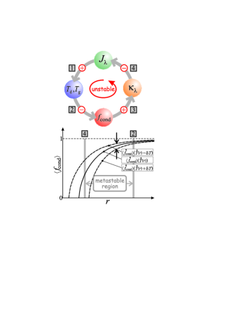
Figure 5: Sketch of the radiative/thermal instability of dust formation and related size of the metastable region.

The driving mechanism for the structure formation is an unstable physical control loop as thoroughly discussed in Paper I and once again sketched in the upper part of Fig. 5. The physical feedbacks [1] and [3] (temperature-dependence on radiation field and opacity-increase in case of condensation) are always positive and active. However, the feedback [2] diminishes at too low temperatures: Let ${\stackrel{{\hskip 1.50694pt{}_{\circ}}}{{f}}_{\rm cond}(r)}$ and ${\stackrel{{\hskip 0.3014pt{}_{\circ}}}{{T}}(r)}$ denote the degree of condensation and the dust temperature structure in the final equilibrium state reached long after the passage of the chemical wave. The ability of the medium to condense can then be expressed by ${\langle\stackrel{{\hskip 1.50694pt{}_{\circ}}}{{f}}_{\rm cond}\rangle}(T)$. At too low temperatures (large $r$), a small temperature change $\delta T$, e. g. by shadow casting, has only little influence on this quantity (as indicated by the vertical arrows in Fig. 5), the control loop is broken and an outer boundary of the metastable region results (see lower part of Fig. 5). On the other hand side, the feedback [4] (the non-local effect of opacity on the temperature structure, in particular shadow casting) requires that the medium is not completely optically thin, which creates an inner boundary of the metastable region. Here, the achievable degree of condensation is too small because of too high temperatures, and since gas opacities are unimportant, the medium cannot attain a considerable optical thickness.

Consequently, significant structure formation only occurs in a limited spatial zone of the model (see Fig. 2) between two boundaries, denoted by [4] and [2] in Fig. 5, henceforth called the metastable region. Here, the matter finally remains in a metastable state which is not fully condensed nor completely dust-free, where small fluctuations cause large effects.

From the numerical results, we infer that the size of this metastable region is essential for the significance of the forming dust structures. Only if this region is large, there is enough space for the radiative/thermal instability to bear in fact large-scale spatio-temporal structures. This size is related to the radial density gradient of the medium. With outward decreasing temperature, a certain radial gradient of the vapour pressure of the dust grain material $p_{\rm vap}\big{(}T_{\rm d}(r)\big{)}$ is given. If the gas density decreases with a similar gradient, the supersaturation ratio $S$ is of the order of unity in an extended radial zone.

3.5 Functional dependence on model parameters

This paragraph describes the influence of the model parameters on the structure formation process, based on the experience gained from other model calculations with different parameters not shown in detail in this paper. The numbers in squared brackets in the item list below are the parameter values of the standard model discussed so far (in Figs. 2, 3 and 4).

$T_{\rm eff}$  [$3600\rm\,K$]:

The effective temperature of the star triggers the mean radial distance of the dust formation zone. If $T_{\rm eff}$ is decreased, the metastable zone (see Sect. 3.4) is located closer to the star and results to be narrower, which leads to the formation of less significant dust structures.

$n_{\langle{\rm H}\rangle}(r_{0})$  [$3.7\cdot 10^{10}\,\rm cm^{-3}$]:

The gas density in the circumstellar environment is responsible for the dust growth time-scale and, hence, for the velocity of the chemical wave. By changing this parameter, the model mainly proceeds on a different time-scale. Larger densities also lead to an increase of $T_{\rm S}$, which means that the formation and the survival of dust is already possible closer to the star. Furthermore, larger densities potentially lead to the formation of more dust on an absolute scale, which produces larger optical depths. In models with strongly reduced $n_{\langle{\rm H}\rangle}(r_{0})$, the resulting optical depths are too small to cause significant temperature changes via backwarming and shadow formation, and the system decouples spatially, i. e. every cell condenses on its own, without much feedback on the neighbouring cells. In models with larger $n_{\langle{\rm H}\rangle}(r_{0})$, we observe that only slightly larger optical depths occur as compared to the standard model, but that the dust shell is narrower. This is a consequence of the re-evaporation process which sets in as soon as a certain critical value of $\tau_{\rm 1\mu m}$ is reached (here about $1\,...\,3$). The temperatures temporarily reach higher values behind the wave as depicted in Fig. 3 and the dust evaporation is faster and more complete on the inside of the shell. In both cases of varied $n_{\langle{\rm H}\rangle}(r_{0})$, less pronounced structure formation is found to occur.

$\rm C/O$  [$\rm 2.0$]:

The initial carbon-to-oxygen ratio is a measure for the amount of condensable material in the gas. Consequently, changing C/O has a similar influence than changing the overall density level by means of $n_{\langle{\rm H}\rangle}(r_{0})$.

$H_{\rho}$  [$0.25\,R_{\star}$]:

The scale height is important for the radial extension of the metastable zone (see Sect. 3.4). We observe from models with larger $H_{\rho}$ that the size of the metastable zone is smaller and, consequently, the structure formation results to be less significant. However, even for models with $n_{\langle{\rm H}\rangle}\!\propto\!1/r^{2}$, where the density gradient is much shallower, some structures still develop.

$C_{2}$  [$0.1/0.03$]:

The degree of density inhomogeneities (see Eq. 28) is not a critical parameter of the model ! From Fig. 2 we see that the number and the shape of the dust structures is finally similar above and below the mid-plane, despite the different values for $C_{2}$. The finger-like structures even develop for $C_{2}\!=\!0$. For larger density inhomogeneities, the structures become slightly longer and less numerous.

Spatial resolution  [$71\times 71$ grid points]:

The number of radial grid points in the model is important for the proper resolution of the radiative transfer and the propagation velocity of the chemical wave. The number of angular grid points is crucial with respect to the shape and, in particular, the width of the resulting dust structures. In the depicted model (Fig. 2), $N_{\rm struc}\!=\!27$ dust structures can be identified within $N_{\theta}+1\!=\!71$ angular grid points, i. e. the resulting number and width of the dust fingers is at the limit of the angular resolution of the model.

The resulting width of the dust fingers is possibly a consequence of the way how we have introduced the density inhomogeneities in our model. Using random numbers for all cells (see App. A), the resulting density inhomogeneities are spatially uncorrelated and the characteristic scale of the density variations is naturally given by the size of the cells, which is apparently important for the width of the dust fingers. We have run model calculations with up to 181 angular grid points (which forces us to reduce $N_{r}$ to 40 due to computer memory and time-consumption limitations), where the finger-like dust structures become narrower at the head and slightly conic according to the shape of the penumbra. The ratio $N_{\rm struc}/N_{\theta}$ becomes less if $N_{\theta}$ is increased. However, definite predictions about the diameter of the dust structures are difficult to make, because of the limited angular resolution in our model.

3.6 Spectral appearance

From an observational point of view, it is interesting to discuss how a “clumpy” dust distribution around an AGB star would appear both spectroscopically and in monochromatic images. Figure 6 shows the calculated spectral energy distribution (SED) of the standard model at the end of the computation. The depicted flux has been averaged over all escape directions $\theta_{\rm esc},\phi_{\rm esc}$ (see Niccolini${\rm\hskip 3.44444ptet\hskip 3.01385ptal.\hskip 2.58334pt}$2003). The resulting SED is featureless according to the amorphous carbon opacities and can reasonably well be fitted by a black body with colour temperature $\approx 2700\,{\rm K}\,...\,2900\,$K (note the difference to the effective temperature $T_{\rm eff}\!=\!3600\,$K).

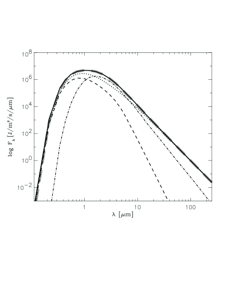
Figure 6: Calculated spectral energy distribution of the clumpy model at $t\!=\!13.2\,$yr, averaged over all escape directions. Flux values correspond to a distance of $1\,R_{\star}$. Full line: calculated total flux, dotted line: direct star light, thin dashed line: scattered star light, dashed-dotted line: thermal dust emission (partly scattered), thick grey dashed line: total flux of a spherically symmetric reference model (see text).

The Monte Carlo method allows for an identification of the kind of photons which reach the observer. The optical (blue) part of the spectrum mainly results from direct star light, which is attenuated by dust extinction, and from multiply scattered star light. The near IR spectral region around $2\,\mu{\rm m}\,...\,4\,\mu$m is dominated by thermal dust emission, whereas for longer wavelengths, the dust envelope becomes optically thin and the direct star light again becomes the most important contributor.

To our surprise, the resulting angle-averaged SED contains almost no evidence for the clumpy dust distribution in the model, contrary to what results from simplified models for spectral analysis (e. g. Jørgensen${\rm\hskip 3.44444ptet\hskip 3.01385ptal.\hskip 2.58334pt}$2000). We have calculated a time-dependent reference model which is identical to the standard model, except for a choice of $N_{\theta}=1$, i. e. all “cells” are closed spherical shells in the reference model, which enforces the results to be spherically symmetric. Figure 6 shows that the calculated SED of the “clumpy” standard model is practically indistinguishable from the SED of this reference model at an comparable instant of time. There is only a slight excess in the blue part of the spectrum as compared to the reference model (e. g. +15% at $\lambda\!=\!0.34\,\mu$m, +4% at $\lambda\!=\!0.55\,\mu$m, +1% at $\lambda\!=\!0.72\,\mu$m), caused by the increased average escape probability in the blue in case of a clumpy medium.

Table 2: Comparison of the standard “clumpy” model to a spherically symmetric reference model at $t\!=\!13.2\,$yr (see text). $\langle T_{\rm d}\rangle_{M_{\rm d}}$ is the mass-averaged dust temperature and $\tau_{1\mu\rm m}$ the radial optical depths at $\lambda\!=\!1\,\mu$m.

	clumpy model	reference model
$M_{\rm gas}\,[M_{\odot}]$	$1.35\cdot 10^{-6}$	$1.35\cdot 10^{-6}$
$M_{\rm dust}\,[M_{\odot}]$	$5.23\cdot 10^{-10}$	$4.69\cdot 10^{-10}$
$\tau_{1\mu\rm m}$	$0.51\,\ldots\,2.7$	0.98
$T_{\star}\rm\,[K]$	$3610.7$	$3610.6$
$\langle T_{\rm d}\rangle_{M_{\rm d}}\rm\,[K]$	$1638$	$1654$

Table 2 shows more details about this comparison. In fact, about 10% more dust (by mass) condenses in the standard model as compared to the spherically symmetric reference model. The standard deviation of the optical depth at $\lambda\!=\!1\,\mu$m is larger than its mean value $\langle\tau_{1\mu\rm m}\rangle$. The mass-averaged dust temperature $\langle T_{\rm d}\rangle_{M_{\rm d}}=\big{(}\sum_{\xi}V_{\xi}\,n_{\langle{\rm H}\rangle}^{\xi}\widehat{K}_{3}^{\,\xi}\,T_{\rm d}^{\,\xi}\big{)}\big{/}\big{(}\sum_{\xi}V_{\xi}\,n_{\langle{\rm H}\rangle}^{\xi}\widehat{K}_{3}^{\,\xi}\big{)}$ is slightly lower than in the reference model, where $V_{\xi}$ is the volume of cell $\xi$. In summary, if the assumption of spherical symmetry is relaxed to axisymmetry, more dust condenses in the stellar environment which forms and survives in radiatively shielded, cool clumps, resulting in a lower mean dust temperature. However, the characteristic changes are only of the order of 10%, and it is noteworthy that the different single effects tend to compensate each other in view of the spectral appearance.

direct dust emission	scattered dust emission
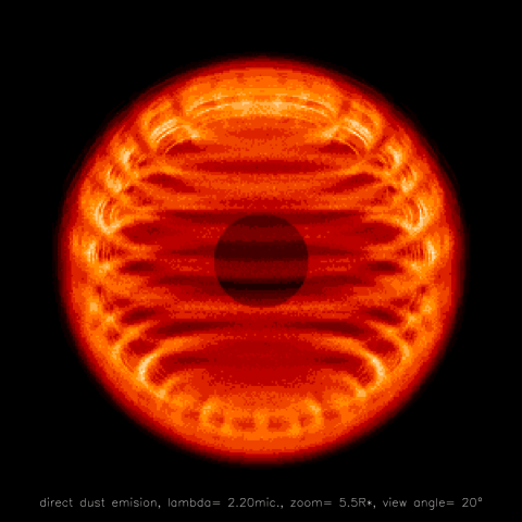
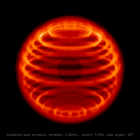
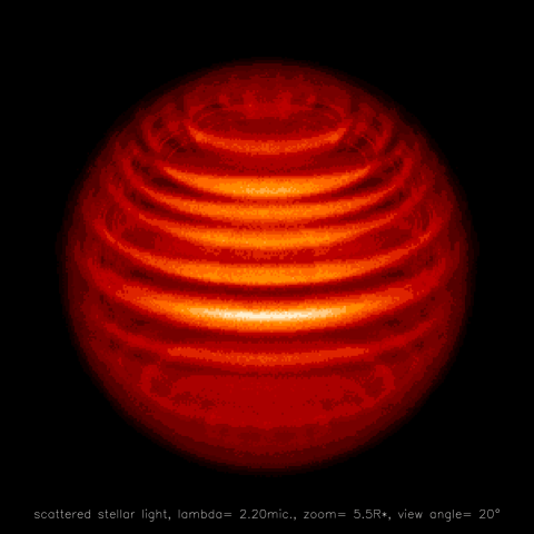
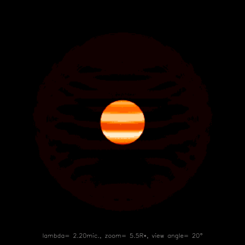
scattered star light	total

Figure 7: Simulated images at 2.2 $\mu$m for an inclination angle of $20^{\circ}$ between the equator and the observer’s direction of the innermost $\pm 4.5\,R_{\star}$ of the model. The dust distribution refers to the final state of the model ($t\!=\!18.4\,$yr). The total signal is shown in the lower right plot, whereas the other (artificial) images show the different constituents of the signal (total = direct star light + scattered star light + direct dust emission + scattered dust emission). Note the different scaling of the intensities, given in units of $\rm 10\,W\,m^{-2}\mu{m}^{-1}$ for a reference distance of $1\,R_{\star}$. The picture of the direct star light is very similar to the total signal depicted on the lower rights, and is hence omitted.

From Fig. 6, we can infer that the spectral region around $2\,\mu{\rm m}\,...\,4\,\mu$m, which approximately coincides with the maximum of the thermal emission from the dust envelope, is most promising to reveal the spatial dust distribution around the star by direct imaging. Figure 7 shows simulated pictures at $\lambda\!=\!2.2\,\mu$m. The light from the dust shell mainly arises from the glowing heads of the dust fingers, which appear as rings around the star due to our assumption of axisymmetry. The different physical contributions are shown separately in Fig. 7. However, the intensities received from the dust shell are about one order of magnitude less than the intensities received from the star. The lower right image depicts the total brightness distribution, where basically only a stellar disk is visible, which is partly obscured by the inhomogeneous dust distribution around the star.

Observations of such non-uniformly bright stellar disks are usually explained by cool and/or hot spots on the stellar surface, e. g. in case of the cool supergiant $α$~Ori (Lynds${\rm\hskip 3.44444ptet\hskip 3.01385ptal.\hskip 2.58334pt}$1976, Gilliland${\rm\hskip 3.01385pt\&\hskip 3.01385pt}$Dupree 1996). However, an inhomogeneous dust distribution around the star (which is a perfectly uniform black body sphere in our model) can obviously lead to a similar optical appearance, even if there is not much direct evidence for dust in the image. Thus, the interpretation of monochromatic images, e. g. by speckle interferometry, via cool and hot spots on the stellar surface is delicate if there is only the slightest evidence for the existence of circumstellar matter, e. g. by spectroscopy, which could be inhomogeneous.

In fact, the direct + scattered star light only provides $\approx\!40\%\!+\!8\%$ of the total signal integrated over the entire image, whereas $\approx\!37\%\!+\!15\%$ originates from the dust envelope (direct + scattered dust emission). However, the dust emission is spread over a much more extended area, here $\sim\!\pi(4\,R_{\star})^{2}$, than the direct star light $\sim\!\pi R_{\star}^{\,2}$. Consequently, the intensities received from the dust envelope are generally much weaker than the intensities received from the stellar disk (factor $\sim\!16$).

The different physical contributions to the image are separately shown in Fig. 7. A composite picture of scattered star light + direct dust emission + scattered dust emission (lower left + upper left + upper right in Fig.7) would simulate a coronographic image where the stellar disk is blinded out. Such observations could in fact reveal the spatial dust distribution around the star. Of course, since our model is axisymmetric, the “clumpy” dust distribution in the model appears as superposition of rings in the image, which is not expected to be realistic. Nevertheless, the images give a first impression of the kind of brightness distributions to be expected from a cloudy circumstellar environment.

4 Conclusions and discussion

This paper has shown that the formation of dust shells in the circumstellar environments of late-type stars can be unstable. Spontaneous symmetry breaking may occur due to a radiative/thermal instability in the dust forming gas, which leads to the development of cloud-like dust structures close to the star.

These results have been obtained on the basis of time-dependent axisymmetric models, which combine a kinetic description of carbon dust formation/evaporation with detailed, frequency-dependent radiative transfer by means of a Monte Carlo method, in the static case. The simulations show that the dust preferentially forms behind already condensed regions, which shield the stellar radiation. In the shadow of these clumps, the temperatures are lower by a few 100 K which triggers the subsequent formation and facilitates the survival of the dust close to the star. As final result, numerous finger-like dust structures develop which may have an radial extension as large as $0.5\,R_{\star}$ and point towards the centre of the radiant emission, similar to the “cometary knots” observed in planetary nebulae and star formation regions.

The cloudy dust distribution has little effect on the calculated spectral energy distribution of the star, in comparison to a spherically symmetric model, but significantly influences the optical appearance of the circumstellar environment in near IR monochromatic images (e. g. at $\lambda\!=\!2.2\,\mu$m). In particular, an inhomogeneous dust distribution around the star leads to a likewise non-uniformly bright appearance of the stellar disk. Comparable observations of late-type giants are commonly interpreted in terms of hot/cool spots on the stellar surface. However, our model suggests that a different physical explanation by dust is possible for these observations, even if the dust is barely visible in the image.

Due to computational time constraints, we have so far only been able to study the static case where velocity fields are ignored. In this case, the main feature of the model is the formation of a chemical wave which radially propagates outward, driven by dust formation on the outer edge and dust evaporation due to backwarming at the inner edge. The optical depth of this chemical wave reaches about $\tau_{\rm 1\mu m}\!\la\!1\,...\,3$ with a density-dependent propagation velocity of $\approx\!0.1\rm\,km/s\,...\,2\rm\,km/s$. The wave leaves behind a strongly inhomogeneous dust distribution close to the star, where the medium relaxes towards phase equilibrium. However, this process is unstable and results in the aforementioned simultaneous occurrence of cool dusty (optically thick) segments beside warmer, almost dust-free (optically thin) segments, through which the radiative flux finally escapes preferentially.

According to dynamical (but spherically symmetric) models of dust-forming AGB stars (e. g. Winters${\rm\hskip 3.44444ptet\hskip 3.01385ptal.\hskip 2.58334pt}$2000, Schirrmacher${\rm\hskip 3.44444ptet\hskip 3.01385ptal.\hskip 2.58334pt}$2003, Höfner${\rm\hskip 3.44444ptet\hskip 3.01385ptal.\hskip 2.58334pt}$2003, Sandin & Höfner 2003), the formation of dust mainly occurs in particular phases of the model triggered by the pulsation of the star, which results in radial dust shells. During such a dust shell formation phase, the effect of a re-evaporation from the inside is a typical feature, similar to the behaviour of our chemical wave. According to the present paper, this process should be unstable and might result in departures from spherical symmetry.

We believe that this instability can provide a basis for a better understanding of inhomogeneous dust distributions showing up in many observations. However, direct predictions for particular objects are difficult to make, because hydrodynamics is missing in the current model. Since the dust is blown away as soon as it forms, the system has only little time to relax towards phase equilibrium at the inner edge of the dust shell. On the one hand, this time may be too short to produce well-grown spatial dust structures as shown in this paper. On the other hand, even small deviations from spherical symmetry may trigger important dynamical effects, e. g.

• The radiation pressure on dust grains, which is delivered to the gas via frictional forces, mainly depends on the radiative flux and the degree of condensation. If slightly more condensed regions exist, they might be accelerated outward, whereas less condensed regions stay behind or even fall back.

• Optically thick dust clouds will be confined by radiation pressure, because the bolometric radiative flux is larger at the inner edge of the cloud facing the star than at its self-shielded outer edge (this effect does not occur in spherically symmetric models where $r^{2}F(r)=\rm const$ in radiative equilibrium). Driven, pancake-like structures could evolve due to this effect.

• The hydrodynamical process of cloud acceleration due to radiation pressure is not well-studied, apart from the special case of spherical symmetry. This process may be dynamically unstable itself (e. g. Rayleigh-Taylor, Kelvin-Helmholtz). Velocity disturbances generated by these instabilities may have an important feedback on the dust forming medium.

Thus, we propose a new hypothetical scenario for dust-driven AGB star winds: Excited by hydrodynamical, radiative or thermal instabilities, dust clouds are formed from time to time close to the star in temporarily shielded areas, which are accelerated outward by radiation pressure. At the same time, thinner, dust-free matter falls back towards the star at different places. A highly dynamical and turbulent environment close to the star would be created in this way, which can be expected to bear again a strongly inhomogeneous dust distribution.

In order to verify this hypothetical scenario, much more elaborate model calculations would be required which may well exceed the present capabilities of parallel super-computers. Various processes must be traced in 3D, using dynamical models with detailed radiative transfer and time-dependent dust-chemistry.

Appendix A Spatial grid

Figure 8: Spatial grid of the axisymmetric model. Each cell is a torus which appears twice (at $x\!>\!0$ and $x\!<\!0$) in this cut through the $y\!=\!0$ plane. Blank regions are not included in the model volume (the photons are assumed to pass through these regions). The star is indicated as central disc.

The model volume is subdivided into fixed spatial cells, where the cell boundaries are specified in spherical coordinates $r$, $\theta$ and $\phi$, using prescribed sampling points for the radius and the latitude angle, $r_{n}$ and $\theta_{k}$, respectively. A cell is the volume defined by the following coordinate intervals

$$r \in [r_{n-1},r_{n}]\;\;n=1,\,...\,,N_{r}$$ (25)

$$\theta \in [\theta_{k-1},\theta_{k}]\;\;\,k=1,\,...\,,N_{\theta}$$ (26)

$$\phi \in [0,2\pi]\ .$$ (27)

According to Eq. (27) the cells are closed tori, i. e. the model is axisymmetric (2D). Each cell is specified by one radial and one angular index, $n$ and $k$, respectively, which are abbreviated by a multi-index $\xi=(n,k)$. For the model discussed in detail in this paper, we choose a radial grid with $N_{r}+1\!=\!71$ logarithmic equidistant sampling points between $r_{0}/R_{\star}\!=\!3.0$ and $r_{N_{r}}/R_{\star}\!=\!5.5$ and $N_{\theta}+1\!=71$ equidistant angular grid points between $\theta_{0}\!=0$ and $\theta_{N_{\theta}}\!=\pi$. The spatial grid is visualised in Fig. 8.

The prescription of the density structure in the model volume (Eq. 1) is technically realised in each cell $\xi$ via

$$n_{\langle{\rm H}\rangle}^{\,\xi}=C_{1}\cdot\exp\left(-\frac{\bar{r}^{\,\xi}}{H_{\rho}}+C_{2}\cdot Z\right)\ ,$$ (28)

where $\bar{r}^{\,\xi}\!=\!(r_{n-1}\!+\!r_{n})/2$ the mean radial distance of cell $\xi$ and $Z$ a random number with Gaussian distribution and unity variance

$$Z=\sqrt{-2\ln(1-z_{1})}\cdot\sin(2\pi\,z_{2})\ .$$ (29)

$z_{1},z_{2}\in[0,1)$ are equally distributed pseudo random. $C_{1}\!=\!6\cdot 10^{15}\,\rm cm^{-3}$ is a constant chosen to produce the desired mean hydrogen nuclei particle density at the innermost radial grid point $n_{\langle{\rm H}\rangle}(r_{0})$. In order to study the influence of the assumed level of density inhomogeneities, we choose the second constant as

$$C_{2}=\left\{\begin{array}[]{ccl}0.10&,&\mbox{above mid-plane}\\ 0.03&,&\mbox{below mid-plane}\ .\end{array}\right.$$ (30)

The standard deviation of the density at constant radius, $\Delta_{\theta}\log n_{\langle{\rm H}\rangle}$, is $10\%\cdot\log{\rm e}\!\approx\!4.3\%$ above and $3\%\cdot\log{\rm e}\!\approx\!1.3\%$ below the mid-plane of the model volume ($z\!=\!0$).

References

- (1) Anders E., Grevesse N., 1989, Geochimica et Cosmochimica Acta 53, 197–214
- (2) Andersen A. C., Höfner S., Gautschy-Loidl R., 2003 A&A 400, 981–992
- (3) Bohren C. F., Huffman D. R., 1983, Absorption and Scattering of Light by Small Particles, John Wiley & Sons, New York
- (4) Chase Jr. M. W., Davies C. A., Downey Jr. J. R., Frurip D. J., McDonald R. A., Syverud A. N., 1985, JANAF Thermochemical Tables, National Bureau of Standards
- (5) Cherchneff I., Barker J. R., Tielens A. G. G. M., 1992, ApJ 401, 269–287
- (6) Diamond P. J., Kemball A. J., 2003, ApJ 599, 1372–1382
- (7) Dominik C., Gail H.-P., Sedlmayr E., 1989, A&A 223, 227–236
- (8) Feast M. W., Whitelock P. A., Marang F., 2003, MNRAS 346, 878–884
- (9) Fleischer A. J., Gauger A., Sedlmayr E., 1995, A&A 297, 543
- (10) Freytag B., Höfner S., 2003, poster contribution at International Scientific Meeting of the Astronomische Gesellschaft, September 15-19, 2003, Freiburg, Germany, AG abstract series 20
- (11) Gail H.-P., Sedlmayr E., 1987, A&A 171, 197–204
- (12) Gail H.-P., Sedlmayr E., 1988, A&A 206, 153–168
- (13) Gail H.-P., Sedlmayr E., 1998, In Sarre P., Chemistry and physics of molecules and grains in space. Faraday Discussion no. 109, 303, London, GB
- (14) Gail H.-P., Keller R., Sedlmayr E., 1984, A&A 133, 320–332
- (15) Gauger A., Gail H.-P., Sedlmayr E., 1990, A&A 235, 345–361
- (16) Gilliland R. L., Dupree A. K., 1996, ApJL 463, L29–L32
- (17) Haniff C. A., Buscher D. F., 1998, A&A 334, L5–L8
- (18) Heske A., Te Lintel Hekkert P., Maloney P., 1989, A&A 218, L5–L8
- (19) Jeong K. S., 2000, PhD thesis, Technische Universität, Berlin, Germany
- (20) Höfner S., Gautschy-Loidl R., Aringer B., Jørgensen U. G., 2003, A&A 399, 589–601
- (21) Jørgensen U. G., Hron J., Loidl R., 2000, A&A 356, 253–266
- (22) Jura M., Chen C., Plavchan P., 2002, ApJ 569, 964–974
- (23) Krüger D., Woitke P., Sedlmayr E., 1995, A&AS 113, 593–602
- (24) Lopez B., 1999, In Le Bertre T., Lèbre A., Waelkens C., IAU Symp. 191: AGB stars, 409–418. ASP
- (25) Lucy L. B., 1999, A&A 345, 211–220
- (26) Lynds C. R., Worden S. P., Harvey J. W., 1976, ApJ 207, 174–180
- (27) Niccolini G., Woitke P., Lopez B., 2003, A&A 399, 703–716
- (28) O’Dell C. R., 2000, AJ 119, 2311–2318
- (29) Olofsson H., Bergman P., Lucas R., Eriksson K., Gustafsson B., Bieging J. H., 2000, A&A 353, 583–597
- (30) Patzer A. B. C., Gauger A., Sedlmayr E., 1998, A&A 337, 847–858
- (31) Patzer A. B. C., Chang Ch., Sedlmayr E., Sülzle D., 2003, A&A submitted
- (32) Redman M., Viti S., Cau P., Williams D., 2003, MNRAS 345, 1291–1296
- (33) Rouleau F., Martin P. G., 1991, ApJ 377, 526–540
- (34) Sandin C., Höfner S., 2003 A&A 404, 789–807
- (35) Schebesch I., Engel H., 1999, Phys. Rev. E 60, 6429–6434
- (36) Schirrmacher V., Woitke P., Sedlmayr E., 2003, A&A 404, 267–282
- (37) Schröder K.-P., Winters J. M., Sedlmayr E., 1999, A&A 349, 898–906
- (38) Tuthill P., Monnier J., Danchi W., Lopez B., 2000, ApJ 543, 284–290
- (39) Weigelt G., Balega Y., Blöcker T., Fleischer A. J., Osterbart R., Winters J. M., 1998, A&A 333, L51–L54
- (40) Winters J. M., Le Bertre T., Jeong K. S., Helling Ch., Sedlmayr E., 2000, A&A 361, 641–659
- (41) Wiscombe W. J., 1980, Appl. Opt. 19, 1505–1509
- (42) Woitke P., 1999, In Diehl R., Hartmann D., Astronomy with Radioactivities, 163–174, MPE Report 274, Schlos Ringberg, Germany
- (43) Woitke P., 2001, Reviews in Modern Astronomy 14, 185–207
- (44) Woitke P., Sedlmayr E., Lopez B., 2000, A&A 358, 665–670
- (45) Zaikin A. N., Zhabotinsky A. M., 1970, Nature 225, 535