Escaping the Big Rip?

Abstract

We discuss dark energy models which might describe effectively the actual acceleration of the universe. More precisely, for a 4-dimensional Friedmann-Lemaître-Robertson-Walker (FLRW) universe we consider two situations: First of them, we model dark energy by phantom energy described by a perfect fluid satisfying the equation of state $P=(\beta-1)\rho$ (with $\beta<0$ and constant). In this case the universe reaches a “Big Rip” independently of the spatial geometry of the FLRW universe. In the second situation, the dark energy is described by a phantom (generalized) Chaplygin gas which violates the dominant energy condition. Contrary to the previous case, for this material content a FLRW universe would never reach a “big rip” singularity (indeed, the geometry is asymptotically de Sitter). We also show how this dark energy model can be described in terms of scalar fields, corresponding to a minimally coupled scalar field, a Born-Infeld scalar field and a generalized Born-Infeld scalar field. Finally, we introduce a phenomenologically viable model where dark energy is described by a phantom generalized Chaplygin gas.

I Introduction

Several astronomical and cosmological observations, ranging from the cosmic microwave background anisotropy Spergel:2003cb to observation of distant supernova Riess:1998cb , show that the universe is undergoing an accelerating stage. In addition, these observations show that the acceleration of the universe is due to some unknown stuff usually dubbed dark energy (DE), which constitutes roughly two thirds of the total energy density of the universe. Moreover, it is known that the DE satisfies an equation of state $P=(\beta-1)\rho$, where $|\beta|<0.3$ (at least recently in the history of the universe) Jimenez:2003nz .

So far, several phenomenological models have been proposed to describe the dark energy, being the cosmological constant, $\Lambda$, by far the most simple and popular candidate Lambda . However, this possibility is ruled out (in principle) as a consequence of the huge discrepancy between the expected theoretical and experimental value of $\Lambda$. A positive cosmological constant might describe the acceleration of the universe as it could be described as a perfect fluid with negative pressure, $-\Lambda$, and this is one of the main ingredients to produce an accelerating universe. In fact, a Friedmann-Lemaître-Robertson-Walker (FLRW) universe undergoes an accelerated stage as long as $\rho+3P<0$, where $\rho$ and $P$ correspond, respectively, to the total energy density and pressure of the matter content. Matter contents with this requirement can be described effectively, for example, by a perfect fluid; with a barotropic equation of state or a more exotic one like in (generalized) Chaplygin gas models chaplygin ; chaplygin2 ; MBL-PVM , or by dynamical scalar fields as in quintessence models quintessence and phantom energy models caldwell ; SSD ; phantom1 ; Li ; phantom2 ; phantom3 .

If dark energy would be described by either of the last two models mentioned above, then the future of the universe might be quite different. While for a quintessence scalar field, with an effective equation of state $P=(\beta-1)\rho$, with $\beta$ constant and $0<\beta<{2}/{3}$, dominating the energy density of the universe, the universe would expand forever, for a phantom energy; i.e. $\beta<0$, this might not be the case. In fact, for a matter content with a barotropic equation of state formally similar to the previous one, but with a negative $\beta$, the universe would experiment a cosmic doomsday, also dubbed big rip, phantom1 ; caldwell ; SSD ; Li ; phantom2 ; phantom3 ; i.e. the scale factor would blow up in a finite cosmic time. The last affirmation is based on a constant negative value of $\beta$. However, the value of $\beta$ may change along the evolution of the universe and then in principle the universe might not reach a big rip in the future.

Another candidate to describe dark energy is a (generalized) Chaplygin gas chaplygin , already mentioned, which corresponds to a perfect fluid with a rather strange equation of state $P=-A/\rho^{\alpha}$, where $A$ is a positive constant and $\alpha$ a parameter. This fluid can describe a transition from a dust dominated universe at early time to a de Sitter universe at late time. In addition, this matter content has been proposed as a unification of dark matter and dark energy. In this paper, we will show that if the dark energy is modelled by a phantom generalized Chaplygin gas, then the universe will escape the big rip and will expand forever. Others phantom energy models; i.e. matter contents with $\rho+P<0$ and a positive energy density, exhibiting similar property has already been proposed SSD ; Li . For example, this can be achieved considering a homogeneous minimally coupled scalar field with an appropriate potential SSD or with a Born-Infeld homogeneous scalar field Li . However, in these models, the scalar field has the wrong kinetic energy. In this paper, we propose an alternative phenomenological model to describe phantom energy by means of a fluid which, firstly, satisfies the generalized Chaplygin gas equation of state chaplygin , and secondly, violates the dominant energy condition EllisHawking . Moreover, for this peculiar material content a FLRW universe would never reach a Big Rip.

The paper can be outlined as follows. In the next section, on the one hand, we will review the phantom energy model with a constant equation of state ($\beta$ is negative and constant) in FLRW universes, giving the explicit expression of the scale factor for the three different spatial geometries. On the other hand, we will discuss if the presence of a positive cosmological constant might alleviate the big rip problem. In section III, we introduce and study a dark energy model based on a generalized Chaplygin gas. In section IV, we analyze our model in the light of scalar fields, corresponding to a minimally coupled scalar field, a Born-Infeld scalar field and a generalized Born-Infeld scalar field. In section V, we describe a phenomenologically viable model, where the dark energy is described by a phantom generalized Chaplygin gas. Finally, we briefly summarize and discuss our results in section VI.

II Phantom energy

Through the paper, we mainly consider the late time evolution of a homogeneous and isotropic universe. Furthermore, we model dark energy by phantom energy, which in the present section is described by a perfect fluid satisfying the equation of state $P=(\beta-1)\rho$, where $\beta$ is constant and negative. The conservation equation results on $\rho=\tilde{A}a^{-3\beta}$, where $\tilde{A}$ is an integration constant. Therefore, for $\beta<0$ the energy density grows with the scale factor instead of decreasing. For simplicity, we disregard the other matter contents of the universe as their energy densities decrease with the cosmic time and can be neglected in comparison with the energy density of phantom matter at very late time when a big rip could happen . Consequently, the Friedmann equation can be expressed as

$$H^{2}+\frac{k}{a^{2}}=\frac{8\pi\textrm{G}}{3}\tilde{A}a^{-3\beta},$$ (1)

where $H$ is the Hubble constant and $k=1,-1,0$, corresponding to spherical, hyperbolic or flat spatial sections of the FLRW model.

For flat spatial section ($k=0$) the scale factor scales with the cosmic time, t, as

$$a(t)=\left[a_{0}^{3\beta/2}+\frac{3\beta}{2}C^{1/2}(t-t_{0})\right]^{2/(3\beta)},$$ (2)

where $a_{0}$ and $t_{0}$ will be integration constants throughout the paper, corresponding to the initial radius and cosmic time of the universe and $C=(8\pi\textrm{G}/3)\tilde{A}$. As can be seen, for negative $\beta$, the scale factor diverges in a finite cosmic time

$$t_{\infty 0}=t_{0}-\frac{2}{3\beta C^{1/2}}a_{0}^{3\beta/2},$$ (3)

if $t$ varies between $t_{0}$ and $t_{\infty 0}$. Therefore, the universe would reach a cosmic doomsday caldwell . For values of the cosmic time larger than $t_{\infty 0}$ the scale factor will decrease until vanishing at $t\rightarrow+\infty$. It can also be seen that when $\beta$ approaches zero, $t_{\infty 0}$ goes to infinity. A similar situation can be found in the case of a FLRW universe with hyperbolic or spherical spatial geometry [see Fig. 1]. This is not surprising as for a vanishing $\beta$, the FLRW geometry corresponds to a de Sitter space-time sliced into flat sections and there is no longer a big rip. In addition, for a given initial value of the scale factor $a_{0}>\exp[2/(3\beta)]$, the larger is the value of $\beta$, the larger is the value of $t_{\infty 0}$ at which the big rip happens. Moreover, the latter the phantom energy starts dominating the energy density of the universe; i.e. the larger the value of $a_{0}$, the sooner the universe reaches the big rip.

In the spherical case ($k=1$), the scale factor must be larger than $a_{\textrm{min}}=C^{1/(3\beta-2)}$. Otherwise, the Friedmann equation (1) is not well defined. We have that the cosmic time scales with the scale factor as W

$$t-t_{0} = \frac{2C^{1/(3\beta-2)}}{2-3\beta}\;\left({Ca^{2-3\beta}-1}\right)^{1/2}$$ (4)

$$\times \textrm{F}\left(\frac{3\beta-1}{3\beta-2},\frac{1}{2};\frac{3}{2};1-Ca^{2-3\beta}\right),$$

where $\textrm{F}(b,c;d;e)$ is a hypergeometric series W . The cosmic time is finite whenever $-1\leq 1-Ca^{2-3\beta}\leq 0$, i.e. $a_{\textrm{min}}\leq a\leq\left(2/C\right)^{1/(2-3\beta)}$. For larger values of the scale factor the expression (4) breaks down and, consequently, we cannot immediately conclude either the existence or the absence of a cosmic doomsday. However, the difference between the cosmic times corresponding, respectively, to $t_{\infty+}$ when the scale factor blows up, and to a given cosmic time $t$ such that $a(t)$ is larger than $\left(2/C\right)^{1/(2-3\beta)}$ can be expressed as follows

$$t_{\infty+}-t=-\frac{2C^{1/(3\beta-2)}}{3\beta}\;\left({Ca^{2-3\beta}-1}\right)^{-\frac{3\beta}{2(3\beta-2)}}$$

$$\times \textrm{F}\left(\frac{3\beta-1}{3\beta-2},\frac{3\beta}{2(3\beta-2)};\frac{3\beta}{2(3\beta-2)}+1;\frac{1}{1-Ca^{2-3\beta}}\right).$$

In addition, it can be checked that the last expression is well defined, in particular the hypergeometric function (see footnote 4), whenever $a$ is larger or equal than $\left(2/C\right)^{1/(2-3\beta)}$. This value of the scale factor corresponds precisely to the maximum value allowed in Eq. (4). Consequently, we can conclude that there is a big rip in a FLRW universe sliced into spherical sections filled with phantom matter when $\beta$ is constant and negative. In this case, we have that the cosmic time elapsed since the scale factor acquires its minimum value $a_{\textrm{min}}$ at $t=t_{0}$ up to the divergence of the radius of the universe is

$$t_{\infty+} = C^{1/(3\beta-2)}\left[\frac{2}{2-3\beta}\;\textrm{F}\left(\frac{3\beta-1}{3\beta-2},\frac{1}{2};\frac{3}{2};-1\right)\right.$$

$$- \left.\frac{2}{3\beta}\;\textrm{F}\left(\frac{3\beta-1}{3\beta-2},\frac{3\beta}{2(3\beta-2)};\frac{3\beta}{2(3\beta-2)}+1;-1\right)\right].$$

Similarly, a universe filled with phantom matter with $\beta$ constant reaches a big rip in the future, if the geometry corresponds to a FLRW universe sliced into hyperbolic sections ($k=-1$). In fact, on the one hand, we have that the cosmic time varies with the scale factor as

$$t-t_{0}=a\;\textrm{F}\left(\frac{1}{2},-\frac{1}{3\beta-2};-\frac{1}{3\beta-2}+1;-Ca^{2-3\beta}\right),$$

(7)

for $a\leq C^{1/(3\beta-2)}$. On the other hand, we have that for larger value of the scale factor, the cosmic time reads

$$t_{\infty-}-t = -\frac{2}{3\beta{C}^{1/2}}\;a^{3\beta/2}$$

$$\times \textrm{F}\left(\frac{1}{2},\frac{3\beta}{2(3\beta-2)};\frac{3\beta}{2(3\beta-2)}+1;-\frac{1}{C}a^{3\beta-2}\right),$$

where $t_{\infty-}$ corresponds to the cosmic time when the scale factor reaches infinite values. The last two expressions are well defined at $a=C^{1/(3\beta-2)}$ (see footnote 4). In this model, it can be seen that the scale factor varies between zero and infinity in a finite cosmic time corresponding to

$$t_{\infty-} = C^{1/(3\beta-2)}\left[\textrm{F}\left(\frac{1}{2},-\frac{1}{3\beta-2};-\frac{1}{3\beta-2}+1;-1\right)\right.$$

$$- \left.\frac{2}{3\beta}\;\textrm{F}\left(\frac{1}{2},\frac{3\beta}{2(3\beta-2)};\frac{3\beta}{2(3\beta-2)}+1;-1\right)\right].$$

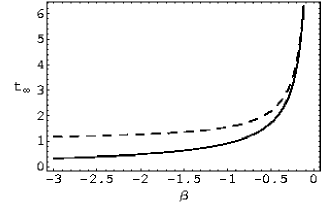
Figure 1: This figure shows the behavior of the cosmic time corresponding to the big rip as a function of the parameter $\beta$ related to the ratio between the pressure and the energy density of the phantom matter. The dashed line corresponds to the case of a FLRW universe sliced into hyperbolic sections. The solid line corresponds to a homogeneous and isotropic space-time sliced into spherical sections. The cosmic time has been divided by $C^{1/(3\beta-2)}$.

Before concluding this section, we will analyze if the inclusion of a constant positive vacuum energy density; i.e. a positive cosmological constant $\Lambda$, may alleviate the big rip problem dues to phantom energy with constant equation of state ($\beta$ constant). For simplicity and analyticity, we will restrict to the case of a FLRW universe with flat spatial geometry. The Friedmann equation reads

$$H^{2}=\frac{\Lambda}{3}+Ca^{-3\beta}.$$ (10)

The solution to the last equation is

$$a^{3\beta}(t) = a_{0}^{3\beta}(1-D)^{-2}\left(\exp\left[\frac{3\beta}{2}\sqrt{\tilde{\Lambda}}(t-t_{0})\right]\right.$$ (11)

$$-\left.D\exp\left[-\frac{3\beta}{2}\sqrt{\tilde{\Lambda}}(t-t_{0}))\right]\right)^{2},$$

where $\tilde{\Lambda}=\Lambda/3$ and $D$ is a positive constant given by

$$D=\frac{\sqrt{\tilde{\Lambda}+Ca_{0}^{-3\beta}}-\sqrt{\tilde{\Lambda}}}{\sqrt{\tilde{\Lambda}+Ca_{0}^{-3\beta}}+\sqrt{\tilde{\Lambda}}}.$$ (12)

From Eq. (11), it can be seen that the scale factor grows from an initial value $a_{0}$ and blows up in a finite cosmic time; i.e. the universe will face a cosmic doomsday, when $t$ approaches $\tilde{t}=t_{0}+(\ln D)/(3\beta\sqrt{\tilde{\Lambda}})$. For $\tilde{t}<t$, the scale factor decreases and the universe collapses when $t$ approaches infinite values. In addition, the larger is the value of $a_{0}$, the smaller is $\tilde{t}$, and consequently, the sooner the cosmic doomsday happens. A similar conclusion holds for $\beta$ (at least for $a_{0}>1$). Moreover, it can be checked that $\tilde{t}$ approaches $t_{\infty 0}$, defined in Eq. (3), when the cosmological constant vanishes. In summary, we have that the presence of a cosmological constant does not modify the general features of the model and the big rip cannot be avoided for $\beta$ constant and negative. Moreover, a positive vacuum energy density cannot delay the happening of the big rip [see Fig. 2]. This can be explained as follows: the presence of a positive cosmological constant in the model induces a bigger growth of the Hubble parameter and, consequently, the scale factor increases faster leading to a sooner big rip.

Figure 2: This figure shows the behavior of the cosmic time corresponding to the big rip as a function of the cosmological constant. As the graphic shows, the largest value for $\tilde{t}$ is achieved in the absence of a positive cosmological constant. Indeed, the larger is $\tilde{\Lambda}$, the sooner the big rip takes place. The cosmological constant and the cosmic time in the graphic are redefined as dimensionless quantities given by $\tilde{\Lambda}/(Ca_{0}^{-3\beta})$ and $-(3/2)\beta\sqrt{C}a_{0}^{-3\beta/2}(\tilde{t}-t_{0})$, respectively.

III Generalized Chaplygin gas and phantom energy

The generalized Chaplygin gas can be described as a perfect fluid with the following equation of state chaplygin

$$P=-A/\rho^{\alpha},$$ (13)

where $A$ is a positive constant and $\alpha$ is a parameter. In the particular case $\alpha=1$, the equation of state (13) corresponds to a Chaplygin gas. The conservation of the energy momentum tensor implies

$$\rho=\left[A+\frac{(\rho_{0}^{\alpha+1}-A)a_{0}^{3(\alpha+1)}}{a^{3(\alpha+1)}}\right]^{\frac{1}{1+\alpha}},$$ (14)

where $a_{0}$ and $\rho_{0}$ are the initial scale factor and energy density, respectively. It can be checked that the dominant energy condition is fulfilled whenever $A<\rho^{(\alpha+1)}$. This requirement is strongly related to the initial values of the model and the specific equation of state through the constant

$$B\equiv(\rho_{0}^{\alpha+1}-A)a_{0}^{3(\alpha+1)}.$$ (15)

For positive values of $B$, $P+\rho$ is positive and the dominant energy condition is satisfied. This is not the case, when $B$ is negative. Let us see the behaviour of the energy density for both cases.

When the parameter $B$ is positive, $\rho$ will be a decreasing function of $a$. In fact, for $1+\alpha>0$ the generalized Chaplygin gas interpolates between dust for small scale factors and a constant energy density at large scale factors. This property has promoted the generalized Chaplygin gas to be a candidate to unify dark energy and dark matter chaplygin . For $1+\alpha<0$, the energy density behaves on the other way round; i.e. $\rho$ approaches $A^{1/(1+\alpha)}$ for small scale factor and behaves as a pressureless fluid at late time.

When the parameter $B$ is negative, the energy density will be an increasing function of the scale factor. Moreover, $\rho$ is larger than $A^{1/(1+\alpha)}$ when $1+\alpha<0$, reaching its minimum value at $a=0$ and blowing up when the scale factor approaches its maximum value

$$\bar{a}\equiv\left(-\frac{B}{A}\right)^{1/[3(1+\alpha)]}.$$ (16)

In what follows, we will disregard this set up ($B<0$ and $1+\alpha<0$). On the other hand, if $1+\alpha>0$ and $B<0$, the scale factor is larger than $\bar{a}$, in such a way that $\rho$ vanishes at this scale factor and approaches $A^{1/(1+\alpha)}$ when the scale factor goes to infinity. We will henceforth analyze this last case, which can be included in the set of phantom energy models as $\rho>0$ and $P+\rho<0$.

As in the previous section, we consider a homogeneous and isotropic universe, where now the phantom energy is given by a generalized Chaplygin gas such that $B<0$ and $-1<\alpha$. The Friedmann equation reads

$$H^{2}+\frac{k}{a^{2}}=\frac{8\pi\textrm{G}}{3}\left[A+\frac{B}{a^{3(\alpha+1)}}\right]^{\frac{1}{1+\alpha}}.$$ (17)

If the FLRW universe is sliced into flat sections, then the cosmic time is related to the scale factor as

$$t-t_{0} = \frac{2D^{-\frac{1}{2}}A^{-\frac{1}{2(1+\alpha)}}}{3(1+2\alpha)}\left[1+\frac{B}{A}a^{-3(1+\alpha)}\right]^{\frac{1+2\alpha}{2(1+\alpha)}}$$

$$\times \textrm{F}\left(1,\frac{1+2\alpha}{2(1+\alpha)};\frac{3+4\alpha}{2(1+\alpha)};1+\frac{B}{A}a^{-3(1+\alpha)}\right),$$

where $D=8\pi G/3$ and $-1/2<\alpha$. Firstly, we have that the scale factor is bigger than $\bar{a}$ defined in Eq. (16). In this case there is no big rip: when the scale factor blows up, the cosmic time does too (see footnote 4). In opposition with the cases studied in the previous section, the present model does not show a cosmic doomsday because the Hubble parameter approaches a constant non vanishing value for large scale factors. Consequently, at late time the geometry of the model is asymptotically de Sitter. Although we have not been able to get an equivalent analytical expression to Eq. (LABEL:agcg) for $-1<\alpha<-1/2$, a similar conclusion holds because $H^{2}$ approaches a positive non vanishing value when $a\rightarrow+\infty$.

When the spatial geometry of the homogeneous and isotropic space-time is spherical, the Hubble parameter is well defined as long as $a>a_{\textrm{min}}$, where $a_{\textrm{min}}$ is such that $H(a_{\textrm{min}})=0$. The explicit expression of $a_{\textrm{min}}$ is given in the appendix. It can be shown that $a_{\textrm{min}}$ is larger than the minimum value of the scale factor for flat spatial geometry given in Eq. (16). Moreover, the cosmic time for $k=1$ satisfies the inequality

$$t-t_{0} > \int_{\bar{a}}^{a}\left[Da^{2}\left(A+\frac{B}{a^{3(1+\alpha)}}\right)^{\frac{1}{1+\alpha}}\right]^{-\frac{1}{2}}da$$

$$- \int_{\bar{a}}^{a_{\textrm{min}}}\left[Da^{2}\left(A+\frac{B}{a^{3(1+\alpha)}}\right)^{\frac{1}{1+\alpha}}\right]^{-\frac{1}{2}}da.$$

The second term on the right hand side (rhs) of the inequality is finite. Indeed, it is the cosmic time for flat spatial sections corresponding to $a=a_{\textrm{min}}$. In addition, the first term on the rhs corresponds to the cosmic time for $k=0$ geometry at a given scale factor $a>\bar{a}$. As can be seen for large scale factor the cosmic time for $k=1$ blows up because $t-t_{0}$ diverges for flat spatial geometry (first term on rhs). Consequently, the universe does not hit a cosmic doomsday in its future.

Similarly, the cosmic time for a FLRW universe with spatial hyperbolic sections can be bounded from below as follows

$$t-t_{0} > \frac{1}{\sqrt{2}}\Big{\{}a_{\textrm{min}}-\bar{a}\Big{.}$$

$$+ \Big{.}\int_{\bar{a}}^{a}\left[Da^{2}\left(A+\frac{B}{a^{3(1+\alpha)}}\right)^{\frac{1}{1+\alpha}}\right]^{-\frac{1}{2}}da\Big{.}$$

$$- \Big{.}\int_{\bar{a}}^{a_{\textrm{min}}}\left[Da^{2}\left(A+\frac{B}{a^{3(1+\alpha)}}\right)^{\frac{1}{1+\alpha}}\right]^{-\frac{1}{2}}da\Big{\}},$$

when the matter content corresponds to a generalized Chaplygin gas. We would like to point out that the last two terms on rhs of the inequality coincides precisely with the ones on the rhs of the expression (LABEL:inequality+1). Consequently, based on an argument similar to that is used for the $k=1$ case, we can conclude that there is no big rip for $k=-1$. In addition, the scale factor grows from $\bar{a}$ to infinity.

Once analyzed the late time behaviour of a homogeneous and isotropic space-time filled by a generalized Chaplygin gas with the characteristics already mentioned, let us see how it behaves for smaller scale factors. The energy density vanishes whenever the scale factor approaches $\bar{a}$, which can be the case only for flat and hyperbolic sections. Consequently, at $a=\bar{a}$ the pressure may diverge inducing a singularity in the geometry [see Fig. 3]. Indeed this can be the case if $\alpha$ is positive. The scalar curvature for $k=\pm 1,0$ reads

$$R = 6\left(\dot{H}+2H^{2}+\frac{k}{a^{2}}\right)$$

$$= 12D\left[A+\frac{B}{4a^{3(1+\alpha)}}\right]\left[A+\frac{B}{a^{3(1+\alpha)}}\right]^{-\frac{\alpha}{1+\alpha}},$$

where the dot represents derivative respect to the cosmic time. As can be seen, $R$ is well defined at any scale factor for spherical geometry (we recall $\bar{a}<a_{\textrm{min}}$). On the other hand, for $k=-1,0$, the scalar curvature $R$ is finite (even at $a=\bar{a}$) as long as $-1<\alpha<0$. The same can de deduced for positive values of $\alpha$ except at $a=\bar{a}$, where there is a divergence of $R$. We would like also to point out that for flat sections the FLRW universe presents a bouncing at $a=\bar{a}$, which is regular if $-1<\alpha<0$.

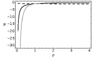
Figure 3: The behavior of the pressure of the generalized Chaplygin gas is shown in terms of its energy density for negative values of the parameter $B$. The dashed line corresponds to $\alpha=-0.1$. The solid darkest (lightest) line corresponds to $\alpha=1$ ($\alpha=2$). The pressure and energy density has been redefined as dimensionless quantities given by $PA^{-1/(1+\alpha)}$ and $\rho A^{-1/(1+\alpha)}$, respectively. As can be seen, for positive values of $\alpha$ the pressure reaches extremely negative value when $\rho$ approaches zero.

Before concluding this section, we analyze the parameter $\beta(a)=P/\rho+1$, which somehow quantifies the deviation of the generalized Chaplygin gas from a cosmological constant [see Fig. 4] and can be expressed in terms of the scale factor as

$$\beta=\frac{B}{B+Aa^{3(1+\alpha)}}.$$ (22)

As can be expected $\beta$ is negative for the set of parameters we are considering. At late time, $\beta$ approaches zero; i.e. the FLRW universe is asymptotically de Sitter. On the other hand, $\beta$ blows up near $\bar{a}$ (only for $k=0,-1$). This is partially due to our oversimplified model. In principle, we should have considered the other matter contents of the universe, as dark matter component, which are the dominant components for smaller scale factors. Indeed, if we consider dark matter (DM) given by dust, the effective value of $\beta$ approaches the unity; i.e. the total matter content behaves effectively as dust, when $a\rightarrow\bar{a}$, as long as $-1<\alpha<0$. For positive value of $\alpha$ the effective value of $\beta$ is still divergent at $\bar{a}$. This can be understood as a consequence of the divergence of $P$ near $\bar{a}$ for positive $\alpha$.

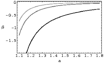
Figure 4: This plot shows the behavior of the parameter $\beta$ given in Eq. (22) as a function of the dimensionless variable $a/\bar{a}$. The lower graphic (the darkest one) corresponds to $\alpha=-0.1$. The upper graphic (the lightest one) corresponds to $\alpha=2$. Finally, the middle graphic shows $\beta$ for the Chaplygin gas; i.e. $\alpha=1$. As can be see, the generalized Chaplygin gas approaches a positive cosmological constant ($\beta=0$) for the largest values of the scale factor.

In summary, we have shown that a generalized Chaplygin gas can describe phantom energy. In addition, this material content can avoid the occurrence of a cosmic doomsday in the future of the universe. This is not surprising as the energy density of a generalized Chaplygin gas approaches a constant positive value for $B<0$ and $0<\alpha+1$. Consequently, a FLRW universe filled with this gas is asymptotically de Sitter.

IV Generalized Chaplygin gas and scalar fields

Up to now, we have described the generalized Chaplygin as a perfect fluid with a peculiar equation of state (13). In the following, we will describe the generalized Chaplygin gas in terms of scalar fields. First, we will show how the generalized Chaplygin gas (with a negative parameter $B$, see Eq. (15)) can emerge in the context of generalized Born-Infeld phantom theories. For this purpose, we consider the Lagrangian $\mathcal{L}_{\phi}$ defined as

$$\mathcal{L}_{\phi}=-A^{\frac{1}{1+\alpha}}\left[1+\left(-g^{\mu\nu}\nabla_{\mu}\phi\nabla_{\nu}\phi\right)^{\frac{1+\alpha}{2\alpha}}\right]^{\frac{\alpha}{1+\alpha}},$$ (23)

where $g_{\mu\nu}$ is the metric of the space-time and $\phi$ is a scalar field. For a FLRW universe, $\mathcal{L_{\phi}}$ reduces to

$$\mathcal{L}_{\phi}=-A^{\frac{1}{1+\alpha}}\left[1+(\dot{\phi})^{\frac{1+\alpha}{\alpha}}\right]^{\frac{\alpha}{1+\alpha}}.$$ (24)

The dot corresponds to derivative respect to the cosmic time. It can be shown that the energy density $\rho_{\phi}$ and the pressure $P_{\phi}$ associated to $\mathcal{L_{\phi}}$ reads Armendariz-Picon:1999rj ,

$$\rho_{\phi} = A^{\frac{1}{1+\alpha}}\left[1+(\dot{\phi})^{\frac{1+\alpha}{\alpha}}\right]^{-\frac{1}{1+\alpha}},$$

$$P_{\phi} = -A^{\frac{1}{1+\alpha}}\left[1+(\dot{\phi})^{\frac{1+\alpha}{\alpha}}\right]^{\frac{\alpha}{1+\alpha}},$$ (25)

Consequently, $\rho_{\phi}$ and $P_{\phi}$ satisfy a generalized Chaplygin gas equation of state; i.e. $P_{\phi}=-A/\rho_{\phi}^{\alpha}$. The difference between the Lagrangian defined by expression (23) and the one given in chaplygin is that the kinetic energy term for the scalar field $\phi$ is negative. In addition, it can be seen that

$$P_{\phi}/\rho_{\phi}=-[1+(\dot{\phi})^{\frac{1+\alpha}{\alpha}}].$$ (26)

This expression shows that the scalar field $\phi$ behaves as phantom energy [see also Eq. (27)]. Moreover, this characteristic of $\phi$ allows negative values of the parameter $B$, defined in Eq. (15), as has been considered in the last section. Additionally, on the one hand, the time derivative of $\phi$ scales with the scale factor as

$$\dot{\phi}^{\frac{1+\alpha}{\alpha}}=\frac{-B}{B+Aa^{3(1+\alpha)}}.$$ (27)

On the other hand, for FLRW universes with flat or hyperbolic spatial sections filled by a generalized Chaplygin gas with $B<0$ and $-1<\alpha$, the scale factor can takes any value such that $\bar{a}\leq a$ ($\bar{a}$ is defined in Eq. (16)). Consequently, for $-1<\alpha<0$, $\dot{\phi}$ vanishes when $a$ approaches $\bar{a}$. However, for positive values of $\alpha$, the time derivative of $\phi$ diverges when $a$ approaches $\bar{a}$. For large value of the scale factor the opposite behavior is found; i.e. $\dot{\phi}$ approaches zero when $0<\alpha$ and diverges when $-1<\alpha<0$. The divergence of $\dot{\phi}$ is harmless for large values of the scale factor, as the geometry of the universe behaves like a de Sitter space-time and, consequently, there is no singularity. Additionally, in a FLRW universe with a flat spatial geometry the scalar field $\phi$ varies with the scale factor as

$$\phi-\phi_{0}=\frac{A^{-\frac{1}{2(1+\alpha)}}}{\sqrt{6\pi G}}\left[1-\left(\frac{\bar{a}}{a}\right)^{3(1+\alpha)}\right]^{\frac{1}{2(1+\alpha)}}$$

$$\times \textrm{F}\left(\frac{1}{1+\alpha},\frac{1}{2(1+\alpha)};\frac{1}{2(1+\alpha)}+1;1-\left(\frac{\bar{a}}{a}\right)^{3(1+\alpha)}\right),$$

where $-1<\alpha$ and $\phi_{0}$ is an integration constant corresponding to the value acquired by $\phi$ at $a=\bar{a}$. The scalar field $\phi$ is finite for any value of the scale factor, whenever $\alpha$ is positive (see footnote 4). For $-1<\alpha<0$, the last affirmation remains true except for very large values of the scale factor, where $\phi$ blows up (see Fig. 5).

Figure 5: This figure shows the behavior of the scalar field $\phi$ as a function of the dimensionless scale factor $a/\bar{a}$ given in Eq. (LABEL:phi). The graphic with dashed line corresponds to $\alpha=-0.1$, while the graphic with darkest (lightest) full line corresponds to $\alpha=1$ ($\alpha=2$). In the plot, the scalar field $\phi$ has been redefined as $\sqrt{6\pi\textrm{G}}A^{{1}/(2(1+\alpha))}(\phi-\phi_{0})$.

In the following, we show how the generalized Chaplygin gas can be described effectively in terms of a Born-Infeld phantom scalar field, $\psi$, whose Lagrangian reads

$$\mathcal{L}_{\psi}=-V(\psi)\sqrt{1-g^{\mu\nu}\nabla_{\mu}\psi\nabla_{\nu}\psi}.$$ (29)

For a homogenous and isotropic space-time, the energy density $\rho_{\psi}$ and the pressure $P_{\psi}$ associated to $\psi$ reads Li ; Armendariz-Picon:1999rj

$$\rho_{\psi}=\frac{V(\psi)}{\sqrt{1+\dot{\psi}^{2}}},\quad P_{\psi}=-V(\psi)\sqrt{1+\dot{\psi}^{2}}.$$ (30)

Obviously, for a Chaplygin gas; i.e. $\alpha=1$, with phantom energy characteristics, the potential $V(\psi)$ is constant; $V=\sqrt{A}$ (see Eq. (23) for $\alpha=1$). However, in general a generalized Chaplygin gas can be described effectively by a Born-Infeld phantom scalar field, $\psi$, only when its potential depends explicitly on $\psi$. In fact, it can be easily seen that $V$ varies with the scale factor as follows

$$V(a)=\sqrt{A}\left(A+\frac{B}{a^{3(1+\alpha)}}\right)^{\frac{1-\alpha}{2(1+\alpha)}}.$$ (31)

The potential $V$ approaches a constant value for large values of the scale factor (we are considering $-1<\alpha$ and $B<0$). In addition, its behaviour near the minimum value of the scale factor, $\bar{a}$, (for $k=0,-1$), depends strongly on the specific value of the parameter $\alpha$: for $|\alpha|<1$ the potential vanishes near $\bar{a}$, for $1<|\alpha|$ the potential blows up (see Fig. 6). A main difference between the behaviour of the scalar fields $\psi$ and $\phi$ is that $\dot{\psi}$ always reaches large values near $\bar{a}$, while this is not necessarily true for $\dot{\phi}$. Additionally, it can be seen that for a FLRW universe with spatially flat sections, the scalar field $\psi$ varies with the scale factor as

$$\psi - \psi_{0}=\frac{A^{-\frac{1}{2(1+\alpha)}}}{\sqrt{6\pi G}\alpha}\left[1-\left(\frac{\bar{a}}{a}\right)^{3(1+\alpha)}\right]^{\frac{\alpha}{2(1+\alpha)}}$$

$$\times \textrm{F}\left(\frac{1}{2},\frac{\alpha}{2(1+\alpha)};\frac{\alpha}{2(1+\alpha)}+1;1-\left(\frac{\bar{a}}{a}\right)^{3(1+\alpha)}\right),$$

when $\alpha$ is positive. In the last equation $\psi_{0}$ is a constant corresponding to the value acquired by $\psi$ at $a=\bar{a}$. It can be shown that $\psi$ is finite for any value of the scale factor (see footnote 4). On the other hand, for $-1<\alpha<0$, the scalar field scales with $a$ as

$$\psi-\psi_{\infty} = \frac{A^{-\frac{1}{2(1+\alpha)}}}{\sqrt{6\pi G}(1+\alpha)}\left(\frac{\bar{a}}{a}\right)^{\frac{3(1+\alpha)}{2}}$$ (33)

$$\times \textrm{F}\left(\frac{2+\alpha}{2(1+\alpha)},\frac{1}{2};\frac{3}{2};\left(\frac{\bar{a}}{a}\right)^{3(1+\alpha)}\right),\,\,$$

where $\psi_{\infty}$ is the value reached by $\psi$ for very large scale factors. In this case, the scalar field $\psi$ is well behaved for any value of $a$, expect at $a=\bar{a}$ where it blows up.

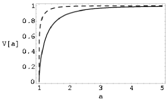
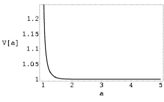
Figure 6: These figures show the behavior of $V(a)$ defined in Eq. (31) as a function of the scale factor. The figure on the top corresponds to the values $\alpha=-0.1$ (full line) and $\alpha=1/2$ (dashed line). The figure on the bottom corresponds to $\alpha=2$. The potential $V(a)$ has been redefined as $A^{-{1}/(1+\alpha)}V(a)$ and the scale factor as $a/\bar{a}$.

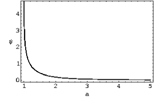
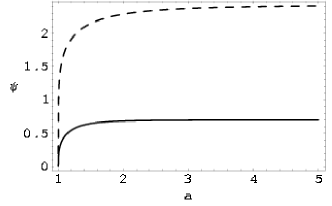
Figure 7: These figures show the behavior of $\psi$ defined in Eqs. (LABEL:psi1) and (33) as a function of the scale factor for a FLRW universe with flat spatial sections. The figure on the top corresponds to $\alpha=-0.1$. The figure on the bottom corresponds to $\alpha=0.5$ (dashed line) and $\alpha=2$ (full line). In the top plot, the scalar field $\psi$ has been redefined as $\sqrt{6\pi\textrm{G}}A^{{1}/(2(1+\alpha))}(\psi-\psi_{0})$. In the bottom plot $\psi$ is redefined as $\sqrt{6\pi\textrm{G}}A^{{1}/(2(1+\alpha))}(\psi-{\psi}_{\infty})$. In both plots the scale factor has been divided by $\bar{a}$.

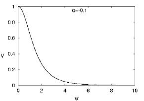
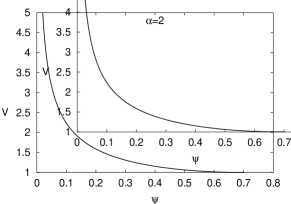
Figure 8: These figures show the behavior of $V$ as a function of the scalar field $\psi$ [see Eqs. (31), (LABEL:psi1)and (33)] for a FLRW universe with flat spatial sections. The figures starting from the top correspond to $\alpha=-0.1$, $\alpha=0.5$ and $\alpha=2$, respectively. The potential $V$ has been redefined as $A^{-{1}/(1+\alpha)}V$. In the top plot $\psi$ is redefined as $\sqrt{6\pi\textrm{G}}A^{{1}/(2(1+\alpha))}(\psi-{\psi}_{\infty})$. On the other plots, the scalar field $\psi$ has been redefined as $\sqrt{6\pi\textrm{G}}A^{{1}/(2(1+\alpha))}(\psi-\psi_{0})$.

Finally, we analyze the behaviour of a phantom minimally coupled scalar field, $\chi$, able to mimic the behaviour of a generalized Chaplygin gas (for $B$ negative and $-1<\alpha$). In this case, the energy density $\rho_{\chi}$ and pressure $P_{\chi}$ of the homogeneous scalar field $\chi$ read

$$\rho_{\chi}=-\frac{1}{2}{\dot{\chi}}^{2}+\tilde{V}(\chi),\quad P_{\chi}=-\frac{1}{2}{\dot{\chi}}^{2}-\tilde{V}(\chi).$$ (34)

If the scalar field $\chi$ simulates a generalized Chaplygin gas, the potential $\tilde{V}$ scales with the scale factor as

$$\tilde{V}(a)=\frac{1}{2}\left[A+\frac{B}{a^{3(1+\alpha)}}\right]^{-\frac{\alpha}{1+\alpha}}\left[2A+\frac{B}{a^{3(1+\alpha)}}\right].$$ (35)

As can be seen, $\tilde{V}(a)$ approaches a constant value when $a$ blows up. This is not surprising: as we have already mentioned a FLRW universe filled with a generalized Chaplygin gas is asymptotically de Sitter. For the scalar field, $\chi$, this results on $\tilde{V}(a)$ approaching a non vanishing constant and a vanishing $\dot{\chi}$ for very large scale factors. In addition, $\tilde{V}(a)$ is finite when $a$ approaches $\bar{a}$ (for $k=0,-1$) as long as $-1<\alpha<0$. However, for positive values of $\alpha$, the potential $\tilde{V}$ blows up near $\bar{a}$. Moreover, If the FLRW universe is spatially flat, $\chi$ is well behaved for any value of $a$. In fact, its evolution can be described in term of the scale factor as

$$\chi-\chi_{0} = \frac{1}{(1+\alpha)\sqrt{24\pi\textrm{G}}}$$ (36)

$$\times \left\{\frac{\pi}{2}-\arcsin\left[2\left(\frac{\bar{a}}{a}\right)^{3(1+\alpha)}-1\right]\right\},$$

where $\chi_{0}$ is an integration constant. In a addition, the potential $\tilde{V}$ varies with $\chi$ as

$$\tilde{V}(\chi) = \frac{1}{2}\left(\frac{A}{2}\right)^{\frac{1}{1+\alpha}}$$

$$\times \frac{3-\cos\left[(1+\alpha)\sqrt{24\pi\textrm{G}}(\chi-\chi_{0})\right]}{\left\{1-\cos\left[(1+\alpha)\sqrt{24\pi\textrm{G}}(\chi-\chi_{0})\right]\right\}^{\frac{\alpha}{1+\alpha}}}.$$

The behaviour of the potential $\tilde{V}(\chi)$ depends strongly on the value of the parameter $\alpha$ (see Fig. 9).

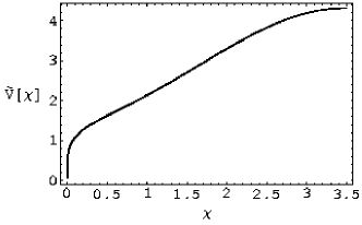
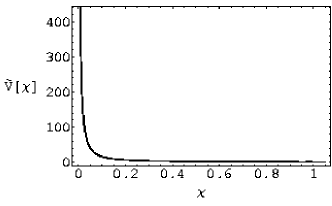
Figure 9: These figures show the behaviour of $\tilde{V}(\chi)$ defined in Eq. (LABEL:Vchi) as a function of the minimally coupled scaler field $\chi$ for a FLRW universe with flat spatial sections. The figure on the top corresponds to $\alpha=-0.1$. The figure on the bottom corresponds to $\alpha=2$. In the plots, the scalar field $\chi$ has been redefined as $\sqrt{24\pi\textrm{G}}(\chi-\chi_{0})$ and the potential as $2(2/A)^{1/(1+\alpha)}\tilde{V}(\chi)$. As can be seen the behaviour of $\tilde{V}$ depends on the chosen value of $\alpha$. For negative values of $\alpha$ the scalar field rolls up the potential. However, for positive values of $\alpha$, the scalar field $\chi$ rolls down the potential.

For $-1<\alpha<0$ the scalar field rolls up the potential. However, for positive values of $\alpha$, the scalar field $\chi$ rolls down the potential in contrast with the result obtained in Ref. SSD . In the first case, the scalar field starts with a vanishing velocity ($\dot{\chi}=0$) climbing the potential. Its velocity continues increasing until it reaches a maximum value and then it starts decreasing, vanishing for very large values of the scale factor (see Fig. 10). In the second case, $\chi$ starts with an infinite velocity rolling down the potential. Its velocity is continuously decreasing, until vanishing when the scale factor blows up (see Fig. 10).

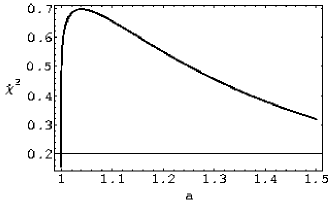
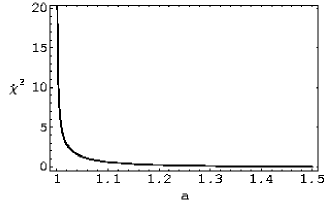
Figure 10: The behaviour of the quadratic velocity of the scalar field $\dot{\chi}^{2}$ is shown as a function of $a/\bar{a}$. The figure on the top corresponds to $\alpha=-0.1$, while the figure on the bottom corresponds to $\alpha=2$. $\dot{\chi}^{2}$ has been redefined as $A^{-1/(1+\alpha)}\dot{\chi}^{2}$.

V A phenomenologically viable model

In order to study the possible occurrence of a big rip (in the future of the universe) caused by phantom energy, it is a good approximation to consider that the matter content of the universe is mainly given by phantom energy at very late time (large scale factors). However, any cosmological viable model able to describe the actual acceleration of the universe has to take into account the other material components of the universe, in particular DE. Consequently, the Friedmann equation reads

$$H^{2}=\frac{8\pi\textrm{G}}{3}\left(\rho_{\textrm{DE}}+\rho_{\textrm{DM}}+\rho_{\textrm{R}}\right),$$ (38)

where $\rho_{\textrm{DE}},\rho_{\textrm{DM}},\rho_{\textrm{R}}$ correspond, respectively, to the energy density of DE, DM, and radiation. We will consider that DE is described by a generalized Chaplygin gas with $B<0$ and $-1<\alpha$ (see Eq. (14)) and the DM component as a dust fluid. The Friedmann equation can be rewritten as

$$H^{2}=H_{i}^{2}\left[\frac{\rho_{\textrm{DE}}}{\rho_{C,i}}+\Omega_{\textrm{DM}}\left(\frac{a_{i}}{a}\right)^{3}+\Omega_{\textrm{R}}\left(\frac{a_{i}}{a}\right)^{4}\right].$$ (39)

In the last expression, $H_{i},a_{i},\rho_{C,i}$ are the present Hubble parameter, scale factor and critical energy density. On the other hand, $\Omega_{\textrm{DM}}$ and $\Omega_{\textrm{R}}$ are the density parameters for DM and radiation. The model can describe the present acceleration of the universe as long as ${\rho_{\textrm{DE}}}/{\rho_{C,i}}\simeq 0.7$, $\Omega_{\textrm{R}}\simeq 0.3$ and $\Omega_{\textrm{R}}\simeq 0$. On the other hand, at the radiation dominated era ($T=1MeV$) the energy density must be dominated by the $\rho_{\textrm{R}}$ (for a successful Nucleosynthesis). Considering that the present scale factor is equal to the unity, the scale factor in the radiation dominated era is equal to $2.4\times 10^{-10}$. Our model can describe a viable cosmological model satisfying all these requirements for different values of $\alpha$ [see Fig. 11], although there is a fine tuning of the parameters $A$ and $B$.

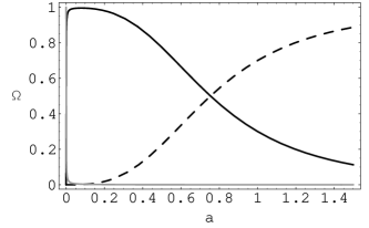
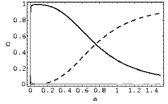
Figure 11: These figures shows the behavior of $\Omega_{\textrm{DE}}$, $\Omega_{\textrm{DM}}$ and $\Omega_{R}$ as a function of the scale factor since the nucleosynthesis epoch; i.e. $\rho_{r}=1MeV$ . The lightest graphics correspond to $\Omega_{R}$. The darkest full line graphics correspond to $\Omega_{\textrm{DM}}$. Finally, the dashed line graphics correspond to $\Omega_{\textrm{DE}}$. On the one hand, in the figure of the top, it has been chosen $\alpha=-0.1$, $A^{1/(1+\alpha)}\simeq 2.8\times 10^{-11}eV$ and $|B|^{1/(1+\alpha)}\simeq 3.8\times 10^{-40}eV$. On the other hand, on the figure of the bottom, it has been chosen $\alpha=-0.9$, $A^{1/(1+\alpha)}\simeq 2.8\times 10^{-10}eV$ and $|B|^{1/(1+\alpha)}\simeq 1.4\times 10^{-41}eV$. As can be seen the behavior is very similar for both choices.

VI Conclusions

In this paper we study the behaviour of several phantom energy models able to describe effectively dark energy. First, we review the dynamics of a FLRW universe with phantom energy given by a perfect fluid with a constant equation of state; i.e. $P=(\beta-1)\rho$ where $\beta$ is constant and negative. It is shown that the universe hits a big rip independently of the spatial geometry of the universe. Additionally, it is shown in this setup that the presence of a positive constant energy density in the universe cannot avoid the happening of a cosmic doomsday. Indeed, the universe hits the big rip sooner than it would be with $\Lambda=0$.

Secondly, we model dark energy by a phantom generalized Chaplygin gas; i.e. $P=-A/\rho^{\alpha}$. It is shown that this gas behaves as a phantom energy as long as the parameter $B$ is negative [see Eq. (15)]. In addition, the energy density of the gas increases with the expansion of the universe, vanishing for a minimum scale factor and approaching a constant value at very late times (for $-1<\alpha$). Consequently, it can be shown in this case that the universe will never hit a big rip. In fact, the universe is asymptotically de Sitter in this case.

The model involving the phantom generalized Chaplygin gas can describe the actual acceleration of the universe [see Sec. V], where the energy density of the gas corresponds roughly to two thirds of the total energy density of the universe. However, there is a fine tuning between the parameters $A$ and $B$ related to the energy density of the gas.

We have also shown how the phantom generalized Chaplygin gas can appear in a natural way in the context of phantom generalized Born-Infeld theories, where the kinetic energy term for the scalar field is negative. In addition, we have analyzed different effective phantom scalar fields which can mimic the behaviour of this gas. This has been carried out in the context of a Born-Infeld scalar field and a minimally coupled scalar field. Although, the dynamics of each of this scalar fields can be quite different, they provide the same behaviour for the scale factor and avoid the occurrence of a cosmic doomsday in the future of the universe.

Finally, we would like to stress that a phantom energy model does not necessarily imply a big rip in the future of the universe as has been shown using a phantom generalized Chaplygin gas, even without imposing any restriction on the sound speed phantom2 . Moreover, a big rip singularity is not necessarily related to a phantom matter content as has been recently pointed out in Barrow:2004xh . Although there the big rip singularity happens in a finite cosmic time, scale factor, energy density and Hubble constant; and the singularity is associated with a divergence of the pressure.

Appendix A Explicit expression of $\mathbf{a_{\textrm{min}}}$

The Friedmann equation (17) for $k=1$ can be expressed as $H^{2}=f(a)$ where

$$f(a)=-1/a^{2}+D\left[A+\frac{B}{a^{3(1+\alpha)}}\right]^{\frac{1}{1+\alpha}}.$$ (40)

The function $f(a)$ has a unique positive root which we have denoted $a_{\textrm{min}}$. Its corresponds to the minimum radius of a FLRW universe filled by a generalized Chaplygin gas with $B$ negative and $-1<\alpha$. The explicit expression of $a_{\textrm{min}}$ depends on the parameter X

$$Q\equiv\frac{B^{2}}{4A^{2}}-\frac{D^{-3(1+\alpha)}}{27A^{3}}.$$ (41)

For positive value of $Q$; i.e. $(27/4)D^{3(1+\alpha)}AB^{2}>0$, $a_{\textrm{min}}$ reads

$$a_{\textrm{min}}=\left[\left(-\frac{B}{2A}+\sqrt{Q}\right)^{\frac{1}{3}}+\left(-\frac{B}{2A}-\sqrt{Q}\right)^{\frac{1}{3}}\right]^{\frac{1}{1+\alpha}}.$$ (42)

For $Q=0$ that is $B^{2}=4/(27D^{3(1+\alpha)}A)$, $a_{\textrm{min}}$ is

$$a_{\textrm{min}}=\frac{1}{\sqrt{D}}\left(\frac{4}{3A}\right)^{\frac{1}{2(1+\alpha)}}.$$ (43)

Finally, if $(27/4)D^{3(1+\alpha)}AB^{2}<0$; i.e. negative value of $Q$, $a_{\textrm{min}}$ can be expressed as

$$a_{\textrm{min}}=\left[2\varrho^{1/3}\cos\left(\frac{\theta}{3}\right)\right]^{\frac{1}{1+\alpha}},$$ (44)

where

$$\varrho = \frac{1}{\sqrt{27D^{3(1+\alpha)}A^{3}}},$$

$$\theta = \arctan\sqrt{-1+\frac{4}{27D^{3(1+\alpha)}AB^{2}}}.$$ (45)

It can be checked that for any value of $Q$, $a_{\textrm{min}}$ is larger than $\bar{a}$ given in Eq. (16).

References

- (1) D. N. Spergel et al., Astrophys. J. Suppl. 148, 175 (2003) [arXiv:astro-ph/0302209]; C. L. Bennett et al., Astrophys. J. Suppl. 148, 1 (2003) [arXiv:astro-ph/0302207]; M. Tegmark et al. [SDSS Collaboration], arXiv:astro-ph/0310723.
- (2) A. G. Riess et al. [Supernova Search Team Collaboration], Astron. J. 116, 1009 (1998) [arXiv:astro-ph/9805201]; S. Perlmutter et al. [Supernova Cosmology Project Collaboration], Astrophys. J. 517, 565 (1999) [arXiv:astro-ph/9812133]; J. L. Tonry et al., Astrophys. J. 594, 1 (2003) [arXiv:astro-ph/0305008].
- (3) R. Jimenez, New Astron. Rev. 47, 761 (2003) [arXiv:astro-ph/0305368].
- (4) S. Weinberg, Rev. Mod. Phys. 61, 1 (1989); P. J. E. Peebles and B. Ratra, Rev. Mod. Phys. 75, 559 (2003) [arXiv:astro-ph/0207347]; T. Padmanabhan, Phys. Rept. 380, 235 (2003) [arXiv:hep-th/0212290].
- (5) A. Y. Kamenshchik, U. Moschella and V. Pasquier, Phys. Lett. B 511, 265 (2001) [arXiv:gr-qc/0103004]; V. Gorini, A. Kamenshchik and U. Moschella, Phys. Rev. D 67, 063509 (2003) [arXiv:astro-ph/0209395]; N. Bilic, G. B. Tupper and R. D. Viollier, Phys. Lett. B 535, 17 (2002) [arXiv:astro-ph/0111325]; arXiv:astro-ph/0207423; M. C. Bento, O. Bertolami and A. A. Sen, Phys. Rev. D 66, 043507 (2002) [arXiv:gr-qc/0202064]; Phys. Rev. D 67, 063003 (2003) [arXiv:astro-ph/0210468]; Phys. Lett. B 575, 172 (2003) [arXiv:astro-ph/0303538]; O. Bertolami, A. A. Sen, S. Sen and P. T. Silva, arXiv:astro-ph/0402387; V. Gorini, A. Kamenshchik, U. Moschella and V. Pasquier, gr-qc/0403062; O. Bertolami, astro-ph/0403310.
- (6) L. Amendola, F. Finelli, C. Burigana and D. Carturan, JCAP 0307, 005 (2003) [arXiv:astro-ph/0304325]; R. Bean and O. Dore, Phys. Rev. D 68, 023515 (2003) [arXiv:astro-ph/0301308]; J. C. Fabris, S. V. Goncalves and P. E. de Souza, Gen. Rel. Grav. 34, 53 (2002) [arXiv:gr-qc/0103083]; Gen. Rel. Grav. 34, 2111 (2002) [arXiv:astro-ph/0203441]; R. Colistete, J. C. Fabris, S. V. Goncalves and P. E. de Souza, arXiv:gr-qc/0210079; H. Sandvik, M. Tegmark, M. Zaldarriaga and I. Waga, arXiv:astro-ph/0212114; L. M. Beca, P. P. Avelino, J. P. de Carvalho and C. J. Martins, Phys. Rev. D 67, (2003) 101301 [arXiv:astro-ph/0303564]; T. Multamaki, M. Manera and E. Gaztanaga, Phys. Rev. D 69, 023004 (2004) [arXiv:astro-ph/0307533]; A. Dev, D. Jain and J.S. Alcaniz, astro-ph/0311056; M. Biesiada, W. Godlowski and M. Szydlowski, astro-ph/0403305.
- (7) M. Bouhmadi-López and P. Vargas Moniz, [arXiv:gr-qc/0404111]
- (8) C. Wetterich, Nucl. Phys. B 302, 668 (1988); B. Ratra and P. J. Peebles, Phys. Rev. D 37, 3406 (1988); R. R. Caldwell, R. Dave and P. J. Steinhardt, Phys. Rev. Lett. 80, 1582 (1998) [arXiv:astro-ph/9708069]; P. F. González-Díaz, Phys. Rev. D 62, 023513 (2000) [arXiv:astro-ph/0004125]; Y. Fujii, Phys. Rev. D 62 064004 (2000) [arXiv:gr-qc/9908021].
- (9) R. R. Caldwell, Phys. Lett. B 545, 23 (2002) [arXiv:astro-ph/9908168].
- (10) R. R. Caldwell, M. Kamionkowski and N. N. Weinberg, Phys. Rev. Lett. 91, 071301 (2003) [arXiv:astro-ph/0302506].
- (11) B. McInnes, JHEP 0208, 029 (2002) [arXiv:hep-th/0112066]; S. M. Carroll, M. Hoffman and M. Trodden, Phys. Rev. D 68, 023509 (2003) [arXiv:astro-ph/0301273].
- (12) P. Singh, M. Sami and N. Dadhich, Phys. Rev. D 68, 023522 (2003) [arXiv:hep-th/0305110]; J. G. Hao and X. z. Li, arXiv:astro-ph/0309746.
- (13) J. g. Hao and X. z. Li, Phys. Rev. D 68, 043501 (2003) [arXiv:hep-th/0305207]; J. g. Hao and X. z. Li, Phys. Rev. D 68, 083514 (2003) [arXiv:hep-th/0306033]; D. j. Liu and X. z. Li, Phys. Rev. D 68, 067301 (2003) [arXiv:hep-th/0307239].
- (14) P. F. González-Díaz, Phys. Rev. D 68, 021303 (2003) [arXiv:astro-ph/0305559]; G. W. Gibbons, arXiv:hep-th/0302199; R. Kallosh, J. Kratochvil, A. Linde, E. V. Linder and M. Shmakova, JCAP 0310, 015 (2003) [arXiv:astro-ph/0307185]; L. P. Chimento and R. Lazkoz, Phys. Rev. Lett. 91, 211301 (2003) [arXiv:gr-qc/0307111]; M. P. Dabrowski, T. Stachowiak and M. Szydlowski, Phys. Rev. D 68, 103519 (2003) [arXiv:hep-th/0307128]; V. Faraoni, Phys. Rev. D 68, 063508 (2003); V. Faraoni, arXiv:gr-qc/0307086; H. Stefancic, arXiv:astro-ph/0310904; V. B. Johri, arXiv:astro-ph/0311293; J. M. Cline, S. y. Jeon and G. D. Moore, arXiv:hep-ph/0311312; H. Q. Lu, arXiv:hep-th/0312082; X. H. Meng and P. Wang, arXiv:hep-ph/0311070; S. Nojiri and S. D. Odintsov, Phys. Lett. B 571, 1 (2003) [arXiv:hep-th/0306212]; S. Nojiri and S. D. Odintsov, Phys. Lett. B 562, 147 (2003) [arXiv:hep-th/0303117]; S. Nojiri and S. D. Odintsov, Phys. Lett. B 565 (2003) 1 [arXiv:hep-th/0304131].
- (15) C. Deffayet, Phys. Lett. B 502, 199 (2001) [arXiv:hep-th/0010186]; C. Deffayet, G. R. Dvali and G. Gabadadze, Phys. Rev. D 65, 044023 (2002) [arXiv:astro-ph/0105068]; V. Sahni and Y. Shtanov, JCAP 0311, 014 (2003) [arXiv:astro-ph/0202346].
- (16) S. M. Carroll, V. Duvvuri, M. Trodden and M. S. Turner, arXiv:astro-ph/0306438.
- (17) G. Ellis and S.W. Hawking, The large scale structure of space-time (Cambridge University Press, 1973).
- (18) C. Armendariz-Picon, T. Damour and V. Mukhanov, Phys. Lett. B 458, 209 (1999) [arXiv:hep-th/9904075]; J. Garriga and V. F. Mukhanov, Phys. Lett. B 458, 219 (1999) [arXiv:hep-th/9904176]; T. Chiba, T. Okabe and M. Yamaguchi, Phys. Rev. D 62, 023511 (2000) [arXiv:astro-ph/9912463]; C. Armendariz-Picon, V. Mukhanov and P. J. Steinhardt, Phys. Rev. Lett. 85, 4438 (2000) [arXiv:astro-ph/0004134]; C. Armendariz-Picon, V. Mukhanov and P. J. Steinhardt, Phys. Rev. D 63, 103510 (2001) [arXiv:astro-ph/0006373]; M. Malquarti, E. J. Copeland, A. R. Liddle and M. Trodden, Phys. Rev. D 67, 123503 (2003) [arXiv:astro-ph/0302279]; M. Malquarti, E. J. Copeland and A. R. Liddle, Phys. Rev. D 68, 023512 (2003) [arXiv:astro-ph/0304277].
- (19) J. D. Barrow, arXiv:gr-qc/0403084.
- (20) I. S. Grasteyn and I. Rhyzik, Tables of Integrals, Series and Products (Academic Press, 1994).
- (21) M. Abramowitz and I Stegun, Handbook of Mathematical Functions (Dover, 1980).