No Evidence for Dark Energy Metamorphosis ?

Abstract

Recent attempts to fit Type Ia supernova data by modeling the dark energy density as a truncated Taylor series have suggested the possibility of metamorphosis, i.e., a rapidly evolving equation of state parameter, $w_{DE}(z)$. However, we show that fits using that parametrization have significant problems. Evolution of $w_{DE}(z)$ is both favoured and in some sense forced, and the equation of state parameter blows up or diverges in large regions of the parameter space. To further elucidate these problems we have simulated sets of supernova data in a $\Lambda$–universe to show that the suggested “evidence” for metamorphosis is also common for $w_{DE}=-1$.

, , ,

1 Introduction

Revealing the true nature of dark energy (DE) has become one of the most important tasks in cosmology. Considering the plethora of DE models proposed in the literature, a model independent reconstruction of DE would be an appealing alternative to testing all models separately. In two recent papers [1, 2] attempts were made by Alam et alto reconstruct the dark energy equation of state parameter $w_{DE}(z)$ in a model independent manner, using the latest supernova data [3, 4, 5, 6]. In these two papers a truncated Taylor series was used to model the dark energy density $\rho_{DE}(z)$. The results indicate an evolution of $w_{DE}(z)$, a behaviour they call metamorphosis. From the reported analysis, it would seem that this is a significant effect prompting for “exotic” models for the DE.

Since other parameterizations [3, 5, 6] suggest that the Type Ia supernova data collected so far are consistent with the simplest DE model of all, that of a cosmological constant $\Lambda$ ($w_{DE}=-1$), it is important to investigate how such different conclusions can be reached starting from the same sets of data. In this paper we argue that the method of model independent reconstruction proposed by Alam et alsuffers from a number of serious shortcomings. For alternative methods of DE reconstruction see e.g. references [7, 8, 9, 10, 11].

A fundamental requirement on a model independent reconstruction of $w_{DE}(z)$ must be that all DE alternatives are treated on an equal footing. Although the method of Alam et alat first sight seems to be capable of an exact reproduction of the equation of state parameter of the cosmological constant, it actually favours evolving $w_{DE}(z)$. The confidence contours, describing the level to which the reconstructed $w_{DE}(z)$ is known, exhibit two related problems. First, contours enclosing regions of high confidence level (CL) and high redshift tend to diverge. Second, by construction, the low level CL regions shrink for high redshifts.

2 Confronting supernova data with the model

In this section we present the basic formulae needed for confronting the model of Alam et alwith supernova data. The ansatz for the dark energy density proposed by Alam et alis a truncated Taylor series

$$\rho_{DE}=A_{0}+A_{1}x+A_{2}x^{2},$$ (1)

where $x=1+z$. In the following, we will assume that the universe is flat and dominated by matter and DE. The Hubble parameter in such a universe, with the DE parametrized as in equation (1), is hence given by

$$H(x)=H_{0}(\Omega_{M}x^{3}+A_{0}+A_{1}x+A_{2}x^{2})^{1/2}.$$ (2)

If the matter density is assumed to be known, only two of the parameters describing the DE are independent, $A_{1}$ and $A_{2}$. The third parameter is given by the normalization condition, $1=\Omega_{M}+A_{0}+A_{1}+A_{2}$.

The equation of state parameter $w(z)=p(z)/\rho(z)$ relates the pressure to the energy density and can be used to characterize an energy species. The dark energy equation of state parameter $w_{DE}(z)$ can be calculated given the Hubble parameter and the matter density [12]

$$w_{DE}(x)=\frac{(2x/3)d(\ln H)/dx-1}{1-(H_{0}/H)^{2}\Omega_{M}x^{3}}.$$ (3)

By using the parametrization in equation (2), $w_{DE}(x)$ can be expressed in terms of the parameters $A_{0}$, $A_{1}$ and $A_{2}$

$$w_{DE}(x)=-\frac{A_{0}+\frac{2}{3}A_{1}x+\frac{1}{3}A_{2}x^{2}}{A_{0}+A_{1}x+A_{2}x^{2}}.$$ (4)

Using the derivative of equation (2) in the derivation of equation (4), is however a questionable step. If the parametrization of $H(x)$ is incorrect, $dH(x)/dx$ is likely to be even more erroneous. The parametrization (4) is capable of reproducing the equation of state parameter for the cosmological constant ($w_{DE}=-1$, $A_{1}=A_{2}=0$), and topological defects in the form of cosmic strings ($w_{DE}=-{\textstyle\frac{1}{3}}$, $A_{0}=A_{1}=0$) and domain walls ($w_{DE}=-{\textstyle\frac{2}{3}}$, $A_{0}=A_{2}=0$).

Models of DE are tested against observations by deriving distances to Type Ia supernovae through their measured brightness. Cosmic distances are related through the $H_{0}$–independent luminosity distance $d_{L}^{\prime}$ to the brightness of a supernova measured in magnitudes

$$m=5\log d_{L}^{\prime}+\mathcal{M},$$ (5)

where $\mathcal{M}=M+25-5\log H_{0}$ will be treated as a “nuisance” parameter in the fitting procedure and the absolute magnitude of a supernova is denoted by $M$. The expression for the $H_{0}$–independent luminosity distance in a flat universe is

$$d_{L}^{\prime}(z)=(1+z)\int_{1}^{1+z}\frac{H_{0}}{H(x)}dx.$$ (6)

Observed and theoretically predicted magnitudes can thus be compared by means of the equations (5) and (6) and the model of the DE enters via equation (2). However, since the integrand in (6) has to be real, i.e. $\Omega_{M}x^{3}+A_{0}+A_{1}x+A_{2}x^{2}\geq 0$, only a part of the $A_{1}-A_{2}$ parameter plane is allowed. As long as this condition is fulfilled, the dark energy density can be negative.

3 Reconstructing the dark energy equation of state parameter

In this section we reconstruct the dark energy equation of state parameter by the method proposed by Alam et al.

We have used two sets of supernova data, which will be referred to as the small and the large data set. The small data set is a combination of supernovae from Tonry et al [3] and Barris et al [4], and it is the same set as Alam et alused in reference [1]. The $172$ supernovae in the small set have low extinction $A_{V}<0.5$ and $z>0.01$. The large data set is an extension of the small set with $16$ additional high redshift supernovae from Riess et al [5].

A maximum likelihood analysis of the data sets was used to estimate the best fit parameters of the dark energy model. The following negative log–likelihood function was used

$$\mathcal{L}=-\ln\sum_{i=1}^{N}\frac{1}{2}\left(\frac{m_{i}-\left(5\log d_{L}^{\prime}(\Omega_{M},A_{1},A_{2};z_{i})+\mathcal{M}\right)}{\sigma_{i}}\right)^{2},$$ (7)

where $m_{i}$ and $\sigma_{i}$ are observed magnitude and magnitude error of a supernova at redshift $z_{i}$. The parameter $\mathcal{M}$, related to the Hubble constant and the absolute supernova magnitude, was treated as a “nuisance” parameter in the fitting procedure described below.

First, the negative log–likelihood function in equation (7) was computed on a cubic lattice in the parameter space spanned by $\Omega_{M}$, $A_{1}$ and $A_{2}$. Thereafter a Gaussian prior $\Omega_{M}=0.29\pm 0.07$, containing information on the matter density, was applied to $\mathcal{L}$. The $A_{1}-A_{2}$ plane containing the minimum of the negative log–likelihood function was then identified. Finally, the best fit values and the CL contours in this plane were translated into $w_{DE}(z)$ through equation (4).

The best fit parameters to the small data set ($A_{1}=-6.68$ and $A_{2}=2.84$) and the $99\%$ and 1$\sigma$ CL contours in the parameter plane are shown in panel (a) in figure 1. The 1$\sigma$ CL contour is drawn in order to facilitate comparison with reference [1] and [2]. Note that Alam et al report their confidence regions as 1$\sigma$ levels, i.e. as $\mathcal{L}_{max}-{1\over 2}$ in their maximum likelihood analysis. As two parameters are jointly fitted this corresponds only to a $39.3\%$ CL. The reconstructed history of the dark energy equation of state parameter, shown in panel (b) in figure 1, is clearly consistent with a cosmological constant at the $95\%$, but not at the $68\%$ CL. There are however some peculiarities of the reconstructed $w_{DE}(z)$ that should be noted. The $95\%$ and $99\%$ confidence regions drawn in figure 1 diverge at large redshifts. This corresponds to the contour regions crossing the dark shaded region in the $A_{1}-A_{2}$ plane, where $w_{DE}(z)$ grows very rapidly. The $68\%$ and 1$\sigma$ confidence regions, on the other hand, converge at large redshift. Moreover, there is a waist at $z\approx 0.2$ where all contours are squeezed together. These peculiarities indicate that this reconstruction is in fact not model independent, as will be further explained in the next section.

Figure 2 shows $w_{DE}(z)$ obtained from the large data set with $16$ additional supernovae. This equation of state parameter is consistent with the cosmological constant even at the $68\%$ CL. However, the confidence regions still exhibit the same behaviour as the ones obtained for the small data set.

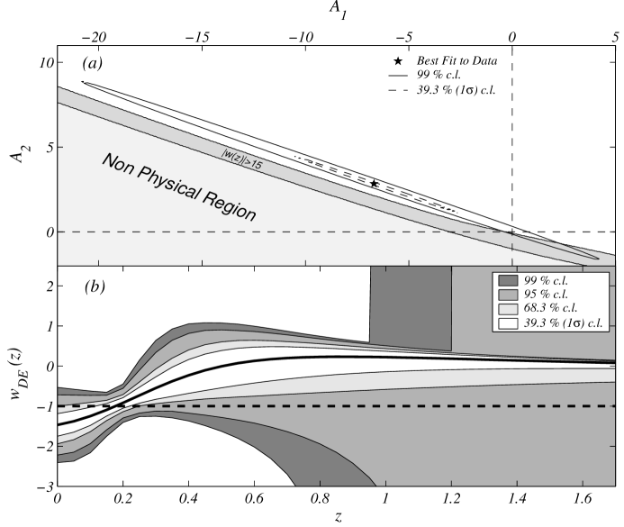
Figure 1: The results of the reconstruction of DE from the small data set, consisting of supernovae from Tonry et aland Barris et al. Panel (a) shows the $A_{1}-A_{2}$ parameter plane, where the best fit value to the data ($A_{1}=-6.68$ and $A_{2}=2.84$) is indicated by a star. The solid and dashed contours indicate the $99\%$ and 1$\sigma$ confidence levels (CL) respectively. In panel (b) the reconstructed equation of state parameter corresponding to the best fit (solid line) and various confidence regions are drawn. The obtained equation of state parameter is consistent with a cosmological constant at the $95\%$ CL, but not at the $68\%$ CL. Note that Alam et al report their confidence regions as 1$\sigma$ levels, i.e. as $\mathcal{L}_{max}-{1\over 2}$ in their maximum likelihood analysis. As two parameters are jointly fitted this corresponds only to a 39.3 % CL. The shown discontinuities in the $95\%$ and $99\%$ CL regions correspond to the contours crossing the dark shaded region in the $A_{1}-A_{2}$ plane in panel (a), where $w_{DE}(z)$ grows very rapidly.

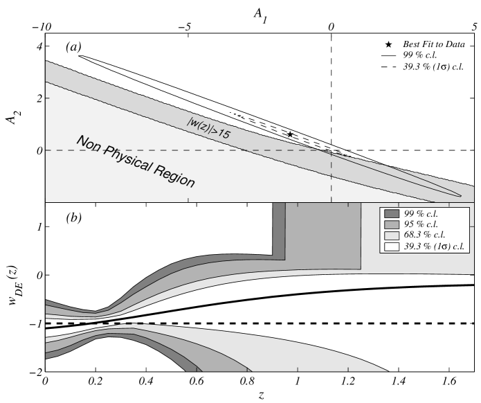
Figure 2: The results of the reconstruction of DE from the large data set, consisting of the small data set and $16$ additional high–z supernovae from Riess et al. In panel (a) the best fit values to this data set ($A_{1}=-1.44$ and $A_{2}=0.61$) is indicated by a star. The solid and dashed contours indicate the $99\%$ and 1$\sigma$ confidence levels (CL) contours respectively. Both CL contours cross the region in the parameter plane where $w_{DE}(z)$ blows up or diverges (dark gray). The equation of state obtained for this data set, shown in panel (b), is consistent with the cosmological constant not only at the $95\%$ CL, but also at the $68\%$ CL.

4 Analysis of the dark energy equation of state parameter

The unusual behaviour of the results in figure 1 and 2 appear since the dark energy equation of state parametrization (4) has a few peculiarities, which we discuss in this section.

4.1 Diverging equation of state parameter

The dark energy equation of state parameter will obviously diverge whenever the denominator in equation (4) vanishes. Regions in the parameter plane where $w_{DE}(z)$ blows up ($|w_{DE}|>15$) or diverges somewhere in the redshift interval $0\leq z\leq 1.8$ are shown in dark gray in e.g. panel (a) in figure 1. The point $A_{1}=A_{2}=0$, corresponding to the cosmological constant, lies very close to this region. If the best fit to data is near this point, the error in $w_{DE}(z)$ will blow up. Diverging equation of state parameter is the reason why the $95\%$ confidence region in e.g. figure 1(b) blows up.

4.2 High redshift limits and shrinking confidence regions

From equation (4) one can easily see that the parametrized equation of state depends on the order of the Taylor expansion at the high redshift limit. If, for instance, only the first order is considered, $w_{DE}\rightarrow-{\textstyle\frac{2}{3}}$ for high redshifts, while for the second order $w_{DE}\rightarrow-{\textstyle\frac{1}{3}}$. Since the proposed ansatz (1) is a truncated Taylor series we cannot expect equation (4) to be valid at very high redshifts. However, the effects of these high redshift limits are noticeable already at the moderate redshifts where we try to model DE. These limits are responsible for the shrinkage of the non–diverging confidence regions at high redshift (e.g., see the $68\%$ confidence region in figure 1(b)).

4.3 Stability of the dark energy equation of state parameter

The dark energy equation of state parameter described by equation (4) can be thought of as a family of curves, where each curve is parametrized by $\Omega_{M}$, $A_{1}$ and $A_{2}$. In this section we study the stability of these curves to perturbations in the parameters $A_{1}$ and $A_{2}$. Moreover, we will show that some curves in this family become more stable with redshift, with respect to these perturbations, while others become more unstable. The change $\delta w_{DE}$ in a curve, described by the parameters $A_{1}^{0}$ and $A_{2}^{0}$, due to small perturbations $\delta A_{1}$ and $\delta A_{2}$ is given by

$$\delta\!w_{DE}\approx\frac{\partial w_{DE}}{\partial A_{1}}(A_{1}^{0},A_{2}^{0})\delta\!A_{1}+\frac{\partial w_{DE}}{\partial A_{2}}(A_{1}^{0},A_{2}^{0})\delta\!A_{2}.$$ (8)

The curve that corresponds to the cosmological constant ($A_{1}=A_{2}=0$) becomes increasingly unstable due to perturbations as redshift increases,

$$\delta\!w_{\Lambda}\approx\frac{x}{3(1-\Omega_{M})}\delta\!A_{1}+\frac{2x^{2}}{3(1-\Omega_{M})}\delta\!A_{2}.$$ (9)

A curve that starts close to the line $w_{DE}(x)=-1$ will thus departure from this line with increasing redshift. Equation (4) can also make an exact reproduction of two types of topological defects. The equation of state of domain walls ($A_{0}=A_{2}=0$) grows stable to perturbations in $A_{1}$ with $z$, but not to perturbations in $A_{2}$

$$\delta\!w_{DE}\approx\frac{1}{3(1-\Omega_{M})x}\delta\!A_{1}+\frac{1}{3(1-\Omega_{M})}\left(x+\frac{1}{x}\right)\delta\!A_{2}.$$ (10)

The curve corresponding to cosmic strings ($A_{0}=A_{1}=0$) is stable to perturbations in both $A_{1}$ and $A_{2}$ at high redshifts

$$\delta\!w_{DE}\approx\frac{2}{3(1-\Omega_{M})}\left(\frac{1}{x^{2}}-\frac{1}{2x}\right)\delta\!A_{1}+\frac{2}{3(1-\Omega_{M})x^{2}}\delta\!A_{2}.$$ (11)

The curves corresponding to topological defects are thus very special. All other curves (except the one corresponding to the cosmological constant) approach one of these two curves as redshift increases. The effect of perturbations in $A_{1}$ and $A_{2}$ depends on the value of these parameters. This is in contrast to perturbations of linear parameterizations of $w_{DE}(z)$, e.g. $w_{DE}(z)=w_{0}+w_{1}z$, which are independent of parameter values. From the above discussion about the stability of $w_{DE}(x)$ with redshift, we see that the parameterization in equation (4) treats the cosmological constant unfairly in favour of other DE alternatives.

4.4 Forced evolution of the dark energy equation of state parameter

The parametrized equation of state parameter (4) will not only favour, but also “force” evolution. All curves, describing an evolving equation of state parameter, will cross at a certain redshift. At this redshift $z_{*}=x_{*}-1$, where $x_{*}=-A_{1}/2A_{2}$, the numerator and denominator are equal and the dark energy equation of state assumes the value $w_{DE}(z_{*})=-1$. The parameters $A_{1}$ and $A_{2}$, obtained by fitting supernova data to the ansatz (1), are highly correlated and the ratio $A_{1}/A_{2}$ is thus nearly constant. The value of this ratio depends on the slope of the CL contours in the $A_{1}-A_{2}$ plane which in turn is correlated with the assumed prior on the matter density $\Omega_{M}$. This implies that the location of the point $x_{*}=-A_{1}/2A_{2}$ is more or less independent of the parameters $A_{1}$ and $A_{2}$ for a given $\Omega_{M}$. The parametrization (4) of the equation of state parameter thus favours DE evolution. If the reconstructed equation of state at present is less (larger) than minus one it must have been larger (less) than minus one in the past. Any significant departure from the line $w_{DE}(x)=-1$ will hence force the reconstructed equation of state parameter to cross that line. Since most curves will pass through this point, the family of curves will have a waist centered at $x_{*}=-1/2k$, where $k$ denotes the slope of the CL contours in the $A_{1}-A_{2}$ plane. The transition redshift in e.g. figure 1 is $z_{*}\approx 0.2$ which corresponds to $k=-0.42$, in good agreement with the slopes of the ellipses in panel (a).

5 Simulations

To test the reliability of this way of reconstructing the dark energy we tried to recover a fiducial cosmology from simulated data sets generated using SNOC [13], a Monte–Carlo simulation package for high–z supernova observations . We generated $500$ data sets, each one consisting of $172$ supernovae with the same distribution of redshifts and magnitude errors as the small data set used in section 3. A flat universe with a cosmological constant $\Lambda$ and $\Omega_{M}=0.3$ was used as fiducial cosmology. The parameters $A_{1}$ and $A_{2}$ were fitted to each simulated data set with a fixed value of $\Omega_{M}$.

A scatter plot of best fit values to the simulated data sets is shown in figure 3. From this plot it is clear that the best fit values of the parameters $A_{1}$ and $A_{2}$ are highly correlated, as anticipated in section 4.4. Of the simulated data sets, $61.8\%$ were found to be consistent with the cosmological constant at the $68\%$ CL. These are indicated by full circles in the plot. Data sets not consistent with the cosmological constant at the $68\%$ CL, on the other hand, are indicated by open circles. The best fit to real data obtained in section 3 is indicated with a star in the expanded figure in figure 3. The expansion shows a region where simulated data sets have a reconstructed dark energy equation of state parameter similar to the one obtained from real data. The simulated data sets in this region are inconsistent with the fiducial cosmology at the $68\%$ CL. Figure 4 shows a few examples of $w_{DE}(z)$ reconstructed from simulated data sets. The reconstructed $w_{DE}(z)$ in panel (b) is almost indistinguishable from the one obtained from real data (see figure 1). Rapidly evolving equation of state parameters, resembling the behaviour of the result obtained from real data, can thus be obtained from simulated data sets in a $\Lambda$ cosmology ($w_{DE}=-1$) with the same distributions of redshifts and magnitude errors as the real set.

We also simulated $500$ data sets with the same distribution of redshifts and magnitude errors as the large data set used in section 3. Figure 5 shows a scatter plot of the best fit values to these simulations. In this case $64.9\%$ of the simulated data sets were consistent with the fiducial cosmology on the $68\%$ CL. As can be seen from figure 5, the $16$ additional high redshift supernovae decrease the spread of the best fit values.

To save computational time, a simplified fitting procedure was used in the reconstruction of $w_{DE}(z)$ from the simulated data sets, as $\Omega_{M}$ was kept fixed at the input value. The value of the matter density affects the slope of the confidence contour. By using a more realistic fitting procedure the spread of the best fit values would increase.

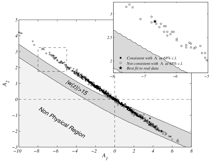
Figure 3: A scatter plot of the best fit central values of $A_{1}$ and $A_{2}$ to $500$ simulated data sets in a universe with a cosmological constant. The used cosmology corresponds to $A_{1}=A_{2}=0$. The best fit values $A_{1}$ and $A_{2}$ are evidently highly correlated. The plot in the upper right–hand corner is an enlargement of the part inside the dashed rectangle. The filled circles represent simulated data sets consistent at the $68\%$ confidence level with the fiducial cosmology. Data sets not consistent on this level are indicated by open circles. The star indicates the best fit value to real data. The dark energy equation of state reconstructed from data sets indicated by open circles in the neighborhood of the star, would thus look very similar to what we find from real data (see figure 1). Examples of $w_{DE}(z)$ reconstructed from a few of these data sets are shown in figure 4.

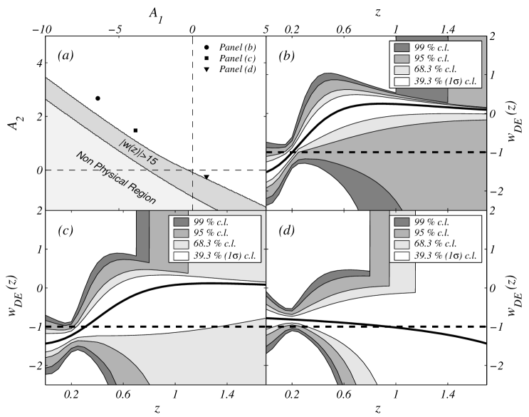
Figure 4: Examples of $w_{DE}(z)$ reconstructed from three different simulated data sets with a cosmological constant are depicted in panel (b), (c) and (d). The distributions of redshifts and magnitude errors for these data sets were the same as for the small data set used in section 3. Best fit values to the three data sets are indicated in panel (a). The reconstructed equation of state parameter evolves rapidly in all three cases, which indicates that metamorphosis is common also in a $\Lambda$–universe.

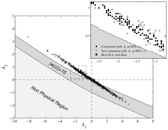
Figure 5: The same as in figure 3 but the simulated data sets contain $16$ additional supernovae at high redshifts. In this figure the star in the expanded figure indicates the best fit to the extended real data set. The additional supernovae have reduced the scatter of the best fit central values to the parameters $A_{1}$ and $A_{2}$.

6 Extended ansatz

As we have seen above, equation (4) involves some difficulties associated with the reconstruction of the dark energy equation of state parameter. Could an extension of the ansatz overcome these difficulties? Studies of an arbitrary power series describing the dark energy density might help us to answer this question

$$\rho_{DE}=\sum_{k}A_{k}x^{k},$$ (12)

where $k$ can be zero or any positive or negative integer. Perturbations in the parameters $A_{k}$ will cause a change in $\rho_{DE}$ that is independent of these parameters

$$\delta\!\rho_{DE}\approx\sum_{k}x^{k}\delta\!A_{k}.$$ (13)

A description of the density of dark energy in terms of a power series will thus not favour any particular model. The equation of state generated by a power series is given by (3)

$$w_{DE}(x)=-\frac{\sum_{k}\frac{3-k}{3}A_{k}x^{k}}{\sum_{k}A_{k}x^{k}}.$$ (14)

If only one coefficient in (14) is non–zero, $w_{DE}(x)$ assumes a constant value. The power series parametrization of the equation of state parameter is hence capable of reproducing a whole spectrum of constant $w_{DE}(x)$ separated by $\Delta w={\textstyle\frac{1}{3}}$

$$w_{DE}(x,A_{j}\neq 0,A_{k\neq j}=0)=-1+\frac{j}{3}.$$ (15)

The cosmological constant corresponds to $j=0$. The high redshift limit for a truncated power series with leading term $x^{n}$ resembles this spectrum

$$\lim_{x\rightarrow\infty}w_{DE}(x)=-1+\frac{n}{3}.$$ (16)

The change in $w_{DE}$ due to any perturbation of the parameters $A_{k}$ in the neighborhood of the cosmological constant ($A_{0}\neq 0$ and $A_{k\neq 0}=0$) is given by

$$\delta\!w_{DE}\approx\sum_{k}\frac{k}{3A_{0}}x^{k}\delta\!A_{k}.$$ (17)

The effect of perturbations in the parameters depends upon the leading term $A_{n}x^{n}$ in the power series. If $n$ is positive, the change in the equation of state parameter will increase with redshift. However, if $n$ is negative the change will decrease with redshift. In order to discriminate between the cosmological constant and evolving DE alternatives, we have to contrast this behaviour with the curves describing evolution. The perturbed equation of state parameter corresponding to non–zero $A_{k}$ at a high redshift ($x\gg 1$) with the leading term $A_{n}x^{n}$ is:

$$\delta\!w_{DE}\approx-\sum_{k}^{n-1}\frac{(n-k)}{3A_{n}}x^{-(n-k)}\delta\!A_{k}+\frac{A_{n-1}}{3A_{n}^{2}}x^{-1}\delta\!A_{n}.$$ (18)

The effects of perturbations decrease with redshift if $n$ is positive, or increase with redshift if $n$ is negative. This is the very opposite of the behaviour for the case of a cosmological constant. The instability problem discussed above can thus not be resolved by adding extra terms to the ansatz (1).

7 Discussion

The ansatz proposed by Alam et almay be useful for modelling the dark energy density, but its usefulness for revealing the nature of the DE seems limited. The parametrization of the dark energy equation of state parameter based on a truncated Taylor series involves a number of severe problems. Evolution is both favoured and forced by this parametrization. The cosmological constant is thus mistreated by the ansatz proposed in [1, 2]. Not even an extension of the ansatz seems to be able to overcome these difficulties.

The equation of state parameter expressed as in equation (4) also diverges in large regions of the parameter space. More data, which focus the solutions to the stable regions, may solve this problem. However, the region close to the point describing a universe with a cosmological constant will be in a disfavoured part of the parameter space.

The dark energy equation of state parameter reconstructed from the data sets presented in reference [3] and [4] is inconsistent with the cosmological constant at the $68\%$ confidence level. Simulations show that the rapidly changing behaviour of $w_{DE}(z)$ could also be expected with this ansatz for a $\Lambda$ universe. The scatter of the best fit parameters can be reduced if additional data points at high redshift are added to the simulated data sets. Our best fit to real data with $16$ additional high redshift supernovae was consistent with the cosmological constant at the $68\%$ confidence level.

We concluded that the suggested “model independent” method of reconstructing the dark energy equation of state parameter in [1], is in fact model dependent, and that the seemingly striking results are likely to be due to this deficiency.

References

- [1] Alam U, Sahni V, Saini T D and Starobinsky A A 2003 Preprint astro-ph/0311364
- [2] Alam U, Sahni V and Starobinsky A A 2004 JCAP 0406 008
- [3] Tonry J et al2003 Astrophys. J. 594 1
- [4] Barris B et al2004 Astrophys. J. 602 571
- [5] Riess A et al2004 Astrophys. J. 607 665
- [6] Knop R et al2003 Astrophys. J. 598 102
- [7] Wang Y and Mukherje P 2004 Astrophys. J. 606 654
- [8] Wang Y and Freese K 2004 preprint astro-ph/0402208
- [9] Wang Y and Tegmark M 2004 Phys. Rev. Lett. 92 241302
- [10] Huterer D and Cooray A 2004 preprint astro-ph/0404062
- [11] Daly R and Djorgovski S 2004 preprint astro-ph/0403664
- [12] Saini T D, Raychaudhury S, Sahni V and Starobinsky A A 2000 Phys. Rev. Lett. 85 1162
-
[13]
Goobar A, Mörtsell E, Amanullah R, Goliath
M, Bergström L and Dahlén T 2002
A & A 392 751 (
http://www.physto.se/~ariel/snoc)