A New calculation of the atmospheric neutrino flux in a 3-dimensional scheme.

Abstract

We have revised the calculation of the flux of atmospheric neutrinos based on a 3-dimensional scheme with the realistic IGRF geomagnetic model. The primary flux model has been revised, based on the AMS and BESS observations, and the interaction model updated to DPMJET-III. With a fast simulation code and computer system, the statistical errors in the Monte Carlo study are negligible. We estimate the total uncertainty of the atmospheric neutrino flux prediction is reduced to $\lesssim$ 10 % below 10 GeV. The ‘3-dimensional effects’ are found to be almost the same as the study with the dipole magnetic field, but the muon curvature effect remains up to a few tens of GeV for horizontal directions. The uncertainty of the absolute normalization of the atmospheric neutrino is still large above 10 GeV due to the uncertainty of the primary cosmic ray flux above 100 GeV. However, the zenith angle variation is not affected by these uncertainties.

I Introduction

The discovery of the neutrino oscillation from the study of atmospheric neutrinos is a one of the most important results in recent physical research sk (see also Refs. fukuda ; imb ; soudan2 ; macro , and Ref. KT for a review). The study is carried out by the comparison of theoretical calculation of the atmospheric neutrino flux and experimental data. Therefore, it is desirable that both theoretical and experimental studies are improved. The SuperKamiokande is improving the statistics and the accuracy steadily for experimental data. It is important to improve the theoretical prediction of the atmospheric neutrino flux also.

There have been some improvements in the theoretical prediction of the atmospheric neutrino fluxhkkm95 ; gaisser-new ; fluka-battis ; engel-hamburg ; hkkm-hamburg ; hkkm-tsukuba (see Ref. gaisser-honda for a review). These studies were useful to determine the flux ratios between different types of neutrinos and the variation over zenith angle with good accuracy, and establish neutrino oscillations and the existence of neutrino masses. We now wish to improve the accuracy of the absolute normalization as well as the ratio and directionality of the atmospheric neutrino fluxes for further studies.

In the time since our last comprehensive study of the atmospheric neutrino flux hkkm95 , knowledge of the primary cosmic ray has been improved by observations such as BESS bess and AMS ams below 100 GeV. There have also been theoretical developments in hadronic interaction models such as Fritiof 7.02 fritiof7.02 , FLUKA97 fluka and DPMJET-III dpmjet3 . Here, we adopt these revised primary flux and hadronic interaction models.

It has also been pointed out that the atmospheric neutrino flux calculated in a 3-dimensional scheme is significantly different from that calculated in a 1-dimensional scheme at low energies for near horizontal directions fluka-battis ; lipari-ge ; lipari-ew ; hkkm-dipole ; wentz ; liu ; bartol-3d . The 1-dimensional approximation has been widely used in the past, and was used in our previous calculation and others hkkm95 ; gaisser-new . This approximation is justified by the nature of hadronic interactions for calculations of high energy ($\gtrsim$ 10 GeV) atmospheric neutrino fluxes, but not at lower energies. With the computer resources then available, however, it was difficult to complete the calculation of atmospheric neutrino fluxes in a full 3-dimensional scheme within a tolerable length of the time. Some of 3-dimensional calculations employ approximations based on symmetry to circumvent the impact of limited computer resources. In Ref. fluka-battis , spherical symmetry is assumed, ignoring the magnetic field in the atmosphere, and in our previous 3-dimensional calculation hkkm-dipole we assumed an axial symmetry and used a dipole geomagnetic field model. Thus, a detailed calculation in a full 3-dimensional scheme without symmetry remains a challenging job.

We have developed a new and fast simulation code for the propagation of cosmic rays in the atmosphere to calculate the atmospheric neutrino flux in a full 3-dimensional scheme without having to assume symmetry. This fast simulation code and a fast computation system allow us to calculate the atmospheric neutrino flux with good accuracy over a wide energy region from 0.1 to a few tens of GeV, as is shown in this paper. The differences between 3-dimensional and 1-dimensional calculation schemes are similar to that we found in the study with a dipole geomagnetic field hkkm-dipole , and are small above a few GeV. The neutrino flux calculated in the 3-dimensional scheme is smoothly connected to the one calculated in the 1-dimensional scheme at a few tens of GeV. We are therefore able to discuss the atmospheric neutrino flux up to 10 TeV in this paper.

Although progress in our theoretical study of the atmospheric neutrinos flux has been reported partly elsewhere hkkm-hamburg ; hkkm-tsukuba , this is the first comprehensive report since 1995 hkkm95 .

II Primary cosmic ray flux model

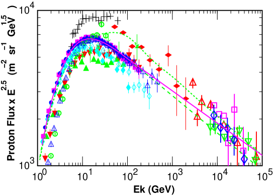
Figure 1: Primary cosmic ray observation and our model curves for protons at solar minimum. Crosses indicate data from Ref. webber , open circles indicate data from MASS mass , closed upward triangles LEAP leap , closed downward triangles IMAX imax , closed vertical diamonds CAPRICE-94 caprice94 , open vertical diamonds CAPRICE-98 caprice98 , closed circles BESS bess , closed horizontal diamonds AMS ams , open upward triangle BESS-TeV besstev , closed horizontal diamonds Ryan et al ryan , open downward large triangles JACEE jacee-p , open diamonds large RUNJOB runjob , open upward large triangles from Ivanenko et al. moscow , and open large squares from Kawamura et al. kawamura . The dashed line shows the spectrum calculated with Eq. 1 and Table 1, and the solid line shows that with the modification explained in the text. The dotted line is the proton flux model we used in Ref. hkkm95 .

The primary flux model we use is based on the one presented in Refs. gaisser-hamburg and gaisser-honda , in which the primary cosmic ray data below $\sim$ 100 GeV are compiled and parameterized with the fitting formula:

$$\phi(E_{k})\;=\;K\times\left(E_{k}\,+b\,\exp\left[-c\sqrt{E_{k}}\right]\right)^{-\alpha}\ .$$ (1)

where $\alpha,k,b,c$ are the fitting parameters. Although using the same fitting formula, the fitting parameters for nuclei heavier than helium are different in Refs. gaisser-hamburg and gaisser-honda . The parameters we used are taken from Ref. gaisser-honda and tabulated in table 1.

Table 1: Parameters for all five components in the fit of Eq. 1.

parameter/component	$\alpha$	$K$	$b$	$c$
Hydrogen (A=1)	2.74$\pm$0.01	14900$\pm$600	2.15	0.21
He (A=4)	2.64$\pm$0.01	600$\pm$30	1.25	0.14
CNO (A=14)	2.60$\pm$0.07	33.2$\pm$5	0.97	0.01
Mg–Si (A=25)	2.79$\pm$0.08	34.2$\pm$6	2.14	0.01
Iron (A=56)	2.68$\pm$0.01	4.45$\pm$0.50	3.07	0.41

However, the extension of this flux model for cosmic ray protons does not agree with emulsion chamber experiments above $\sim$ 10 TeV (the dashed line in Fig. 1). Therefore, we modified the power index above 100 GeV to $-$2.71, so that the fit passes through the center of the emulsion chamber experiments data (the solid line in Fig. 1). We also show the flux model for cosmic ray protons used in Ref. hkkm95 as the dotted line in Fig. 1. Other than the cosmic ray protons, we use the same flux model as Ref. gaisser-honda .

Note, we employ the superposition model for the cosmic ray nuclei, i.e., we consider a nucleus as the sum of individual nucleons, $Z$ protons and $A-Z$ neutrons. The validity of the superposition model was discussed in Ref. jengel based on the Glauber formalism of nucleus–nucleus collisions glauber . The authors showed the interaction mean-free-path of a nucleon in a nucleus is the same as a free nucleon, and concluded that the superposition model is valid for the calculation of time averaged quantities, such as the fluxes of atmospheric neutrinos and muons. A similar discussion was also presented in Ref. hkkm95 with the same conclusion.

III Hadronic interaction

For the hadronic interaction model, we are using theoretically constructed models which have been successfully applied to detector simulations in high energy accelerator experiments. In Ref. hkkm95 , we used NUCRIN nuc1 for 0.2 GeV $\leq E_{lab}\leq$ 5 GeV, FRITIOF version 1.6 fritiof1.6 for $5~{}{\rm GeV}\leq E_{lab}\leq 500~{}{\rm GeV}$, and an original code developed by one of us kasahara was used above 500 GeV. There were almost no improvements in the experimental study of the hadron interaction model of the multiple production, but there are noticeable improvements in the theoretical study, resulting in Fritiof 7.02 fritiof7.02 , FLUKA97 fluka , and DPMJET-III dpmjet3 .

To determine which is the better interaction model, we have used data on secondary cosmic ray muons mass-himu ; mass-himu2 ; caprice-himu ; caprice-himu2 ; bess-himu ; yamamoto ; abe1 and gamma-rays bets at balloon altitudes. The secondary cosmic rays at the balloon altitude are ideal for the study of the interaction model. They are approximately proportional to the air depth, and the ratio $[Flux/Depth]$ is determined almost only by the interaction and the flux of primary cosmic rays. On the other hand, the small statistics due to the small flux of secondary cosmic rays at balloon altitudes is the disadvantage for this study. The BESS 2001 flight is unique in this regard, as it measured the primary cosmic ray and muon fluxes simultaneously a little deeper in the atmosphere (4–30 g$/$cm²) than normal long duration flights, and collected a sufficient number of muons and primary protons. In Fig.2, we show the study made for muons observed by BESS 2001 abe1 . Although it is hard to discriminate between other interaction models, it is found the DPMJET-III gives the best agreement between calculation and observation (for details, see Ref. abe2 ). Note that the momentum range shown in Fig. 2 is from 0.4 to 10 GeV/c. and that primary cosmic rays with energies from 6 to 80 GeV are mainly responsible for the muons in this momentum range at the balloon altitude hkkm-hamburg ; gaisser-honda . Therefore, the study of the hadronic interaction model is for the primary cosmic rays in this energy region, corresponding to the neutrinos of 0.3–4 GeV.

For the wider energy region of primary cosmic rays, we may examine the hadronic interaction model using the observed muons at different altitudes and at sites with different cutoff rigidities. Note that at ground level the muon fluxes are available for a wider momentum range with good statistics. We are preparing a paper sanuki-mu for such a study with the muon fluxes observed by BESS motoki ; sanuki-mountain ; tanizaki , and so limit ourselves here to comment that the muon flux observed by BESS is reproduced with DPMJET-III with an accuracy of $\sim$ 5 % for the muons in the ‘important’ momentum range from 1 to a few tens of GeV/c for most cases. At ground level, the primary cosmic rays with energies from 20 to a few 100 GeV are responsible for the muons in this momentum range, corresponding to neutrinos of 1–10 GeV. This study was partly reported in Ref. hkkm-hamburg .

We do not use the original package of the hadronic interaction code in the calculation of atmospheric neutrino fluxes. We first carry out a computer experiment of the interaction of all kinds of primary or secondary cosmic rays with air-nuclei, using the original hadronic interaction code. Then, the ‘data’ are used to construct an inclusive interaction code, which reproduces the multiplicities and energy spectra of secondary particles of the original code. The inclusive interaction code violates the conservation laws for energy-momentum and other quantum numbers in a single interaction, but they are restored statistically. Note that for the secondary particles whose life time is shorter than $10^{-9}$ sec we record their decay products as the data. The experiment scans the energy region from 0.2 to $10^{6}$ GeV in kinetic energy, and is repeated typically 1,000,000 times for each kind of projectile and each injection energy.

For the energy distribution of secondary particles in the interaction, we fit the original distribution of $x$, defined as $x\equiv E_{k}^{sec}/E_{k}^{proj}$, with the combination of B-spline functions for each kind of projectile particle, each injection energy, and each kind of secondary. Then the inclusive code uses the B-spline-fit to reproduce the energy distribution of the secondary particle with a good accuracy. For the scattering angles, we calculate the average transverse momentum ($<p_{\perp}>$) for each kind of projectile, each injection energy, each kind of secondary, and each secondary energy. In the inclusive code, we sample the scattering angle ($\theta$) with the distribution function $\propto\exp(a\cdot\cos\theta)\cdot d\cos\theta$, where $a$ is determined so that $<p_{\perp}>$ is the same as the original interaction model. The $p_{\perp}$-distribution approaches $\propto\exp(-a^{\prime}\cdot p_{\perp}^{2})\cdot p_{\perp}dp_{\perp}$ and $a^{\prime}=\pi/(2<p_{|}>)^{2}$ for $p\gg$ 1 GeV/c. Note, the inclusive code constructed for DPMJET-III reproduces not only $<p_{\perp}>$ but also, approximately, the original $p_{\perp}$-distribution for $p_{\perp}<1$ GeV/c. There is a longer tail in the original $p_{\perp}$ distribution for larger $p_{\perp}$. However, since the number of secondary particles which have $p_{\perp}>1$ GeV/c is limited, they are not important in this study.

The constructed inclusive codes are typically $\sim$100 times faster than the original package. The fast computation is very important in the 3-dimensional calculation of the flux of atmospheric neutrinos, as well as the study of secondary cosmic rays. Note, however, the inclusive interaction code is only valid for the calculation of a time averaged quantity, such as the fluxes of atmospheric neutrinos and muons. The situation is similar to the superposition model for the nuclear cosmic rays.

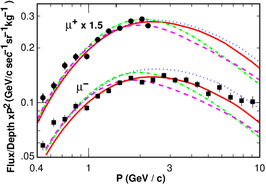
Figure 2: The quantity $[Flux/Depth]$ averaged over all the muon observation by BESS 2001 abe2 at balloon altitudes. The lines are the same quantities calculated by DPMJET-III (Solid line), Fritiof 1.6 (Dashed line), Fritiof 7.02 (dotted line), and FLUKA 97 (Dash dot),

IV Calculation Scheme

Except for the geomagnetic field model, the simulation scheme is similar to the previous 3-dimensional calculation hkkm-dipole in which we assumed a dipole geomagnetic field. In this calculation, we use the IGRF geomagnetic field model igrf with the 10th order expansion of spherical functions for the year 2000. As the geomagnetic field changes very slowly, the neutrino flux calculated for the year 2004 would not show a noticeable difference. We use the US-standard 1976 us_standard atmospheric model, as in the previous study. Note that for a study of the seasonal variations of atmospheric neutrino fluxes we need to use a more sophisticated and detailed atmospheric model nrlmsise00 .

We assume the surface of the Earth is a sphere with radius of $R_{e}=6378.180$ km. We also assume 3 more spheres; the injection, simulation, and escape spheres. The radius of the injection sphere is taken as $R_{inj}=R_{e}+100$ km, the simulation sphere as $R_{sim}=R_{e}+3000$ km, and the escape sphere as $R_{esc}=10\times$$R_{e}$. The sizes of the injection sphere ($R_{inj}$) and escape sphere ($R_{esc}$) are the same as in the previous study hkkm-dipole .

The cosmic rays are sampled on the injection sphere uniformly toward inward directions, following the given primary cosmic ray spectra. Before they are fed to the simulation code for propagation in air, they are tested to determine whether they can pass the rigidity cutoff, i.e., the geomagnetic barrier. For a sampled cosmic ray, the ‘history’ is examined by solving the equation of motion in the negative time direction. When the cosmic ray reaches the escape sphere without touching the injection sphere again in the inverse direction of time, the cosmic ray can pass through the magnetic barrier following the trajectory in the normal direction of time. In the 1-dimensional calculation we normally prepare a cutoff table for each neutrino detector site beforehand, but it is practically impossible to construct such a table for the 3-dimensional calculation. Note, all the nucleons carried by the cosmic ray nuclei are treated as protons with double rigidity ($=$ momentum for protons), before the first interaction with an air-nucleus and in the rigidity cutoff test.

The propagation of cosmic rays is simulated in the space between the surface of Earth and the simulation sphere. When a particle enters the Earth, it loses its energy very quickly, and generates neutrinos with energy less than 100 MeV only. Therefore, we discard such particles as soon as they enter the Earth, as most neutrino detectors which observe atmospheric neutrinos do not have sensitivity below 100 MeV.

For secondary particles produced in the interaction of a cosmic ray and air-nucleus, there is the possibility that they go out and re-enter the atmosphere and create neutrinos with energy $\sim$1 GeV. Therefore, too small a simulation sphere may miss such secondary particles. On the other hand, it is very time consuming to follow all the particles out to distances far from the Earth. In the previous study, we took the radius of simulation sphere to be $R_{sim}=$$R_{e}+300$ km, and showed that this is sufficient to calculate the neutrino flux to within a accuracy of $\sim$1 % from an analysis of the neutrino production time after the first interaction nu2002 . In this paper, however, we adopt a radius for the simulation sphere of $R_{sim}=$$R_{e}+3000$ km for greater accuracy, since we found the average computation time for a primary cosmic ray does not increase that rapidly up to a simulation sphere of this size. Regarding the size of simulation sphere, we study the neutrino production time after the injection of the primary cosmic ray in Sec. IV.1.

We ‘observe’ the neutrino at the surface of the Earth, and the size of the ‘virtual detector’ is closely related to the accuracy of the calculated flux and computation time. With too large a virtual detector, the average observation conditions, such as the dependence on the geomagnetic field, may differ from the real site. However, with too small a virtual detector, it is difficult to collect a sufficient number of neutrinos within a reasonable computation time. In the previous study, we assumed an axial symmetry with dipole geomagnetic field, and considered a belt around the Earth as the virtual detector. For the more realistic geomagnetic filed model IGRF, we consider a localized virtual detector, the surface of the Earth inside a circle with the radius of $\sim$ 1117 km (center angle of $10^{\circ}$) around the target detector. The virtual detector is $\sim 1/6$ the size of the previous one.

Note, we placed many virtual detectors on the Earth corresponding to the existing neutrino detectors, and recorded neutrinos for each detector at the same time. However, we only show the results for the virtual detectors placed at Kamioka and North America in this paper, as they are good examples of a low magnetic latitude and a high magnetic latitude, respectively. The fluxes for Soudan and Sudbury are almost identical, and we refer to them here as North America.

IV.1 Neutrino production time.

Before showing the resulting atmospheric neutrino flux, we would like to introduce some interesting quantities; the neutrino production time and the impact parameter of primary cosmic rays. These quantities provide important hints for the efficient calculation of atmospheric neutrino fluxes in the 3-dimensional scheme.

First, we show the study of neutrino production time. Before the calculation of atmospheric neutrino fluxes, we studied the neutrino production time to optimize the size of simulation sphere. Note, the radius of the simulation sphere used in this study is $R_{sim}$ = 10 $\times$ Re = 63,781.80 km, and so neutrinos produced within $t_{free}=2\times(R_{sim}-R_{inj})/c\sim 0.4$ sec after the injection of cosmic ray at the injection sphere are absolutely free from the boundary, by the naive discussion of the causality.

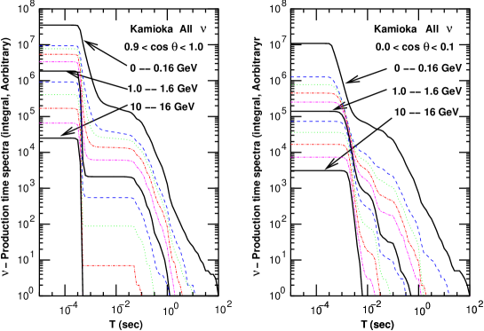
Figure 3: Integral production time distribution for the atmospheric neutrinos observed at Kamioka. For the neutrino energies, we divide each decade into 5 bins, and show the production time spectra in solid, dashed, dash-dot, dash-dot-dot, and dash–3-dot lines.

We show the integral distribution of the neutrino production time for neutrinos observed in Kamioka in Fig. 3. The production time is measured after the injection of the cosmic ray at the injection sphere. We find that $t_{free}$ for $R_{sim}=$$R_{e}+3000$ km ($\sim$ 20 msec) is large enough to calculate the flux of atmospheric neutrinos with an accuracy much better than 1%. It is interesting that there is a second peak at $\sim$0.1 sec due to the albedo particle reported by AMS.

We used $R_{sim}=$$R_{e}+300$ km in the previous study hkkm-dipole , and reported that this $R_{sim}$ is sufficient for calculation of atmospheric neutrino fluxes with an accuracy of $\sim$1% nu2002 . Note there is a $\sim$0.3 msec time offset in the production time after the injection for vertical directions, and $\sim$3 msec time offset for horizontal directions. Considering that the offset time is different for each injected cosmic ray, the study of the production time after the first interactions of cosmic rays requires a more sophisticated study than the present one. We can expect much better accuracy with $R_{sim}=$$R_{e}+3000$ km.

The same study has been carried out for other neutrino detector sites. However, the distributions are similar to that of Kamioka except for the height and position of the second peak. The second peak is lower and at larger production time for the higher latitude site.

IV.2 Impact parameter of the primary cosmic rays.

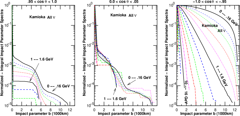
Figure 4: Normalized integral impact parameter distribution of the primary cosmic rays which produce neutrinos observed at Kamioka. Each decade of neutrino energy is divided into 5 bins, and the impact parameter spectra are shown by solid, dashed, dash-dot, dash-dot-dot, and dash–3-dot lines.

Here, we study the impact parameter of cosmic rays which produce a neutrino passing through the detector. When the cosmic ray produces a neutrino going through a virtual detector, the impact parameter ($b$) is calculated against the contact point of the neutrino and the surface of Earth for the input primary cosmic ray at the injection sphere.

The impact parameter distributions are normalized and integral form are shown for Kamioka in Fig. 4. As expected, the impact parameters of downward going neutrinos are distributed in a narrow region near $b=0$, while those of upward going neutrinos are widely distributed. However, we find the distribution shrinks to $b=0$ as the neutrino energy increases, and for neutrinos with energy $>$ 10 GeV, most neutrinos ($>$ 99%) are produced by primary cosmic rays with $b<$ 1000 km.

The study of impact parameters can be used to accelerate the calculation of the atmospheric neutrino flux above $\gtrsim$ 10 GeV. Selecting an impact parameter for primary cosmic rays of $<$ 2000km at the injection results in atmospheric neutrino flux calculations $\sim$30 times faster than the original calculation scheme explained above. We use this acceleration technique for the neutrino flux above 10 GeV.

In Kamioka, it is found that the impact parameter distribution has a structure at 5–6000 km for the vertical directions, and 3–5000 km for horizontal directions. This is considered again to be the effect of the albedo particles observed by AMS. However, the contribution is small ($\ll$ 1%). The same study has been done for other neutrino detector sites. However, the concentration of the impact parameter distribution to $b=0$ is quicker than Kamioka for downward going neutrinos, as they site at higher geomagnetic latitudes than Kamioka. For upward going neutrinos, the impact parameter distribution is almost the same for all the sites.

V The flux of atmospheric neutrinos

Without limiting the impact parameter, we sampled 307,618,204,971 cosmic ray nucleons before the rigidity cutoff test, and simulated the propagation in air for 116,086,900,000 nucleons with kinetic energy $>$ 1 GeV, or equivalently all the cosmic rays with $E_{k}/A>1$ GeV arrive on the injection sphere in $8.07\times 10^{-8}$ second. Limiting the impact parameter, we sampled 415,711,823,606 cosmic ray nucleons before the rigidity cutoff and impact parameter test, and simulated the propagation in air for 25,413,045,195 nucleons with kinetic energy $>$ 10 GeV or equivalently all the cosmic rays with $E_{k}/A>10$ GeV arrive on the injection sphere in 1.4 micro second. Note the flux tables for Kamioka, Gran Sasso, and North America calculated in this study are available at http://www.icrr.u-tokyo.ac.jp/~mhonda.

In this section we present the characteristic features of the atmospheric neutrino flux calculated in the 3-dimensional scheme (3D) and compare them with those calculated in the 1-dimensional scheme with the same primary cosmic ray flux and interaction model. To study the differences due to the interaction model and the calculation scheme in 3-dimensional calculation, we also compare the atmospheric neutrino flux calculated in Ref. fluka-battis (FLUKA), and the one calculated in our previous 3-dimensional study with the dipole magnetic field hkkm-dipole (DIPOLE). Note, the interaction model used in DIPOLE is the same as Ref. hkkm95 . Interaction models and the geomagnetic field models used in the calculations are summarized in Table 2.

For Kamioka and Gran Sasso, we calculated the atmospheric neutrino fluxes considering the effect of the surface structure (mountains) above the neutrino detectors. However, in the following studies, we use the neutrino flux calculated for a flat detector at sea level, i.e., ignoring surface structure, to see the differences due to the calculation schemes.

Table 2: Interaction and geomagnetic field models in the calculations.

Calculation	Int. Model	Geomagnetic Field	Geomagnetic field
		(Rigidity cutoff)	(In air)
3D	DPMJET-III	IGRF	IGRF
FLUKAfluka-battis	FLUKA	IGRF	None
DIPOLEhkkm-dipole	Fritiof 1.6 base	Dipole	Dipole
1D	DPMJET-III	IGRF	none

V.1 Zenith angle dependence of the neutrino flux

The most prominent difference between 3-dimensional and 1-dimensional atmospheric neutrino flux calculations is the horizontal enhancement at low energies. (For the origin of the horizontal enhancement, see Refs.gaisser-honda ; lipari-ge ; hkkm-dipole ) We compare the zenith angle dependences of atmospheric neutrino fluxes calculated in the 3D, 1D, FLUKA, and DIPOLE cases for Kamioka (Fig. 5) and North America (Fig. 6), integrating over several energy bins and averaging over azimuth angles.

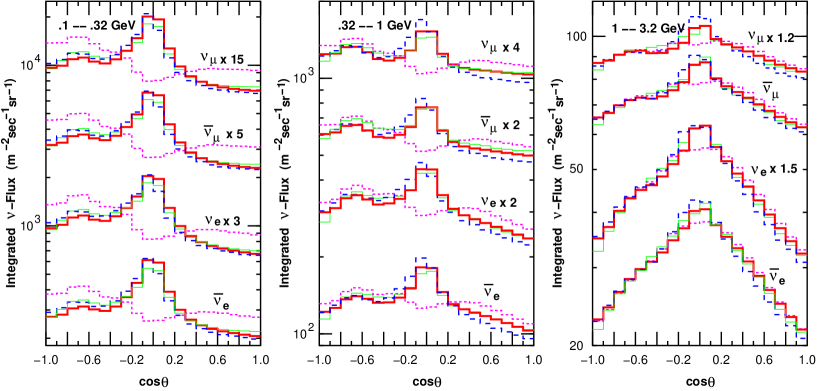
Figure 5: Zenith angle dependence of the atmospheric neutrino flux at Kamioka in 3 energy bins. For the azimuthal directions, averages are taken. The thick solid lines are for 3D, dotted lines for 1D, dashed lines for FLUKA, and thin solid lines for DIPOLE.

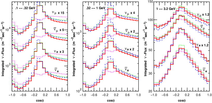
Figure 6: Zenith angle dependence of the atmospheric neutrino flux at North America in 3 energy bins. For the azimuthal directions, averages are taken. The notation for lines is the same as Fig. 5.

In these figures, we see the horizontal enhancements in 0.1–0.32 GeV and 0.32–1 GeV energy bins for all the 3-dimensional calculations. On the other hand, the flux near horizontal directions is rather smaller than neighboring directions in the 1D case due to the high cutoff rigidities. In the 1–3.2 GeV energy bin, the differences between the calculations are small. To study the difference of zenith angle dependences of neutrino fluxes due to the calculation scheme, we normalize each flux by the omni-directional flux average and depict the ratio to the 3D case in Figs 7 and 8 as a function of zenith angle.

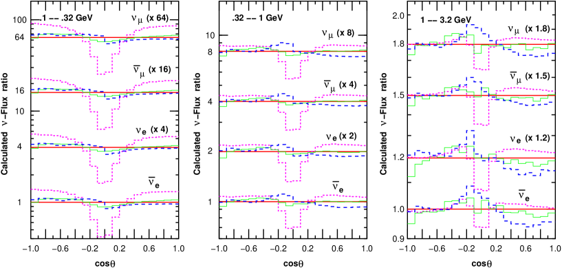
Figure 7: The normalized ratio of each flux to the 3D case as a function of zenith angle, for Kamioka. Dotted lines are for 1D, dashed lines for FLUKA, and thin solid lines for DIPOLE.

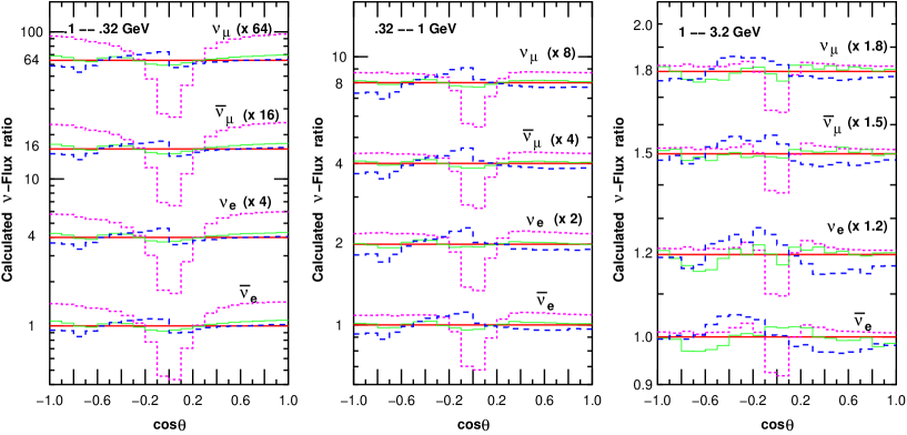
Figure 8: The ratio of atmospheric neutrino fluxes calculated by 1D, FLUKA, and DIPOLE for North America to that from the 3D case. The notations are the same as for Fig. 7.

In these figures, we find that the horizontal enhancement still exists in the 1–3.2 GeV energy bin, but that it decreases rapidly with neutrino energy. The difference at near horizontal directions is more than 50 % in 0.1–0.32 GeV bin, but it reduces to $\lesssim$ 10% in 1–3.2 GeV bin, for all kinds of neutrino.

The differences among the 3-dimensional calculations (3D, FLUKA, DIPOLE) are small, especially that between 3D and DIPOLE. However, the amplitude of the horizontal enhancement in DIPOLE is clearly slightly smaller than that in the 3D calculation. This is thought to be due to the difference of interaction model, especially to the average transverse momentum of secondary mesons. Note, the $<P_{t}>$ of pions is 0.289 GeV$/$c in DPMJET-III, while it is 0.256 GeV$/$c in Fritiof 1.6 for P + Air interactions at $E_{lab}=$10 GeV. The difference between 3D and FLUKA is asymmetric below and above the horizontal direction ($\cos\theta=0$). It is difficult to deduce differences in the interaction model in this comparison.

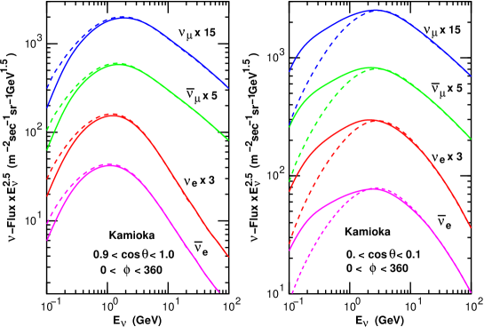
Figure 9: Atmospheric neutrino fluxes at Kamioka for 3D and 1D, averaged over azimuth angles. The left panel shows the comparison for vertical directions, and the right panel for horizontal directions. The solid lines show the 3D results and the dashed lines the 1D results.

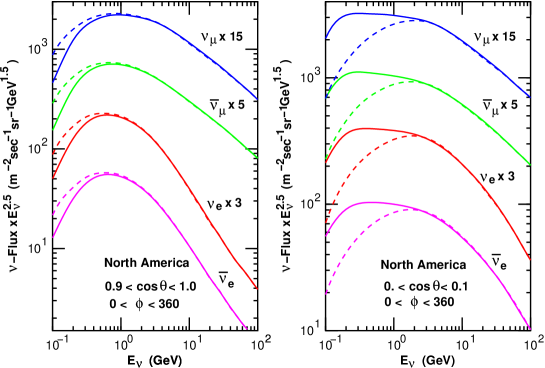
Figure 10: Atmospheric neutrino fluxes at North America for 3D and 1D, averaged over azimuth angles. The left panel shows the comparison for vertical directions, and the right panel for horizontal directions. The solid lines show the 3D results and the dashed lines the 1D results.

To see the energy dependence of the horizontal enhancement more clearly, we compared the 3D and 1D energy spectra for vertical and horizontal directions averaging over azimuth angles in Figs. 9 (Kamioka) and 10 (North America). We find the differences disappear at $\sim$1 GeV for vertical directions, and $\sim$3 GeV for horizontal directions, for all neutrinos.

Moreover, we find the fluxes averaged over all directions for 3D and 1D cases are very close to each other, even at low energies. Averaging the neutrino fluxes in Figs  5 and 6 over zenith angles, the 3D/1D ratios are tabulated in table 3. They agree with each other to within a few % in all cases.

Table 3: 3D/1D ratio for the all-direction average of atmospheric neutrino flux.

Eν(GeV)	$\nu_{\mu}$	$\bar{\nu}_{\mu}$	$\nu_{e}$	$\bar{\nu}_{e}$
Kamioka
0.1 – .32	0.979	0.980	0.970	0.978
.32 – 1.0	0.997	1.000	0.999	0.992
1.0 – 3.2	0.983	0.984	0.982	0.975
North America
0.1 – .32	1.036	1.035	1.028	1.025
.32 – 1.0	1.019	1.020	1.021	1.014
1.0 – 3.2	0.992	0.990	0.989	0.985

V.2 East–West effect

Here, we use the 3D and 1D fluxes only, since they are calculated under the same conditions (except for the 1- or 3-dimensional calculation scheme). Contrary to the quantitative agreements between 3D and 1D above a few GeV in the azimuthally averaged fluxes, they are quite different when the azimuth angles are limited to East or West directions, even at higher energies ($\sim$ 10 GeV).

We depict the 3D and 1D atmospheric neutrino fluxes arriving horizontally ($0.<\cos\theta<0.1$) from the East ($60^{\circ}<\phi<120^{\circ}$), and West ($240^{\circ}<\phi<300^{\circ}$) for Kamioka (Fig. 11) and North America (Fig. 12), where we measure the azimuth angle from South ($\phi=0$), and $\phi=90^{\circ},180^{\circ},270^{\circ}$ are East, North, and West directions respectively.

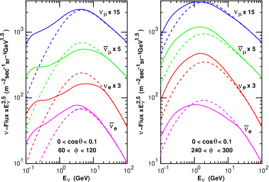
Figure 11: The flux of horizontal ($0.<\cos\theta<0.1$) atmospheric neutrinos arriving from the East ($60^{\circ}<\phi<120^{\circ}$, Left), and West ($240^{\circ}<\phi<300^{\circ}$, Right) directions at Kamioka. The solid lines show the result of the 3D calculation and the dashed line the 1D case.

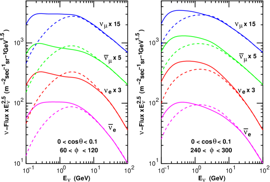
Figure 12: The flux of horizontal ($0.<\cos\theta<0.1$) atmospheric neutrinos arriving from the East ($60^{\circ}<\phi<120^{\circ}$, Left), and West ($240^{\circ}<\phi<300^{\circ}$, Right) directions at North America. The solid lines show the result of the 3D calculation and the dashed line the 1D case.

The differences in the fluxes from the 3D and 1D calculations for different kinds of neutrinos may be classified into two groups, $\nu_{\mu}$ and $\bar{\nu}_{e}$, and $\bar{\nu}_{\mu}$ and $\nu_{e}$. The former group are the decay products of $\mu^{-}$, and the latter are the decay products of $\mu^{+}$. The geomagnetic field deflects $\mu^{+}$’s toward the same direction as for primary cosmic rays. Therefore, it enhances the East and West differences of the $\bar{\nu}_{\mu}$ and $\nu_{e}$ fluxes caused by the rigidity cutoff. On the other hand, the geomagnetic field works on the $\mu^{-}$’s in the opposite direction to that for primary cosmic rays. Therefore, it reduces the East and West differences for the $\nu_{\mu}$ and $\bar{\nu}_{e}$ fluxes caused by the rigidity cutoff lipari-ew . In the Figs. 11 and 12, we mainly see the horizontal enhancement in the neutrino energies $\lesssim$ 1 GeV in the difference of 3D and 1D. For $\gtrsim$ 1 GeV, however, the muon curvature in the geomagnetic field is a larger effect than the horizontal enhancement, and this extends to several tens of GeV for near horizontal directions.

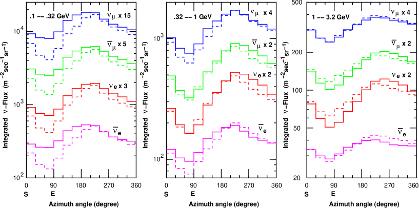
Figure 13: Azimuth angle dependence of the atmospheric neutrino flux at Kamioka, averaged over the zenith angle range $-0.5<\cos\theta<0.5$. The solid lines show the 3D result and the dashed lines the 1D result.

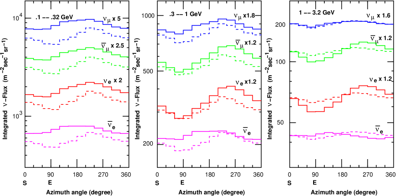
Figure 14: Azimuth angle dependence of the atmospheric neutrino flux at North America, averaged over the zenith angle range $-0.5<\cos\theta<0.5$. The solid lines show the 3D result and the dashed lines the 1D result.

Table 4: Max/Min ratio in Figs. 13 and  14 as the amplitude of the azimuthal angle variation.

Eν(GeV)	$\nu_{\mu}$	$\bar{\nu}_{\mu}$	$\nu_{e}$	$\bar{\nu}_{e}$	$\nu_{\mu}$	$\bar{\nu}_{\mu}$	$\nu_{e}$	$\bar{\nu}_{e}$
	Kamioka, 3D				Kamioka, 1D
0.1 – .32	2.27	2.51	2.75	2.03	4.13	4.13	4.36	3.85
.32 – 1.0	2.27	2.82	3.22	1.98	2.73	2.76	2.98	2.65
1.0 – 3.2	1.58	2.00	2.42	1.42	1.61	1.63	1.80	1.61
	North America, 3D				North America, 1D
0.1 – .32	1.26	1.33	1.40	1.19	1.47	1.48	1.54	1.41
.32 – 1.0	1.20	1.39	1.49	1.11	1.27	1.28	1.31	1.26
1.0 – 3.2	1.07	1.25	1.35	1.07	1.08	1.09	1.12	1.09

The muon curvature effect should be seen in the azimuthal variation of the atmospheric neutrino fluxes. We show the integrated azimuthal angle dependence in the same energy bins as in Sec. V.1 for Kamioka (Fig. 13) and North America (Fig. 14). Also we tabulated the ratio of maximum to minimum fluxes in the figures in Table 4, to see the variation amplitude. In the 1D case, the amplitudes are similar to each other for all kinds of neutrinos in each energy bin. This is because the 1D azimuthal variation is caused by the rigidity cutoff of the primary cosmic rays. In the 3D case, the amplitudes are different among the different kinds of neutrino even in the same energy bin. The amplitudes of $\nu_{\mu}$ and $\bar{\nu}_{e}$ are suppressed, while those of $\bar{\nu}_{\mu}$ and $\nu_{e}$ are enhanced, except for the lowest energy bin of 0.1–0.32 GeV. In the lowest energy bins, smearing suppresses the 3D azimuth angle dependence.

Note that $\nu_{e}$ has the largest amplitude among all $\nu$’s in 3D. This is because about $1/2$ of the $\bar{\nu}_{\mu}$’s are created by pion decay directly, while all the $\nu_{e}$’s are created by $\mu$-decay at these energies. It is noteworthy that the amplitude of $\nu_{e}$ in the 1–3.2 GeV energy bin is still large. This is important for the experimental confirmation of the effect of muon curvature, because the determination of the arrival direction is better for higher energy neutrinos.

Generally speaking, the azimuthal angle dependence of atmospheric neutrinos at high magnetic latitude sites such as North America is smaller than that at low magnetic latitude sites such as Kamioka because the rigidity cutoff is too low. However, we find in Fig. 14 and Table 4 that the difference in the azimuthal angle dependence of atmospheric neutrinos between 3D and 1D due to the muon curvature is similar to that for the low magnetic latitude site.

VI Neutrino fluxes at higher energies

In this section, we study the atmospheric neutrino flux at higher energies than in Sec. V. First, we note that the atmospheric neutrino fluxes above 10 GeV have a much larger uncertainty than those below 10 GeV. The main reasons are the uncertainties in the primary cosmic rays and the hadronic interaction model at energies above 100 GeV. As the difference between the neutrino fluxes calculated by 3-dimensional and 1-dimensional schemes are very small at the target energies here, we include the 1-dimensional calculations from Refs. hkkm95 (HKKM95) and gaisser-new (BARTOL) in this comparison, and plot them in Fig. 15. Note that, as the 1D results are almost the same as the 3D case in this energy region, and are identical above 100 GeV, they are referred just as this work in this section. Since the energy region available in the DIPOLE case is limited to below 10 GeV, it is omitted from the comparisons.

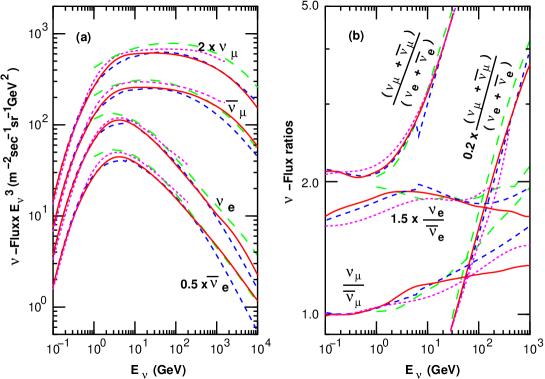
Figure 15: (a) Atmospheric neutrino fluxes averaged over all directions. (b) Flux ratios $(\nu_{\mu}+\bar{\nu}_{\mu})/(\nu_{e}+\bar{\nu}_{e})$, $\nu_{\mu}/\bar{\nu}_{\mu}$ and $\nu_{e}/\bar{\nu}_{e}$. Solid lines are for this work, dotted lines for HKKM95, dashed lines for FLUKA, and long dashed lines for BARTOL.

The larger fluxes in HKKM95 and BARTOL are due to the larger primary flux model used in HKKM95 (Fig. 1) and by the harder secondary spectrum in the hadronic interaction model (TARGET-I) used in BARTOL. We note that the ratios $(\nu_{\mu}+\bar{\nu}_{\mu})/(\nu_{e}+\bar{\nu}_{e})$ obtained for different calculations are very close. The agreement among the different calculations is well within 5 % at most energies. However, the ratios $\nu_{\mu}/\bar{\nu}_{\mu}$ and $\nu_{e}/\bar{\nu}_{e}$ show larger differences. The differences of $\nu_{e}/\bar{\nu}_{e}$ and $\nu_{\mu}/\bar{\nu}_{\mu}$ above a few GeV are caused by differences in the pion and kaon productions and their charge ratios in interactions above a few tens of GeV. In particular, $\nu_{e}/\bar{\nu}_{e}$ and $\nu_{\mu}/\bar{\nu}_{\mu}$ above 100 GeV are related to the kaon production in the hadronic interaction at energies above 1 TeV. Note it is still difficult to examine the hadronic interaction model at these energies.

Next, we study the zenith angle variation of the atmospheric neutrino flux at energies $\gtrsim$ 10 GeV with the quantity defined by

$$I_{n}(\cos\theta)=\int_{E1}^{E2}E_{\nu}^{n}{dN_{\nu}\over dE_{\nu}}(\cos\theta)dE_{\nu}\ .$$ (2)

The neutrino interaction cross section increases approximately in proportion to the neutrino energy. Therefore, $I_{1}(\cos\theta)$ is approximately proportional to the rate of neutrino events categorized as vertex contained and stop-muon events. High energy muon neutrinos are also observed, arising from muons produced in the rock. In this case, the neutrino observation probability is proportional to the multiple of $[muon\ range]\times[neutrino\ cross\ section]$. The muon range is approximately proportional to the muon energy below several 100 GeV, where the energy loss is dominated by ionization. The event rate is approximately proportional to $I_{2}(\cos\theta)$. Above $\sim$ 500 GeV, the muon energy loss is dominated by radiative processes paircreation , and the relation fails.

$I_{1}(\cos\theta)$ is calculated with $E_{1}=3.2$ GeV and $E_{2}=1000$ GeV, and is shown in the left panel of Fig. 16 for this work, HKKM95, BARTOL and FLUKA. Note, the median energy is $\sim$ 6 GeV in this integration over all the fluxes. We also depicted the normalized ratio of each flux to this work in the right panel of Fig. 16. As the atmospheric neutrino flux is expected to be symmetric above and below $\cos\theta=0$, we depicted the lower half ($\cos\theta<0$) only. Although there are large differences among theses calculations in the absolute values, the differences of normalized fluxes are small, particularly for $\nu_{\mu}$ and $\bar{\nu}_{\mu}$ ($\lesssim$ 3 %).

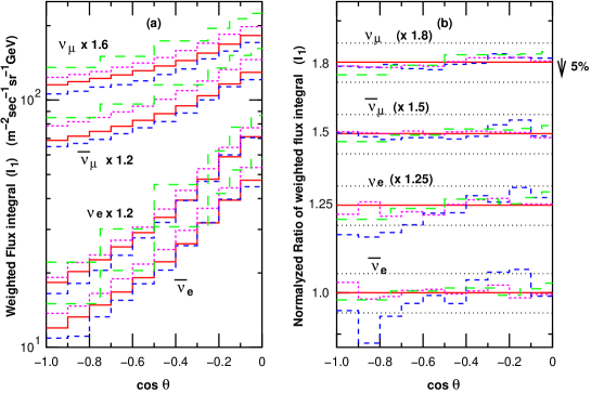
Figure 16: (a) Zenith angle variation of $I_{1}$ defined by Eq.2. (b) The normalized ratio of $I_{1}$ of each flux to this work as a function of zenith angle. The solid lines are for this work, dotted lines for HKKM95, dashed lines for FLUKA, and long dashed lines for BARTOL in both panels.

In Fig. 17, we show the zenith angle variation of $I_{2}$ with $E_{1}=10$ GeV and $E_{2}=1000$ GeV for this work, HKKM95, BARTOL, and FLUKA for $\nu_{\mu}$ and $\bar{\nu}_{\mu}$ fluxes. The median energy is $\sim$ 100 GeV. We find a large difference in absolute values as is expected from the left panel of Fig. 15. However, the differences are small when they are normalized. The ratio of the normalized weighted integral $I_{2}$ is shown as a function of zenith angle in the right panel of Fig. 15. The differences in normalized fluxes are $\lesssim$ 3 %.

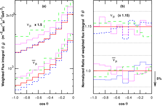
Figure 17: (a) Zenith angle variation of $I_{2}$ defined by Eq.16. (b) Normalized ratio of $I_{2}$ of each flux to this work as a function of zenith angle. The solid line is for this work, dotted line for HKKM95, dashed line for FLUKA, and long dashed line for BARTOL in both panels.

As is seen in the left panel of Fig. 15, the ratios $\nu_{\mu}/\bar{\nu}_{\mu}$ and $\nu_{e}/\bar{\nu}_{e}$ differ significantly between the calculations above 10 GeV. This is due to differences in the pion and kaon productions in the interaction model used by the different calculations. For example the multiplicity for kaons in DPMJET-III is almost 20% larger than that of FLUKA 97 at 1 TeV. Note, the interaction model used in FLUKA is developed by the authors of FLUKA 97. Despite these differences in the interaction models, the zenith angle dependences of atmospheric neutrinos show good agreement between the different calculations.

VII Production height of atmospheric neutrinos.

In the analysis of neutrino oscillations, the distance from the point at which the neutrino originates to the detector plays an essential role in determining $\Delta m^{2}_{23}$. To estimate the distance, the arrival zenith angle is used. However, the arrival zenith angle does not determine the distance uniquely, but gives a probability distribution for the distance. In this section, we study the neutrino production height distribution for a given zenith angle. As we assumed the surface of the Earth is a sphere, the distance and production height are related by the formula:

$$d=\sqrt{(h^{2}+2R_{e}h)+(R_{e}\cos\theta)^{2}}-R_{e}\cos\theta~{}~{},$$ (3)

where $h$ is the height, $R_{e}$ is the radius of the Earth, and $d$ is the distance. Note, the production height distribution changes its shape slowly as the zenith angle varies, while the distance distribution changes its shape very quickly near horizontal directions. Therefore, the study of production height distribution is more robust than the direct study of the distance distribution.

In the experimental analysis, the neutrino events are generally grouped in zenith angle bins irrespective of their azimuthal directions. Also, it is difficult to distinguish $\nu$ from $\bar{\nu}$ in current experiments. Therefore, we study the production height averaged over the azimuthal angles and for the sum of $\nu_{\mu}$ and $\bar{\nu}_{\mu}$, and $\nu_{e}$ and $\bar{\nu}_{e}$.

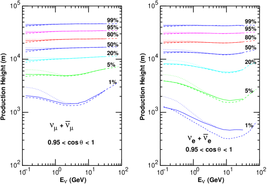
Figure 18: The neutrino production height at near-vertical directions for $\nu_{\mu}$ and $\bar{\nu}_{\mu}$ (left) and $\nu_{e}$ and $\bar{\nu}_{e}$ (right). The fixed accumulated probabilities of 1 % 5 %, 20 %,50 %,80 %, 95 %, and 99 % for the production height are shown as a function of the neutrino energy. The solid lines are for 3D at Kamioka, dashed lines for 1D at Kamioka, and dotted lines for 3D at North America.

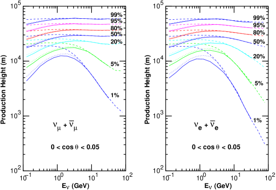
Figure 19: The neutrino production height at near-horizontal directions for $\nu_{\mu}+\bar{\nu}_{\mu}$ (left) and $\nu_{e}+\bar{\nu}_{e}$ (right). The fixed accumulated probabilities of 1 % 5 %, 20 %,50 %,80 %, 95 %, and 99 % for the production height are shown as a function of the neutrino energy. The solid lines are for 3D at Kamioka, dashed lines for 1D at Kamioka, and dotted lines for 3D at North America.

We show the neutrino production height distribution for vertical directions (Fig. 18) and for horizontal directions (Fig. 19). In the figures, we depict the lines for accumulated probabilities of 1 % 5 %, 20 %,50 %,80 %, 95 %, and 99 % for various neutrino energies. Note we study the neutrino production height distribution in steps of $\Delta\cos\theta=0.05$ for a better zenith angle resolution.

For the vertical directions, the production height in the 3D case is higher than that of 1D. However, the differences are small and disappear at $\sim$ 1 GeV for the median of the production height distribution. Note the difference at the lower tail (1 % line) exists even at a few tens of GeV due to the muon curvature. On the other hand, for the horizontal directions the 3D production height is lower than that of 1D. The differences are larger than those for vertical directions, and are $\sim$ 10 % for the median of the height distribution even at 1 GeV. However, they agree with each other at several GeV and above.

The differences of the production height resulting from differences in magnetic latitude are small. The neutrino production heights for low energy primary cosmic rays are generally higher than those of higher energy primary cosmic rays. Therefore, the neutrino production height at high magnetic latitude is a little higher than that at low magnetic latitude.

Note, the neutrino production height distribution has an azimuthal variation, mainly due to the muon curvature in the geomagnetic field. The production heights of $\nu_{\mu}$ and $\bar{\nu}_{e}$ coming from eastern directions are lower than those coming from western directions, and the production heights of $\bar{\nu}_{\mu}$ and $\nu_{e}$ coming from eastern directions are higher than those coming from western directions. The azimuthal variation of the median production height for the horizontal directions is $\sim\pm$10 % for $\nu_{e}$ and $\bar{\nu}_{e}$, and $\sim\pm$5 % for $\nu_{\mu}$ and $\bar{\nu}_{\mu}$ at a few GeV, and they slowly decrease with the neutrino energy.

The production heights for $\nu_{\mu}$ and $\bar{\nu}_{\mu}$ are a little different even for the vertical direction. Considering the fact that the major component of cosmic rays is protons, a relatively larger number of $\nu_{\mu}$ are created by pions rather than muons, and a relatively larger number of $\bar{\nu}_{\mu}$ are created by muons than pions. The decay products of muons are generally produced at lower altitudes than the decay products of pions. This is also the reason why we see a larger muon curvature effect in $\bar{\nu}_{\mu}$’s than in $\nu_{\mu}$’s. This results in a small difference in the production height for $\nu_{\mu}$ and $\bar{\nu}_{\mu}$. For $\nu_{e}$ and $\bar{\nu}_{e}$, this mechanism is not relevant, and the production heights are almost the same.

VIII Summary and discussion

We have revised the calculation of the atmospheric neutrino flux, according to recent developments in primary cosmic ray observations and hadronic interaction models. We have also updated the calculations from a 1-dimensional scheme to a 3-dimensional one. For the interaction model, we compared the available interaction models with the secondary cosmic rays observed at balloon altitudes, and selected DPMJET-III as the preferred model for this study. We have constructed an inclusive hadronic interaction code based on DPMJET-III for speed. The computation speed is very important in the 3-dimensional calculation. We have processed 307,618,204,971 cosmic rays with $E_{k}/A>1$ GeV for lower energy neutrino fluxes, and 415,711,823,606 cosmic rays with $E_{k}/A>10$ GeV for neutrino fluxes above 10 GeV. Combining both simulations, the statistical error due to the Monte Carlo method is negligibly small for neutrino energies below a few tens of GeV.

With the primary fluxes accurately determined by BESS and AMS below 100 GeV, the DPMJET-III interaction model, and the fast 3-dimensional simulation code for the cosmic ray propagation, we consider we have reduced the uncertainty to $\sim$ 10 % in the calculation of the atmospheric neutrino flux at energies below 10 GeV, since we could reproduce the muon fluxes at various altitude with good accuracy from 1 to a few 10 GeV abe2 ; sanuki-mu in this calculation scheme. However, for the atmospheric neutrino flux above 10 GeV, the uncertainties in the atmospheric neutrino fluxes are still large due to the uncertainties of the primary cosmic ray flux and interaction model above 100 GeV.

The differences we find between the 1- and 3-dimensional calculation schemes are similar to those we found in the previous study with a dipole geomagnetic field. When we average the atmospheric neutrino flux over azimuthal angles, the fluxes calculated in the 3-dimensional scheme quickly converge with those calculated in the 1-dimensional scheme at a few GeV. With the larger statistics, however, it becomes clear that muon curvature affects the horizontal neutrino flux even at energies $\gtrsim$ 10 GeV, while most other ‘3-dimensional effects’ disappear at a few GeV.

In comparison with other calculations of atmospheric neutrino flux, we find the zenith angle dependences of different calculations are very similar, although there are differences in the absolute values. The remaining differences of the zenith angle dependence at higher energies ($\gtrsim$ 10 GeV) are consistent with the uncertainty of kaon production in the hadronic interaction noon2003 . Therefore, we may conclude that the main reason for the remaining difference of the zenith angle dependence is in the kaon production of hadronic interaction model used by different calculations. Note, there are large differences in the interaction model used by the different calculations, as is known from the large $\nu_{e}/\bar{\nu}_{e}$ and $\nu_{\mu}/\bar{\nu}_{m}u$ differences at higher energies.

The production height distributions in the 1- and 3-dimensional calculation schemes are different depending on the arrival direction. When they are averaged over azimuthal directions, they agree with each other well above a few GeV, except for a small distortion at the lower tail for the vertical directions. This situation is similar to that of the flux value. There are azimuthal variations of the production height due to the muon curvature, however it is difficult to study them in detail with the statistics of this work. However, for the experimental study of atmospheric neutrinos for neutrino oscillations, the azimuthal variations are not important.

It is interesting that the effect of albedo particles observed by AMS at satellite altitudes is seen in the neutrino production time distribution. The contribution of such particles to the atmospheric neutrino flux is a little higher for the low magnetic latitude site (Kamioka) than the high magnetic latitude site (North America), but small ($\ll 1$ %) for both sites.

We expect that the validity of the calculation scheme and the effect of the muon curvature will be confirmed by the observation of the azimuthal variation of the neutrino events. Although the statistics are still insufficient, the SuperKamiokande experiment observed a larger amplitude of the azimuthal variation for the e-like events than that for the $\mu$-like events futagami ; moriyama as is predicted in Sec. V.2. We would like to note that the muon curvature effect has been confirmed by the azimuthal variation of the muon flux with an amplitude almost the same as the value predicted in our calculation scheme hanoi-mu .

IX Acknowledgments

We are grateful to J. Nishimura, A. Okada, P. Lipari, T. Sanuki, K. Abe, S. Haino, Y. Shikaze and S. Orito for useful discussions and comments. We thank P.G. Edwards for a careful reading of the manuscript. We also thank ICRR, the University of Tokyo, for the support. This study was supported by Grants-in-Aid, KAKENHI(12047206), from the Ministry of Education, Culture, Sport, Science and Technology (MEXT).

References

- (1) The Super-Kamiokande Collaboration: Y. Fukuda et al., Phys. Rev. Lett. 81, 1562 (1998).
- (2) Kamiokande Collaboration: K.S. Hirata et al., Phys. Lett. B 205, 416 (1988); Phys. Lett. B 280, 146 (1992); Y. Fukuda et al., Phys. Lett. B 335, 237 (1994).
- (3) IMB collaboration: D. Casper et al., Phys. Rev. Lett. 66, 2561 (1991); R. Bechker-Szendy et al., Phys. Rev. D 46, 3720 (1992).
- (4) Soudan2 Collaboration: W.W.M. Allison et al., Phys. Lett. B 446, 1562 (1999); M. Sanchez et al., Phys. Rev. D 68 (2003) 113004.
- (5) MACRO Collaboration: M. Ambrosio et al., Phys. Lett. B 434, 451 (1998); Phys. Lett. B 478, 5 (2000); Phys. Lett. B 566, 35 (2003).
- (6) T. Kajita, Y. Totsuka, Revs. Mod. Phys. 73, 85 (2001).
- (7) M. Honda, T. Kajita, K. Kahahara, S. Midorikawa, Phys. Rev. D 54, 4985 (1995).
- (8) V. Agrawal, T.K. Gaisser, P. Lipari, and T. Stanev, Phys. Rev. D 53, 1314 (1996).
- (9) G. Battistoni et al., Astropart. Phys. 12, 315 (2000); Proc. of the 28th Int. Cosmic Ray Conf. 3, 1399 (2003). See also http://www.mi.infn.it/~battist/neutrino.html .
- (10) R. Engel, T.K. Gaisser, P. Lipari and T. Stanev, Proc. 27th Int. Cosmic Ray Conf. 4, 1381 (2001).
- (11) M. Honda, T. Kajita, K. Kasahara, S. Midorikawa. Proc. of the 27th Int. Cosmic Ray Conf. 3, 1162 (2001).
- (12) M. Honda, T. Kajita, K. Kasahara, S. Midorikawa. Proc. of the 28th Int. Cosmic Ray Conf. 3, 1514 (2003).
- (13) T.K. Gaisser and M. Honda, Ann. Revs. Nucl. Part. Sci. 52, 153 (2002).
- (14) AMS Collaboration: J. Alcaraz et al., Phys. Lett. B 490, 27 (2000).
- (15) BESS Collaboration: T. Sanuki et al., Astrophys. J., 545, 1135 (2000).
- (16) Pi H. et al. Comp. Phys. Comm. 71, 173A (1992).
- (17) A. Ferrari and P.R. Sala, Trieste, ATLAS internal note ATL-PHYS-97-113 Z1997; Proc. Workshop on Nuclear Reaction Data and Nuclear Reactors Physics, Design and Safety, ICTP, Miramare-Trieste, Italy, 15 April - 17 May 1996. A. Gandini, G. Reffo, eds, Vol. 2 (World Scientific, Singapore, 1998) p. 424.
- (18) S. Roesler, R. Engel, and J. Ranft Proc. 27th Int. Cosmic Ray Conf. 1, 439 (2001); Phys. Rev. D 57, 2889 (1998).
- (19) P. Lipari, Astropart. Phys. 14, 171 (2000).
- (20) P. Lipari, Astropart. Phys. 14, 153 (2000).
- (21) M. Honda, T. Kajita, K. Kasahara, S. Midorikawa, Phys. Rev. D64:053011 (2001).
- (22) J. Wentz, Phys. Rev. D67, 073020 (2003); Proc. of the 28th Int. Cosmic Ray Conf. 3, 1403 (2003).
- (23) Y. Liu, L. Derome and M. Buérd Phys. Rev. D 67, 073022 (2003); Proc. of the 28th Int. Cosmic Ray Conf. 3, 1407 (2003).
- (24) G. Barr et al., Proc. of the 28th Int. Cosmic Ray Conf. 3, 1411 (2003); astro-ph/0403630.
- (25) T.K. Gaisser et al., Proc. of the 27th Int. Cosmic Ray Conf. 5, 1643 (2001).
- (26) W.R. Webber et. al., 20th Int. Cosmic Ray Conf. 1, 325 (1987).
- (27) MASS Collaboration: P. Pappini, et. al., 23rd Int. Cosmic Ray Conf. 1, 579 (1993).
- (28) LEAP Collaboration: W.S. Seo, et. al., Astrophys. J., 378, 763 (1987).
- (29) IMAX Collaboration: W. Menn, et. al., Astrophys. J., 533, 281 (2000).
- (30) CAPRICE Collaboration: G. Boezio, et. al., Astrophys. J., 518, 457 (1999).
- (31) CAPRICE Collaboration: G. Boezio, et. al., Astropart. Phys., 19, 583 (2003).
- (32) BESS Collaboration: S. Haino et al., astro-ph/0403704.
- (33) M. Ryan, J.F. Ormes, V.K. Balasubrahmanyan, Phys. Rev. Lett. 28 985 (1972).
- (34) JACEE Collaboration: K. Asakimori et al., Astrophys. J., 502, 278 (1998).
- (35) I.P. Ivanenko et al., Proc. 23rd Int. Cosmic Ray Conf. 2, 17 (1993).
- (36) M. Ichimura et al., Phys. Rev. D 48, 1949 (1993).
- (37) RUNJOB collaboration: A.V. Apanasenko, et al., Astropart. Phys. 16, 13 (2001), and T. Shibata private communication.
- (38) Y. Kawamura, et al., Phys. Rev. D40, 729 (1989).
- (39) J. Engel, T.K. Gaisser, T. Stanev and P. Lipari, Phys. Rev. D46, 5013 (1992).
- (40) R. Glauber, in Lectures in Theoretical Physics, edited by A.O. Barut and W.E. Brittin (Interscience, New York, 1959); R.J. Glauber and G Matthiae, Nucle. Phys. B21, 135 (1970).
- (41) K. Hänssget and J. Ranft, Comput. Phys. 39 37 (1986).
- (42) Nilsson-Almqvist B. et al. Comp. Phys. Comm. 43 (1987) 387.
-
(43)
K. Kasahara, Proc. of the 24th Int. Cosmic Ray Conf. 1, 399 (1995).
See also http://eweb.b6.kanagawa-u.ac.jp/~kasahara/ResearchHome/cosmosHome/. - (44) MASS Collaboration: R. Bellotti et al., Phys. Rev. D53, 35 (1996).
- (45) MASS Collaboration: R. Bellotti et al., Phys. Rev. D60, 052002 (1999).
- (46) CAPRICE Collaboration: M. Boezio et al., Phys. Rev. Lett. 82, 4757 (1999).
- (47) CAPRICE Collaboration: M. Boezio et al., Phys. Rev. D62, 032007 (2000).
- (48) BESS Collaboration: T. Sanuki et al., Proc. of the 27th Int. Cosmic Ray Conf. 3, 950 (2001).
- (49) BESS Collaboration: Y. Yamamoto et al., Proc. of the 28th Int. Cosmic Ray Conf. 3, 1167 (2003).
- (50) BESS Collaboration: K. Abe et al., Phys. Lett. B 564, 8 (2003).
- (51) K. Kasahara et al., Phys. Rev. D 66 052004 (2002).
- (52) K. Abe et al., Proc. of the 28th Int. Cosmic Ray Conf. 3, 1463 (2003); astro-ph/0312632.
- (53) T. Sanuki, et al,, in preparation.
- (54) BESS Collaboration: M. Motoki et al., Astropart. Phys. 19, 113 (2003).
- (55) BESS Collaboration: T. Sanuki et al., Phys. Lett. B541, 234 (2002).
- (56) BESS Collaboration: K. Tanizaki et al., Proc. of the 28th Int. Cosmic Ray Conf. 3, 1167 (2003).
- (57) http://nssdc.gsfc.nasa.gov/space/model/models/igrf.html
- (58) U.S. Standard Atmosphere, 1976, U.S. Government Printing Office, Washington, D.C., 1976. See also http://nssdc.gsfc.nasa.gov/space/model/atmos/us_standard.html .
- (59) For example, J.M. Picone, et al., J. Geophys. Res., 107(A12), 1468, (2002). See also http://nssdc.gsfc.nasa.gov/space/model/atmos/nrlmsise00.html.
-
(60)
M. Honda et al., Neutrino 2002 poster paper.
See also http://www.icrr.u-tokyo.ac.jp/~mhonda . - (61) S.R. Kel’ner and Yu. D. Kotov, Sov. J. Nucl. Phys. 7 237 (1968). B.P. Kokoulin and A.A. Petrukhin, Proc. of the 11th Int. Cosmic Ray Conf. 29 Suppl. 4, 277 (1969).
-
(62)
M. Honda, Proc. Noon 2003, to be published.
See also http://www.icrr.u-tokyo.ac.jp/~mhonda . - (63) The Super-Kamiokande Collaboration: T. Futagami et al., Phys. Rev. Lett. 82, 5194 (1999).
- (64) S. Moriyama et al., Proc. of the 28th Int. Cosmic Ray Conf. 3, 1263 (2003).
- (65) P.N. Diep et al., to be published in Nucl. Phys. B.