Exploring the Upper Red Giant and Asymptotic Giant Branches: the Globular Cluster M5

Abstract

We have tabulated lists of upper red giant, horizontal, and asymptotic giant branch (RGB, HB, AGB) stars in the globular cluster M5 that are complete to over $10\arcmin$ from the core for the RGB and AGB samples, and $8\arcmin$ for the HB sample. The large samples give us the most precise value of $R_{2}=N_{AGB}/N_{HB}$ to date for a single globular cluster ($0.176\pm 0.018$). This is incompatible with theoretical calculations using the most recent physical inputs. The discrepancy can probably be attributed to the dependence of observed $R_{2}$ values on horizontal branch morphology. We identify the cluster M55 as being another possible example of this effect. Samples of HB and AGB stars in populous clusters may provide a means of calibrating the masses of horizontal branch stars in globular clusters. The cumulative luminosity function of the upper red giant branch shows an apparent deficit of observed stars near the tip of the branch. This feature has less than a 2% chance of being due to statistical fluctuations. The slope of the cumulative luminosity function for AGB stars is consistent with the theoretically predicted value from stellar models when measurement bias is taken into account. We also introduce a new diagnostic $R_{clump}$ that reflects the fraction of the AGB lifetime that a star spends in the AGB clump. For M5, we find $R_{clump}=0.42\pm 0.05$, in marginal disagreement with theoretical predictions. Finally, we note that the blue half of M5’s instability strip (where first overtone RR Lyraes reside) is underpopulated, based on the large numbers of fundamental mode RR Lyraes and on the nonvariable stars at the blue end of the instability strip. This fact may imply that the evolutionary tracks (and particularly the colors) of stars in the instability strip are affected by pulsations.

1 Introduction

Evolved-star populations in clusters have long provided important tests of stellar evolution theory because they present us with coeval ensembles of stars having nearly identical chemical compositions. Because the ratio of the numbers of stars in two different evolved phases relates to the the ratio of the intervals of time that a star spends in the two phases, we can get a glimpse at the stellar evolution clock. However, it is only in the most massive clusters that we can expect to sample, and therefore test model timescales for, stars in the shortest evolutionary phases. Even in the most massive clusters, the huge range of stellar densities requires that wide-field data be taken to cover the extended halo of the cluster, while high spatial-resolution (often space-based) photometry is gathered for the crowded cores.

This study is an analysis of evolved stars in the massive Milky Way globular cluster M5. We have compiled large samples of relatively rare populations on the upper red giant branch (RGB) and the asymptotic giant branch (AGB). Our intent is to test whether the observed evolution conforms to our expectations from stellar models with current physics inputs. In §2, we describe the observational material we used in identifying and the stars, and the procedures used to classify them based on their photometric properties. In §3, we describe various diagnostics of the bright populations of globular clusters, including the population ratio $R_{2}$ , the distribution of HB stars, cumulative luminosity functions, and a new population ratio $R_{clump}$.

2 Observational Material

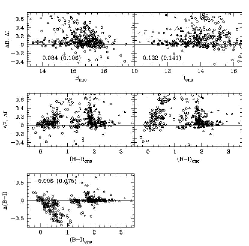
Figure 1: Residuals (in the sense of CFHT minus CTIO) from the comparison of photometry in the cluster core. Also included are the median residual values and in parentheses the semi-interquartile range (a measure of dispersion). Known RR Lyrae stars have been eliminated from the plot. RGB stars are plotted with $\triangle$, AGB stars are plotted with $\Box$, and HB stars are plotted with $\circ$.

In order to collect a nearly complete sample of bright evolved stars in M5, we used data from a variety of sources. The primary source of ground-based photometry was the study of Sandquist et al. (1996; hereafter S96). That dataset was composed of $BVI$ photometry taken at the Cerro Tololo Interamerican Observatory (CTIO) 4 m telescope and $BI$ images of the cluster core taken using the High Resolution Camera (HRCam) on the 3.5 m Canada-France-Hawaii Telescope (CFHT). The CFHT data were obtained during very good seeing conditions so that there was little ambiguity as to the population identifications of cluster stars. Since the 1996 study, the CFHT data have been calibrated against the CTIO 4 m data. Fig. 1 presents a comparison of the photometry for the two datasets. Because stars near the core in the CTIO sample are quite likely to be affected by contaminating light from other nearby stars, there is a substantial bias toward brighter magnitudes. However, the lower envelope of values in the upper 4 plots indicates that the best measured stars have small residuals and little or no trend with color.

We have also used Hubble Space Telescope data from the cluster core reported in Piotto et al. (2002). The F439W and F555W bands were calibrated to $B$ and $V$ by that group, and we present a comparison with our CFHT data in the core in Fig. 2. The $B$ magnitudes show evidence of either a linear trend with $B$ or a second-order trend with color. In the course of examining the HST dataset, we found systematic differences in the position of the RGB in color-magnitude diagrams (CMDs) derived from different CCDs of the WFPC2 camera. For this reason, we found that it was more reliable to make population identifications (RGB, HB, or AGB) based on relative position in the CMD for individual chips. Although this reduces the number of stars on the RGB in the CMDs for each chip and makes it harder to determine where the RGB fiducial line is, the selection of AGB stars is generally cleaner. We have also found that the HST tabulation of Piotto et al. apparently missed some stars whose positions fell near where different chips overlapped. Identification numbers for the stars in the HST dataset that are given in our final tables were composed of the four digit ID number from the Piotto listing, with a leading digit identifying the CCD chip used in the measurement (1 = PC, 2-4 = WF2-4).

Positions in HST frames were derived using the IRAF routine METRIC in the STSDAS package, which converts pixel coordinates to sky coordinates, corrects for geometric distortions of individual chips, and puts coordinates from different chips on the same coordinate system. Lists from different datasets were matched by position using the program DAOMASTER (P. B. Stetson, private communication), which determines six-coefficient coordinate transformations. The positions we tabulate are given in arcseconds from the center of the cluster (taken to be $\alpha=15^{h}18^{m}33\fs 8$, $\delta=+2\arcdeg 4\arcmin 58\arcsec$, epoch 2000.0; Harris 1996), with the x position being the $\alpha$ offset and the y position being the $\delta$ offset (positive being higher $\alpha$ and $\delta$).

Proper motion information from Rees (1993) was used to eliminate field stars from the evolved star samples. Overall this did not impact our samples greatly because M5 is quite far from the galactic plane ($b=46\fdg 8$). The biggest impact of the proper motion information was to verify that most stars bluer than the main line of the AGB were field stars. Because the Rees dataset extends well beyond the bounds of the S96 CTIO fields, we have used his photographic data in the outer cluster regions to identify additional stars to include in the sample. Fig. 3 shows a comparison between Rees’ photometry and our CTIO photometry. Overall, the photometry agrees well, with the exception of slight trends with color for the brightest giants in $B$ and the faintest HB stars in $V$. For the RGB and AGB samples, the inclusion of the Rees dataset allows us to determine complete samples from the center of the cluster to well over $10\arcmin$. Because the Rees data do not reach the faintest HB stars, the HB sample is only complete from the core to approximately $8\arcmin$ from the center.

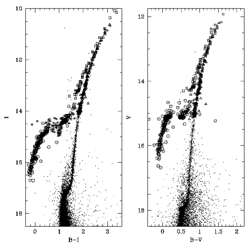
Figure 6: Color-magnitude diagram for stars in the CTIO datasets that are not in the HST or CFHT datasets. The symbols are the same as in Fig. 4. Known RR Lyrae stars are not plotted for the $BV$ dataset.

Although Figs. 2 and 3 make it clear that there are systematic differences in the calibration of the photometry in these different sets, the residuals are less than 0.1 mag in all cases [with the exception of the tip of the RGB in $B$ in the Rees (1993) data] and therefore this is unlikely to make any substantial changes to our conclusions. Johnson & Bolte (1998) indicate that there are some calibration issues in the S96 dataset (mean differences of $\Delta V=-0.039\pm 0.003$ and $\Delta I=-0.021\pm 0.003$, and position-dependent residuals). However, because the offsets for the brightest stars are still only at the level of a few hundredths of a magnitude, and are considerably less serious for stars belonging to the brightest populations (see their Fig. 6), we believe that this is not a serious consideration for this study. Identification of the evolutionary stages of individual stars are made relative to other stars in the same photometric dataset where possible, and there are few cases in which the identification is questionable. The tests of evolutionary theory below are not strongly dependent on the brightness of individual stars because of the samples we have collected are relatively large.

2.1 Population Assignment Criteria

The assignment of a given star into the RGB, HB, or AGB groups was based on position in the CMD. For different regions of the cluster, we used the dataset and color-magnitude combination that provided the cleanest separation of the evolved sequences. The most challenging tasks were distinguishing between upper RGB and AGB stars, and identifying HB stars at all brightness levels with almost no field or cluster star contaminants. In all cases, RGB, HB, and AGB samples were first selected from each individual dataset based solely on CMD position in that dataset. The lists from different datasets were then compared and discrepancies were reconciled, generally in favor of the identification from the highest resolution, least noisy dataset. In each case, we conducted positional searches near the positions of candidates to try and ascertain the reason for the discrepancy (such as blending and CCD flaws).

In the core of the cluster the only practical choices were the HST or CFHT datasets. The CFHT photometry was given higher weight than the HST photometry in regions of overlap because there was smaller amount of scatter in the CFHT photometry on the giant branches. High-resolution photometry of the core of the cluster is important for selecting AGB stars because in lower-resolution ground-based data, blends of RGB and HB stars or two RGB stars can produce objects that appear to be AGB stars. Although this possibility exists in the outskirts of a cluster (meaning that we cannot be certain that our samples are completely free of such blends), the probability of overlap is much smaller.

The stars in the three samples are presented in Tables 1 - 4. The first line for each star contains the new identification number from this study, the offsets from the cluster center in arcsec, and the membership probability (Rees, 1993) when available. Subsequent lines present identifications and photometry from the different catalogs: HST (Piotto et al., 2002), CFHT (S96, calibrated for this study), CTIO (S96, from either the $BV$ or $BI$ calibrations), and PM (Rees, 1993). Notes on some stars are provided in the Table 5. The RGB star sample is truncated at the $V$ magnitude of the HB ($V=15.15$). This falls slightly below the RGB bump.

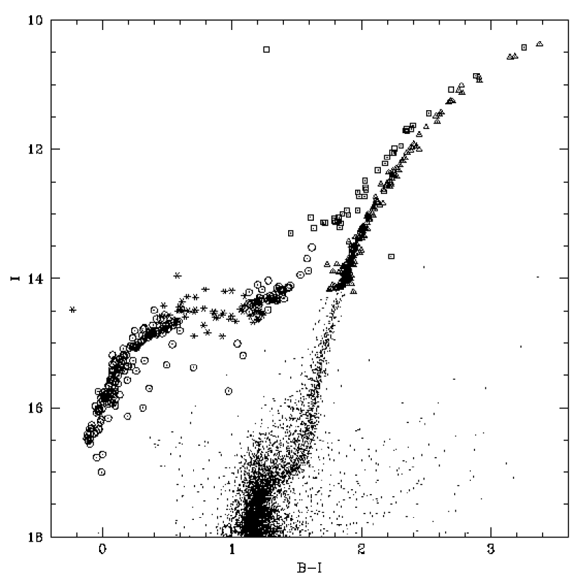
Figure 4: Color-magnitude diagram for the CFHT dataset. Selected RGB stars are plotted with $\triangle$, AGB or post-AGB stars are plotted with $\Box$, HB stars are plotted with $\circ$, and RR Lyrae variables are plotted with $\ast$.

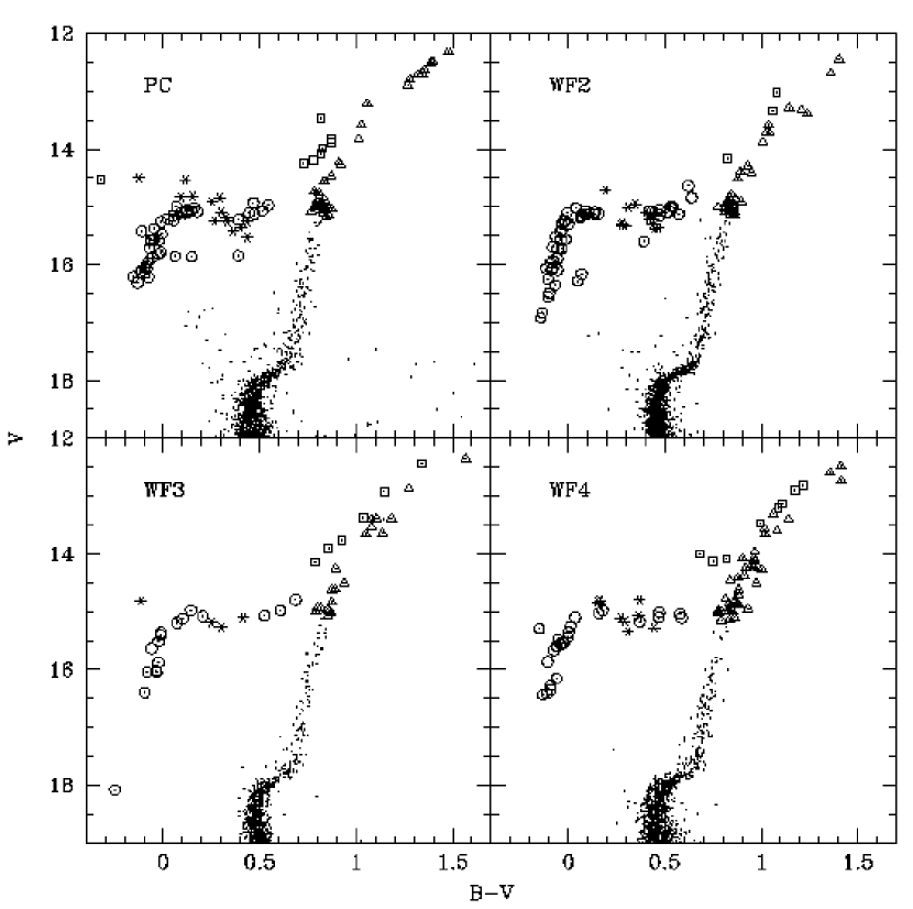
Figure 5: Color-magnitude diagram for the HST dataset (Piotto et al., 2002). The symbols are the same as in Fig. 4.

We also must note a practical aspect to the identification of post-HB stars. We identify AGB stars as being those stars falling close in color to a track nearly paralleling the RGB. Theoretical models predict, however, that stars originating on the bluest portions of the HB never reach the AGB (Dorman et al., 1993). These stars actually spend longer times (up to about 100% longer) in a double fusion shell phase than do AGB stars that come from the reddest portions of the HB, but maintain considerably higher surface temperatures. As a result, proper motion information is important for the separation of these “AGB-manqué” stars from foreground stars that fall in the same portion of the CMD. As can be seen from Figs. 4 and 5, M5 appears to be largely devoid of AGB-manqué stars, which plays a role in its $R_{2}$ value, as we will see in the next section.

When photometry in multiple bandpasses was available, we examined CMDs using different combinations of magnitude and color to help verify identifications. Often the use of the shortest wavelength filter band on the magnitude axis of the CMD was most helpful since this gives both the HB and AGB/RGB a horizontal appearances in the CMD. This can be seen in $U$, $U-V$ CMDs of the cluster (e.g. Fig. 2 of Markov, Spassova, & Baev 2001). CMDs of the different samples are shown in Figs. 4 - 7. We put the CMDs in order of importance in the selection. The CTIO $BI$ dataset is given precedence over the $BV$ dataset due to poorer seeing during the $V$ photometry.

We attempted to identify RR Lyrae variable stars from the literature in order to avoid the accidental elimination of these stars from the HB counts. The primary source of information on these stars was the Catalog of Variable stars in Globular Clusters (hereafter, CVSGC; described in Clement et al. 2001). We have also gathered variability information on RR Lyrae variables for the cluster from Storm, Carney, & Beck (1991; $BV$; intensity-weighted colors), Brocato, Castellani, & Ripepi (1996; $BV$; magnitude averages), Reid (1996; $VI$; magnitude-weighted colors), and Caputo et al. (1999; $BV$; corrected colors). To insure that the resulting “static” colors were on the same scale, we corrected the Storm et al. colors using values from Bono, Caputo, & Stellingwerf (1995). In the process of compiling this list, we discovered that the variables V162 and V163 (Olech et al., 1999) were actually the previously discovered variables V90 and V17 respectively.

3 Diagnostics

3.1 The HB Distribution

3.1.1 HB Observed Color Distribution

HB stars represent the sample from which the AGB stars are born and we observationally identify the portions of the HB that contribute the most stars to the observed AGB by examining the distribution of HB stars. A detailed analysis of this question will require comparison of observations with Monte Carlo simulations of HB and AGB populations using new tabulations of theoretical models with updated compositions and physics. For the time being, we restrict ourselves to characterizing the HB population.

Numerous previous studies have computed HB star distributions where the independent variable is a CMD length coordinate running from the red end of the HB to the blue end (e.g., Crocker, Rood, & O’Connell 1988; Fusi Pecci et al. 1993). Computer implementations of this idea have generally used scale factors to set the relative contributions of increments in color and in magnitude. Ideally though, we would like to be able to relate the derived distribution function to the distribution of HB star masses in a straightforward manner. Although this transformation is complicated by evolution of the stars and uncertainties in chemical composition, these uncertainties mostly affect the average HB mass that is derived, and not the shape of the distribution (Crocker et al., 1988). Because position on the HB is a nonlinear function of total mass, we decided to attempt to remove this nonlinearity using the procedure of Crocker et al. (1988), projecting the stars onto a theoretical ZAHB locus for an appropriate chemical composition. This has the advantage of producing a distribution that will have some physical meaning (something which cannot as easily be said about $\ell_{HB}$ distributions that use fixed color and magnitude scale factors).

We elected to use our $B$ and $I$ photometry in computing mass distributions because the $BI$ datasets cover the vast majority of the stars, have the greatest photometric accuracy, and the $(B-I)$ color is sensitive to temperature over the full range covered by M5 HB stars. We have incorporated RR Lyrae variables using “static” colors derived from studies listed in §2. Since these studies did not use $(B-I)$ colors, we used our CTIO datasets to do a linear interpolation across the instability strip to convert from $(B-V)$ or $(V-I)$ colors to $(B-I)$. For the color distribution shown in Fig. 8, we scaled the RRab and RRc portions of the histogram separately (by 1.771 and 1.38, respectively) to account for known variables (CVSGC) of the two types that do not have measured static colors. For the mass distributions computed below, we randomly chose a $(B-I)$ color from within the range covered by variables with the same pulsation mode ($0.82\lesssim(B-I)\lesssim 1.06$ for RRab variables, and $0.46\lesssim(B-I)\lesssim 0.8$ for RRc variables) if the variable did not have a tabulated static color. The pulsation mode was taken from the CVSGC tabulation. Because the RR Lyrae instability strip covers a relatively small range of mass in the theoretical models ($\sim 0.01M_{\odot}$), the exact method used is not critical to the overall shape of the distribution.

3.1.2 HB Mass Distribution

We plot computed HB mass distributions in Fig. 9 using ZAHB models from VandenBerg et al. (2000) for enhanced $\alpha$-element abundances using two [Fe/H] values roughly corresponding to tabulated values from Zinn & West (1984) and Carretta & Gratton (1997) and a reddening E$(B-I)=0.086$ (Schlegel, Finkbeiner, & Davis 1998). We note that with this reddening the blue tail of the HB observations are not a good color match to the models. Partly the discrepancy seems to result from calibration errors for the CFHT data at the blue end of the HB. This should not be an issue for the mass distributions because the distributions are derived from projections to the ZAHB. For [Fe/H] $=-1.41$, we find $\langle M_{HB}\rangle=0.614$ with $\sigma_{M}=0.031$, while for [Fe/H] $=-1.14$, we find $\langle M_{HB}\rangle=0.591$ with $\sigma_{M}=0.021$. The $\sigma_{M}$ values are somewhat misleading though because the distributions are asymmetric.

The identification of the portion of the HB containing the peak of the mass distribution and the majority of stars is a robust result of this procedure, independent of the exact values of the star masses. The peak of the distribution falls at $(B-I)_{peak}=0.50$ (right at the blue edge of the instability strip), while the median color value is $(B-I)_{med}=0.43$. We can characterize the width of the HB color distribution in several ways as well. From looking at the HB mass distribution, and identifying by eye where the distribution drops off most quickly, we can crudely bracket the range of colors containing the majority of stars. In this way, we find that the red edge of the mass distribution at $(B-I)=1.05$ (essentially the red end of the instability strip), and the blue edge falls on the blue tail at $I\approx 16.2$ (although this is more poorly defined). The stars on the red side of the instability strip form a tail in the mass distribution largely because HB color changes much more slowly with mass there. Alternately we can identify the middle 68.3% of the HB sample (corresponding to $1\sigma$ points of a Gaussian distribution). In this way we find a red bound at $(B-I)=1.14$ in the blue half of the constant red HB, and a blue bound at $I\approx 15.8$ on the blue tail. These two methods give similar results.

3.1.3 Oosterhoff Group Considerations

The color distribution emphasizes a peculiar property of M5: a majority of M5’s HB stars fall on the nonvariable blue HB, but M5 is an Oosterhoff group I cluster with the expected excess of RRab type variables ($N_{c}/N_{ab}=39/91=0.43$; CVSGC), which reside on the red side of the instability strip. In fact, M5 has one of the bluest HBs of the Oosterhoff group I clusters in the Galaxy. Recently Jurcsik et al. (2003) presented evidence that the dominant Oo I population in M3 is composed of stars in the early stages of post-ZAHB evolution, and that stars that have begun to evolve redward appear to have an Oo II-like population. Jurcsik et al. reference the hysteresis hypothesis of van Albada & Baker (1971) that proposed that switches between fundamental and overtone pulsation modes occur at different temperatures depending on the direction of the star’s evolution in color. This may also be the case for M5: its Oo I variable population derives from the fact that the ZAHB in the instability strip is populated as a result of the cluster’s large dispersion in $M_{HB}$. However, this does not explain why the distribution of static colors for the variables is biased toward the red half of the instability strip. M5 is one of the only Oo I clusters for which the number of stars per color interval should be rising as you go from the red end of the instability strip to the blue end, but the cluster still has many fewer RRc variables than RRab variables. Theoretical evolution tracks do not diverge from this portion of the HB toward the red and blue. This seems to imply that HB stars are being kept out of the range of colors that are normally occupied by RRc variables. In other words, the presence of pulsation seems to affect the evolutionary track of the star.

Our discussion has focussed on published values of static colors; however, there is no reason to believe that this affects the conclusion. The larger number of fundamental mode pulsators is undeniable, and the vast majority of those RR Lyrae stars having static colors fall in two distinct color ranges sorted by the pulsation mode. The fraction of variables pulsating in the first overtone in other globular clusters also shows very little dependence on HB morphology (e.g. Castellani, Caputo, & Castellani 2003).

3.1.4 Unusual HB Stars

In order to facilitate the identification of unusual stars, we plot a CMD for the combination of the CFHT and CTIO datasets in Fig. 12. This is the largest sample with a common photometric calibration (although a slight mismatch in the colors of the bluest HB stars in the two datasets is evident).

In examining HB stars, we have found several groups of stars with unusual magnitudes and colors even in the best datasets. There are two separate groupings of stars redder and brighter than the most populated portion of the red HB in M5. These two groups may correspond to groups in M3 that were given the classification “ER” by Ferraro et al. (1997). The brighter of the two groups ($I<14$) contains 11 stars (IDs 13, 28, 30, 53, 110, 118, 137, 141, 168, 239, 392) and is at the extreme red end of the HB, noticeably disconnected from the rest of the HB. The fainter of the two groups ($14.08<I<14.28$; see Fig. 10) is less noticeably separated from the red HB and contains 14 stars (IDs 34, 42, 62, 63, 67, 76, 169, 198, 360, 389, 412, 425, 434, 444). The two groups contain about 4.5% of the total HB sample.

Fusi Pecci et al. (1992) hypothesized that the ER HB stars are the progeny of blue straggler stars — because blue stragglers are believed to have mass larger than turnoff mass stars, when they evolve to the core He fusion phase, they would tend to have higher masses and redder colors than the majority of HB stars. Ferraro et al. (1997b) provide some evidence that the radial distribution of ER stars in M3 parallels that of the stragglers. Ferraro et al. (1999) find than the cumulative radial distribution of the ER HB stars parallels that of the blue stragglers, and both are more centrally concentrated than the combined RGB and HB sample. For M5, we find that the cumulative radial distribution of the two groups of ER HB stars is actually less concentrated than the HB stars (Fig. 11). From a Kolmogorov-Smirnov test, there is only a probability of 0.0014 that the two samples come from the same distribution. (The redder of the two groups of ER HB stars is too small to make a statistically significant comparison.) However, 10 of these stars are concentrated of these stars within about $1\arcmin$ of the edge of the high resolution HST and CFHT fields, so that there is a good chance some of these are unresolved blends of an HB and an RGB star. While blends are unlikely to explain other identified ER HB stars (particularly when the ones forming a tight group in the CMD), higher resolution photometry of the near-core region is needed.

We have also identified 13 stars fainter than the horizontal portion of the HB and redder than the blue tail (see Fig. 10). All of these stars are found within $100\arcsec$ of the core. As with the ER stars, several (IDs 81, 95, 302, 317) are found just outside the HST and CFHT fields, and so may be blends of a blue HB star and a star on the faint half of the RGB. Others (IDs 177, 243, 316) are found near the cluster core and were only measured in the CFHT field, so that they may also be blends. However, others (IDs 107, 201, 221, 250, 268, 276) were measured in both the HST and CFHT fields, and deviate in similar ways in both datasets. Blends or unresolved binaries involving a blue HB star and a star on the lower RGB are one possibility. In a few of the cases, it is also possible that the stars are extremely bright blue stragglers. A less likely possibility for a subset of these stars (IDs 268 and 317) is that there may be unidentified RR Lyrae stars caught in a particular part of the pulsation cycle.

Two stars are found in the RR Lyrae instability strip in different datsets. HB star 340 falls within the instability strip in the HST dataset, and within the area of the CMD covered by RR Lyrae stars measured in the CFHT datset. As a result, we flag it as possible RR Lyrae star. Star 132 is relatively near the core, but falls within the instability strip in the CTIO dataset. It may be a blend of an blue HB star and and giant star.

Finally we note that there is one star in the HST and CFHT datasets (ID 341) several magnitudes below the blue end of the HB that may be an extreme blue HB star. In spite of the fact that it is observed in the core of the cluster, it may still be a field star, or a cluster member in an evolutionary phase following the AGB. The star is substantially bluer than the main sequence in both the $B-V$ and $B-I$ colors. We cannot distinguish between these possibilities with the datasets discussed here.

3.2 The Population Ratio $R_{2}$

3.2.1 Theory

The population ratio $R_{2}=N_{AGB}/N_{HB}$ is a diagnostic of the relative durations of the helium fusion phases of stellar evolution (Buzzoni et al. 1983). As discussed by several groups (e.g. Straniero et al. 2003; Renzini & Fusi Pecci 1988), this ratio is most affected by the physical processes occurring in the cores of stars during the horizontal branch (HB) phase. The largest uncertainties in theoretical predictions for this ratio are the rate for the ${}^{12}\mbox{C}(\alpha,\gamma)^{16}\mbox{O}$ reaction and details of the mixing processes occurring at the outer boundary of the convective core. Even with these uncertainties, observed values of $R_{2}$ are sufficient to rule out the possibility of the so-called “breathing pulses” seen in early models of AGB stars. Breathing pulses mix fresh helium into the core and hence prolong the HB phase, resulting in low $R_{2}$ values. As a result of $R_{2}$ measurements, ad hoc algorithms have been introduced into the models to suppress these pulses (e.g. Cassisi et al. 2001).

There are observational influences on the $R_{2}$ ratio that have been mostly ignored up to this point. Typically, a HB star becomes brighter and redder as it evolves toward the AGB (although the star may make smaller excursions blueward and redward in color before leaving the HB entirely). Theoretical models (e.g. Dorman, Rood, & O’Connell 1993) showed that stars evolving off of the bluest extensions of a HB may turn blueward before they reach the portions of the CMD most heavily populated by AGB stars. Generally only stars less massive than about $0.53M_{\odot}$ will completely avoid the AGB, although the exact value depends on chemical composition. Slightly redder HB stars reach the upper AGB, but turn off toward the white dwarf cooling sequence before reaching the tip of the AGB. HB stars that are slightly redder still start the AGB phase in the AGB clump, which results in a large increase in AGB lifetime. Clearly the HB morphology of a globular cluster will affect the number of AGB stars that are present.

An important point of this discussion is that “second parameter” effects on the HB morphology can cause differences in the $R_{2}$ ratio for globular clusters of the same metallicity. As illustrations, we present sample single-star $R_{2}$ values calculated from the models of Dorman, Rood, & O’Connell (1993) in Fig. 13. We should keep in mind that the Dorman et al. models have physical inputs that are somewhat out of date: oxygen-enhanced compositions (rather than $\alpha$-element enhanced), a somewhat low initial $M_{core}$ [compared to Catelan et al. (1998), for example], and potentially an initial envelope helium abundance $Y_{env}$ that is not consistent with other observational constraints (Sweigart & Catelan, 1998). However, the general features of this figure should not change. This leads to at least two interesting questions. First, is it possible to observe differences between the AGB populations of clusters whose HB stars show second parameter effects? Second, is it possible to predict a cluster’s $R_{2}$ value given its metallicity and particular HB morphology, or does the second parameter affect the AGB as well?

3.2.2 Observations

From our dataset, we find $N_{AGB}=98$ and $N_{HB}=557$ for the total sample, excluding stars found only in the Rees (1993) dataset. Thus, we have $R_{2}=0.176\pm 0.018$, where the error is computed using

$$\sigma^{2}(R_{2})=R_{2}/N_{HB}.$$

This error formula was derived under the assumption that stars that have passed the He flash can only have two identifications (HB or AGB), and therefore are described by the binomial distribution with the probability of being in the AGB phase $p=N_{AGB}/(N_{HB}+N_{AGB})=R_{2}/(1+R_{2})$. The resulting error $\sigma^{2}(R_{2})$ is smaller than what is derived from Poisson errors by a factor of $(1+R_{2})^{-1}$. The large samples of stars have allowed us to substantially reduce the error on the determination.

The maximum single-star $R_{2}$ values from Dorman et al. (1993) do agree with the observed value for M5. However, more recent models by Cassisi et al. (2003) with updated ${}^{12}\mbox{C}(\alpha,\gamma)^{16}\mbox{O}$ rate and equation of state produce a value $R_{2}=0.12$, significantly lower than the Dorman et al. (1993) and Cassisi et al. (2001) models. The newer theoretical results are out of agreement with the $R_{2}$ value for M5 by more than $3\sigma$, although they are in better agreement with values from the majority of clusters with reasonably large measured samples. In the tabulation of Sandquist (2000), there were 8 clusters with more than 200 measured HB stars (see Fig. 14). Excluding M5, we compute $\langle R_{2}\rangle=0.106\pm 0.038$. For the four clusters with redder HB morphologies than M5, $\langle R_{2}\rangle=0.106\pm 0.011$. So, while the most recent theoretical models are in agreement with values from the globular clusters with the largest tabulated samples, M5 has a value that appears to be out of agreement with other clusters and with the theoretical values. In fact, the $R_{2}$ value is one of the highest seen for a globular cluster to date. That M5 has a high $R_{2}$ value has been apparent even in smaller subsamples (see Table 7 of S96).

The effect that HB morphology has on numbers of AGB stars can be crudely seen using the ratio $R_{HB}=(B-R)/(B+V+R)$ (Lee, Demarque, & Zinn 1994), where $B$, $V$, and $R$ are numbers of blue, variable, and red HB stars. M5 has $R_{HB}=0.37$ (this paper), while the slightly more metal-poor cluster M3 has $R_{HB}=0.19$. A preliminary determination of $R_{2}$ for M3 gives a value of $0.136\pm 0.016$. Overall M3 has a redder HB morphology than the more metal-rich M5, and has an $R_{2}$ value that is more consistent with typical theoretical predictions. However, the differences in $R_{2}$ values are not necessarily as simple as a shift in the peak color of the HB distribution because the color distributions of the two clusters overlap to a large extent. In addition, the competing effects of HB morphology and metallicity mean that the masses of HB stars in these two clusters are likely to be similar. (Higher metallicity makes the ZAHB mass at a given color smaller, while a bluer HB morphology at a given metallicity generally means a lower mean HB mass.) Catelan (2000) computed synthetic HBs for M5, and found that a mean mass $\langle M_{HB}\rangle=0.633M_{\odot}$ and a mass dispersion $\sigma_{M}=0.025M_{\odot}$. In a similar study for M3, Catelan et al. (2002) finds $\langle M_{HB}\rangle\approx 0.64M_{\odot}$ and $\sigma_{M}\approx 0.02M_{\odot}$ (although they state that there appears to be a systematic difference in $\langle M_{HB}\rangle$ as a function of cluster radius). So although the mean mass and mass dispersion for M3 and M5 appear to be similar, M5 has a bluer HB and more AGB stars.

3.2.3 N_AGB/N_RGB

Theoretical models predict that the bluest HB stars that reach the AGB spend a somewhat longer time in the AGB phase (Cassisi et al., 2001) than redder HB stars due to smaller envelope mass and weaker fusion shell sources. [This last point was mentioned briefly by Dorman & Rood (1993).] Models indicate that the stars with maximal AGB lifetimes originate on the blue tail of the HB, where the HB luminosity has dropped by about a factor of 2 from what it is in the instability strip. As a result, there should also be an enhancement of the numbers of AGB stars relative to numbers of stars in other phases of evolution. Using the numbers of RGB stars tabulated in Sandquist (2000), we examine in Fig. 14 the population ratio $R_{1}=N_{AGB}/N_{RGB}$, where $N_{RGB}$ is the number of RGB stars more luminous than the HB. The relative positions of the clusters in a plot of $R_{1}$ versus $R_{HB}$ do not change — M5 still has a higher value than clusters with redder morphologies, which supports the idea that M5 stars spend longer times in the AGB phase than those in clusters with redder HB morphologies. This indicates that M5 may be anomalous in some way, which would mean that input physics for the stellar models is not the reason for the difference.

We note that the two clusters with the most extended blue HBs (NGC 2808 and NGC 6752) have $R_{2}$ $<0.1$, consistent with the idea that a significant fraction of the stars are avoiding the AGB phase. The cluster M30 also has a low $R_{2}$ value, but a much more compact blue HB. M30’s metallicity is low, however, which makes it more likely that some of its bluest HB stars would also miss the AGB (see Fig. 13). The cluster M55 stands out as having high $R_{1}$ and $R_{2}$ values that are similar to those found for M5. Overall, M55 has a compact blue HB with the HB distribution peaking near the bright end of the blue tail. It also has a considerably lower metallicity than M5, which probably means that the change in HB track morphology will occur at higher temperatures as well. This should be checked with a study using synthetic HB and AGB populations.

Unfortunately, there are no sets of HB and AGB star models tabulated in the literature for the most recent physical inputs. As a result we are unable to gauge the exact effect of the HB morphology of M5 on the $R_{2}$ value. If the Dorman et al. (1993) models are any guide, then the $R_{2}$ value would be increased if the majority of the HB stars have masses giving them proportionately long AGB phases. The large $R_{2}$ value found for M5 indicates that only a small fraction of the observed HB stars are likely to avoid having an AGB phase, which makes it possible to place a color constraint on where the morphology of the post-HB evolutionary tracks change. Stars that do not reach the AGB still spend a large amount of time brighter than the HB and bluer than the AGB. Because we have found no cluster members significantly to the blue of the heavily-populated AGB, the post-HB evolutionary tracks are not likely to change until $I\gtrsim 16.4$, at the observed tip of M5’s HB. In addition, because the time spent on the AGB changes rapidly with decreasing mass, it might be possible in the future to calibrate HB star masses using this feature. It may also be possible to empirically determine which HB stars have the maximum relative AGB lifetime $t_{AGB}/t_{HB}$.

The examination of large AGB star samples gives us a way of testing the morphology of HB tracks to see whether stars from the most populated portions of the HB really do reach the AGB and whether they spend the predicted amount of time there (relative to the time spent on the HB). By examining clusters with bluer HB morphologies or lower metallicity, we can attempt to empirically identify the point on the HB at which the stars no longer have an AGB phase. Although there should be smaller differences in $R_{2}$ values between clusters with red HBs and those with intermediate morphologies, it may also be possible to identify those stars which have AGB phases of maximum duration.

3.3 The Luminosity Functions and Evolutionary Timescales

The luminosity function (LF) of red giant branch stars is sometimes used to test theoretical predictions for evolution timescales of evolved stars. Although with AGB stars we are dealing with smaller samples than are available for RGB stars, we can extract evolutionary information using the cumulative LF. It is well-known that the logarithm of the cumulative LF for stars on the upper RGB is linear with magnitude (Fusi Pecci et al., 1990). The structure of AGB stars is similar to that of RGB stars with the hydrogen fusion shell providing the majority of the luminosity during most of the evolution. We examined the models of Dorman et al. (1993) and found nearly linear relationships between $\log(t_{tAGB}-t)$ and $\log(L/L_{\odot})$ for AGB evolution between the luminosity minimum in the AGB clump and the luminosity maximum before the first thermal pulse. ($t_{tAGB}$ is the age of the star at the luminosity maximum.) In addition, the slope of the relation is nearly identical for stars of very different mass, and is also fairly insensitive to metallicity. The situation is somewhat complicated by the AGB clump (see §3.4 below) and by thermal pulses (involving interactions between the He and H fusion shells), but if we restrict ourselves to AGB stars brighter than the clump, the logarithm of the cumulative LF should also be linear with magnitude. Because thermal pulses last a very small portion of the total AGB evolution (10% or less), they can be safely neglected here.

For cool stars, magnitudes derived from redder filter bands are most linearly related to $\log(L/L_{\odot})$. For our RGB and AGB samples we have selected the best $I$ photometry for each star. We have chosen from the CFHT dataset where available, and from the CTIO data in all other cases (except for stars outside the CTIO field for which no $I$ photometry was available). These two sets have the least scatter in the respective CMDs and are also very nearly on the same photometric system.

The cumulative LF in $I$-band for M5 is presented in Fig. 15. There are two features in this figure that we wish to discuss: the behavior of the RGB LF at the bright end, and the slopes of the RGB and AGB LFs. In the figure we compare with theoretical LFs for the RGB from Kim et al. (2002; hereafter, Y² models) for two different color-$T_{\mbox{eff}}$ transformations. The distance modulus used in these comparisons was $(m-M)_{I}=14.36$ (S96). While the models reproduce the observed magnitude difference between the RGB tip and the RGB bump to within 0.1 mag and the slope of the cumulative LF immediately brighter than the bump ($12<I<13.9$), there appear to be too few stars observed near the red giant tip. Systematic errors in the color transformations or underestimation of the neutrino emission rates used in the stellar models (e.g. Haft, Raffelt, & Weiss 1994) might be able to account for at least part of the difference. [Changes to neutrino emission rates have other consequences, however: more than a 50% change to the rates would result in greater than a 0.1 mag increase in the brightness of the RGB tip, which would probably be inconsistent with the observations (Raffelt & Weiss 1992).] It should be kept in mind that identification of RGB and AGB stars becomes most uncertain near the tip of the RGB where the two branches are closest together in color. However, the number of “missing” RGB stars appears to be about 8, which is as much as 50% of the predicted sample at $I<10.8$. Small horizontal shifts in magnitude do not affect this discrepancy noticeably. If we use models with [Fe/H] corresponding to the Zinn & West (1984) scale, the models which match the magnitude level of the RGB bump also fit most of the upper RGB well, and the slope of the RGB in the CMD is a closer match to the observations. However, the fit is unsatisfactory because the tip of the RGB is too faint by 0.4 mag (9 observed stars fall above the theoretical prediction), and it requires a distance modulus $(m-M)_{I}\approx 14.85$ (well outside the range determined from subdwarf fitting to the main sequence).

To gauge the significance of this difference, we conducted Monte Carlo simulations. In each trial we randomly chose 300 stars (the number of observed stars with $I<13.9$) from a cumulative probability distribution derived from the theoretical cumulative LF from Y² models (with Green et al. 1987 color-$T_{\mbox{eff}}$ transformations). We then measured the largest difference in $\log N$ between the simulated and theoretical values at the $I$ magnitude of each simulated star. The largest deviations in number $N$ tend to occur near the faint limit of the sample, but the largest fractional differences (or differences in $\log N$) occur closest to the tip in the simulations. Even so, in a run of 100,000 trials, we found 1168 trials with $\log(N_{theory}/N_{sim})>0.5$. (The rms value was 0.199.) If we look for trials having $\log(N_{theory}/N_{sim})>0.3$ at $I>10.7$, we found 1849 trials of 100,000 meeting the conditions. As a result, the low number of RGB tip stars observed in M5 is marginally significant, with a probability of less than 2% of being due to statistical fluctuations. In view of the importance to the understanding of the physics of the upper RGB, other well-populated clusters should be examined.

The fitted slopes of the AGB and RGB cumulative LFs are significantly different: $0.3458\pm 0.0015$ for the RGB above the bump ($12<I<13.9$), and $0.496\pm 0.015$ for the AGB ($I<12.8$). The shorter evolutionary timescale for AGB stars is responsible for differences in the total numbers of stars, but the slope relates to the change in the evolutionary timescale as the brightness changes. The RGB slope agrees closely with predictions from stellar models

$$\frac{d\log\Phi_{RGB}}{dM_{I}}\approx\frac{d\log(t_{tRGB}-t)}{d\log L}\frac{d\log L}{dM_{I}}\approx-0.9/-2.5=0.36,$$

where $\Phi_{RGB}$ is the cumulative luminosity function for RGB stars. The comparison with predictions for the AGB is somewhat more complicated because the slope has a slight dependence on star mass, with the slope being minimum for the bluest HB stars that have an AGB phase. From Dorman et al. (1993) models, the predicted slope is still too high:

$$d\log\Phi_{AGB}/dM_{I}\approx-1.33/-2.5=0.53,$$

where $\Phi_{AGB}$ is the cumulative luminosity functions for AGB stars.

To test whether the difference between the observed and predicted values for the slope of the AGB cumulative LF is significant, we conducted additional Monte Carlo simulations. We ran 50,000 trials selecting 48 stars (the number of AGB stars in M5 that were fit to determine the slope) from a cumulative probability distribution having a slope $d\log P/dI=0.53$, and determined an observed slope from each simulated sample. The trials (see Fig. 16) indicate that there is a significant bias toward measuring a shallower slope (the average was 0.489, and the mode was 0.47), and the HWHM of the distribution of slopes was 0.09. The bias comes from stars at the bright end, which are given somewhat more weight due to the nature of the cumulative LF: the stars are less abundant, and contribute at a place in the LF where the addition of a star makes a large fractional change.

Based on the simulations, our observed slope is quite consistent with the theoretical prediction, and is in fact almost exactly what is expected when the bias in measurement is factored in. However, the simulations indicate that the cumulative LFs are not likely to be able to give us a strong constraint on AGB evolution in a practical sense. Fig. 16 shows the distribution of results for Monte Carlo trials involving 100 stars on the upper part of the AGB. The mode of the distribution (0.50) is closer to the input value (0.53), and the HWHM of the distribution is smaller (0.06). However, there are only a handful of clusters in the Milky Way that have large enough populations of bright AGB stars.

3.4 The AGB Clump

With the large AGB sample, we can introduce new diagnostics to test our understanding of the physics affecting the evolution of these stars. The AGB phase is characterized by the progression of a helium fusion shell source through a helium profile set up during the HB phase. As discussed by Renzini & Fusi Pecci (1988), this means than the distribution of stars on the AGB is a reflection of the helium abundance of the gas being consumed by the shell. The spatial resolution of the helium fusion shell as a probe of the chemical profile is poorer than the resolution of the hydrogen fusion shell during the first ascent of the giant branch because the helium shell is thicker. The red giant branch (RGB) bump in globular clusters provides us with a way of measuring the depth to which the convective envelope reaches. A similar feature appears at the base of the AGB, called the “AGB clump”. During HB evolution, the action of semiconvective mixing leaves a region of changing helium abundance that the helium fusion shell processes at the beginning of the AGB phase. While this happens and the shell stabilizes with the nearly pure helium mixture outside the mixed region, an AGB star remains in the clump.

Ferraro et al. (1999) discuss a magnitude difference diagnostic involving the AGB clump. $\Delta V^{HB}_{AGB}=V^{AGB}_{clump}-V_{ZAHB}$ is defined in analogy to a more widely used indicator for the RGB bump: $\Delta V^{bump}_{HB}=V^{RGB}_{bump}-V_{ZAHB}$. Ferraro et al. found good agreement with theoretical models using the FRANEC code (Straniero, Chieffi, & Limongi, 1997) for nine globular clusters, although this required careful simulation of the HB and determination of the level of the ZAHB. Because there are no recent sets of HB/AGB models available, we will not discuss this indicator further here. In addition, a earlier comparison of the theoretically predicted colors of AGB clump stars with observations indicated that the theoretical predictions were too blue (see Fig. 25 of S96). Again though, this kind of comparison is somewhat sensitive to composition and color-$T_{eff}$ transformations, and so we have chosen not to discuss this here.

The number of stars found in the clump is related to the richness of the helium in what was the outer convective core. To attempt to test the evolution of the clump stars, we introduce a new diagnostic $R_{clump}=N_{clump}/N_{AGB}$, where $N_{clump}$ is the number of stars in the AGB clump (between the base of the clump and a point 0.25 $V$ magnitudes brighter). Such a definition avoids the need to attempt to identify the upper boundary of the clump in the AGB samples we gather. The 0.25 mag size is approximately what is predicted theoretically for the height of the clump, however.

The base of the AGB clump can be identified using the cumulative LF presented in §3.3. The base of the AGB clump seems to fall at $V=14.20$ in the CTIO dataset. There are a small number of stars fainter than this, but which appear to be better classified as AGB stars than HB stars. We include these stars in the “clump” category, and find $N_{clump}=45$, $N_{AGB}=103$, and $R_{clump}=0.44\pm 0.05$. We have used

$$\sigma^{2}(R_{clump})=\left(\frac{R_{clump}}{1+R_{clump}}\right)N_{AGB}^{-1}.$$

To make a more direct connection with theoretical models, we also create a similar operational definition for $I$-band photometry: stars within 0.30 mag of the base of the AGB clump. We find that the base of the clump is at $I=13.25$ in the M5 data, and using this we get $N_{clump}=41$, $N_{AGB}=99$, and $R_{clump}=0.41\pm 0.05$ since the outermost AGB stars do not have $I$ photometry.

From the models of Dorman et al. (1993) shown in Fig. 13, we see a couple of useful features of this indicator: it is roughly constant with HB mass for $M\gtrsim 0.56M_{\odot}$, and the values for the two most metal-rich compositions tabulated are quite similar: $R_{clump}\approx 0.55$. From this comparison, we find that the observed value for M5 is a little over $2\sigma$ too low compared to theory. Once again, we must remind the reader that the Dorman et al. (1993) models have somewhat dated physical inputs that may result in some systematic errors. Until updated models are publicly available, we merely point out areas where it may be possible to learn new details about the stellar interiors.

As a final note, the models of Cassisi et al. (2001) indicate that the inclusion of breathing pulses in theoretical models decreases the AGB lifetime by more than 25%, primarily by considerably shortening the time spent in the clump. Our results for $R_{2}$ and $R_{clump}$ add more support for the idea that breathing pulses should somehow be suppressed in models of HB stars.

4 Conclusions

We have compiled a nearly complete list of bright RGB, HB, and AGB stars for the globular cluster M5 reaching from the core of the cluster to $8-10\arcmin$ from the center. We have used these samples to conduct a thorough comparison with theory in order to test stellar interior physics under the conditions prevalent in these bright stars. We have introduced a new diagnostic $R_{clump}$ for evaluating the evolutionary timescale in the early part of the AGB phase, finding that there is a marginal disagreement between the observations and the models of Dorman et al. (1993). On the whole we find good agreement between observations and theory for the cumulative LFs of the RGB above the RGB bump and for the AGB, indicating that the evolutionary timescales in both phases are predicted accurately. An apparent exception appears near the tip of the RGB, where there appear to be too few giants compared to theoretical predictions. The chance that this is a statistical fluctuation is less than 2%. This may be an indication that the neutrino emission rates in the cores of these bright stars are underestimated.

The most significant result is the large value for the population ratio $R_{2}$ compared to recent theoretical values. The high value is probably the result of the particular HB morphology of the cluster and not continuing uncertainties in physical inputs like the cross section for the ${}^{12}\mbox{C}(\alpha,\gamma)^{16}\mbox{O}$ reaction or the core mixing algorithm. We encourage new calculations of HB and AGB phases using updated physics because AGB stars provide a means of testing predictions for the morphology of evolutionary tracks for stars fusing He into C and O and of constraining the ${}^{12}\mbox{C}(\alpha,\gamma)^{16}\mbox{O}$ reaction rate. In particular, they stand the greatest chance of identifying the color at which HB stars change from going into or not going into a typical AGB phase, and the range of colors for which the AGB phase has its maximum duration.

We also call attention to a peculiarity of the distribution of stars on M5’s HB. We find that the mass distribution for HB stars peaks at a position corresponding to the blue edge of the instability strip. The instability strip is heavily populated due to the large dispersion in HB masses ($0.02-0.03M_{\odot}$). However, the distribution of stars within the instability strip is heavily biased toward the red half of the instability strip. This is consistent with M5 being an Oosterhoff group I cluster, but it means that the first overtone instability strip is underpopulated compared to the fundamental strip to the red and compared to the nonvariable stars to the blue. Because M5 has one of the bluest HB morphologies of the Oo I clusters (including the more metal-poor M3), it is a severe test of potential explanations of the Oosterhoff dichotomy. Some mechanism for reducing the evolutionary timescale of stars in the first overtone instability strip seems to be needed. The blue half of M5’s instability strip should be more heavily populated — the big question is why it isn’t.

Figure 2: Residuals [in the sense of HST (Piotto et al., 2002) minus CFHT] from the comparison of photometry in the cluster core. Also included are the median residual values and in parentheses the semi-interquartile range (a measure of dispersion). Known RR Lyrae stars have been eliminated from the plot.

Figure 3: Residuals [in the sense of Rees (1993) minus CTIO] from the comparison of photometry in the cluster outskirts. Also included are the median residual values and in parentheses the semi-interquartile range (a measure of dispersion). Known RR Lyrae stars have been eliminated from the plot.

Figure 7: Color-magnitude diagram for the Rees (1993) dataset. The symbols are the same as in Fig. 4.

Figure 8: The distribution of $(B-I)$ colors for M5 HB stars. Known RR Lyrae stars are shown in the shaded part of the histogram.

Figure 9: HB mass distributions computed using $\alpha$-element enhanced models of VandenBerg et al. (2000).

Figure 10: Zoomed CMD for HB stars identifying two groups of extremely red HB stars (ER HB) and stars likely to be unresolved blends of blue HB stars and faint RGB stars.

Figure 11: Cumulative radial distributions of RGB (dotted line), HB (solid line), AGB (dashed line), and extreme red HB (thick solid line) stars.

Figure 12: Combined color-magnitude diagram for stars in the CFHT and CTIO datasets. Stars measured in both datasets are plotted with photometric values from the CFHT dataset. The symbols are the same as in Fig. 4.

Figure 13: Timescale ratios involving AGB phases from the oxygen-enhanced models of Dorman et al. (1993). Upper panel: ratio of durations of the AGB and HB as a function of star mass. Bottom panel: ratio of the durations of the AGB clump phase and the total AGB phase.

Figure 14: Population ratios for globular clusters having more than 200 HB stars in the tabulation of Sandquist (2000). $R_{HB}$ values come from the tabulation of Lee et al. (1994). From left the right the clusters are: 47 Tuc, NGC 2808, NGC 1851, M3, M5, M53, M30, M55, and NGC 6752.

Figure 15: Cumulative luminosity functions for AGB thick solid line and RGB thick dotted line stars. The two curves with thin lines are theoretical predictions from Y² models (Kim et al., 2002) for [Fe/H] $=-1.11$ and age 12 Gyr with color transformations from Green et al. (1987; solid line) and Lejeune et al. (1998; dashed line). Also shown are linear fits to the AGB ($I<12.8$) and RGB ($12<I<13.9$).

Figure 16: Results of Monte Carlo simulations of the slope of the cumulative luminosity function of bright AGB populations for 48 and 100 stars.

Table 1: The AGB Star Sample for M5

ID	$\Delta\alpha(\arcsec)$	$\Delta\delta(\arcsec)$	$P_{\mu}$	Alternate ID
	ID		$B$	$V$	$I$	Catalog
1	$-135.209$	$-125.364$	0.99	V42
	1		12.81	10.93		PM
2	7.296	$-34.384$
	1		$13.3947\pm 0.0689$		$10.0907\pm 0.1270$	CT
3	6.125	86.957	0.99
	2		$13.5448\pm 0.0054$		$10.1608\pm 0.0730$	CT
			$13.5565\pm 0.0050$	$11.9222\pm 0.0025$		CT
	2		13.98	12.02		PM
4	28.847	$-72.530$
	5		$13.4689\pm 0.0142$		$10.3608\pm 0.1110$	CT
5	7.478	$-34.628$
	6146		$13.6798\pm 0.0040$		$10.4222\pm 0.0015$	CFH
6	35.655	$-42.208$
	6665		$11.7171\pm 0.0189$		$10.4512\pm 0.0094$	CFH
7	$-79.898$	$-28.895$	0.99
	14		$13.6607\pm 0.0086$		$10.7752\pm 0.0740$	CT
			$13.6925\pm 0.0090$	$12.3870\pm 0.0024$		CT
	10		13.87	12.37		PM
8	30.902	$-76.439$
	15		$13.6805\pm 0.0160$		$10.7819\pm 0.0600$	CT
			$13.6789\pm 0.0160$	$12.2595\pm 0.0022$		CT
9	53.961	69.500	0.99
	32456		$13.7817\pm 0.0224$	$12.4399\pm 0.0643$		HST
	603		$13.7703\pm 0.0008$		$11.0759\pm 0.0035$	CFH
	22		$13.6924\pm 0.0079$		$11.0324\pm 0.0310$	CT
			$13.7025\pm 0.0080$	$12.4456\pm 0.0021$		CT
	15		13.90	12.48		PM
10	114.220	61.938	0.99	I-20
	28		$13.8090\pm 0.0058$		$11.1332\pm 0.0280$	CT
			$13.8064\pm 0.0060$	$12.4973\pm 0.0014$		CT
	20		14.02	12.62		PM

Note. — The complete version of this table is in the electronic edition of the Journal. The printed edition contains only a sample.

Table 2: The RGB Star Sample for M5

ID	$\Delta\alpha(\arcsec)$	$\Delta\delta(\arcsec)$	$P_{\mu}$	Alternate ID
	ID		$B$	$V$	$I$	Catalog
1	$-32.782$	$-17.291$
	4873		$13.7470\pm 0.0000$		$10.3694\pm 0.0069$	CFH
	4		$13.7046\pm 0.0190$		$10.3198\pm 0.0530$	CT
			$13.7092\pm 0.0190$	$12.0561\pm 0.0027$		CT
2	33.925	99.017
	32361		$13.9193\pm 0.0242$	$12.3500\pm 0.0217$		HST
	6		$14.0165\pm 0.0044$		$10.3842\pm 0.0980$	CT
			$14.0990\pm 0.0049$	$12.5138\pm 0.0019$		CT
3	15.390	$-44.225$
	6680		$13.7474\pm 0.0000$		$10.5605\pm 0.0044$	CFH
	3		$13.4374\pm 0.0609$		$10.2996\pm 0.1180$	CT
4	$-5.435$	0.678
	210174		$13.7950\pm 0.0210$	$12.3154\pm 0.0395$		HST
	3869		$13.7238\pm 0.0000$		$10.5741\pm 0.0036$	CFH
5	442.242	184.036	0.99
	3		13.86	12.16		PM
6	167.531	$-175.342$	0.99	IV-81
	8		$13.7208\pm 0.0051$		$10.6289\pm 0.0430$	CT
			$13.7188\pm 0.0050$	$12.1991\pm 0.0020$		CT
	4		13.89	12.20		PM
7	$-73.669$	45.865	0.99
	23898		$13.8489\pm 0.0257$	$12.4448\pm 0.0313$		HST
	9		$13.7404\pm 0.0076$		$10.6517\pm 0.0720$	CT
			$13.7438\pm 0.0080$	$12.2414\pm 0.0029$		CT
	11		13.93	12.38		PM
8	$-131.912$	$-108.340$	0.99	III-122
	10		$13.7623\pm 0.0038$		$10.6567\pm 0.0710$	CT
			$13.7774\pm 0.0039$	$12.2999\pm 0.0017$		CT
	5		13.83	12.25		PM
9	$-504.784$	271.834	0.99
	6		13.86	12.26		PM
10	54.805	93.936
	12		$13.7773\pm 0.0159$		$10.6717\pm 0.0560$	CT
			$13.7552\pm 0.0160$	$12.1734\pm 0.0029$		CT

Note. — The complete version of this table is in the electronic edition of the Journal. The printed edition contains only a sample.

Table 3: The RR Lyrae Star Sample for M5

ID	$\Delta\alpha(\arcsec)$	$\Delta\delta(\arcsec)$	$P_{\mu}$	$V$	$(B-V)_{static}$	Cat.	$V$	$(V-I)_{static}$	Notes
V1	25.226	150.907	0.99				15.107	0.493
V2	$-353.326$	$-28.050$	0.99
V3	156.521	99.011	0.99				15.063	0.541
V4	$-17.676$	65.207					15.070	0.413	HST 23554
V5	$-13.998$	43.050					15.103	0.475	HST 22389
V6	18.312	$-56.349$					15.011	0.515
V7	$-18.581$	$-199.737$	0.99	15.035	0.344	S
V8	122.626	$-146.600$	0.99	15.085	0.334	S	15.072	0.514
V9	190.772	72.110	0.99
V10	111.964	369.089

Note. — The complete version of this table is in the electronic edition of the Journal. The printed edition contains only a sample.

Table 4: The Nonvariable HB Star Sample for M5

ID	$\Delta\alpha(\arcsec)$	$\Delta\delta(\arcsec)$	$P_{\mu}$	Alternate ID
	ID		$B$	$V$	$I$	Catalog
1	$-577.912$	147.750	0.99	II469
	206		15.32	14.58		PM
2	$-549.584$	183.246	0.99	II493
	342		15.56	15.05		PM
3	$-527.766$	$-39.857$	0.99	II210
	465		15.36	15.26		PM
4	$-521.620$	$-55.261$	0.99	II213
	274		15.04	14.95		PM
5	$-501.106$	132.187	0.99	II429
	263		15.51	14.94		PM
6	$-444.629$	$-79.848$
	1749		$15.6342\pm 0.0027$		$15.7084\pm 0.0043$	CT
			$15.6357\pm 0.0028$	$15.6777\pm 0.0018$		CT
7	$-434.549$	128.281	0.99	II425
	759		$15.5573\pm 0.0119$		$14.4379\pm 0.0040$	CT
			$15.5576\pm 0.0120$	$15.0796\pm 0.0018$		CT
	399		15.62	15.12		PM
8	$-427.987$	$-219.067$	0.99
	773		$15.5511\pm 0.0120$		$14.4503\pm 0.0066$	CT
			$15.5512\pm 0.0120$	$15.0818\pm 0.0010$		CT
	381		15.54	15.10		PM
9	$-395.862$	295.727	0.99	I43
	1075		$15.2769\pm 0.0150$		$14.9241\pm 0.0052$	CT
			$15.2750\pm 0.0150$	$15.1301\pm 0.0017$		CT
	431		15.24	15.15		PM
10	$-391.367$	$-481.471$	0.99
	454		15.27	15.23		PM

Note. — The complete version of this table is in the electronic edition of the Journal. The printed edition contains only a sample.

Table 5: Notes for Bright Star Samples in M5

ID
AGB Stars
1	(V42) post-AGB star; PM only
12	HST identification ambiguous
14	HST identification ambiguous
22	HST identification ambiguous, blends with RGB 99
23	HST identification ambiguous
34	HST identification ambiguous
46	RGB 310 nearby
60	RGB star (HST 10218) nearby

Note. — The complete version of this table is in the electronic edition of the Journal. The printed edition contains only a sample.

References

- Bakos et al. (2000) Bakos, G. A., Benko, J. M., & Jurcsik, J. 2000, AcA, 50, 221
- Brocato et al. (1996) Brocato, E., Castellani, V., & Ripepi, V. 1996, AJ, 111, 809
- Buzzoni et al. (1983) Buzzoni, A., Fusi Pecci, F., Buonanno, R., & Corsi, C. E. 1983, A&A, 123, 94
- Caputo et al. (1999) Caputo, F., Castellani, V., Marconi, M., & Ripepi, V. 1999, MNRAS, 306, 815
- Carretta & Gratton (1997) Carretta, E. & Gratton, R. G. 1997, A&A, 121, 95
- Cassisi et al. (2001) Cassisi, S., Castellani, V., Degl’Innocenti, S., Piotto, G., & Salaris, M. 2001, A&A, 366, 578
- Cassisi et al. (2003) Cassisi, S., Salaris, M., & Irwin, A. W. 2003, ApJ, 588, 862
- Castellani et al. (2003) Castellani, M., Caputo, F., & Castellani, V. 2003, A&A, 410, 871
- Catelan et al. (1998) Catelan, M., Borissova, J., Sweigart, A. V., & Spassova, N. 1998, ApJ, 494, 265
- Catelan et al. (2002) Catelan, M. 2002, ApJ, 531, 826
- Clement et al. (2001) Clement, C. M. et al. 2001, AJ, 122, 2587 AJ, 122, 3183
- Crocker et al. (1988) Crocker, D. A., Rood, R. T., & O’Connell, R. W. 1988, ApJ, 332, 236
- Dorman & Rood (1993) Dorman, B. & Rood, R. T. 1993, ApJ, 409, 387
- Dorman et al. (1993) Dorman, B., Rood, R. T., & O’Connell, R. 1993, ApJ, 419, 596
- Ferraro et al. (1997) Ferraro, F. R., Carretta, E., Corsi, C. E., Fusi Pecci, F., Cacciari, C., Buonanno, R., Paltrinieri, B., & Hamilton, D. 1997, A&A, 320, 757
- Ferraro et al. (1997b) Ferraro, F. R. et al. 1997, A&A, 324, 915
- Ferraro et al. (1999) Ferraro, F. R., Messineo, M., Fusi Pecci, F., De Palo, M. A., Straniero, O., Chieffi, A., & Limongi, M. 1999, AJ, 118, 1738
- Ferraro et al. (1999) Ferraro, F. R., Paltrinieri, B., Rood, R. T., & Dorman, B. 1999, ApJ, 522, 983
- Fusi Pecci et al. (1993) Fusi Pecci, F., Ferraro, F. R., Bellazzini, M., Djorgovski, S., Piotto, G., & Buonanno, R. 1993, AJ, 105, 1145
- Fusi Pecci et al. (1992) Fusi Pecci, F., Ferraro, F. R., Corsi, C. E., Cacciari, C., & Buonanno, R. 1992, AJ, 104, 1831
- Fusi Pecci et al. (1990) Fusi Pecci, F., Ferraro, F. R., Crocker, D. A., Rood, R. T., & Buonanno, R. 1990, A&A, 238, 95
- Green et al. (1987) Green, E. M., Demarque, P., & King C. R. 1987, The Revised Yale Isochrones and Luminosity Functions (New Haven: Yale Univ. Obs.)
- Haft et al. (1994) Haft, M., Raffelt, G., & Weiss, A. 1994, ApJ, 425, 222
- Harris (1993) Harris, W. E. 1996, AJ, 112, 1487
- Johnson & Bolte (1998) Johnson, J. A. & Bolte, M. 1998, AJ, 115, 693
- Jurcsik et al. (2003) Jurcsik, J., Benkö, J. M., Bakos, G. Á., Szeidl, B., & Szabó, R. 2003, ApJ, 597, L49
- Kim et al. (2002) Kim, Y.-C., Demarque, P., Yi, S. K., & Alexander, D. R. 2002, ApJS, 143, 499
- Kunz et al. (2002) Kunz, R., Fey, M., Jaeger, M., Mayer, A., Hammer, J. W., Staudt, G., Harrissopoulos, S., & Paradellis, T. 2002, ApJ, 567, 643
- Lee et al. (1994) Lee, Y.-W., Demarque, P., & Zinn, R. 1994, ApJ, 423, 248
- Lejeune et al. (1998) Lejeune, Th., Cuisinier, F., & Buser R. 1998, A&A, 130, 65
- Markov et al. (2001) Markov, H. S., Spassova, N. M., & Baev, P. V. 2001, MNRAS, 326, 102
- Olech et al. (1999) Olech, A., Wozniak, P. R., Alard, C., Kaluzny, J., & Thompson, I. B. 1999, MNRAS, 310, 759
- Piotto et al. (2002) Piotto, G. et al. 2002, A&A, 391, 945
- (34) Raffelt, G. & Weiss, A. 1992, A&A, 264, 536
- Rees (1993) Rees, R. F. 1993, AJ, 106, 1524
- Reid (1996) Reid, N. 1996, MNRAS, 278, 367
- Renzini & Fusi Pecci (1988) Renzini, A. & Fusi Pecci, F. 1988, ARA&A, 26, 199
- Sandquist (2000) Sandquist, E. L. 2000, MNRAS, 313, 571
- Sandquist et al. (1996) Sandquist, E. L., Bolte, M., Stetson, P. B., & Hesser, J. E. 1996, ApJ, 470, 910 (S96)
- Schlegel et al. (1998) Schlegel, D. J., Finkbeiner, D. P., & Davis, M. 1998, ApJ, 500, 525
- Storm et al. (1991) Storm, J., Carney, B. W., & Beck, J. A. 1991, PASP, 103, 1264
- Straniero, Chieffi, & Limongi (1997) Straniero, O., Chieffi, A., & Limongi, M.. 1997, ApJ, 490, 425
- Straniero et al. (2003) Straniero, O., Dominguez, I., Imbriani, G., & Piersanti, L. 2003, ApJ, 583, 878
- Sweigart & Catelan (1998) Sweigart, A. V. & Catelan, M. 1998, ApJ, 501, L63
- van Albada & Baker (1971) van Albada, T. S. & Baker, N. 1971, ApJ, 169, 311
- VandenBerg et al. (2000) VandenBerg, D. A., Swenson, F. J., Rogers, F. J., Iglesias, C. A., & Alexander, D. R. 2000, ApJ, 532, 430
- Zinn & West (1984) Zinn, R. & West, M. J. 1984, ApJS, 55, 45