Radiative transfer models of non-spherical prestellar cores

We present 2D Monte Carlo radiative transfer simulations of prestellar cores. We consider two types of asymmetry: disk-like asymmetry, in which the core is denser towards the equatorial plane than towards the poles; and axial asymmetry, in which the core is denser towards the south pole than the north pole. In both cases the degree of asymmetry is characterized by the ratio $e$ between the maximum optical depth from the centre of the core to its surface and the minimum optical depth from the centre of the core to its surface. We limit our treatment here to mild asymmetries with $e=1.5\,$ and $2.5\,$. We consider both cores which are exposed directly to the interstellar radiation field and cores which are embedded inside molecular clouds.

The SED of a core is essentially independent of the viewing angle, as long as the core is optically thin. However, the isophotal maps depend strongly on the viewing angle. Maps at wavelengths longer than the peak of the SED (e.g. 850 $\mu$m) essentially trace the column-density. This is because at long wavelengths the emissivity is only weakly dependent on temperature, and the range of temperature in a core is small (typically $T_{\rm max}/T_{\rm min}\la 2$). Thus, for instance, cores with disk-like asymmetry appear elongated when mapped at 850 $\mu$m from close to the equatorial plane. However, at wavelengths near the peak of the SED (e.g. 200 $\mu$m), the emissivity is more strongly dependent on the temperature, and therefore, at particular viewing angles, there are characteristic features which reflect a more complicated convolution of the density and temperature fields within the core.

These characteristic features are on scales $1/5$ to $1/3$ of the overall core size, and so high resolution observations are needed to observe them. They are also weaker if the core is embedded in a molecular cloud (because the range of temperature within the core is then smaller), and so high sensitivity is needed to detect them. Herschel, to be launched in 2007, will in principle provide the necessary resolution and sensitivity at 170 to 250 $\mu$m.

1 Introduction

Prestellar cores are condensations in molecular clouds that are either on the verge of collapse or already collapsing (e.g. Myers & Benson 1983; Ward-Thompson, André & Kirk 2002). They represent the initial stage of star formation and their study is important because theoretical models of protostellar collapse suggest that the outcome is very sensitive to the initial conditions. Prestellar cores have been observed both in isolation and in protoclusters. Isolated prestellar cores (e.g. L1544, L43 and L63; Ward-Thompson, Motte & André 1999) have extents $\ga 1.5\times 10^{4}$ AU and masses $0.5-35\leavevmode\nobreak\ {\rm M}_{\sun}$ (see also André, Ward-Thompson, & Barsony 2000). On the other hand, prestellar cores in protoclusters (e.g. in $\rho$ Oph and NGC2068/2071) are generally smaller, with extents $\sim 2-4\times 10^{3}$ AU and masses $\sim 0.05-3\leavevmode\nobreak\ {\rm M}_{\sun}$ (Motte, André & Neri 1998, Motte et al. 2001).

Many authors have modelled prestellar cores with Bonnor-Ebert (BE) spheres, i.e. equilibrium isothermal spheres in which self-gravity is balanced by gas pressure (Ebert 1955, Bonnor 1956). For example, Barnard 68 has been modelled in this way by Alves, Lada & Lada (2001).

However, it is evident from 850 $\mu$m continuum maps of prestellar cores, which essentially trace the column-density through a core, that prestellar cores are not usually spherically symmetric (e.g. Motte et al., 1998; Ward-Thompson et al., 1999; Kirk et al., 2004). Indeed, statistical analyses of the projected shapes of a large sample of cores (Jijina, Myers & Adams, 1999) suggest that prestellar cores do not even have spheroidal symmetry and are better represented by triaxial ellipsoids (Jones, Basu & Dubinski, 2001; Goodwin, Ward-Thompson & Whitworth, 2002).

This is not surprising, given the highly turbulent nature of star-forming molecular clouds, and the short time-scale on which star formation occurs (e.g. Elmegreen, 2000). Normally, prestellar cores are formed – and then either collapse or disperse – so rapidly that they do not have time to relax towards equilibrium structures. Even in more quiescent environments where cores can evolve quasi-statically, the combination of magnetic and rotational stresses is likely to produce significant departures from spherical symmetry.

For instance, SPH simulations of isothermal, turbulent, molecular clouds by Ballesteros-Paredes, Klessen & Vazquez-Semadeni (2003) show (a) that most of the cores that form are transient and non-spherical; and (b) that, despite this fact, the column density can, more often than not, be adequately fitted with the Bonnor-Ebert profile, although the parameters of the fit depend on the observer’s viewing angle. Likewise, the FD simulations of magnetic, isothermal, turbulent, molecular clouds reported by Gammie et al. (2003) produce transient, triaxial cores.

Similarly, evolutionary models of individual prestellar cores predict the formation of flattened (oblate spheroidal) structures, either due to rotation (e.g. Matsumoto, Hanawa & Nakamura 1997), or due to flattening along the lines of a bipolar magnetic field (e.g. Ciolek & Mouschovias, 1994). Other models invoke a toroidal magnetic field to create prolate equilibrium cores (e.g. Fiege & Pudritz, 2000). Triaxial structures can be generated with a suitable combination of rotation and magnetic field.

It is therefore important to investigate, by means of radiative transfer modelling, how the intrinsic asymmetries inherent in the formation and evolution of a core might translate into observable asymmetries on continuum maps of cores. Previous continuum radiative transfer modelling of prestellar cores has examined non-embedded BE spheres (Evans et al., 2001, Young et al., 2003) and embedded BE spheres (Stamatellos & Whitworth, 2003a), using 1D (spherically-symmetric) codes. Zucconi, Walmsley & Galli (2001) have used an approximate, semi-analytic method to model non-embedded, magnetically flattened prestellar cores, in 2D. We have recently developed a Monte Carlo code for modelling continuum radiative transfer in arbitrary geometry, and with arbitrary accuracy. Preliminary results have been presented in Stamatellos & Whitworth (2003b,c).

In this paper we develop continuum radiative transfer models of non-spherical cores. Since these models are intended to be exploratory, rather than definitive, we consider here only 2D models (i.e. we impose azimuthal symmetry so that in spherical polar co-ordinates $(r,\theta,\phi)$ there is no dependence on $\phi$).

Since star formation is a chaotic process, it is not sensible to appeal to numerical simulations for the detailed density field in a prestellar core. From both observations (e.g. Kirk et al., 2004) and simulations (e.g. Goodwin et al., 2004), it is clear that each core has a unique distribution of gas in its outer envelope, and a unique radiation field incident on its boundary. Even if existing simulations are a good representation of the real dynamics of star formation, they are not presently able to reproduce particular sources, and therefore they can only be compared realistically with observations in a statistical sense.

We will be presenting SEDs and isophotal maps for prestellar cores formed in SPH simulations of star formation in turbulent molecular clouds in a subsequent paper (Stamatellos, Goodwin & Whitworth, in preparation). However, for interpreting observations of individual cores, it is more appropriate to generate SEDs and isophotal maps using simply parametrized models which capture generically the different features we might hope to detect.

In this regard, we have been guided by the observations, which indicate that prestellar cores have approximately uniform density in their central regions, and the density then falls off in the envelope. If the density in the envelope is fitted with a power law, $n(r)\propto r^{-\eta}\,$, then $\eta\sim 2\,-\,4\,$. Here $\eta\sim 2$ is characteristic of more extended prestellar cores in dispersed star formation regions (e.g. L1544, L63 and L43), whereas $\eta\sim 4$ is characteristic of more compact cores in protoclusters (e.g. $\rho$ Oph and NGC2068/2071).

These features are conveniently represented by a Plummer-like density profile (Plummer, 1915),

$$n(r)=n_{0}\,\frac{1}{\left[1+\left(\frac{r}{r_{0}}\right)^{2}\right]^{\eta/2}}\,,$$ (1)

where $n_{0}$ is the density at the centre of the core, and $r_{0}$ is the extent of the region in which the density is approximately uniform.

The Plummer-like density profile is ad hoc, but given the transient, non-hydrostatic nature of prestellar cores, and the coarseness of the observational constraints, this is unavoidable. It has the advantage of being simple, with only three free parameters. Uniquely amongst analytic models, it predicts lifetimes, accretion rates, collapse velocity fields, SEDs and isophotal maps which agree well with observation (Whitworth & Ward-Thompson, 2001; Young et al., 2003). It also reproduces approximately the BE density profile, and the density profiles predicted by the ambipolar diffusion models of Ciolek & Mouschovias (1994) and Ciolek & Basu (2000). Tafalla et al. (2004) use a similar density profile to model the starless cores L1498 and L1517B in Taurus-Auriga.

Furthermore, the Plummer-like profile can be modified easily to include azimuthally symmetric departures from spherical symmetry. We treat two types of asymmetry. In the first type (disk-like asymmetry), we construct flattened cores, using density profiles of the form

$$n(r,\theta)=n_{0}\,\frac{1+A\left(\frac{r}{r_{0}}\right)^{2}{\rm sin}^{p}(\theta)}{\left[1+\left(\frac{r}{r_{0}}\right)^{2}\right]^{(\eta+2)/2}}\,.$$ (2)

The parameter $A$ determines the equatorial-to-polar optical depth ratio $e\,$, i.e. the maximum optical depth from the centre to the surface of the core (which occurs at $\theta=90\degr$), divided by the minimum optical depth from the centre to the surface of the core (which occurs at $\theta=0\degr$ and $\theta=180\degr$). The parameter $p$ determines how rapidly the optical depth from the centre to the surface rises with increasing $\theta$, i.e. going from the north pole at $\theta=0\degr$ to the equator at $\theta=90\degr$.

In the second type (axial asymmetry), we construct cores which are denser towards the south pole ($\theta=180\degr$) than the north pole ($\theta=0\degr$), using density profiles of the form

$$n(r,\theta)=n_{0}\,\frac{1+A\left(\frac{r}{r_{0}}\right)^{2}{\rm sin}^{p}(\theta/2)}{\left[1+\left(\frac{r}{r_{0}}\right)^{2}\right]^{(\eta+2)/2}}\,.$$ (3)

Here the parameter $A$ determines the south-to-north pole optical depth ratio $e\,$, i.e. the maximum optical depth from the centre to the surface of the core (which now occurs at $\theta=180\degr$), divided by the minimum optical depth from the centre to the surface of the core (which still occurs at $\theta=0\degr$). The parameter $p$ again determines how rapidly the optical depth from the centre to the surface rises with increasing $\theta$, but now going from the north pole at $\theta=0\degr$ all the way round to the south pole at $\theta=180\degr$.

In all models the core has a spherical boundary at radius $R_{\rm core}$.

For the purpose of this paper, and in order to isolate a manageable parameter space, we fix $n_{0}=10^{6}\,{\rm cm}^{-3}$, $r_{0}=2\times 10^{3}\,{\rm AU}$, $\eta=2$, and $R_{\rm core}=2\times 10^{4}\,{\rm AU}$. These are typical values for isolated cores. We can then explore the effect of varying $A$ and $p$, or equivalently $e$ and $p$.

In Section 2, we outline the basic principles underlying our Monte Carlo radiative transfer code. In Section 3, we present results obtained for cores having disk-like asymmetry; we treat both non-embedded cores and cores embedded in molecular clouds. In Section 4, we present results for cores having axial asymmetry. In Section 5, we summarize our results.

2 Numerical method & initial system setup

Our method (Stamatellos & Whitworth 2003a) is similar to that developed by Wolf, Henning & Stecklum (1999) and Bjorkman & Wood (2001), and is based on the fundamental principle of Monte Carlo methods, according to which we can sample a physical quantity from a probability distribution using random numbers. We represent the radiation field of a source (star or background radiation) by a large number of monochromatic luminosity packets ($L$-packets). These $L$-packets are injected into the system and interact stochastically with it. If an $L$-packet is absorbed its energy is added to the local cell and raises the local temperature. To ensure radiative equilibrium the $L$-packet is re-emitted immediately with a new frequency chosen from the difference between the local cell emissivity before and after the absorption of the packet (Bjorkman & Wood 2001). This method conserves energy exactly, accounts for the diffuse radiation field, and its 3-dimensional nature makes it attractive for application to a variety of systems. The code (Phaethon) has been thoroughly tested using the thermodynamic equilibrium test (Stamatellos & Whitworth 2003a), and also against the benchmark calculations defined by Ivezic et al. (1997) and by Bjorkman & Wood (2001).

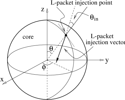
Figure 1: L-packet injection into the core: The packet is injected from a random point ($\theta$,$\phi$) on the surface of the sphere at such an angle ($\theta_{\rm in}$,$\phi_{\rm in}$) as to imitate an isotropic radiation field. The frequency of the injected packet is chosen from the Black (1994) radiation field.

The code used here is adapted for the study of cores having azimuthal symmetry. The core itself is divided into a number of cells by spherical and conical surfaces. The spherical surfaces are evenly spaced in radius, and there are typically 50-100 of them. The conical surfaces are evenly spaced in polar angle, and there are typically 10-20 of them. Hence the core is divided into 500-2000 cells. The specific number of cells used is chosen so that the density and temperature differences between adjacent cells are small.

The $L$-packets are injected from the outside of the core with injection point and injection direction chosen to mimic an isotropic radiation field incident on the core (see Fig. 1). We first generate the $L$-packet injection point on the surface of the core using random numbers $\mathcal{R}_{1},\mathcal{R}_{2}\leavevmode\nobreak\ \in\leavevmode\nobreak\ [0,1]$,

$$r = R_{\rm core}\,,$$ (4)

$$\theta = \cos^{-1}(1-2\mathcal{R}_{1})\;,$$ (5)

$$\phi = 2\pi\mathcal{R}_{2}\;;$$ (6)

and then the injection direction (Fig. 1), using random numbers $\mathcal{R}_{3},\mathcal{R}_{4}\leavevmode\nobreak\ \in\leavevmode\nobreak\ [0,1]$,

$$\theta_{\rm in} = \cos^{-1}\left(\mathcal{R}_{3}^{1/2}\right)\;,$$ (7)

$$\phi_{\rm in} = 2\pi\mathcal{R}_{4}\;.$$ (8)

Here $\theta_{\rm in}$ is the angle between the normal vector to the tangent plane at the point of entry and the packet injection vector, and $\phi_{\rm in}$ is the polar angle defined on the tangent plane.

We further assume that the radiation field incident on the core is the Black (1994) interstellar radiation field (hereafter BISRF), which consists of radiation from giant stars and dwarfs, thermal emission from dust grains, mid-infrared emission from transiently heated small grains, and the cosmic background radiation. This is a good approximation to the radiation field in the solar neighbourhood but it is not always a good choice when studying prestellar cores, since in many cases the immediate core environment plays an important role in determining the radiation field incident on the core. In this work, we simulate the effect of the immediate core environment by embedding the core in a molecular cloud which modulates the radiation field incident on the core. Another option is to estimate the effective radiation field incident on an embedded core by observing it directly (André et al. 2003).

The dust composition (and therefore the dust opacity) in prestellar cores is uncertain, but in such cold and dense conditions, dust particles are expected to coagulate and accrete ice. As in our previous study of prestellar cores (see Stamatellos & Whitworth 2003a), we use the Ossenkopf & Henning (1994) opacities for a standard MRN interstellar grain mixture (53% silicate and 47% graphite) that has coagulated and accreted thin ice mantles over a period of $10^{5}$ yr at a density of $10^{6}\;{\rm cm}^{-3}$.

3 Disk-like asymmetry

3.1 The model

The density profile in model cores with disk-like asymmetry is given by

$$n(r,\theta)=10^{6}\,{\rm cm}^{-3}\;\,\frac{1+A\left(\frac{r}{2000\,{\rm AU}}\right)^{2}{\rm sin}^{p}(\theta)}{\left[1+\left(\frac{r}{2000\,{\rm AU}}\right)^{2}\right]^{2}}\,.$$ (9)

Thus the density is approximately uniform in the centre, and falls off as $r^{-2}$ in the outer envelope. The core has a spherical boundary at radius $R_{\rm core}=2\times 10^{4}\,{\rm AU}$. The degree of asymmetry is determined by $A$ and $p$, and the values we have treated are given in Table 1, along with

$$e=\frac{\tau_{\rm V}(\theta=90\degr)}{\tau_{\rm V}(\theta=0\degr)}\,,$$ (10)

$M_{\rm core}$ and $\tau_{\rm V}(\theta=0^{\rm o})$. $e$ is the equatorial-to-polar optical depth ratio, i.e. the ratio of the maximum optical depth from the centre to the surface of the core (which occurs at $\theta=90\degr$) to the minimum optical depth from the centre to the surface of the core (which occurs at $\theta=0\degr$). Figure 2 displays isodensity contours on the $x=0$ plane for all the cases in Table 1.

Table 1: Model parameters for cores with disk-like asymmetry

Model ID	$A$	$p$	$e$	$M_{\rm core}/M_{\odot}$	$\tau_{\rm V}(\theta=0\degr)$
1.1	28	4	1.5	2.0	94
1.2	81	4	2.5	5.1	94
1.3	28	1	1.5	5.0	94
1.4	81	1	2.5	7.3	94

• Equatorial-to-polar optical depth ratio

• Core mass

• Visual optical depth from the centre to the surface of the core along the pole ($\theta=0\degr$).

3.2 Results: core temperatures, SEDs and images

In non-embedded cores, the dust temperature drops from around 17 K at the edge of the core to 7 K at the centre of the core, as previous studies have already indicated (Zucconi et al. 2001; Evans et al. 2001; Stamatellos & Whitworth 2003a). We also find that the dust temperature inside cores with disk-like asymmetry is $\theta$ dependent (see Figs. 3), similar to the results of Zucconi et al. (2001). As expected, the equator of the core is colder than the poles. The difference in temperature between two points having the same distance $r$ from the centre of the core but with different polar angles $\theta$, is larger for the more asymmetric cores (i.e. those with larger $e$ and/or $p$; Figs. 3). For example, at half the radius of the core ($10^{4}$ AU) the temperature difference between the point at $\theta=0\degr$ (core pole) and the point at $\theta=90\degr$ (core equator), is $5-6$ K for the $p=4$ models (Figs. 3a, 3b) but only $\sim 2$ K for the $p=1$ models (Figs. 3c, 3d). This temperature difference will affect the appearance of the core at wavelengths shorter than or near the core peak emission, where the Planck function is strongly (exponentially) dependent on the temperature.

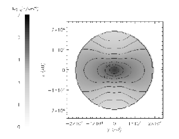
a

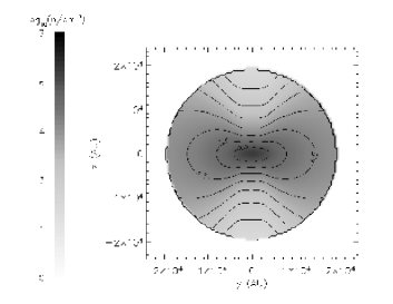
b

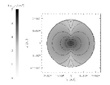
c

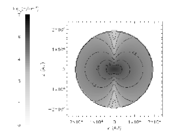
d

Figure 2: Density distribution on the $x=0$ plane (a) for a flattened asymmetric core with equatorial-to-polar optical depth ratio $e=1.5$ and $p=4$ (model 1.1), (b) for a more flattened asymmetric core, with $e=2.5$ and $p=4$ (model 1.2), (c) for a core with $e=1.5$ and $p=1$ (model 1.3), and (d) for a more flattened core, with $e=2.5$ and $p=1$ (model 1.4). We plot iso-density contours every $10^{0.5}{\rm cm^{-3}}$. The central contour corresponds to $n=10^{5.5}{\rm cm^{-3}}$.

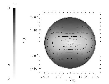
a

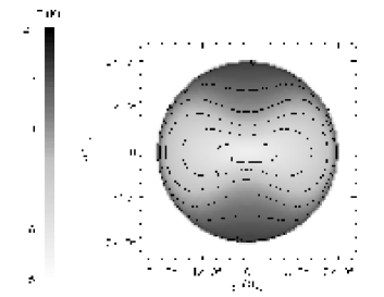
b

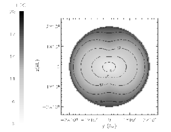
c

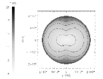
d

Figure 3: Temperature distribution on the $x=0$ plane, for the models presented in Fig. 2. We plot iso-temperature contours from 8 to 18 K, every 2 K.

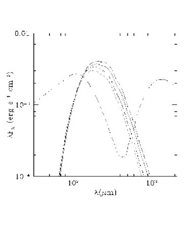
Figure 4: SED for the core models in Figs. 2, 3; model 1.1 ($e=1.5$, $p=4$; short-dashed line), model 1.2 ($e=2.5$, $p=4$; solid line), model 1.3 ($e=1.5$, $p=1$; dash-dot line) and model 1.4 ($e=2.5$, $p=1$;long-dashed line). The SED of each core is independent of the observer’s viewing angle. The dotted line on the graph corresponds to the incident/background SED.

The SED (Fig. 4) of a specific core, for the model parameters we examine, is the same at any viewing angle, because the core is optically thin to the radiation it emits (FIR and longer wavelengths). Thus, it is not possible to distinguish between flattened and spherical cores, using SED observations, unless the core is extremely flattened, so that it is optically thick on the equator at FIR and longer wavelengths. Using the Ossenkopf & Henning (1994) opacities, the minimum optical depth through the model core at $200\,\mu m$ is $2\tau_{\rm V}(\theta=0\degr)\times(\kappa_{200\mu m}/\kappa_{\rm V})\simeq 0.04$, so we would need to treat much larger values of $e$ ($\ga 25$) in order for the SED to be significantly dependent on viewing angle.

In contrast, the isophotal maps of a core do depend on the observer’s viewing angle. Additionally, they depend on the wavelength of observation. Our code calculates images at any wavelength, and therefore provides a useful tool for direct comparison with observations, e.g. at mid-infrared (ISO/ISOCAM), far-infrared (ISO/ISOPHOT) and submm/mm (SCUBA, IRAM) wavelengths. We distinguish two wavelength regions on which we focus: (i) wavelengths near the peak of the core emission (150-250$\leavevmode\nobreak\ \mu{\rm m}$; we choose 200$\leavevmode\nobreak\ \mu{\rm m}$ as a representative wavelength), and (ii) wavelengths much longer than the peak (submm amd mm region; we choose 850 $\mu{\rm m}$ as a representative wavelength). In each of the above regions the isophotal maps have similar general characteristics.

At 200 $\mu{\rm m}$ the core appearance depends both on its temperature and its column density in the observer’s direction. It is seen in Figs. 6-9, that cores with disk-like asymmetry appear spherical when viewed pole-on and flattened when viewed edge-on. The outer parts of a core can be more or less luminous than the central parts, depending on the core temperature and the observer’s viewing angle. For example, at close to pole-on viewing angles the outer parts of the core are more luminous than the inner parts of the core (limb brightening; e.g. Figs. 6-9, $\theta=$0°). This happens because the temperature is higher in the outer parts and this more than compensates for the lower column density (since at wavelengths near the peak of the core emission and shorter, the Planck intensity $B_{\nu}(T)$ depends on temperature as $B_{\nu}(T)\propto e^{-a/T}$, $a=$const). At other viewing angles the appearance of the core is determined by a combination of temperature and column density effects (Figs. 6-9, $\theta$=30°, 60°, 90°). This interplay between core temperature and column density along the line of sight results in characteristic features on the images of the cores. Such features include (i) the two intensity minima at almost symmetric positions relative to the centre of the core, on the images at 30°(Fig. 7-9), and (ii) the two intensity maxima, again at symmetric positions relative to the centre of the core, on the images at 90°(Figs. 6-7). (It is also worth mentioning that although the characteristic features appear in symmetric positions relative to both axes of density-symmetry, we should expect deviations from symmetry to arise if the radiation field incident on the core is not isotropic.)

We conclude that isophotal maps at 200 $\mu{\rm m}$ contain detailed information, and sensitive, high resolution observations at 200 $\mu{\rm m}$, could be helpful in constraining the core density and temperature structure and the orientation of the core with respect to the observer. In Fig. 5, we present a perpendicular cut through the centre of the core images shown in Fig. 7. We also plot the beam size of the ISOPHOT C-200 camera (90″, or 9000 AU for a core at 100 pc) and the beam size of the upcoming (2007) Herschel (13″or 1300 AU for the $170\leavevmode\nobreak\ \mu{\rm m}$ band of PACS; 17″or 1700 AU for the $250\leavevmode\nobreak\ \mu{\rm m}$ band of SPIRE). ISOPHOT’s resolution is probably not good enough to detect the features mentioned above. Indeed, a search in the Kirk et al. (2004) sample of ISO/ISOPHOT observations (also see Ward-Thompson et. al 2002) does not reveal any cores with such distinctive features. However, Herschel should, in principle, be able to detect such features in the future.

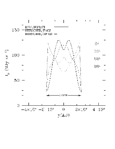
Figure 5: A perpendicular cut through the centre of the core images presented in Fig. 7 for model 1.2 at 200 $\mu{\rm m}$ (but also including the background radiation field). In addition we plot the beam size of ISO/ISOPHOT (90″$\equiv$ 9000 AU for a core at 100 pc) and the beam size of the upcoming (2007) Herschel (13″$\equiv$ 1300 AU for the $170\leavevmode\nobreak\ \mu{\rm m}$ band of PACS and 17″$\equiv$ 1700 AU for the $250\leavevmode\nobreak\ \mu{\rm m}$ band of SPIRE). ISO’s resolution may not be good enough to detect any of the features on the graph, but Herschel will have a much better resolution and should be able to detect such features in the future.

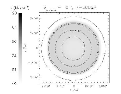
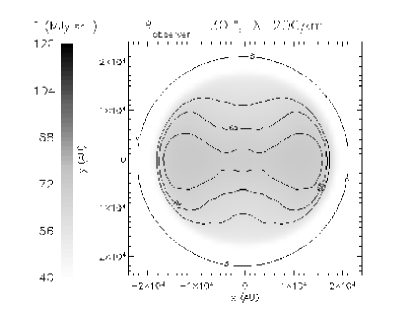
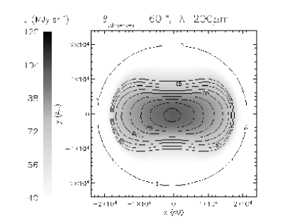
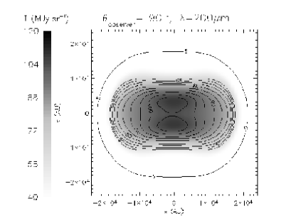
Figure 6: Isophotal maps at 200 $\mu{\rm m}$ at viewing angles $0\degr$, $30\degr$, $60\degr$ and $90\degr$, for a flattened core with equatorial-to-polar optical depth ratio $e=1.5$ and $p=4$ (model 1.1). We plot an isophotal contour at 5 MJy sr^-1 and then from 60 to 110 MJy sr^-1, every 5 MJy sr^-1. There are characteristic symmetric features due to core temperature and orientation with respect to the observer. We note that in these isophotal maps, and in all subsequent isophotal maps, the axes $(x,y)$ refer to the plane of sky as seen by the observer.

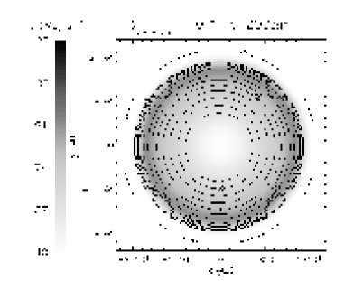
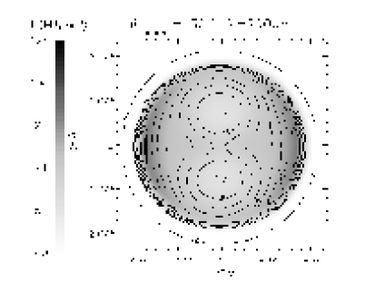
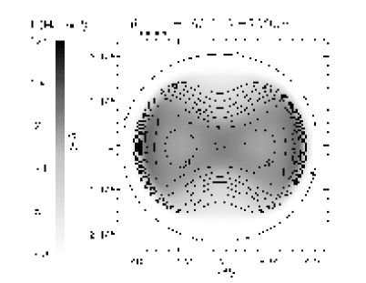
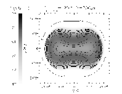
Figure 7: Same as Fig. 6, but for a more flattened core, with equatorial-to-polar optical depth ratio $e=2.5$ and $p=4$ (model 1.2).

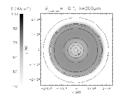
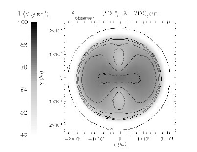
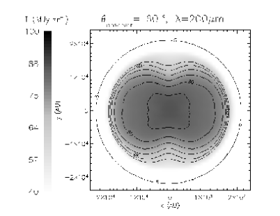
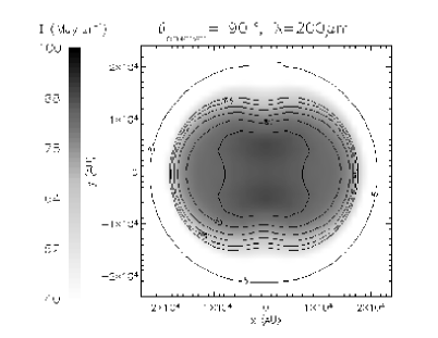
Figure 8: Same as Fig. 6, but for a core with equatorial-to-polar optical depth ratio $e=1.5$ and $p=1$ (model 1.3).

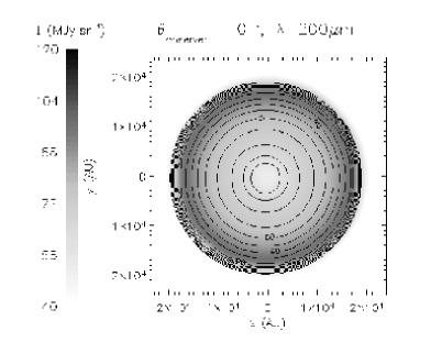
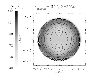
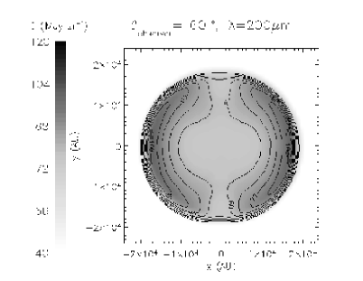
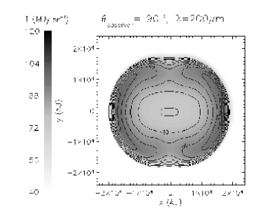
Figure 9: Same as Fig. 6, but for a core with equatorial-to-polar optical depth ratio $e=2.5$ and $p=1$ (model 1.4).

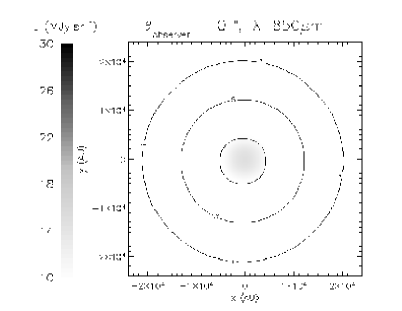
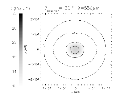
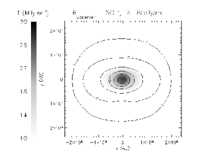
Figure 10: Isophotal maps at 850 $\mu{\rm m}$ at viewing angles $0\degr$, $30\degr$, $60\degr$ and $90\degr$, for a flattened core with equatorial-to-polar optical depth ratio $e=1.5$ and $p=4$ (model 1.1). We plot an isophotal contour at 1 MJy sr^-1 and then from 5 to 50 MJy sr^-1, every 5 MJy sr^-1. The core appears elongated when viewed at an angle other than $\theta=0\degr$.

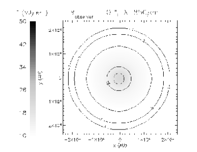
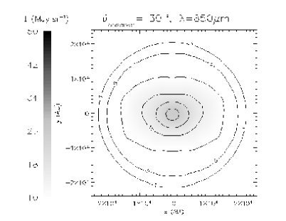
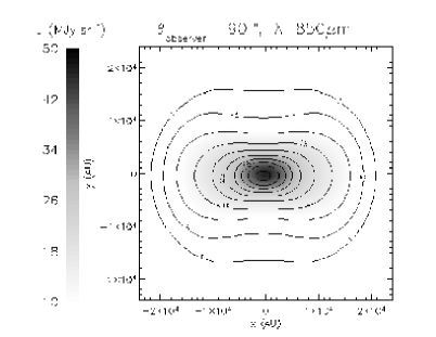
Figure 11: Same as Fig. 10, but for a more flattened core, with equatorial-to-polar optical depth ratio $e=2.5$ and $p=4$ (model 1.2).

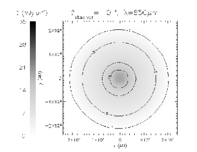
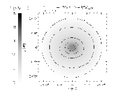
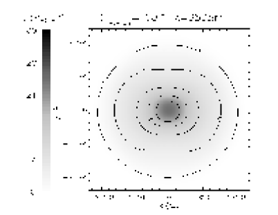
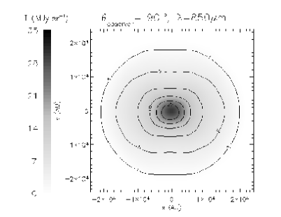
Figure 12: Same as Fig. 10, but for a core with equatorial-to-polar optical depth ratio $e=1.5$ and $p=1$ (model 1.3).

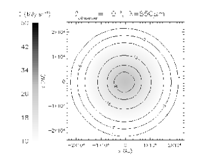
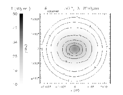
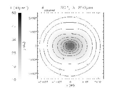
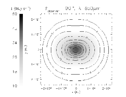
Figure 13: Same as Fig. 10, but for a core with equatorial-to-polar optical depth ratio $e=2.5$ and $p=1$ (model 1.4).

In the second wavelength region (submm and mm wavelengths) the core emission is mainly regulated by the column density (e.g. at 850 $\mu{\rm m}$, Figs. 10-13). Thus, the intensity is larger at the centre, where the column density is larger. For the same reason the core appears flattened when the observer looks at it from any direction other than pole-on. It is also evident that the peak intensity of the core is much larger when the core is viewed edge-on. Therefore, flattened cores are more prominent when viewed edge-on. This introduces a possible observational selection effect which should be taken into account when studying the shape statistics of prestellar cores. Low-mass flattened cores are more likely to be detected if they are edge-on, than if they are face-on. This is true for optically thin mm and submm continuum observations, and also for optically thin molecular line observations. For example, when comparing the projected shapes of condensations from hydrodynamic simulations with the observed shapes using solely optically thin continuum or optically thin molecular line observations, one should expect a lower number of observed near-spherical cores than indicated by the simulations. This may be the reason for the small excess of high axis ratio cores in the simulations by Gammie et al. (2003) (see their Fig. 9).

3.3 Embedded prestellar cores

In the previous section, we studied cores that are directly exposed to the interstellar radiation field (as approximated by the BISRF). However, cores are generally embedded in molecular clouds, with visual optical depths ranging from 2-10 (e.g. in Taurus) up to 40 (e.g. in $\rho$ Ophiuchi). The ambient cloud absorbs the energetic UV and optical photons and re-emits them in the FIR and submm (because the ambient cloud is generally cold, $T_{\rm cloud}\sim 20-100$ K). Therefore, the radiation incident on a core that is embedded in a cloud is reduced in the UV and optical, and enhanced in the FIR and submm (Mathis et al. 1983). Previous radiative transfer calculations of spherical cores embedded at the centre of an ambient cloud (Stamatellos & Whitworth 2003a), have shown that embedded cores are colder ($T<12$ K) and that the temperature gradients inside these cores are smaller than in non-embedded cores. André et al. (2003) also found that the temperatures inside embedded cores are lower than in non-embedded cores (assuming that they are heated by the same ISRF), using a different approach, in which they estimated the effective radiation field incident on an embedded core from observations.

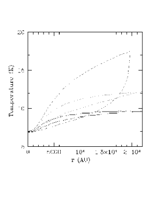
Figure 14: The effect of the parent cloud on cores. Temperature profiles of a non-embedded core (model 1.2; dashed lines), and of a core at the centre of an ambient cloud with visual extinction $A_{\rm V}=4$ (dotted lines), and $A_{\rm V}=13$ (solid lines). The upper curve of each set of lines corresponds to the direction towards the pole of the core ($\theta=0\degr$), and the bottom curve to the direction towards the core equator ($\theta=90\degr$). The core is colder when it resides inside a thicker parent cloud (i.e. when it is illuminated by a radiation field that is weakened at short ($<10\mu{\rm m}$) wavelengths), and the temperature differences between different parts of the core are smaller. Thus, the characteristic features on the isophotal maps at wavelengths near the peak of the core SED are weakened.

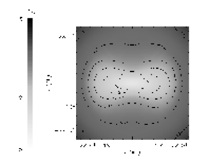
Figure 15: Temperature distribution on the $x=0$ plane, for the same model presented in Figs. 2b and 3b ($e=2.5$, $p=4$, model 1.2), but embedded in the centre of an ambient molecular cloud with visual extinction $A_{\rm V}=4$. We plot iso-temperature contours from 8 to 13 K, every 1 K. The embedded core is colder than the non-embedded core (Fig. 3b) and the temperature gradient inside the core is smaller.

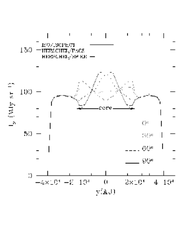
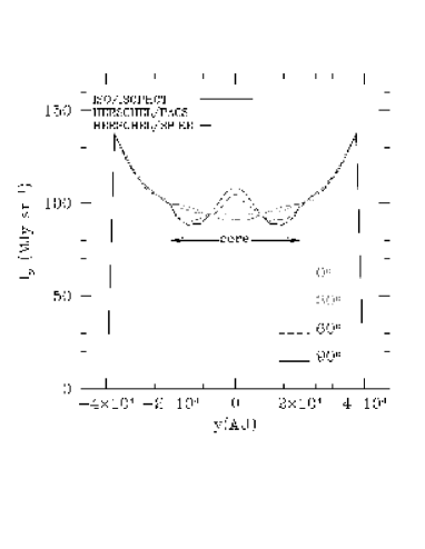
Figure 16: Same as Fig. 5, i.e. model 1.2, but for a core embedded in a uniform molecular ambient cloud with visual extinction $A_{\rm V}=4$. The characteristic features visible at different viewing angles are weaker than in the case of a non-embedded core.

Figure 17: Same as Fig. 5, i.e. model 1.2, but for a core embedded in a uniform molecular ambient cloud with visual extinction $A_{\rm V}=13$. There are two characteristic intensity minima visible at viewing angles 60^o and 90^o, but at viewing angles 0^o and 30^o these features are essentially invisible.

Here, we examine the more general case of embedded flattened cores. We model a core with the same set of parameters as model 1.2 ($p=4$, $e=2.5$) but embedded in a uniform density ambient cloud with different visual extinctions $A_{\rm V}$ ($A_{\rm V}=1.086\ \tau_{\rm V}$). The ambient cloud is illuminated by the BISRF. In Fig. 14, we present the temperature profiles at $\theta=0\degr$ (core pole; upper curves) and $\theta=90\degr$ (core equator; lower curves), (i) for a non-embedded core (dashed lines; model 1.2), (ii) for the same core embedded at the centre of an ambient cloud with $A_{\rm V}=4$ (dotted lines), and (iii) for the same core embedded at the centre of an ambient cloud with $A_{\rm V}=13$ (full lines).

Relative to an non-embedded core, a core embedded in an ambient cloud with $A_{\rm V}=4$ is colder and has lower temperature gradient (cf. Figs 3b and 15). The isophotal maps are similar to those of the non-embedded core (cf. Figs. 7 and 11), but the characteristic features are less pronounced. This is because the temperature gradient inside the core is smaller when the core is embedded (see Fig. 14). For example, at half the radius of the core ($r=10^{4}$ AU) the temperature difference between the point at $\theta=0\degr$ and the point at $\theta=90\degr$, is $5-6$ K for the non-embedded core, but only $\sim 1.5$ K for the same core embedded in an $A_{\rm V}=4$ ambient cloud. In Fig. 17 we present a perpendicular cut through the centre of the embedded core image at viewing angle 30°. It is evident that the features are quite weak, but they have the same size as in the non-embedded core (Fig. 5), and they may be detectable with Herschel, given an estimated rms sensitivity better than $\sim 1-3$ MJy sr^-1 at 170-250 $\mu{\rm m}$ for clouds outside the Galactic plane (dependent on cirrus confusion).

For a core embedded in an ambient cloud with $A_{\rm V}=13$, the temperature differences between different parts of the core are even smaller ($\la 1$ K at $r=10^{4}$ AU, see Fig. 14), but characteristic features persist (e.g. two symmetric intensity minima at 60°and 90°, see Fig.17).

Thus, continuum observations near the peak of the core emission, can be used to obtain information about the core density and temperature structure and orientation, even if the core is very embedded ($A_{\rm V}\sim 10-20$).

3.4 The effect of a UV-enhanced ISRF on embedded cores

We now examine the effect that a UV-enhanced ISRF has on the temperature profiles and isophotal maps of deeply embedded cores. We consider an ISRF that consists of the BISRF, plus an additional component of diluted blackbody radiation from stars with $T_{\star}=6000$ K or $T_{\star}=10000$ K, that illuminates isotropically the ambient molecular cloud in which the core resides. We use a dilution parameter $\omega_{\star}=10^{-13}$, so that the total additional luminosity illuminating the ambient cloud is

$$L=\omega_{\star}\,4\pi R_{\rm cloud}^{2}\,\sigma T_{\star}^{4},$$ (11)

where $\sigma$ is the Stefan-Boltzmann constant. This additional flux enhances the radiation at $\lambda=0.4\leavevmode\nobreak\ \mu{\rm m}$ incident on the ambient cloud by a factor of $\sim 3$ for $T_{\star}=6000$ K, and $\sim 30$ for $T_{\star}=10000$ K, as compared with the standard BISRF.

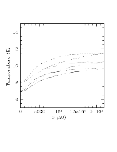
Figure 18: The effect of an UV-enhanced ISRF on embedded cores. Temperature profiles of a core with the same set of parameters as model 1.2 ($p=4$, $e=2.5$), embedded in a uniform density ambient cloud with visual extinction $A_{\rm V}=13$, that is illuminated by the BISRF (solid lines), by the BISRF plus a diluted blackbody of $T_{\star}=6000$ K (dotted lines) and by the BISRF plus a diluted blackbody of $T_{\star}=10000$ K (dashed lines). The upper curve of each set of lines corresponds to the direction towards the pole of the core ($\theta=0\degr$), and the bottom curve to the direction towards the core equator ($\theta=90\degr$). The core is hotter when the illuminating radiation field is enhanced at UV wavelengths, but the temperature differences between different parts of the core are not significantly increased.

In Fig. 18, we present the temperature profiles at $\theta=0\degr$ (core pole; upper curves) and $\theta=90\degr$ (core equator; lower curves) for a core with the same set of parameters as model 1.2 ($p=4$, $e=2.5$), embedded in a uniform density ambient cloud with visual extinction $A_{\rm V}=13$, illuminated by different ISRFs. The bottom pair of curves corresponds to illumination by the standard BISRF, and the upper two pairs of curves to illumination enhanced by a diluted blackbody with $T_{\star}=6000$ K and $T_{\star}=10000$ K. The core is hotter when the ambient cloud is illuminated by a more energetic UV field, by $1-2\leavevmode\nobreak\ K$ for the models we examine. The temperature differences between different parts of the core seem also to increase, but only by a small amount ($<0.5$ K). This means that the characteristic features on the isophotal maps at wavelengths near the peak of the core emission are not significantly changed.

For an even more energetic illuminating radiation field the enhancement would be larger. For example, the external UV radiation field incident on $\rho$ Ophiuchi is estimated to be $\sim 10-100$ times stronger than the BISRF, due to the presence of a nearby B2V star (Liseau et al. 1999). In this circumstance, we would expect cores to be hotter and the temperature differences may then be sufficiently large ($\sim 2$ K) to produce detectable features on isophotal maps at 200 $\mu{\rm m}$. However, if the illuminating radiation field is very much stonger than the BISRF, it is likely to involve significant contributions from a few discrete luminous stars in the immediate vicinity. It will therefore be markedly anisotropic and this will produce additional asymmetries in the isophotal maps, making their analysis more difficult.

Thus, continuum observations near the peak of the core emission may reveal features characteristic of the core structure even if the core is more deeply embedded ($A_{\rm V}>20$), provided that the radiation field incident on the core is sufficiently intense, and provided the effect of discrete local sources can be treated.

4 Axial asymmetry

4.1 The model

The density profile in model cores with axial asymmetry is given by

$$n(r,\theta)=10^{6}\,{\rm cm}^{-3}\;\,\frac{1+A\left(\frac{r}{2000\,{\rm AU}}\right)^{2}{\rm sin}^{p}(\theta/2)}{\left[1+\left(\frac{r}{2000\,{\rm AU}}\right)^{2}\right]^{2}}\,.$$ (12)

Thus – as with model cores having disk-like asymmetry – the density is approximately uniform in the centre, and falls off as $r^{-2}$ in the outer envelope; the core has a spherical boundary at radius $R_{\rm core}=2\times 10^{4}\,{\rm AU}$; and the degree of asymmetry is determined by $A$ and $p$. The values of $A$ and $p$ we have treated are given in Table 2, along with

$$e=\frac{\tau_{\rm V}(\theta=180\degr)}{\tau_{\rm V}(\theta=0\degr)}\,,$$ (13)

$M_{\rm core}$ and $\tau_{\rm V}(\theta=0\degr)$. $e$ is now the south-to-north pole optical depth ratio, i.e. the ratio of the maximum optical depth from the centre to the surface of the core (which occurs at $\theta=180\degr$) to the minimum optical depth from the centre to the surface of the core (which occurs at $\theta=0\degr$). Isodensity contours on the $x=0$ plane are plotted on Figure 2 for the model with $e=2.5$ and $p=4$.

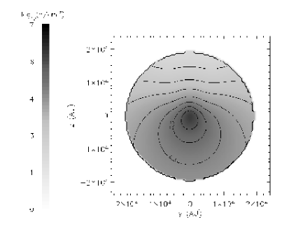
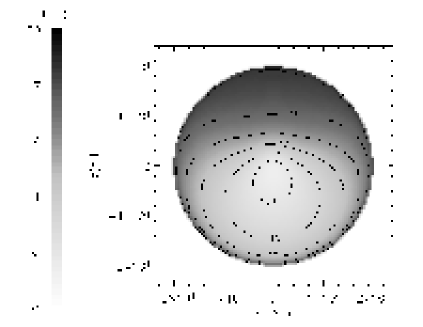
Figure 19: Density distribution on the $x=0$ plane for a core with axial asymmetry, south-to-north pole optical depth ratio $e=2.5$ and $p=4$ (model 2.2). We plot iso-density contours every $10^{0.5}{\rm cm^{-3}}$. The central contour corresponds to $n=10^{5.5}{\rm cm^{-3}}$.

Figure 20: Temperature distribution on the $x=0$ plane, for the model presented in Fig. 20 ($e=2.5$, $p=4$, model 2.2). We plot iso-temperature contours from 8 to 18 K, every 2 K. The denser, southern parts of the core are colder.

Table 2: Model parameters for cores with axial asymmetry

Model ID	$A$	$p$	$e$	$M_{\rm core}/M_{\odot}$	$\tau_{\rm V}(\theta=0\degr)$
2.1	28	4	1.5	1.4	94
2.2	81	4	2.5	3.4	94
2.3	28	1	1.5	2.4	94
2.4	81	1	2.5	6.3	94

• South-to-north pole optical depth ratio

• Core mass

• Visual optical depth from the centre to the surface of the core along the pole ($\theta=0\degr$).

4.2 Results: core temperatures, SEDs and images

In Fig. 20, we present the core density profile on the $x=0$ plane for model 2.2 ($p=4$, $e=2.5$), and in Fig. 20 the corresponding temperature profile. The temperature drops from $\sim 18$ K at the edge of the core to $\sim 7$ K at the centre of the core, and the denser “southern” parts of the core are colder. The difference between regions of the core with the same $r$ but different $\theta$ is larger for the $p=4$ models than for the $p=1$ models, and also larger for the more asymmetric models ($e=2.5$) than for the less asymmetric models ($e=1.5$). For example, at half the radius of the core ($10^{4}$ AU) the temperature difference between the point at $\theta=0\degr$ (core north pole) and the point at $\theta=180\degr$ (core south pole) is $\sim 7$ K for the $p=4$, $e=2.5$ model, $\sim 5$ K for the $p=4$, $e=1.5$ model, $\sim 4$ K for the $p=1$, $e=2.5$ model and $\sim 3$ K for the $p=1$, $e=1.5$ model.

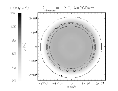
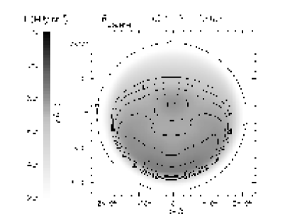
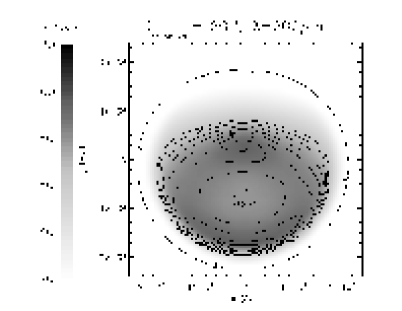
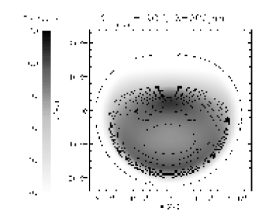
Figure 21: Isophotal maps at 200 $\mu{\rm m}$ at viewing angles $0\degr$, $30\degr$, $60\degr$ and $90\degr$, for a flattened core with south-to-north pole optical depth ratio $e=2.5$ and $p=4$ (model 2.2). We plot an isophotal contour at 5 MJy sr^-1 and then from 60 to 110 MJy sr^-1, every 5 MJy sr^-1.

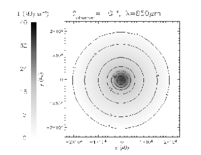
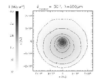
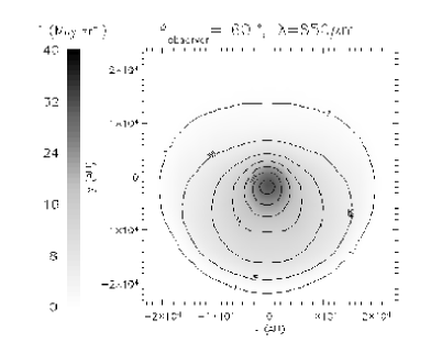
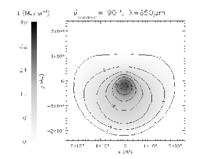
Figure 22: Isophotal maps at 850 $\mu{\rm m}$ at viewing angles $0\degr$, $30\degr$, $60\degr$ and $90\degr$, for a flattened core with south-to-north pole optical depth ratio $e=2.5$ and $p=4$ (model 2.2). We plot an isophotal contour at 1 MJy sr^-1 and then from 5 to 50 MJy sr^-1, every 5 MJy sr^-1. The core appears elongated when viewed at an angle other than $\theta=0\degr$.

As in the case of cores with disk-like asymmetry, these temperature differences result in characteristic features on isophotal maps at wavelengths near the peak of the core emission. In Fig. 21, we present 200 $\mu{\rm m}$ images at different viewing angles. The core appears spherically symmetric when viewed pole-on, but the effects of axial asymmetry start to show when we look at the core from other viewing angles (e.g. $30\degr$, $60\degr$ and $90\degr$). Comparing with the images at 200 $\mu{\rm m}$ for cores with disk-like asymmetry (Fig. 6-9), we see that for cores with axial asymmetry there is only one axis of symmetry. Thus, the symmetry of the characteristic features is indicative of the underlying core density structure. These features contain information about the core density, temperature and orientation with respect to the observer, and therefore observations near the peak of the core emission are important. The resolution of ISO/ISOPHOT was not high enough to detect such features.

The 850 $\mu{\rm m}$ images (Fig. 22) map the column density of the core along the line of sight. We point out the similarities between the maps in Fig. 22, and SCUBA observations of L1521F, L1544, L1582A, L1517B, L63 and B133 (Kirk et al. 2004). Further modelling for each specific core is required to make more detailed comparisons.

As in the case of cores with disk-like asymmetry, the SEDs of cores with axial asymmetry are independent of the observer’s viewing angle, because they are optically thin at long wavelengths.

5 Discussion

We have performed accurate two dimensional continuum radiative transfer calculations for non-spherical prestellar cores. We argue that such non-spherical models are needed because observed cores are clearly not spherically symmetric, and are not expected to be spherically symmetric. Our models illustrate the characteristic features on isophotal maps which can help to constrain the intrinsic density and temperature fields within observed non-spherical cores. They demonstrate the importance of observing cores at wavelengths around the peak of the SED and with high resolution.

Our main results are:

• For the cores treated here, which are optically thin at the long wavelengths where most of the emission occurs, the SED is essentially the same at any viewing angle. For example, in the case of cores having disk-like asymmetry, the SED does not distinguish between cores viewed from different angles.

• Isophotal maps at submm wavelengths (e.g. at 850 $\mu{\rm m}$) are essentially column density tracers, whereas maps at far infrared wavelengths around the peak of the core emission (e.g. 200 $\mu{\rm m}$) reflect both the column density and the temperature field along the line of sight. Therefore, sensitive, high-resolution observations at 170-250 $\mu{\rm m}$ (Herschel) combined with long-wavelength observations (e.g. 850 $\mu{\rm m}$ or $1.3\leavevmode\nobreak\ {\rm mm}$) can in principle be used to constrain the orientation of a core and the temperature field within it.

• If we assume a universal ISRF, then cores embedded in ambient molecular clouds are colder than cores directly exposed to the ISRF and have lower temperature gradients within them. As a result, the characteristic features on 200 $\mu{\rm m}$ isophotal maps are weaker for cores embedded in ambient clouds with visual extinction less than $A_{\rm V}\leavevmode\nobreak\ \sim\leavevmode\nobreak\ 10$, and may even disappear completely for more deeply embedded cores ($A_{\rm V}>20$).

• If the ISRF incident on the ambient molecular cloud is enhanced in the UV region (for example, by nearby luminous stars) but still isotropic, then the embedded cores are hotter and the temperature gradients inside them may be sufficient to produce detectable characteristic features, even in deeply embedded cores.

• The shapes of asymmetric cores depend strongly on the observer’s viewing angle. For example, cores with disk-like asymmetry appear more flattened when viewed edge-on. Our models also indicate that such cores should be easier to detect when viewed from near the equatorial plane. This may introduce a selection effect that should be taken into account when studying the statistics of the shapes of cores, using solely optically thin continuum, or optically thin molecular-line, observations.

• If the ambient ISRF is isotropic, the characteristic features on 200 $\mu{\rm m}$ maps are symmetric with respect to two axes for cores with disk-like asymmetry, and with respect to one axis for cores with axial asymmetry. Thus, just the symmetry of these features, could be indicative of the core’s internal density structure. Lack of symmetry in the features could indicate triaxiality, but it could also simply indicate that the radiation field incident on the core is anisotropic, due to discrete local sources.

Recently Gonçalves, Galli, & Walmsley (2004) have presented radiative transfer models of axisymmetric and non-axisymmetric toroidal cores, and also models of cores heated by an additional external stellar source. In their approach, they use a similar but independent Monte Carlo radiative transfer code. Their models focus on the effect of different core density profiles and anisotropic heating of cores, whereas we focus on the effect of observing mildly asymmetric cores at different viewing angles. Both studies are in general agreement for similar core models, and are helpful for the study of non-spherical realistic prestellar cores.

We are now extending our study by treating the effect of an anisotropic illuminating radiation field. We are also studying the triaxial molecular cores that result from 3-dimensional hydrodynamic simulations.