Patterns in the Outer Parts of Galactic Disks

Abstract

This paper describes test particle simulations of the response of the outer parts of Galactic disks to barring and spiral structure. Simulations are conducted for cold Mestel disks and warm quasi-exponential disks with completely flat rotation curves, subjected to pure quadrupoles and logarithmic spirals. Even though the starting velocity distributions are smooth, the end-points of the bar simulations show bimodality and multi-peaked structures at locations near the outer Lindblad resonance (OLR), although spirality can make this smoother. The growth of a bar may cause the disk isophotes to become boxy at the OLR, as stars accummulate particularly along the minor axis. The growth of a bar is also accompanied by substantial heating of the disk stars near the OLR. For the growth of a $10^{10}M_{\rm\odot}$ bar, the radial velocity dispersion is typically quadrupled for initially cold disks (initial $\sigma_{\rm u}$$\sim 10$  km s^-1), and typically doubled for disks with final $\sigma_{\rm u}$$\sim 45$  km s^-1. Simulations performed of the growth and dissolution of bars give very similar results, demonstrating that the heat once given to disk stars is very difficult to remove.

1 Introduction

The traditional approach to stellar dynamics, which stems from the work of Eddington and Jeans in the early years of the twentieth century, assumes that the phase space distribution of stars is smooth. From this innocent enough assumption, the remarkable and powerful Jeans (1915) theorem follows. This constrains the phase space distribution function to depend on the isolating integrals of motion only.

Nowadays, it is less clear that the assumption of a smooth distribution which underpins classical stellar dynamics is at all justified. For example, it has been realised that the local velocity distribution in the Galactic disk is deformed by stellar streams and moving groups (e.g. Eggen 1996a, Eggen 1996b). Members of such kinematically cold streams move with similar space motions. ? presented convincing evidence that the local distribution of stars is strongly bimodal. He identified two streams of stars, the Hyades and the Sirius superclusters. More recent pictures of the local stellar velocity distribution, obtained by ? with the Hipparcos data, revealed extensive clumps of structure in the $(U,V$) plane (i.e., the horizontal velocity plane) of disk stars.

The aim of this paper is to investigate the phase space structures that form in galactic disks using test particle simulations. Such structure may be generated by a number of dynamical mechanisms. As ? originally suggested, the growth of a bar may cause the trapping of stars in the vicinity of the outer Lindblad resonance and this is a possible explanation of the structures observed in the solar neighbourhood. Both the growth and the dissolution of bars are processes that are likely to have occurred in many disk galaxies (e.g. ?, ?) and it is interesting to look for possible diagnostics. Second, any spirality is also likely to buffet the stars and generate characteristic structures in phase space.

The paper is organised as follows. In Section 2, some details of the numerical procedure are given. The calculations are all test-particle simulations, as is applicable to the study of the outer parts of disk galaxies where the potential of the dark halo is important. Sections 3, 4, 5 and 6 study the effects of a bar and spirality, (alone as well as acting in concert with each other), on physical quantities such as the velocity distribution, dispersion, disk heating and surface density. Section 7 considers the growth and dissolution of bars and spiral arms.

2 Simulations

2.1 Equilibrium Models

I assume that the equilibrium disk is scale-free with a flat rotation curve. The form of the potential is:

$$\Psi=-v_{0}^{2}\ln\left(\frac{R}{R_{0}}\right).$$ (1)

Here, $v_{0}$ is the constant amplitude of the circular velocity curve, while $R_{0}$ is a characteristic lengthscale. The circling frequency $\Omega$ and the epicyclic frequency $\kappa$ are

$$\Omega={v_{0}\over R},\qquad\kappa={2v_{0}\over R}.$$ (2)

The outer Lindblad resonance (OLR) occurs at

$$R_{\rm OLR}=\left(1+{1\over\sqrt{2}}\right){v_{0}\over{\Omega_{\rm p}}}.$$ (3)

I always scale the pattern speed of the non-axisymmetric perturbation (${\Omega_{\rm p}}$) to unity, so that corotation (CR) occurs at a Galactocentric radius of $R_{0}$. Without loss of generality, both $R_{0}$ and $v_{0}$ are often set to unity.

The self-consistent distribution functions (hereafter DFs) depend on the isolating integrals of motion only. These are the binding energy per unit mass $E$ and the angular momentum component perpendicular to the plane of the disk $L_{z}$. The self-consistent DFs are (e.g. Chapter 4 in ?, ?)

$$f_{\rm s}(E,L_{z})=\tilde{C}L_{z}^{\gamma}\exp\left(-(\gamma+1){E/v_{0}^{2}}\right).$$ (4)

Here, $\tilde{C}$ is a normalisation constant, whose value can be found in ?. The velocity anisotropy constant $\gamma$ prescribes the radial and tangential second moments $\sigma_{\rm u}$² and $\sigma_{\rm v}$² of the stars. They are related to the anisotropy parameter $\gamma$ by:

$$\sigma_{\rm u}^{2}={\displaystyle{{v_{0}^{2}}\over{1+\gamma}}},\qquad\qquad\sigma_{\rm v}^{2}={\displaystyle{v_{0}^{2}}}.$$ (5)

The exponential surface density profile of a disk galaxy like ours is well-reproduced by the “doubly cut-out power law distribution functions” (?). The equilibrium distribution function of such a doubly cut-out disk is given as:

$$f_{\rm exp}(E,L_{z})=H(L_{z})f_{\rm s}(E,L_{z}).$$ (6)

Here, $f_{\rm s}$ represents the self-consistent DF given in (4), while $H(L_{z})$ is the cut-out function:

$$H(L_{z})=\frac{L_{z}^{N}L_{\rm c}^{M}}{[L_{z}^{N}+(v_{\beta}R_{0})^{N}][L_{z}^{M}+L_{c}^{M}]}.$$ (7)

Here, $N$ and $M$ are the inner and outer cut-out indices. They are chosen as positive integers and they control the sharpness of the inner and outer cut-outs respectively. The constant $L_{\rm c}$ is the angular momentum of a circular orbit at the cut-out radius $R_{\rm c}$. Here, $v_{\beta}$ is related to the rotation curve via:

$$v_{c}^{2}(R)=v_{\beta}^{2}\left(\frac{R_{0}}{R}\right)^{\beta}.$$ (8)

and $\beta$ is the index that controls the fall-off of the circular velocity with galactocentric radius.

Computation of the surface density corresponding to the doubly cut-out DF involves numerical integration. By choosing the relevant parameters carefully, the surface density profile of the disk can be made to look exponential. Such models are referred to as “quasi-exponential”.

In this paper, two models are used as standards. The first is a cold Mestel disk ($\gamma=600$, $\beta=0$), whose DF is given by eq. 4. This has a flat rotation curve. The second is a warm quasi-exponential disk ($\gamma=45$, $\beta=0$, $M=3$, $N=1$, $R_{\rm c}=2$), whose DF is given by eq. (6). Here, the rotation curve is still flat, as the halo provides the missing forces. The surface density of the models is shown in Figure 1.

Figure 1: The logarithm of the surface density is plotted as a function of radius. The quasi-exponential disk is characterised by a surface density profile that is well approximated by an exponential; it is represented by the dash-dotted straight-line. The $1/R$ surface density profile of the Mestel disk is shown by the solid line.

2.2 Perturbations

The general procedure is to set up initial positions and velocities corresponding to a smooth, equilibrium model. This equilibrium is subjected to perturbing forces $\Psi_{\rm p}(x_{\rm r},y_{\rm r})$ caused by a rotating bar or spiral pattern. The Cartesian coordinates in the rotating frame ($x_{\rm r},y_{\rm r}$) of the perturber, (with a pattern speed of $\Omega_{\rm p}$) are related to those in the inertial frame ($x,y$) by a rotational transformation about the angle ${\Omega_{\rm p}}t$. The perturbation potential is steady in time in the frame rotating with pattern speed ${\Omega_{\rm p}}$, so the components of the disturbing forces referred to the inertial frame ($f_{x},f_{y}$) are also related to the components in the rotating frame via a similar transformation.

This gives us the equations of motion as

$${\ddot{x}} =-{\displaystyle xv_{\beta}^{2}R_{0}^{\beta}\over\displaystyle R^{\beta+2}}+f_{x},$$

$${\ddot{y}} =-{\displaystyle yv_{\beta}^{2}R_{0}^{\beta}\over\displaystyle R^{\beta+2}}+f_{y}.$$ (9)

The orbits are then computed with either standard Runge-Kutta or leapfrog integrators.

After the perturbation reached full strength and the stellar system settled down, positions and velocities of the stars in the sample were recorded. I exploit the time averages theorem (?), which says that time averages are equivalent to phase averages for a steady-state system. Typically, $10^{3}$ orbits were evolved under the perturbing forces. These were each sampled randomly $10^{3}$ times after the potential had settled to its steady-state endpoint.

In order to compute the velocity moments and distributions, the spatial coordinates of the stars are placed on a grid that is regular in radius and azimuth. The kinematical data in each cell are used to construct the local bivariate velocity frequency distribution. Results are often shown as ($U$, $V$) contour plots, where $U$ is the radial velocity (measured positive towards the Galactic Center) with respect to the Sun, whilst $V$ is the azimuthal velocity (measured positive in the direction of Galactic rotation) with respect to the Sun. The solar peculiar motion is $U_{\odot}=5$ km s^-1and $V_{\odot}=10$  km s^-1(see e.g. ?).

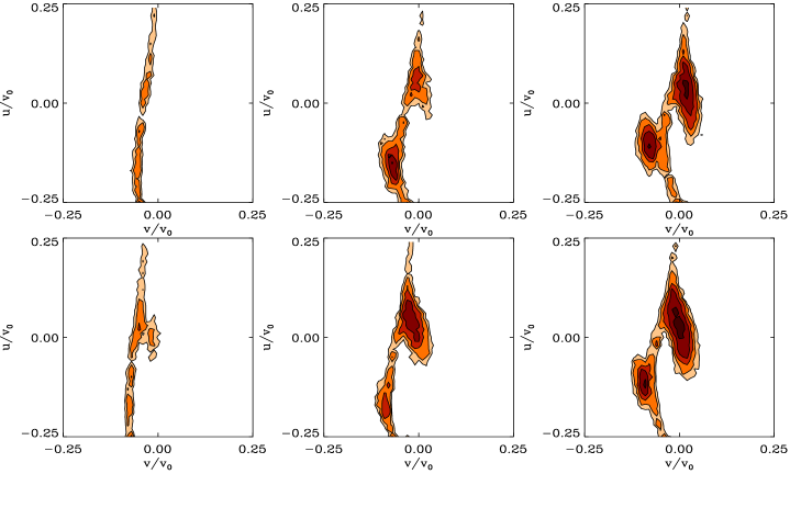
Figure 2: Plots of the velocity distributions in the ($U,V$) plane after the growth of a bar. The initial model is a cold Mestel disk. It is perturbed by a growing bar, the maximum strength of which is 1.8$\%$ of the gravitational field of the background disk, at the OLR. The upper three panels show the ($U,V$) distributions just within OLR at azimuths of roughly $25^{\circ},45^{\circ}$ and $65^{\circ}$. The lower three panels show the distributions just outside the OLR and at the same azimuths. The velocity distribution function decreases outwards as represented by the gradient in the shading.

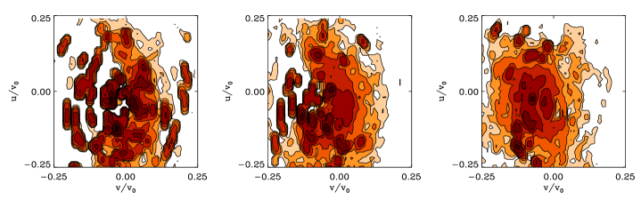
Figure 3: Plots of the velocity distributions in the ($U,V$) plane after a bar has perturbed an initially warm, quasi-exponential disk. The maximum bar field strength is 2.4$\%$ of the background field, at the OLR. The left panel shows the distribution at the OLR location while the other two panels are at radii further out. The observer is at an azimuth of 25^∘ in all these diagrams. The distribution diagrams have not been smoothed here. All other parameters are the same as Figure 2.

2.2.1 Bar

The first example presented below concerns the growth and dissolution of bars. As a simple model of the gravity field of a bar, I use a rigidly rotating quadrupole:

$$\Psi_{\rm bar}=\epsilon\frac{\cos(2\phi)}{R^{3}}$$ (10)

Here, $\phi$ is the azimuthal angle and $\epsilon$ is a measure of the strength of the bar. $\zeta$ is used to denote the ratio of the maximum of the radial force of the perturbation to that of the equilibrium potential at the OLR. The bar is grown adiabatically using the rule

$$\epsilon=\cases{\epsilon_{0}\tanh^{4}\Bigl{(}{\displaystyle t\over\displaystyle\tau}\Bigr{)}&if $t\geq 0$,\cr 0&otherwise.\cr}$$ (11)

Typically, orbits are computed in the axisymmetric potential for a time $2\tau$, then the bar is turned on and grows to its maximum strength over a growth time $4\tau$. After this, orbits are recorded over a period of $2\tau$. To ensure adiabaticity, $\tau$ is chosen such that the growth time is much larger than the revolution time of the bar.

2.2.2 Spiral Pattern

The second example of a perturbation is weak spirality, modelled as a logarithmic spiral. I use a spiral pattern with a pitch angle $i=15^{\circ}$ as motivated by observations of the Milky Way (?). Typically a 4-armed spiral pattern is used, with a pattern speed that is 21/55 times that of the bar, which is within the range thought to be valid for the Milky Way (?). This ratio places the ILR of the 4-armed spiral at the physical location of the OLR of the bar. On occasions, I also use 25/55 as the ratio of pattern speeds, which places the ILR of the spiral $\sim 20\%$ inward of the OLR of the bar.

The perturbation potential has the following form (eg. ?):

$$\Psi_{\rm spiral}=\epsilon K(\alpha,m)R_{0}e^{i(m\phi-\Omega_{p}t)}\left(\frac{R}{R_{0}}\right)^{i\alpha-\frac{1}{2}}.$$ (12)

Here $K(\alpha,m)$ is the Kalnajs Gravity function defined as:

$$K(\alpha,m)=\displaystyle{\frac{1}{2}\frac{\Gamma\left(\frac{1}{4}+\frac{m}{2}+\frac{i\alpha}{2}\right)\Gamma\left(\frac{1}{4}+\frac{m}{2}-\frac{i\alpha}{2}\right)}{\Gamma\left(\frac{3}{4}+\frac{m}{2}+\frac{i\alpha}{2}\right)\Gamma\left(\frac{3}{4}+\frac{m}{2}-\frac{i\alpha}{2}\right)}}$$ (13)

In Equation 12, $\epsilon$ is again a measure of the strength of the spirality. Again, this is related to the quantity $\zeta$, which we define to denote the ratio of the maximum of the radial force of the perturbation to that of the equilibrium potential at the ILR. For the same value of $\epsilon$, the maximum radial force due to the bar at its OLR is $\sim 25\%$ greater than that due to the spiral patten at its ILR. The spiral pattern is also grown adiabatically using the rule (11).

2.2.3 Bar and Spiral Pattern

As the third example of a non-axisymmetric perturbation, I have used both the quadrupolar bar and the standard logarithmic spiral pattern to perturb a background disk. At the OLR due to the bar, the value of $\zeta$ produced by the bar and spiral acting together, is about $1.6$ times that due to the bar alone and about $1.28$ times due to the spiral alone.

The orbital parameters are recorded in the rotating frame of the bar, in which the spiral pattern is not stationary. This adds an extra element of complexity to these simulations. In these smulations, if orbital data is recorded at random time points, (as is done in the bar-only or spiral-only simulations), then the effects of the perturbations are completely washed out, as the bar and spiral pattern are not synchronised. Thus, I record data only at those times when the bar and spiral pattern are at the same relative configurations. This is done by checking the phase of the potential of the bar against that of the spiral, on the corotation circle.

3 Velocity Distributions

Figs. 2 - 3 show the velocity distributions at the end of simulations for a cold Mestel disk and a warm quasi-exponential disk respectively. These disks have been perturbed by a bar; when added to the Mestel disk, the strength parameter for the perturbation is $\zeta=0.018$ and when imposed on the quasi-exponential disk, it is $0.024$. These numbers are chosen to bring out illustrative features in the results. In Figure 2, the top panels show a location just within the OLR, the bottom panels a location just outside the OLR. The velocity structure is shown at three angles to the bar’s major axis, namely $25^{\circ}$, $45^{\circ}$ and $65^{\circ}$. In Fig. 3, I only show plots at different radii.

Broadly speaking, it is observed that for the cold disk, the most distinctive feature of the corresponding velocity distribution is the presence of two clumps at most observer locations. As ? originally pointed out, and ? adumbrated, these clumps are built up from the families of stars on orbits that are aligned and anti-aligned with the long axis of the perturber. In the warm disk, the different stellar families are much less sharply defined on the $(U,V)$ plane. A larger portion of the velocity space is covered in the warm disk simulations.

Figure 4: At the same radius, (shown in dotted lines) the anti-aligned orbits (figure in solid lines, on the right) visible at low azimuths are sired by larger unperturbed orbits (shown by dashed lines) than those at high azimuths. Also, aligned orbits (figure in solid lines on the left) visible at low azimuths have relatively smaller progenitors. Azimuth is considered to increase with movement away from the bar major axis, in the first quadrant.

In terms of location in the $(U,V)$ plane, the clump representing stars on aligned orbits is centered around $U\approx 0$ and these stars generally have positive $V$ values. The clump representing the anti-aligned orbits generally lies in the quadrant $U<0$ and $V<0$. The distinction between these clumps becomes blurred as the background disk gets hotter. Roughly speaking, since the progenitors of anti-aligned orbits occur at relatively smaller radii, the stars on these initially unperturbed orbits experience stronger distorting forces than the progenitors of aligned orbits. (By “progenitor” of an orbit, I imply that circular orbit which when subjected to the perturbing potential, turns into the orbit at hand). This suggests that the eccentricity of the anti-aligned orbits will in general be higher than that of aligned orbits. The more eccentric an orbit, the greater is the radial excursion of the star. Thus, we can expect that the anti-aligned group in general will exhibit greater radial speeds than the aligned group. Initially circular orbits are distorted into anti-aligned orbits in the region between CR and OLR by the perturbing bar. Outside the OLR, circular orbits are deformed into aligned orbits. So, within the OLR, we expect many more anti-aligned orbits than aligned orbits. Outside the OLR, the converse is true. On this basis, we expect that the more populous clump inside the OLR represents the anti-aligned family of orbits, while the more populous clump outside the OLR represents the aligned family of orbits.

The velocity distributions change significantly with change in the azimuthal location of the observer, even at the same radius. Changes in populations of the aligned and anti-aligned families can be understood on the basis of orbital geometry. Figure 4 shows that the progenitors of anti-aligned orbits observed at a given radius and at low azimuths are larger than the progenitors of the anti-aligned orbits observed at the same radius but at higher azimuths. This size restriction on the progenitor at low azimuths implies that its radius typically exceeds $R_{\rm OLR}$ – in which case, the unperturbed orbit would be distorted into an aligned orbit rather than an anti-aligned one. As $R$ gets progressively smaller, the chance of the progenitor spilling outside the OLR reduces. Thus, at radii close to the resonance, there is a dearth of anti-aligned orbits observed at low azimuths. With increasing azimuth, the population in the anti-aligned family grows. As far as the aligned family is concerned, it is again true that in the vicinity of the resonance radius, at low azimuths there will be a scarcity of stars on aligned orbits. This is due to the fact that the progenitors of aligned orbits visible at low azimuths need to be smaller than those that distort into aligned orbits seen at high azimuth. The size requirement confines the initially circular orbit to $R<R_{\rm OLR}$, in which case it can only be distorted to an anti-aligned orbit. Again, the aligned family becomes more populated as the observer moves away from the resonance to higher radius. This is clearly shown in Fig. 2, in which the clumps at an azimuth of $65^{\circ}$ appear more populous than those at $25^{\circ}$.

Fig. 5 represents the heliocentric velocity distribution diagram obtained at the end of a simulation done with the standard spiral pattern imposed on an equilibrium quasi-exponential disk. The strength parameter $\zeta=0.0155$. The panels represent the distributions at the different radial locations of the observer. The left panel corresponds to the physical location of the OLR of an $m=2$ disturbance (such as a bar). This location is outside the ILR due to the spiral pattern used in the simulation, given a ratio of $25:55$ between the pattern speeds of the two perturbers. The middle and right panels are at progressively increasing radii outside the resonance location. The azimuthal location of the observer is $25^{\circ}$ for all the diagrams.

The velocity distribution diagrams obtained at the end of the simulation done with the standard bar and spiral simultaneously perturbing a quasi-exponential disk are represented in Figure 6. While the left panel represents the distributions at the location of the OLR due to the bar, the other panels are selected at progressively increasing radii. The panels exhibit the distributions at azimuths of $25^{\circ}$.

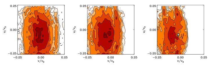
Figure 5: Plots of the velocity distributions in the ($U,V$) plane after the growth of the standard spiral pattern in a warm exponential disk. The chosen pattern speed of the spiral arm, places its ILR inside the physical location of the OLR of an $m=2$ perturbation of unit pattern speed. The left-most panel shows the distribution at this physical location. The other panels represent the picture at progressively increasing radii. All other parameters are the same as in Figure 3.

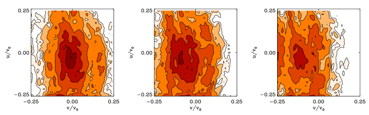
Figure 6: Plots of the velocity distributions in the ($U,V$) plane after the simultaneous growth of a bar and the standard spiral pattern. Details are the same as in Figure 5.

4 Velocity Dispersions

The bisymmetric nature of the perturbation at the OLR location, is clearly borne out in the Figures 7 $\&$  8. In fact, the $m=2$ symmetry comes out even more clearly when the bar perturbs a cold rather than a warm disk. This is because the stars are more restless in the warmer disk.

Figure 7: Plots of the variation of the velocity dispersion with position at the end of a simulation done with a bar imposed on the standard Mestel disk. The upper panels show the variation of $\sigma_{\rm u}$, $\sigma_{\rm v}$  and the cross-term $\sigma_{\rm uv}$,   with azimuthal angle, at the resonance location. Here, the field due to the bar is about $1.85\%$ that of the background disk. The lower panels show the variations with radius at three different azimuths, namely $25^{\circ}$ (solid line), $45^{\circ}$ (dashed line) and $65^{\circ}$ (dash-dotted line).

Figure 8: Plots of the variation of the velocity dispersion with position after the warm exponential disk has been perturbed by a bar. At the Outer Lindblad Resonance, the bar is about $2.4\%$ as strong as the background disk. All details are as in Figure 7.

The effect of the bar is most strongly imposed at the resonance location. Hence the radial velocity dispersion is expected to be highest at this radius. As far as the dependence of $\sigma_{\rm u}$  on azimuth is concerned, the perturbation due to the bar is strongest along its major axis and weakest along its minor axis, at any radius. Therefore we expect the radial velocity dispersion to be highest at $\phi=0$ and lowest at $\phi=\frac{\pi}{2}$, at the resonance. This is usually true as borne out by the panels showing the variation of $\sigma_{\rm u}$ with azimuth. It is reasonable to expect that the total velocity dispersion, at any radius, will be given by the depth of the potential at this location. Hence at any radius, the gradient in $\sigma_{\rm u}$,  (with change in azimuth) is expected to have the opposite sign to the change in $\sigma_{\rm v}$  as a function of azimuth. Thus tangential velocity dispersion is expected to be lowest along the major axis and highest along the minor at $R_{\rm OLR}$. However these trends are challenged when the intrinsic stellar velocity dispersion in the disk is high enough to impart sufficient energy to some of the stars to disobey the perturbing potential.

Figure 9: As in Figure 7 except that in this case, the standard spiral pattern perturbed a cold Mestel disk. The upper panels show the variation of velocity dispersions with azimuthal angle, at the location of the ILR due to the $4$ armed spiral pattern (which corresponds roughly to the OLR location due to the bar since the ratio of pattern speeds of the bar and the spiral pattern is 55:21 in this simulation). The gravitational field due to this spiral pattern is about $1.5\%$ that of the background disk at this radius.

The azimuthal dependence of the dispersions is shown at the ILR of to the spiral pattern in Figure 9. At this radius, the potential of the logarithmic spiral achieves maxima at a non-zero value of azimuth. Therefore, radial velocity dispersion peaks and tangential velocity dispersion dips at this azimuth rather than at $0^{\circ}$ as in Figure 7. Again, as in the bar simulations, these trends are not maintained in the warmer disk. As expected, the four-fold symmetry of the imposed spiral pattern manifests itself in the variation of the velocity dispersions with azimuth, at the ILR due to the spiral pattern (which is also the OLR location due to the bar, approximately). The symmetry comes out much more clearly in the simulation done with the colder Mestel disk than the warm quasi-exponential disk. The symmetry is most marked at the resonance location since the perturbation is felt most strongly here. As the spiral pattern is quite tightly wound, (i = $15^{\circ}$) the perturbation appears to be approximately axisymmetric. Consequently, the effect of the spiral arms at different azimuths and a given radius is almost the same.

5 Heating Results

The imposed perturbation heats the equilibrium disk depending on its strength. One measure of the heating is the ratio of the final location-averaged velocity dispersion to the average dispersion in the equilibrium disk. These “average” dispersions are easily calculated as follows. Once the orbits are recorded, the orbital data is gridded according to location and the local velocity dispersion calculated.

Let the velocity dispersion at the $i^{\rm th}$ location bin be $\sigma_{\rm i}$, the number of stars remaining in this location bin after the growth of the perturbation be $n_{\rm i}$ and the arithmetic mean of velocities of these $n_{\rm i}$ stars be $\mu_{\rm i}$. Let there be $N$ such location bins in total. The average variance of all the $\sum_{\rm i=1}^{N}{n_{\rm i}}$ stars is then given by:

$$\langle\sigma\rangle^{2}={\displaystyle{\frac{\sum_{\rm i=1}^{N}(\sigma_{\rm i}^{2}+\mu_{\rm i}^{2})n_{\rm i}}{\sum_{\rm i=1}^{N}{n_{\rm i}}}}}-{\left[{\displaystyle\frac{\sum_{\rm i=1}^{N}{\mu_{\rm i}n_{\rm i}}}{\sum_{\rm i=1}^{N}{n_{\rm i}}}}\right]^{2}}$$ (14)

The plots presented in Figure 10 show that the effect of imposing the bar on the standard cold Mestel disk is to elongate the radial velocity axis of the velocity ellipsoid more than the tangential velocity axis. Thus, the ellipsoid is distorted due to the perturbation. It is also observed in the figure, that heating increases in general, as the bar grows stronger.

Figure 10: Plot of the ratio of final to initial $\langle$$\sigma_{\rm u}$$\rangle$ (unbroken line) and $\langle$$\sigma_{\rm v}$$\rangle$ (broken line) in a cold Mestel disk, perturbed by a bar. The bar strength is the ratio, (expressed as a percentage) of the gravitational fields due to the bar and the background disk, at OLR. The unfilled circles represent the calculated values of the change in the velocity dispersions for different bar strengths, while the lines represent smooth fits to these data.

Figure 11 represents heating caused by the bar, the spiral pattern and the two together, when they perturb a warm exponential disk. Heating is plotted as a function of perturbation strength $\zeta$. The heating diagrams in Figure 11 show that velocity dispersions generally increase with increasing perturbation strength. Tangential heating is always less than radial heating at all perturbation strengths. It can be seen in Figure 11 that for a given ratio between the gravitational field due to the perturber and the disk, in general heating is maximum for a given perturbation strength, when the bar acts alone.

Figure 11: Plot of the ratio of final to initial $\langle$$\sigma_{\rm u}$$\rangle$ (unbroken line) and $\langle$$\sigma_{\rm v}$$\rangle$ (broken line) as a function of the ratio of the maximum field exerted by the perturbation to the field due to the disk ($\zeta$), obtained at the end of simulations in which a warm quasi-exponential disk is perturbed by a bar (left panel), the standard spiral pattern (middle panel) and a bar and the standard spiral (right panel). The ratio of the maximum radial force due to a quadrupole, a tightly wound logarithmic spiral and the quadrupole $\&$ spiral together, (all of unit strengths) to that of the background disk, at the OLR, is given by $1:1.25:1.6$.

The spiral pattern alone is the least efficient heating mechanism. In fact, around the ILR due to the spiral arms, the location-averaged disk heating is less than that around the OLR due to a bar of the same perturbation strength $\zeta$. A spiral pattern that is quasi-stationary cannot efficiently heat the stellar disk. This follows from the smooth, largely unchanged nature of the velocity distribution away from the resonances.

6 Surface Density Profile

I have investigated the response of the disk to the perturbation by plotting the number of stars at a given azimuthal location as a function of radius. This number is referred to as the “occupation number” in the paper. In fact, the integration of the surface density over a small local patch of the disk, provides the occupation number at that location. The occupation number in an equilibrium Mestel disk is a constant, independent of radius, while it has a more complicated dependence on radius for a disk with an initially exponential surface density profile.

6.1 Bar

The ratio of the final to the initial occupation numbers obtained at the end of simulations done with a bar, imposed on the standard Mestel and the quasi-exponential disks, is plotted as a function of the radial location of the observer, at different azimuths in Fig. 12.

Figure 12: Plot of the variation of the final to initial occupation numbers with radius when a bar is used to perturb the equilibrium disk; the panel on the right corresponds to the standard quasi-exponential disk and that on the left to the standard Mestel disk. The solid line represents the azimuthally averaged ratio of the final and initial occupation numbers while the dotted and the dash-dotted lines represent the ratio at azimuths of $90^{\circ}$ and $0^{\circ}$ respectively. In this case, $\zeta=1.8\%$.

It is observed that there is a depletion of stars from the region along the major axis of the bar ($0^{\circ}$) and an accumulation along the minor axis ($90^{\circ}$); this depletion and accumulation is strongest near the resonance radius. The variation in the occupation number is basically similar for both the exponential disk as well as the Mestel disk. As has been explained in Section. 3, there is a dearth of stars on both aligned and anti-aligned orbits at low azimuths, near the resonance. This shows up in the occupation number plot as a depletion at $\phi=0^{\circ}$, near the resonance location. Near the resonance, at high azimuths, both the orbital families are strong; however the aligned family gets thinner as radius decreases and the anti-aligned is progressively debilitated as radius increases. Thus there is a peak in the occupation number along the minor axis of the bar, near $R_{\rm OLR}$.

When the disk is much hotter, more stars can travel from outside the resonance to inside and vice versa. Thus the cause for the depletion and accumulation of stars along certain directions is less prominent in a warmer disk. Also, when the initial occupation number profile of the background disk is more exponential than flat, many more stars can come over from radii $<\;R_{\rm OLR}$, thus keeping the anti-aligned family well populated even at the low azimuths. These factors imply the flatter nature of the occupation number profiles when the bar is imposed on a warm exponential disk.

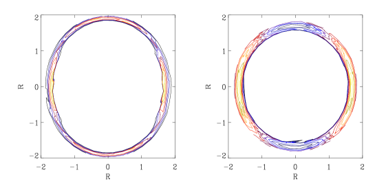
Figure 13: Isodensity contours in the vicinity of the OLR location when the bar perturbs the cold disk (left panel) and the warm disk (right panel). All other parameters are as in Figure 12. The bar is along the horizontal.

The ability of the bar to distribute stellar matter at the resonance location, across azimuths is also manifest in the isodensity contours turning boxy. Figure 13 depicts isodensity contours for which the occupation number calculations were shown in Figure 12. As is evident from the plots in this latter figure, the dip in the occupation number at low azimuths occurs just inside the OLR radius in the cold disk and just outside this location in the warmer disk. This explains why the contours shown in Figure 13 are anti-aligned to the bar in the colder disk (left panel of Figure 13) and aligned to the bar major axis in the warmer disk (right panel). In both cases, the contours are boxy though the deviation from an elliptical shape is more conspicuous in the cold disk case. The effect of the bar is less strong in the warm disk case as is evident from Figure 12, thus contributing to the boxiness of the isodensity contours to be less marked.

6.2 Spiral Pattern

Fig. 14 shows the variation in the ratio of the final occupation number to the same in the initially unperturbed equilibrium disk, at selected azimuths, with radius. As was explained in Section 4, the standard pattern is approximately axisymmetric. This implies that the effects of the spiral arms will be nearly isotropic on the disk. This explains why occupation number is almost the same at all azimuths. It appears from Fig. 14 that the spiral pattern tends to deplete stars away from lower radii and allow them to accumulate at higher radii. This can be attributed to more efficient angular momentum transfer from lower to higher radii, by the spiral as compared to the bar. In fact, the ILR due to the spiral, is an “emitter” of angular momentum, (?). Thus we expect to find a re-distribution of disk surface density towards higher radii, in the immediate neighbourhood of the ILR. The spiral pattern is not efficient in such re-distribution of matter at radii other than the resonances.

Figure 14: Plot of the variation of the final to initial occupation numbers with radius when the equilibrium disk is perturbed by a spiral pattern. The choice of the pattern speed of this spiral, implies that the ILR of this spiral pattern lies almost on top of the OLR due to an $m=2$ disturbance, such as a bar. In this case, $\zeta=1.125\%$. All other details are as in Fig. 12.

In the warm quasi-exponential disk, stars have higher random motion and the effect of the perturbation is manifest to a lesser degree. Thus occupation number varies more with azimuth in the right panel in Fig. 14 than in the left.

6.3 Bar and Weak Spiral Pattern

Figure 15: Plot of the variation of the final to initial occupation numbers with radius when the equilibrium disk is perturbed by the bar and the standard spiral pattern, jointly. In this case, $\zeta=3.8\%$. All other details are as in Fig. 14.

In Fig. 15 the ratio of the final occupation number to the initial occupation number in the unperturbed equilibrium disk, is plotted as a function of radius at chosen azimuths. Here the disk is perturbed by the bar and the spiral pattern jointly. We have seen in Fig. 12 that there tends to be a depletion of stars from the region along the major axis of the bar and an accumulation along the minor axis. The spiral pattern appears to drag stars away from lower radii, outwards. Both these effects are superimposed to produce the picture presented in Fig. 15.

7 Growth and Dissolution of a Bar and a Spiral Pattern

It is interesting to examine the extent to which the disk is able to retain memory of the phase space features caused by non-axisymmetric perturbations. This spurred the study of the effects of an imposed bar and the standard 4-armed spiral pattern, on disk stellar kinematics, as a function of the time periods over which the perturbation is grown ($T_{1}$) and dissolved ($T_{3}$) as well as the time over which the perturbation strength remained saturated to its maximum value ($T_{2}$). In these simulations, the “growth time” is equated to the “dissolution time” of the perturbation, ($T_{1}=T_{3}$). $T_{2}$ is referred to as the “steadiness time”. I first present the effects of a bar on a cold Mestel disk and follow this up with an investigation of the effects brought about by a bar and spiral pattern on a warm exponential disk.

7.1 Mestel Disk

Fig. 16 displays the location-averaged radial and tangential heating produced by a bar that is imposed on a cold Mestel disk and subsequently dissolved. It is observed that the bar-induced heating initially decreases rapidly with increasing growth time for a constant $T_{2}$, but very soon the rate of decrease becomes nearly zero. The degree of distortion of the velocity ellipsoid remained a constant approximately.

The trends manifest in Figure 16 can be understood in the light of the following discussion. When the bar is being grown and dissolved quickly, it is expected that stellar velocities in the disk will be rendered high. The slower the growth (and dissolution), the more nearly adiabatic and reversible are the conditions; so the smaller the final heating. Thus, there is higher disk heating at smaller values of $T_{1}$.

As the bar is grown (and killed) progressively slowly, there appears to be a range of the growth (and dissolution) time over which heating remains nearly a constant; (heating drops with even slower growths). This range in $T_{1}$ has been captured in Fig. 16. As the bar is dissolved more slowly, phase mixing becomes more efficient in the disk; thus it is not surprising that heating drops with increase in $T_{1}$ and $T_{3}$. Phase mixing is more efficient in the warm quasi-exponential disk than in the initially cold Mestel disk. Therefore we would expect a faster drop in disk heating with $T_{1}$ (=$T_{3}$) in the former than the latter configuration. This is borne by a comparison of Fig. 16 and Fig. 17.

I have noted in the experiments that the time over which the bar is allowed to remain at its maximum strength ($T_{2}$) does not affect heating, for fixed $T_{1}$ and $T_{3}$, as long as $T_{2}$ is sufficiently high. The disk heating recorded after the dissolution of the bar is determined by the efficiency of phase mixing. If $T_{2}$ is higher than a few bar rotation periods, the orbital eccentricities induced by the bar saturate and any further increase in $T_{2}$ will not distort the orbits. Roughly speaking, orbital eccentricities can be used as indicators of disk heating. Thus, enhancing the “steadiness time” beyond a point will not bring about any change.

As expected, heating depends sensitively on the bar strength for given values of $T_{1}$ (=$T_{3}$) and $T_{2}$.

Figure 16: Plot of variation in the disk heating caused by a bar which is grown and subsequently dissolved in the standard Mestel disk. The ratio of the final to the initial average radial velocity dispersion (solid line) and the same for the tangential velocity dispersion (broken line) is plotted as a function of the ratio of the “growth time” (or “dissolution time”) to the “steadiness time”, ($T_{1}/T_{2}$). The heating, as calculated at a value of the ratio $T_{1}/T_{2}$, is marked by unfilled circles, while the lines are smooth fits to these data. The bar strength is allowed to reach a maximum value that corresponded to $1.2\%$ of the background field at the OLR.

7.2 Warm Quasi-exponential Disk

Figure 17: Plot of variation in the disk heating caused by a bar (left panel) and the standard spiral pattern (right panel), which are grown and subsequently dissolved in the warm quasi-exponential disk. The ratio of the final to the initial average radial velocity dispersion (solid line) and the same for the tangential velocity dispersion (broken line) is plotted as a function of the ratio of the growth (or dissolution) time to the growth time, ($T_{1}/T_{2}$). The lines are actually smooth fits to the heating data, which is represented by unfilled circles. The bar contributes a maximum field that is $1.8\%$ of the background field, while the maximum field due to the spiral pattern is only $0.75\%$ of the field due to the Mestel potential, at the OLR due to the bar.

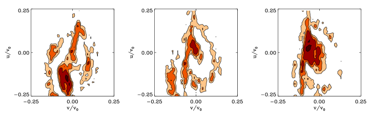
Figure 18: Plot of velocity distribution diagrams at the end of simulations in which a bar is grown and subsequently dissolved in the warm exponential disk. The panels represent observer radial locations which are inside, at and outside $R_{\rm OLR}$, at an azimuth of $25^{\circ}$. The velocity distribution is maximum at the centre and decreases outwards in these plots, as indicated by the gradient in the shading. The bar used in this simulation implies a maximum field that is $1.8\%$ of that of the background disk, at OLR. The growth (dissolution) time is 5 times the steadiness time, in this simulation.

Fig. 17 explores the disk heating that is caused when a bar (left panel) or a spiral pattern (right panel) is grown in a warm exponential disk and is then dissolved. The location-averaged radial and transverse heatings are plotted as functions of the ratio $T_{1}/T_{2}$. The degree of heating due to the spiral is much lower than that due to the bar in general.

Simulations were done in which a bar was grown and dissolved in a warm quasi-exponential disk. Heliocentric velocity distributions were recorded at the end of such simulations at different locations of the observer. In Fig. 18, a set of velocity diagrams representing the structures in velocity space after dissolution of the bar at the end of moderately long growth and dissolution times, are shown in the ($U-V$) plane at locations inside, at, and outside the OLR due to the bar at an azimuth of $25^{\circ}$. These structures obtained with an initially warm quasi-exponential disk are reminiscent of the features observed after a bar has been grown in a cold disk, (shown in Fig. 2), insofar as the two stellar families of oppositely oriented orbits are concerned. However, velocity distribution diagrams obtained at the end of simulations done with smaller values of the ratio ($T_{1}/T_{2}$), exhibit structure that is less well-defined.

The visual appearance of the structures in Fig. 18 suggests that they resemble the velocity distribution plots, obtained after stirring a cold disk with a bar, except that now, there are regions of phase space which are not occupied. Such “holes” are observed in the distributions irrespective of how slowly the bar is grown and dissolved. This observation is due to the fact that initially circular orbits that lay very close to the OLR, can become chaotic, by the introduction of the bar. In an action diagram, in the immediate vicinity of the resonance location, such orbits are known to occupy discontinuous patches, (?). The missing actions correspond to missing phase-space volumes. Thus, parts of the recorded velocity distributions are noted to be empty. These “holes” will be observed even when the perturbation potential is changed in the adiabatic limit.

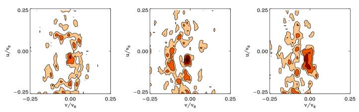
Figure 19: Plot of velocity distribution diagrams at the end of simulations in which the standard 4-armed spiral pattern is grown and subsequently dissolved in the warm exponential disk. The panels represent observer radial locations which are inside, at and outside the ILR due to the spiral pattern, at an azimuth of $25^{\circ}$. The maximum field contributed by the spiral pattern is about $1.5\%$ of that due to the background disk, at the ILR. In this simulation, $T_{1}/T_{2}=8$.

The velocity distribution diagrams in the vicinity of the ILR due to the standard spiral pattern (which corresponds very closely to the location of the OLR due to the bar), as recorded by an observer at the Sun, at the end of a simulation in which the spiral pattern is grown and then dissolved in a warm exponential disk, is shown in Fig. 19. Structures in the velocity space can be recognised from these figures. Again, as for the case of the bar, these distributions resemble velocity distribution plots, obtained by stirring a cold disk with a spiral pattern, except that the current plots exhibit missing patches of phase-space volume.

8 Conclusions

This paper presents test particle calculations showing the effects of bars and spiral patterns on the outer parts of galactic disks. The effects of the perturbations on the properties, such as the velocity dispersions and the stellar density, have been examined in detail. The changes are most pronounced at the resonance locations of the bars and spirals.

The simulations begin from idealised infinitesimally thin disks with smooth velocity distributions that are generated from the collisionless Boltzmann equation. Even so, the effects of the bar and spiral distortions cause the final velocity distributions to be far from smooth. Tightly-wound, many-armed spiral patterns do least damage to the smoothness of phase space, whereas bars cause much more disturbance.

The effects of the imposed perturbations are enumerated as follows.

1. In the model in which a cold disk is perturbed by a bar, Kalnajs’ mechanism causes definite bimodality at locations near the OLR. This effect is very clean in the cold disk, and the clumps can be readily identified with the families of aligned and anti-aligned orbits. However if a warmer disk is so perturbed, then the structure shows complex and multiple peaks, caused by the scattering of the original orbits onto resonant families. Spiral patterns do not cause bimodality.

2. The resonances can be locations of anomalous heating. This effect is most evident in results obtained from simulations done with completely cold disks, in which the imposition of a bar or a spiral pattern causes a peak in the radial component of the velocity dispersion $\sigma_{\rm u}$  at the resonance. When the disk is hotter, then the velocity dispersions are increased by any perturbation, but $\sigma_{\rm u}$  may either increase outward or decrease outward depending on the azimuth.

3. The resonances may also be locations where the disk isophotes are distorted from ellipses and are boxy. The effect of a bar is found to be to cause stars to become depleted from the major axis and accumulate on the minor axis at the OLR. Boxiness of isophotes has been associated with the presence of a bar by other workers, both in numerical (?) and observational studies (?), but only till about the bar length. The occupation number investigation reveals that the bar can act in a similar way, even in the outer disk, around the OLR. Spirality causes stars at the ILR (of the spiral) to gain angular momentum and drift outward. When a spiral pattern and a bar are made to act in conjunction, the degree of the inflicted boxiness on the isophotes is less than when the bar is acting alone.

4. Computations have been carried out to calculate the typical heating effects of bars and spiral patterns in the outer parts of galactic disks. For a typical galaxy like the Milky Way, we expect the growth of the bar to have roughly doubled or quadrupled the velocity dispersion, depending on whether the initial configuration was hot or cold. For disks presently like the Milky Way (with $\sigma_{\rm u}$$\sim 45$ km s^-1), the radial velocity dispersion is increased by a factor $f\approx 1+0.19\zeta_{\rm bar}$. Here, $\zeta_{\rm bar}$ is the ratio of the maximum gravitational field of the bar to that of the disk at the OLR. Spiral features are found to be much less efficient at heating the outer parts of galactic disks.

5. Runs in which bars are grown and dissolved indicate that the heating that accompanies the growth cannot be removed immediately on dissolution. A very rapid growth and dissolution of a bar the size of the Milky Way’s in an initially cold disk may cause the velocity dispersion to more than quadrupole in value. A less massive bar has a smaller effect, as does a hotter disk and longer growth (and dissolution) periods.

6. Another legacy left behind by the dissolved perturbers is on the velocity distributions. When the perturbers are grown and subsequently dissolved in a warm disk, the velocity distributions resemble those obtained after the perturbation reaches maximum strength in an initially cold disk, except that “gaps” appeared in the velocity space. These are caused by missing orbits that cannot retrace their steps once the perturbation is removed. This phenomenon has been earlier noted by Binney & Spergel (1984).

The simulations reported in this work attempt to understand the effect that imposed perturbations have on galactic disks, in general. A future paper is planned in which the models studied herein are explored in depth with the aim of replicating the outer parts of the Milky Way disk. In particular, the velocity distribution in the Solar neighbourhood is sought and compared to that observed by Hipparcos; relevant Milky Way parameters are extracted from such an exercise.

A point that merits discussion is the extent to which chaos is present in the phase space. In particular, it will be interesting to identify regions of the phase space where chaos dominates and to associate the fraction of chaotic orbits with the strength of the imposed perturbation. This is fully achieved only via a rigorous treatment of the orbits for the presence of chaos. This has not been taken up in this paper; however, in the future paper mentioned in the last paragraph, a surface of section analysis of orbits from specific patches of the phase space is done. (The orbits being two dimensional, such a simple analysis is deemed sufficient).

It is indeed important to know if the phenomena studied in this paper are caused by the action of the imposed non-axisymmetric perturbations or chaos. ? suggest that the region between corotation and the outer 4/1 resonance is stochastic, when the imposed perturbation is a bar or a spiral. However, the radial band of interest in this paper is the immediate vicinity of the OLR of an $m=2$ perturbation that has been assigned a pattern speed of unity. Thus, in our scale free units, this region typically extends in radius from 1.55 to 1.85. The -4/1 resonance is however located at about $R=1.3$ which places it too far inside to overlap with the region of interest in this paper. Hence inside this region of investigation, there is no preset reason to apprehend the presence of chaos, except perhaps the locations that are very close to the -2/1 resonance.

It is possible that perturbers of different strengths, introduce different degrees of chaos in the disks with different coldness parameters. It is likely that stronger the perturbation, orbits are more susceptible to becoming chaotic. Also, we have consistently noticed that the effects of a perturber on a cold disk is similar in nature to that on a hot disk with the exception being in terms of the strength of the effect; the effect of the perturber is relatively more prominent in the colder disk. For example, the heating caused by a bar is nearly double in the colder disk than in the warmer disk. Also a bar sculpts out the region along its major axis nearly thrice more efficiently in a colder disk than in a warmer disk, in the vicinity of the OLR. These results appear to indicate that, at least in the vicinity of the resonance locations, the perturber induces more orbits to become chaotic in the hotter disk. When the background disk is colder, the orbits are less susceptible to turn chaotic and the effect of the perturber is more strongly felt. A figurative analogy can be drawn with the case of throwing a pebble into a placid lake which causes distinct ripples, while there is almost no effect visible if the pebble is thrown into a rough sea.

In the section that dealt with the heating results, (Section 5), we noted the low heating efficiency of the spiral pattern. A spiral pattern is very efficient in distributing angular momentum through the disk, across a radial range. However, a tightly wound spiral, like the one used in the models, is almost axisymmetric effect and cannot do much in distributing stars across azimuths, at any radius. This is unlike the behaviour of a bar, which can move stars from along its major axis towards its minor axis, most efficiently at the resonance locations. The efficacy of the bar to distribute stars likewise decreases as one moves away from the resonance. Hence, in the immediate vicinity of the resonance location, there is significant heating produced by the bar. In lieu of such a dynamical mechanism being in operation in the case of the spiral, the level of heating induced by a spiral pattern is low compared to a bar.

The “occupation number” results show the effect of the perturbers to distribute stellar material across the disk. The advantage of displaying this effect in terms of the “occupation number” plots, over plots of isodensity contours is that the former type of display offers direct access to quantified estimates of the effect in the different cases. It has been noted in a number of N-body studies of barred galaxies that isophotes turn boxy in the presence of the bar (?), but most of these studies are carried on till radii that is about the bar length. The occupation number calculations presented above show that the bar can similarly bolster regions along its minor axis at the expense of regions along its major axis, even in the outer disk (at the OLR). There is a recent observational report of peanut shaped outer isophotes in the galaxy UGC 7321 (?). The boxiness of the outer isophotes are explained in terms of a large bar; the bar is construed to be large in the light of the reports currently available in the literature that connect boxiness with the presence of a bar, at locations around the bar end. However, the current work indicates that such a phenomenon is also possible further out, at the OLR of the bar. From the radial location of these observed boxy isophotes, the bar parameters could potentially be modelled.

This work has shown the dangers of assuming smooth distribution functions as advocated by Jeans theorem. In the outer parts of galactic disks, there are many processes that can cause substructure in velocity space. The next generation of an astrometric satellites like FAME and GAIA have the capabilities to map outer velocity space with unprecedented precision. Many of the phenomena that are described in the paper will come unto the purview of observations within the next decade. We are already in possession of full kinematic information on a substantial number (14,139) of the nearby stars from the latest report of the Geneva-Copenhagen survey of the Solar neighbourhood, (?). Analysis of this treasure trove of data promises to exemplify the phenomenology discussed above.

References

- [Amaral & Lepine¡1997¿] Amaral L. H., Lepine J. R. D., 1997. MNRAS, 286, 885.
- [Athanassoula¡1996¿] Athanassoula E., 1996. In: Barred Galaxies, IAU Colloquium 157, 309, eds Buta R., Crocker D. A., Elmegreen B. G.
- [Bienayme¡1999¿] Bienayme O., 1999. A&A, 341, 86.
- [Binney & Spergel¡1984¿] Binney J., Spergel D., 1984. MNRAS, 206, 159.
- [Binney & Tremaine¡1987¿] Binney J., Tremaine S., 1987. Galactic Dynamics, Princeton University Press Princeton New Jersey.
- [Contopoulos et al.¡1989¿] Contopoulos G., Gottesman S. T., Hunter J. H. J., England M. N., 1989. ApJ, 343, 608.
- [Contopoulos¡1988¿] Contopoulos G., 1988. A&A, 201, 44.
- [Dehnen¡1998¿] Dehnen W., 1998. AJ, 115, 2384.
- [Dehnen¡2000¿] Dehnen W., 2000. AJ, 119, 800.
- [Evans & Collett¡1994¿] Evans N. W., Collett J. L., 1994. ApJ, 420, L67.
- [Evans & Read¡1998¿] Evans N. W., Read J. C. A., 1998. MNRAS, 300, 83.
- [Evans¡1994¿] Evans N. W., 1994. MNRAS, 267, 333.
- [Kalnajs¡1991¿] Kalnajs A. J., 1991. In: Dynamics of Disk Galaxies, p. 323, ed. Sundelius B.
- [Lynden-Bell & Kalnajs¡1972¿] Lynden-Bell D., Kalnajs A., 1972. MNRAS, 157, 1.
- [Nordstrom et al.¡2004¿] Nordstrom B., Mayor M., Andersen J., Holmberg J., Pont F., Jorgensen B. R., Olsen E. H., Udry S., Mowlavi N., 2004. A&A, .
- [Patsis, Skokos & Athanassoula¡2003¿] Patsis P. A., Skokos C., Athanassoula E., 2003. MNRAS, 342, 69.
- [Pohlen et al.¡2003¿] Pohlen M., Balcells M., Lutticke R., Dettmar R. J., 2003. A&A, 409, 485.
- [Sellwood & Evans¡2001¿] Sellwood J. A., Evans N. W., 2001. ApJ, 546, 176.
- [Vallee¡1995¿] Vallee J. P., 1995. ApJ, 454, 119.