On the O ii ground configuration energy levels

Abstract

The most accurate way to measure the energy levels for the O ii $2p^{3}$ ground configuration has been from the forbidden lines in planetary nebulae. We present an analysis of modern planetary nebula data that nicely constrain the splitting within the ²D term and the separation of this term from the ground ⁴S_3/2 level. We extend this method to H ii regions using high-resolution spectroscopy of the Orion nebula, covering all six visible transitions within the ground configuration. These data confirm the splitting of the ²D term while additionally constraining the splitting of the ²P term. The energies of the ²P and ²D terms relative to the ground (⁴S) term are constrained by requiring that all six lines give the same radial velocity, consistent with independent limits placed on the motion of the O⁺ gas and the planetary nebula data.

1 Introduction

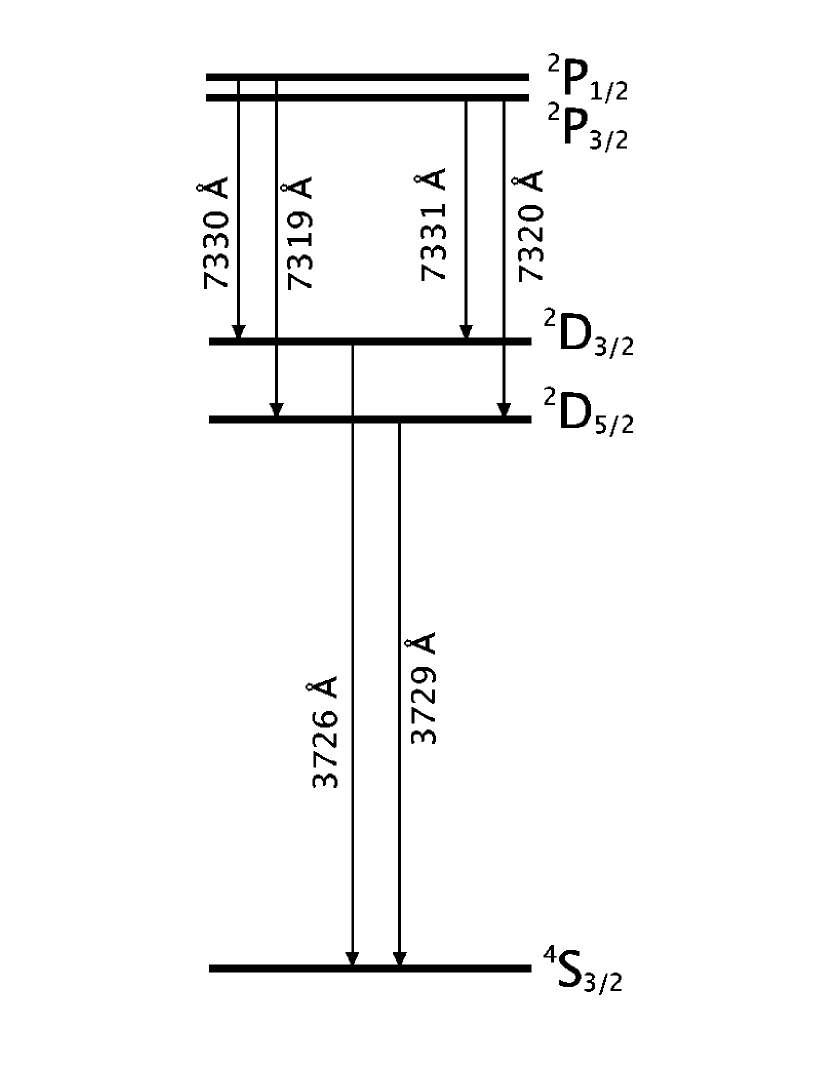
Figure 1: Grotrian diagram of O ii ground configuration energy level transitions (not to scale). Wavelengths are approximate air values.

In this paper we determine the four energies which describe the separation of the five ground configuration energy levels of O ii shown in Figure 1, through analysis of observations of the visible forbidden transitions. Being forbidden transitions, these are weak and not accessible in the laboratory. The ground configuration levels can be determined from laboratory data on permitted ultraviolet transitions from higher states, but in practice the uncertainties in the derived energy levels are larger than those obtained from the nebular visible transitions. Thus the published compilations of data on these energy levels (Eriksson 1988; Martin, Kaufman & Musgrove 1993) rely heavily on the pioneering work of Bowen (1960) and de Robertis, Osterbrock, & McKee (1985) on planetary nebulae (see Table 1). Our analysis of new data improves upon these energies and provides a discussion of the uncertainties.

Bowen (1960) observed the two blue [O ii] lines in seven bright planetary nebulae (a total of sixteen photographic plates) and the four red [O ii] lines (blended into two lines) in one nebula (three separate plates). The O⁺ gas of the planetary nebulae was assumed to have an average bulk velocity identical to the measured velocity of the H⁺ gas (the H⁺ energy levels being well known). The observed [O ii] wavelengths adjusted to this velocity give absolute wavenumbers for the energy level differences for the transitions. These early data resolved the ²D term into its two $J$ components, but were not able to determine the splitting of the ²P term. The latter splitting was determined in de Robertis et al. (1985) using high-resolution digital spectra of the four red lines in one bright planetary nebula (NGC 7027). As can be appreciated from Figure 1, the red transitions ending on a common lower level constrain the splitting of the ²P term while the transitions from a common upper level constrain the splitting of the ²D term, independently of the blue data. de Robertis et al. (1985) found a value for the latter splitting somewhat different than that found by Bowen. Since absolute velocities or wavenumbers were not measured, de Robertis et al. (1985) calculated the ²D–²P separation by assuming that the $\lambda$7319/$\lambda$7320 line blend measured by Bowen (1960) was actually a measure of the stronger $\lambda$7320 line, and that Bowen (1960)’s roughly symmetric $\lambda$7330/$\lambda$7331 blend was a measure of this line pair’s average.

We show that H ii regions can also be used to determine the energy levels of O ii. With high-resolution echelle spectroscopy of the Orion nebula (resolving all red and blue lines), we are able to measure not only the splitting of both the ²P and ²D terms but also the separation between these two split terms. The observations are described in § 3 and the full analysis, including uncertainties, in § 4. But first we update Bowen’s work by analysis of more recent digital data on 23 planetary nebulae (§ 2). This provides important insight into the method of analysis of the full Orion data and also provides improved values of the two energies constrained by the blue lines à la Bowen.

We conclude by comparing our results with recent work by Sharpee et al. (2004).

2 Bowen revisited

Using a coudé spectrograph on the Hale telescope, Bowen (1955) observed the blue spectra of seven planetary nebulae photographically. Since the introduction of the Hamilton Echelle Spectrograph in 1987 (Vogt, 1987), high-resolution spectra of (at least) 24 planetary nebulae spectra have been published, the relevant data for our purposes being the line lists with accurately tabulated wavelengths. (One nebula, NGC 6818, had to be discarded because of a grossly discrepant wavelength – we suspect a typographical error.) These new spectra resolve the blue lines but not the red pairs of lines.

Following Bowen we therefore have two lines to constrain two energies. But there is an important requirement: we need to know the velocity of the line-producing gas and any uncertainty ($\delta v_{\mathrm{O^{+}}}$) will have predictable consequences. For example, if one uses the 3729 Å line to find the energy difference for this transition, $E_{{}^{4}\mathrm{S}_{3/2}-^{2}\mathrm{D}_{5/2}}$ (note the convention of an “upwards” transition), because of this degeneracy the Doppler effect gives an uncertainty

$$\delta E_{{}^{4}\mathrm{S}_{3/2}-^{2}\mathrm{D}_{5/2}}=0.0895\delta v_{\mathrm{O^{+}}},$$ (1)

where throughout this paper energies are in units of cm^-1 and velocities in km s^-1. Looking ahead to the red data,

$$\delta E_{{}^{2}\mathrm{D}_{3/2}-^{2}\mathrm{P}_{3/2}}=0.0455\delta v_{\mathrm{O^{+}}}=0.50865\delta E_{{}^{4}\mathrm{S}_{3/2}-^{2}\mathrm{D}_{5/2}},$$ (2)

but note that the smaller splittings $E_{{}^{2}\mathrm{D}_{5/2}-^{2}\mathrm{D}_{3/2}}$ and $E_{{}^{2}\mathrm{P}_{3/2}-^{2}\mathrm{P}_{1/2}}$ are much less susceptible to any uncertainty in the velocity.

In Bowen’s work, permitted lines of H⁺ and He⁺ gas set the rest-frame velocity and similarly here all wavelengths for all 23 planetary nebulae are first put into such a reference frame with H⁺ at rest. As tabulated by the authors, the planetary nebulae wavelengths have in fact already been corrected for the previously-known systemic velocity of the whole nebula, but nevertheless we find from the data that the H⁺ is apparently not quite at rest. This is either because the systemic velocity used was only approximate, or because for the slit positions observed the mean velocity of the H⁺ gas is not identical to that averaged over the nebula, which would not be surprising given incomplete coverage of an expanding nebula. To define the H⁺ frame for each nebula, we used the eight or nine unblended H i lines (H16 to H$\delta$) near the blue [O ii] lines, these all being contained in the same echelle spectrum. The corresponding blue wavelengths are given in Table 2.

The measured velocity of O⁺ is not necessarily the same as that of H⁺ because of the ionization structure and expansion that exist in the nebula and the fact that the slit does not usually cover the entire nebula. Bowen’s approach was to average results over several nebulae, since on average the two velocities should be equal. Given data on 23 nebulae, we can improve upon this iteratively as explained below.

Our analysis is basically to develop a parameterized model, and then optimize the parameters by non-linear least squares to match predicted wavelengths, in air, with the wavelengths tabulated. The parameters of the model are the energies and any velocity offsets ($v_{\mathrm{O}^{+}}$) deemed necessary. (Toward this end, deviations of observed wavelengths from the model predictions are expressed in terms of velocity.) The energies can be taken as the successive energy differences, four independent values in the full model, or simply the energies of the four upper levels. Even with the first of these two options there is covariance in the resulting solution, since four of the six energy transitions (corresponding to four of the six available wavelengths) couple the independent successive energy differences. The “model uncertainties” from the goodness of fit to the model are the 68.3% confidence intervals for one-dimensional marginal distributions for each of the parameters.

Let us return to the blue lines, for which we have 46 measured wavelengths for 23 planetary nebulae. As energy parameters, we used $E_{{}^{4}\mathrm{S}_{3/2}-^{2}\mathrm{D}_{5/2}}$ and $E_{{}^{2}\mathrm{D}_{5/2}-^{2}\mathrm{D}_{3/2}}$. In the initial model we went to the extreme of introducing 23 velocity offsets. This precludes determining $E_{{}^{4}\mathrm{S}_{3/2}-^{2}\mathrm{D}_{5/2}}$ and we find $E_{{}^{2}\mathrm{D}_{5/2}-^{2}\mathrm{D}_{3/2}}=19.79\pm 0.05$. For each nebula the two velocity residuals (from the two wavelength residuals) are of equal magnitude (denoted $\sigma_{int}$) with opposite signs, indicating that relative to the model the two lines are too close together or too widely separated. Overall the rms velocity residual was 0.96 km s^-1. Those nebulae with considerably larger rms values can be judged to have data of lower quality; i.e., even with the luxury of the maximal number of parameters, the data are still not going to be well matched by the model. Two nebulae with residuals greater than 2.4 km s^-1 have been assigned weight 0.25 (in the calculation of $\chi^{2}$) while another four with residuals greater than 1.2 km s^-1 have been assigned weight 0.5. No bias is introduced in subsequent calculations of the splitting $E_{{}^{2}\mathrm{D}_{5/2}-^{2}\mathrm{D}_{3/2}}$ since equal numbers of “too close” and “too separated” cases are involved; now $E_{{}^{2}\mathrm{D}_{5/2}-^{2}\mathrm{D}_{3/2}}=19.79\pm 0.04$. The weighted rms residual is 0.71 km s^-1 and no subsequent model, with fewer parameters, can improve upon this.

The next model goes to the other extreme, fitting only the two energy differences, finding $E_{{}^{4}\mathrm{S}_{3/2}-^{2}\mathrm{D}_{5/2}}=26810.68\pm 0.13$ and $E_{{}^{2}\mathrm{D}_{5/2}-^{2}\mathrm{D}_{3/2}}=19.79\pm 0.18$. The latter energy difference is still close to that in the initial model, but is determined with less confidence because the two-parameter model fits the data less well. The rms velocity residual is 6.7 km s^-1, much larger than suggested by our assessment of the data quality, and so clearly indicating a less than optimal model.

Thus our goal was to improve the model iteratively by adding a minimal number of parameters $v_{\mathrm{O}^{+}}$, for a subset of the nebulae, expecting a significant reduction in $\chi^{2}$ per degree of freedom. We identified seven nebulae for which the residuals exceeded 6.7 km s^-1 and also $3\sigma_{int}<6.7$ km s^-1 and for these included a velocity offset parameter. This produced a markedly improved model with an rms residual of 1.9 km s^-1 and $E_{{}^{4}\mathrm{S}_{3/2}-^{2}\mathrm{D}_{5/2}}=26810.77\pm 0.04$ and $E_{{}^{2}\mathrm{D}_{5/2}-^{2}\mathrm{D}_{3/2}}=19.79\pm 0.06$. Repeating this process with the new rms identifies eight more nebulae which would benefit from velocity offsets, for a total of 15 of the 23 nebulae. This iteration reduces the rms velocity residual to 0.82 km s^-1; this is now comparable to the above estimate of the quality of the data, indicating that adding further parameters would not be justified. $E_{{}^{4}\mathrm{S}_{3/2}-^{2}\mathrm{D}_{5/2}}=26810.77\pm 0.03$ and $E_{{}^{2}\mathrm{D}_{5/2}-^{2}\mathrm{D}_{3/2}}=19.79\pm 0.03$ – the only difference with respect to the previous iteration being a lowering of the error (confidence interval). It is important to acknowledge that there is a systematic error in $E_{{}^{4}\mathrm{S}_{3/2}-^{2}\mathrm{D}_{5/2}}$ of order 0.03 cm^-1 because the introduction of parameters $v_{\mathrm{O}^{+}}$, while hopefully unbiased, is still subjective. Such systematic errors are recorded separately in Table 1 to distinguish them from confidence intervals.

The energies determined are close to those given by Bowen, but significantly different than those derived by de Robertis et al. (1985) – refer to Table 1.

3 Observations of the Orion Nebula

High-resolution echelle spectra were obtained over the course of two nights in 1997 (5100-7485 Å) and 1998 (3510-5940 Å) with the CTIO 4-m Blanco telescope (refer to Baldwin et al. (2000) for details). Three different lines of sight were observed, referred to as 1SW, x2 (Baldwin et al., 1996; Rubin et al., 1997) and 37W (Baldwin et al., 1991). To extract the information on individual lines, in particular the wavelength, the data were modeled with a Gaussian (three parameters: central wavelength, FWHM, area) and a linear baseline (two further parameters). The rest-frame velocity of the H⁺ gas along each line of sight was determined from the six strongest unblended H i Balmer lines.

All six [O ii] forbidden lines are seen with good signal to noise in these spectra. Data for 1SW are shown in Figure 2. The pairs of [O ii] red lines were slightly blended and so were analysed using a double Gaussian fit. The results of our line fitting are summarized in Table 3. All line profiles are similar as seen in the matching FWHM and directly from the spectra in Figure 2.

For the common upper level line pairs $\lambda$7320/$\lambda$7331 and $\lambda$7319/$\lambda$7330 the line strength ratios can be predicted directly from the transition probabilities (Zeippen, 1987; Wiese et al., 1996), offering an independent check of one aspect of the fits. Results are presented in Table 4. There is reasonable agreement between the theory and the observations. The sole anomaly, seen in the $\lambda$7319/$\lambda$7330 ratio in the x2 line-of-sight, arises because of a velocity-shifted component from a photoionized Herbig-Haro shock (Blagrave & Martin, 2004a) that has 2-4$\%$ of the nebular [O ii] flux. The nebular $\lambda$7330 and $\lambda$7319 lines are contaminated by the velocity-shifted components of $\lambda$7331 and $\lambda$7320, respectively. A higher relative contamination from the stronger of these two lines, $\lambda$7320, results in a higher $\lambda$7319/$\lambda$7330 ratio.

All four [O ii] red lines are found in the same echelle order of a single exposure, unlike in the data of de Robertis et al. (1985) where the $\lambda$7319/$\lambda$7320 and $\lambda$7330/$\lambda$7331 line pairs were obtained in two separate spectra. Measuring the ²P energy splitting $E_{{}^{2}\mathrm{P}_{3/2}-^{2}\mathrm{P}_{1/2}}$ depends on the wavelength difference within each of the line pairs and so the results in de Robertis et al. (1985) should be accurate. On the other hand, the splitting of the ²D term $E_{{}^{2}\mathrm{D}_{5/2}-^{2}\mathrm{D}_{3/2}}$ depends on the wavelength difference between the pairs and so our single spectrum containing both line pairs, with only a single wavelength calibration in the same echelle order, should yield a more accurate result.

All lines produced by the same ionized species should have the same velocity. However, using the current published energy levels and derived rest wavelengths in air (Eriksson, 1987; Martin et al., 1993) together with our observed wavelengths, we obtain O⁺ velocities that are grossly inconsistent, well beyond the uncertainties propagated from the measurement errors of the observed wavelengths (see Table 5). In particular, there is no explanation why lines in the same wavelength region and originating from a common upper level (²P_1/2 or ²P_3/2) should yield significantly different velocities, as is observed to be the case in columns 7 and 8 of Table 5; at the very least, there is a problem with the splitting $E_{{}^{2}\mathrm{D}_{5/2}-^{2}\mathrm{D}_{3/2}}$. The consistency of the data for the three lines of sights, and the lack of agreement of the velocities from all of the lines, points to inaccurate [O ii] rest wavelengths arising from poorly determined ground configuration energy levels, including the separations $E_{{}^{4}\mathrm{S}_{3/2}-^{2}\mathrm{D}_{5/2}}$ and $E_{{}^{2}\mathrm{D}_{3/2}-^{2}\mathrm{P}_{3/2}}$. This was the original motivation for this paper.

4 Constraining the Energy Levels with the Orion Nebula Data

With a set of six accurate wavelengths, for each of three lines-of-sight (1SW, x2, and 37W), it is possible to obtain the energies of the four excited levels in the ground configuration of O ii (Fig. 1); the problem is over-constrained. However, as encountered in the analysis of planetary nebula spectra in § 2, there is the possibility of an unknown velocity offset of the O⁺ gas for each position observed. But even with an extra velocity offset parameter $v_{\mathrm{O}^{+}}$ for each position, the problem is still over-constrained (even for a single position) and thus amenable to modeling and least-squares optimization.

As with the planetary nebulae, there is a Doppler-related degeneracy to be resolved as well, through independent constraints on $v_{\mathrm{O}^{+}}$. We show how this is possible in Orion, it not being sufficient to assume that on average, over many positions, the velocities of the O⁺ gas and H⁺ gas are identical (in which case $\left<v_{\mathrm{O}^{+}}\right>=0$).

The Orion nebula can be represented by a blister model where gas is accelerating toward the ionizing star and the observer away from the background molecular cloud (Balick et al., 1974). Because of ionization stratification in this accelerating flow, the velocity is correlated with the ionization potential (I.P.): gas that is more highly ionized is more blue shifted (has more negative velocity). This is observed; see, e.g., Baldwin et al. (2000). Figure 3, plotting velocity against the emitting species’ I.P., summarizes this effect for our observations of many lines of many different ions for the three lines of sight. Models of the nebula (Baldwin et al., 2000) show that the O⁺ zone is relatively narrow (see their Figure 4) and so there should be a well defined velocity. From the trend seen in Figure 3, the expected value for $v_{\mathrm{O}^{+}}$, at I.P. 35 eV for O⁺, lies between 0 and 5 km s^-1, set in part by the [S iii] (I.P. = 34.79 eV) velocities at similar ionization potential. Plotting the results in columns 7 and 8 of Table 5 in Figure 3 would clearly reveal their discrepancy, again pointing to a problem with the energy levels. The velocities from our new O⁺ model clearly satisfy the general constraint set by the surrounding lines.

As in the analysis of the planetary nebula data, our examination of the Orion nebula data is rooted in a model of the energy levels, used to predict the air wavelengths. In this case we set $E_{{}^{4}\mathrm{S}_{3/2}-^{2}\mathrm{D}_{5/2}}=26810.77$, the result already found in § 2. The remaining analysis is then a non-linear least squares fit (unweighted), using six parameters in the model: the other three energy differences, and the three velocities $v_{\mathrm{O}^{+}}$. This model produces rms energy-difference residuals of only 0.4 km s^-1. Line by line and position by position, this model gives the velocities listed in column 9 of Table 5; these are clearly now quite consistent with one another.

This choice of $E_{{}^{4}\mathrm{S}_{3/2}-^{2}\mathrm{D}_{5/2}}$ produces $v_{\mathrm{O}^{+}}$ equal to $4.0\pm 0.3$ km s^-1, $4.1\pm 0.3$ km s^-1, and $1.4\pm 0.3$ km s^-1 for 1SW, x2, and 37W, respectively (because of changes in geometry from one line-of-sight to the next, these velocities need not be identical). It turns out that these fall in line with the trend in Figure 3 and so no optimization was carried out on this energy difference.

Recall however, that if a slight change were made in this energy, $v_{\mathrm{O}^{+}}$ would respond according to equation 1. Thus the model uncertainty $\delta E_{{}^{4}\mathrm{S}_{3/2}-^{2}\mathrm{D}_{5/2}}$ from the planetary nebulae analysis, $\pm 0.03$ cm^-1, results in $\delta v_{\mathrm{O}^{+}}=0.34$ km s^-1. This is of the same order as the model fitting uncertainties for the Orion data. In principle, one might start by determining $v_{\mathrm{O}^{+}}$ and its uncertainty from interpolation in Figure 3 and work backwards to $E_{{}^{4}\mathrm{S}_{3/2}-^{2}\mathrm{D}_{5/2}}$ and its uncertainty. Given the consistency, we adopt the tighter constraint found independently in § 2. This will propagate as a systematic uncertainty through to the other energies (see equation 2).

Uncertainties in $v_{\mathrm{O}^{+}}$ have the same effect as uncertainties in the wavelength calibration, which we deduce is accurate to 0.5 km/s, consistent with the scatter of individual blue H⁺ line velocities about the mean. Thus, for the remainder of the Orion analysis, we adopt $\delta v_{\mathrm{O}^{+}}=0.5$ km s^-1, noting that this subsumes errors in the wavelength calibration of the blue lines. For the red lines there is an additional systematic error of order 0.15 km s^-1 relating to the alignment of the separate red and blue echelle spectra into the same velocity/wavelength system. The next issue is the accuracy of the wavelength calibration for individual lines. To assess this, we note that there are numerous lines that are duplicated in neighbouring echelle orders of the same spectrum. By comparing the duplicate measurements of these lines’ wavelengths, we find a residual characteristic order-to-order difference of 0.65 km s^-1, independent of measurement uncertainty. In practice, we feel that measurements of the red [O ii] lines, which all appear in the centre of an order, have a systematic uncertainty of less than half this, $\sim 0.3$ km s^-1. Taken all together, the combined systematic error is of order 0.7 km s^-1, which corresponds to $\delta E_{{}^{2}\mathrm{D}_{3/2}-^{2}\mathrm{P}_{3/2}}=0.03$. Therefore, the separation $E_{{}^{2}\mathrm{D}_{3/2}-^{2}\mathrm{P}_{3/2}}$ is properly quoted as $13637.34\pm 0.01\pm 0.03$. This is significantly different than what has been previously adopted (see Table 1).

On the other hand, for the small splittings, the systematic effects are tiny compared to the model uncertainties, and so are listed below as 0.00. As anticipated, we find that the value of the splitting $E_{{}^{2}\mathrm{P}_{3/2}-^{2}\mathrm{P}_{1/2}}$ of the ²P term, $2.02\pm 0.01\pm 0.00$, is in close agreement with that found by de Robertis et al. (1985), $2.00\pm 0.03$ (largely adopted by Eriksson (1987) and Martin et al. (1993)).

The splitting $E_{{}^{2}\mathrm{D}_{5/2}-^{2}\mathrm{D}_{3/2}}$ of the ²D term is $19.80\pm 0.01\pm 0.00$, closely consistent with the value $19.79\pm 0.03\pm 0.03$ obtained in § 2 from only the blue lines of planetary nebulae. We conclude that the splitting of the ²D term should be revised from the value $20.1\pm 0.1$ found by de Robertis et al. (1985) and (largely) adopted by Eriksson (1987) and Martin et al. (1993).

These energy differences allow us to calculate the energies of all four energy levels (see Table 1). The model was rewritten with these energies as the parameters in order to track the effects of covariant changes in this non-linear model of the air wavelengths, and thus provide the appropriate one-dimensional marginal confidence intervals reported in Table 1. The errors reported are again the model fitting uncertainty and the systematic error. The latter reflects the propagation of the error in $E_{{}^{4}\mathrm{S}_{3/2}-^{2}\mathrm{D}_{5/2}}$ plus the systematic error in $E_{{}^{2}\mathrm{D}_{3/2}-^{2}\mathrm{P}_{3/2}}$ for the highest two energies

These energy levels allow for the calculation of the air wavelengths of lines in the UV in addition to those in Table 5. From $E_{{}^{4}\mathrm{S}_{3/2}-^{2}\mathrm{P}_{3/2}}$ $E_{{}^{4}\mathrm{S}_{3/2}-^{2}\mathrm{P}_{1/2}}$, we calculate $\lambda 2470.347\pm 0.001\pm 0.003$ and $\lambda 2470.223\pm 0.001\pm 0.003$, respectively.

Because of the presence of systematic errors, the above analysis was carried out with equal weights for all lines. However, we have repeated the analysis using a weighted fit based on the uncertainties found in measuring each line. $E_{{}^{2}\mathrm{D}_{5/2}-^{2}\mathrm{D}_{3/2}}$ increased by only 0.001, $E_{{}^{2}\mathrm{D}_{3/2}-^{2}\mathrm{P}_{3/2}}$ decreased by 0.015 (well within the systematic uncertainty) and $E_{{}^{2}\mathrm{P}_{3/2}-^{2}\mathrm{P}_{1/2}}$ increased by 0.007 (recorded in Table 1 as 0.01 systematic uncertainty).

5 Comparison to Recent Work of Sharpee et al.

Sharpee et al. (2004) have observed the four red lines ($\lambda\lambda$7319, 7320, 7330, 7331 Å) in sky spectra using the high-resolution echelle spectrograph (HIRES) on Keck I. In their determination of the O ii $2p^{3}$ energy levels, they also make use of data-sets from nebulae (Bowen, 1960; de Robertis et al., 1985; Baldwin et al., 2000; Sharpee et al., 2003). The nebular data are given lesser weights (0.018, 0.16, 1.00, 1.00, respectively) than the HIRES data-set (10.00). Velocity corrections for data-sets of three nebulae (de Robertis et al., 1985; Baldwin et al., 2000; Sharpee et al., 2003) were found using a weighted least-squares analysis similar to what was done in § 2; Bowen (1960) is an average of multiple nebulae and was assumed to have $\left<v_{\mathrm{O}^{+}}\right>=0$. From these five data-sets, they obtain splittings of $19.810\pm 0.006$ and $2.010\pm 0.005$ for the ²D and ²P terms, respectively – both in excellent agreement with our results.

The ²D${}_{3/2}-^{2}$P_3/2 separation, $13637.403\pm 0.004$, is quoted here with their 1$\sigma$ model fitting uncertainty. Even though for the HIRES data one knows $v_{\mathrm{O}^{+}}=0$, there is still a systematic uncertainty because of the wavelength calibration which was accomplished through the OH Meinel band. From their stated “statistical scatter” of 0.5 km s^-1 we judge that the systematic error in $E_{{}^{2}\mathrm{D}_{3/2}-^{2}\mathrm{P}_{3/2}}$ is no larger than 0.023 cm^-1 (see equation 2), and 0.012 Å in the wavelengths of the red lines. Based on the model-fitting uncertainties alone, our value $13637.34\pm 0.01\pm 0.03$ might seem significantly different, but the values are in fact consistent when one accounts for the systematic uncertainties. If we adopted the Sharpee et al. (2004) value of $E_{{}^{2}\mathrm{D}_{3/2}-^{2}\mathrm{P}_{3/2}}$, the velocities in Table 5 would be more consistent for 37W, but correspondingly less consistent for the other two positions.

To complete their set of O ii $2p^{3}$ energy levels, the blue lines from three nebulae (Bowen, 1960; Baldwin et al., 2000; Sharpee et al., 2004) were used to deduce $E_{{}^{4}\mathrm{S}_{3/2}-^{2}\mathrm{D}_{5/2}}=26810.76\pm 0.08$ (no systematic error was estimated). This energy difference compares well with our result using 23 planetary nebulae, $26810.77\pm 0.03\pm 0.03$.

The UV wavelengths depend on both $E_{{}^{4}\mathrm{S}_{3/2}-^{2}\mathrm{D}_{5/2}}$ and $E_{{}^{2}\mathrm{D}_{3/2}-^{2}\mathrm{P}_{3/2}}$, and so the Sharpee et al. (2004) values $\lambda 2470.343\pm 0.005$ and $\lambda 2470.220\pm 0.005$ are consistent with ours though slightly less accurate.

6 Conclusions

From a detailed analysis of Orion nebula and planetary nebulae data, we find new energies for the ground configuration. Both model-fitting uncertainties and systematic uncertainties are presented. This work confirms the utility of astrophysical measurements in determining accurate energies for the O ii $2p^{3}$ ground configuration. As a by-product, we determine a revised set of air wavelengths of the [O ii] visible lines (see Table 5) and the UV lines (see § 4). As Sharpee et al. (2004) point out, there are revisions required in the standard NIST values.

Using these revised wavelengths, it is now possible to constrain the velocities of all three oxygen zones (O⁰,O⁺,O⁺⁺), and in turn, the spatial and physical origin of oxygen permitted lines can be inferred (Blagrave & Martin, 2004b).

Figure 2: Gaussian profile fit of all six visible O ii lines (1SW). The dark solid line represents the observed line profile and the lighter dashed line represents the Gaussian fit. The wavelength has been adjusted to the rest-frame velocity of the H⁺ gas. Refer to Table 3 for reddening-corrected fluxes and the results of the line-fitting.

Figure 3: Gas velocity as a function of the emitting species’ ionization potential. The three lines-of-sight have been offset in the x-direction to properly show the standard deviations about the mean velocities for each line-of-sight. The ionization potentials of O⁰ and O⁺⁺ are 13.6181 eV and 54.934 eV, respectively. O⁺ ionization potential is 35 eV.

Table 1: O ii ground configuration energy levels (cm^-1)

Designation	Bowen	De Robertis	Level	Eriksson	Martin et al.	This Work	Level
	(1955)	et al. (1985)	Difference	(1987)	(1993)		Difference
4S3/2	0.0	0.0		0.00	0.00	0.00
2D5/2	26810.7	26810.5	26810.5	26810.52	26810.55	$26810.77\pm 0.03\pm 0.03$	$26810.77\pm 0.03\pm 0.03$
2D3/2	26830.5	26830.6	$20.1\pm 0.1$	26830.57	26830.57	$26830.57\pm 0.01\pm 0.03$	$19.80\pm 0.01\pm 0.00$
2P3/2		40468.1	13637.5	40467.69	40468.01	$40467.91\pm 0.02\pm 0.05$	$13637.34\pm 0.01\pm 0.03$
2P1/2	40468.3	40470.1	$2.00\pm 0.03$	40469.69	40470.00	$40469.93\pm 0.02\pm 0.05$	$2.02\pm 0.01\pm 0.01$

Table 2: Determination of ²D_5/2 energy from planetary nebulae data

Nebula	4S3/2-2D3/2 (Å)	4S3/2-2D5/2 (Å)	Weight	Reference
NGC 2440	3726.00	3728.69	0.25	Hyung & Aller (1998)
NGC 6543	3726.06	3728.81	1.0	Hyung et al. (2000)
NGC 6567	3726.25	3728.97	0.5	Hyung et al. (1993)
NGC 6572	3726.01	3728.76	1.0	Hyung et al. (1994b)
NGC 6741	3726.15	3728.90	1.0	Hyung & Aller (1997a)
NGC 6790	3726.00	3728.74	1.0	Aller et al. (1996)
NGC 6818	3726.32	3728.79	0.0	Hyung et al. (1999b)
NGC 6884	3726.02	3728.80	0.5	Hyung et al. (1997)
NGC 6886	3726.05	3728.78	1.0	Hyung et al. (1995)
NGC 7009major	3725.97	3728.71	1.0	Hyung & Aller (1995b)
NGC 7009minor	3726.14	3728.95	0.25	Hyung & Aller (1995a)
NGC 7662	3725.94	3728.69	1.0	Hyung & Aller (1997b)
IC 351	3726.04	3728.81	1.0	Feibelman et al. (1996)
IC 418	3726.04	3728.80	1.0	Hyung et al. (1994a)
IC 2149	3725.99	3728.76	1.0	Feibelman et al. (1994)
IC 2165	3726.18	3728.96	0.5	Hyung (1994)
IC 4634	3726.27	3729.02	1.0	Hyung et al. (1999a)
IC 4846	3726.17	3728.93	1.0	Hyung et al. (2001c)
IC 4997	3725.97	3728.71	1.0	Hyung et al. (1994c)
IC 5117	3726.03	3728.75	0.5	Hyung et al. (2001a)
IC 5217	3726.04	3728.77	1.0	Hyung et al. (2001b)
BD +30 3639	3726.01	3728.77	1.0	Aller & Hyung (1995)
Hubble 12	3726.04	3728.80	1.0	Hyung & Aller (1996)
Hu 1-2	3726.07	3728.83	1.0	Pottasch et al. (2003)

Table 3: Best-fit line parameters for visible wavelength transitions.

Transition	Position	Measured Wavelength (Å)	FWHM (km s-1)	Reddening corrected line strength
				($10^{-13}$ erg s-1 cm-2)
4S${}_{3/2}-^{2}$D3/2	1SW	$3726.072\pm 0.001$	$16.8\pm 0.2$	$426\pm 6$
	x2	$3726.078\pm 0.001$	$18.0\pm 0.3$	$273\pm 4$
	37W	$3726.060\pm 0.002$	$15.3\pm 0.3$	$466\pm 9$
4S${}_{3/2}-^{2}$D5/2	1SW	$3728.824\pm 0.001$	$17.3\pm 0.2$	$188\pm 2$
	x2	$3728.829\pm 0.002$	$19.1\pm 0.2$	$138\pm 2$
	37W	$3728.811\pm 0.002$	$15.7\pm 0.3$	$213\pm 4$
2D${}_{5/2}-^{2}$P1/2	1SW	$7319.173\pm 0.006$	$18.0\pm 0.6$	$14.7\pm 0.5$
	x2	$7319.178\pm 0.008$	$21.3\pm 0.8$	$6.9\pm 0.2$
	37W	$7319.099\pm 0.011$	$16.9\pm 1.1$	$10.8\pm 0.6$
2D${}_{5/2}-^{2}$P3/2	1SW	$7320.253\pm 0.002$	$17.5\pm 0.2$	$42.6\pm 0.5$
	x2	$7320.250\pm 0.003$	$19.3\pm 0.3$	$17.1\pm 0.2$
	37W	$7320.181\pm 0.004$	$16.9\pm 0.4$	$32.0\pm 0.6$
2D${}_{3/2}-^{2}$P1/2	1SW	$7329.787\pm 0.004$	$17.9\pm 0.4$	$21.1\pm 0.4$
	x2	$7329.798\pm 0.006$	$23.4\pm 0.6$	$8.6\pm 0.2$
	37W	$7329.725\pm 0.005$	$16.0\pm 0.5$	$16.6\pm 0.4$
2D${}_{3/2}-^{2}$P3/2	1SW	$7330.886\pm 0.003$	$18.1\pm 0.3$	$24.0\pm 0.4$
	x2	$7330.885\pm 0.004$	$19.8\pm 0.4$	$9.5\pm 0.2$
	37W	$7330.818\pm 0.005$	$17.7\pm 0.5$	$18.2\pm 0.5$

Table 4: Comparison between observed and predicted line ratios as determined from transition probabilities, $A_{ij}$.

Transition	1SW		x2		37W		Zeippen (1987)		Wiese et al. (1996)
	Flux	Ratio	Flux	Ratio	Flux	Ratio	$A_{ij}$	Ratio	$A_{ij}$	Ratio
2D${}_{5/2}-^{2}$P1/2 ($\lambda$7319)	$14.7\pm 0.5$		$6.9\pm 0.2$		$10.8\pm 0.6$		0.0563		$0.0519\pm 0.0052$
2D${}_{3/2}-^{2}$P1/2 ($\lambda$7330)	$21.1\pm 0.4$	$0.70\pm 0.03$	$8.6\pm 0.2$	$0.80\pm 0.03$	$16.6\pm 0.4$	$0.65\pm 0.04$	0.0941	0.598	$0.0867\pm 0.0087$	$0.599\pm 0.085$
2D${}_{5/2}-^{2}$P3/2 ($\lambda$7320)	$42.6\pm 0.5$		$17.1\pm 0.2$		$32.0\pm 0.6$		0.1067		$0.0991\pm 0.0099$
2D${}_{3/2}-^{2}$P3/2 ($\lambda$7331)	$24.0\pm 0.4$	$1.77\pm 0.04$	$9.5\pm 0.2$	$1.80\pm 0.04$	$18.2\pm 0.5$	$1.76\pm 0.06$	0.0580	1.84	$0.0534\pm 0.0053$	$1.86\pm 0.26$

Table 5: Line velocities in Orion using recent wavelength tabulations.

	Air $\lambda$ (Å)					Velocity  (km s-1)
Transition	Martin	Eriksson	This work	Position	Observed $\lambda$ (Å)	Martin	Eriksson	This work
(1)	(2)	(3)	(4)	(5)	(6)	(7)	(8)	(9)
4S${}_{3/2}-^{2}$D3/2	3726.032	3726.032	3726.032	1SW	3726.072	$3.2\pm 0.1$	$3.2\pm 0.1$	$3.2\pm 0.1$
			$\pm 0.001$	x2	3726.078	$3.7\pm 0.1$	$3.7\pm 0.1$	$3.7\pm 0.1$
			$\pm 0.004$	37W	3726.060	$2.3\pm 0.2$	$2.3\pm 0.2$	$2.3\pm 0.2$
4S${}_{3/2}-^{2}$D5/2	3728.815	3728.819	3728.784	1SW	3728.824	$0.7\pm 0.1$	$0.4\pm 0.1$	$3.2\pm 0.1$
			$\pm 0.004$	x2	3728.829	$1.1\pm 0.2$	$0.8\pm 0.2$	$3.6\pm 0.2$
			$\pm 0.004$	37W	3728.811	$-0.3\pm 0.2$	$-0.6\pm 0.2$	$2.2\pm 0.2$
2D${}_{5/2}-^{2}$P1/2	7318.92	7319.07	7319.073	1SW	7319.173	$10.4\pm 0.2$	$4.2\pm 0.2$	$4.1\pm 0.2$
			$\pm 0.009$	x2	7319.178	$10.6\pm 0.3$	$4.4\pm 0.3$	$4.3\pm 0.3$
			$\pm 0.012$	37W	7319.099	$7.3\pm 0.5$	$1.2\pm 0.5$	$1.1\pm 0.5$
2D${}_{5/2}-^{2}$P3/2	7319.99	7320.14	7320.157	1SW	7320.253	$10.8\pm 0.1$	$4.6\pm 0.1$	$3.9\pm 0.1$
			$\pm 0.009$	x2	7320.250	$10.6\pm 0.1$	$4.5\pm 0.1$	$3.8\pm 0.1$
			$\pm 0.012$	37W	7320.181	$7.8\pm 0.2$	$1.7\pm 0.2$	$1.0\pm 0.2$
2D${}_{3/2}-^{2}$P1/2	7329.67	7329.83	7329.699	1SW	7329.787	$4.8\pm 0.1$	$-1.8\pm 0.1$	$3.6\pm 0.1$
			$\pm 0.005$	x2	7329.798	$5.2\pm 0.2$	$-1.3\pm 0.2$	$4.0\pm 0.2$
			$\pm 0.012$	37W	7329.725	$2.2\pm 0.2$	$-4.3\pm 0.2$	$1.1\pm 0.2$
2D${}_{3/2}-^{2}$P3/2	7330.73	7330.91	7330.786	1SW	7330.886	$6.4\pm 0.1$	$-1.0\pm 0.1$	$4.1\pm 0.1$
			$\pm 0.005$	x2	7330.885	$6.3\pm 0.2$	$-1.0\pm 0.2$	$4.0\pm 0.2$
			$\pm 0.012$	37W	7330.818	$3.6\pm 0.2$	$-3.8\pm 0.2$	$1.3\pm 0.2$

References

- Aller & Hyung (1995) Aller, L. H. & Hyung, S. 1995, MNRAS, 276, 1101
- Aller et al. (1996) Aller, L. H., Hyung, S., & Feibelman, W. A. 1996, PASP, 108, 488
- Baldwin et al. (1996) Baldwin, J. A., Crotts, A., Dufour, R. J., Ferland, G. J., Heathcote, S., Hester, J. J., Korista, K. T., Martin, P. G., O’Dell, C. R., Rubin, R. H., Tielens, A. G. G. M., Verner, D. A., Verner, E. M., Walter, D. K., & Wen, Z. 1996, ApJ, 468, L115
- Baldwin et al. (1991) Baldwin, J. A., Ferland, G. J., Martin, P. G., Corbin, M. R., Cota, S. A., Peterson, B. M., & Slettebak, A. 1991, ApJ, 374, 580
- Baldwin et al. (2000) Baldwin, J. A., Verner, E. M., Verner, D. A., Ferland, G. J., Martin, P. G., Korista, K. T., & Rubin, R. H. 2000, ApJS, 129, 229
- Balick et al. (1974) Balick, B., Gammon, R. H., & Hjellming, R. M. 1974, PASP, 86, 616
- Blagrave & Martin (2004a) Blagrave, K. P. M. & Martin, P. G. 2004a, in preparation
- Blagrave & Martin (2004b) —. 2004b, in preparation
- Bowen (1955) Bowen, I. S. 1955, ApJ, 121, 306
- Bowen (1960) —. 1960, ApJ, 132, 1
- de Robertis et al. (1985) de Robertis, M. M., Osterbrock, D. E., & McKee, C. F. 1985, ApJ, 293, 459
- Eriksson (1987) Eriksson, K. B. S. 1987, J. Opt. Soc. Am. B, 4, 1369
- Feibelman et al. (1994) Feibelman, W. A., Hyung, S., & Aller, L. H. 1994, ApJ, 426, 653
- Feibelman et al. (1996) —. 1996, MNRAS, 278, 625
- Hyung (1994) Hyung, S. 1994, ApJS, 90, 119
- Hyung & Aller (1995a) Hyung, S. & Aller, L. H. 1995a, MNRAS, 273, 973
- Hyung & Aller (1996) —. 1996, MNRAS, 278, 551
- Hyung & Aller (1997a) —. 1997a, MNRAS, 292, 71
- Hyung & Aller (1997b) —. 1997b, ApJ, 491, 242
- Hyung & Aller (1998) —. 1998, PASP, 110, 466
- Hyung et al. (1993) Hyung, S., Aller, L. H., & Feibelman, W. A. 1993, PASP, 105, 1279
- Hyung et al. (1994a) —. 1994a, PASP, 106, 745
- Hyung et al. (1994b) —. 1994b, MNRAS, 269, 975
- Hyung et al. (1994c) —. 1994c, ApJS, 93, 465
- Hyung et al. (1997) —. 1997, ApJS, 108, 503
- Hyung et al. (1999a) —. 1999a, ApJ, 525, 294
- Hyung et al. (1999b) —. 1999b, ApJ, 514, 878
- Hyung et al. (2001a) Hyung, S., Aller, L. H., Feibelman, W. A., & Lee, S. 2001a, ApJ, 563, 889
- Hyung et al. (2001b) Hyung, S., Aller, L. H., Feibelman, W. A., & Lee, W. 2001b, AJ, 122, 954
- Hyung et al. (2000) Hyung, S., Aller, L. H., Feibelman, W. A., Lee, W. B., & de Koter, A. 2000, MNRAS, 318, 77
- Hyung et al. (2001c) Hyung, S., Aller, L. H., & Lee, W. 2001c, PASP, 113, 1559
- Hyung & Aller (1995b) Hyung, S. & Aller, L. H. H. 1995b, MNRAS, 273, 958
- Hyung et al. (1995) Hyung, S., Keyes, C. D., & Aller, L. H. 1995, MNRAS, 272, 49
- Martin et al. (1993) Martin, W. C., Kaufman, V., & Musgrove, A. 1993, J. Phys. Chem. Ref. Data, 22, 1179
- Pottasch et al. (2003) Pottasch, S. R., Hyung, S., Aller, L. H., Beintema, D. A., Bernard-Salas, J., Feibelman, W. A., & Klöckner, H.-R. 2003, A&A, 401, 205
- Rubin et al. (1997) Rubin, R. H., Dufour, R. J., Ferland, G. J., Martin, P. G., O’Dell, C. R., Baldwin, J. A., Hester, J. J., Walter, D. K., & Wen, Z. 1997, ApJ, 474, L131
- Sharpee et al. (2004) Sharpee, B., Slanger, T. G., Huestis, D. L., & Cosby, P. C. 2004, ApJ, in press
- Sharpee et al. (2003) Sharpee, B., Williams, R., Baldwin, J. A., & van Hoof, P. A. M. 2003, ApJS, 149, 157
- Vogt (1987) Vogt, S. S. 1987, PASP, 99, 1214
- Wiese et al. (1996) Wiese, W. L., Fuhr, J. R., & Deters, T. M. 1996, Atomic transition probabilities of carbon, nitrogen, and oxygen : a critical data compilation (Atomic transition probabilities of carbon, nitrogen, and oxygen : a critical data compilation. Edited by W.L. Wiese, J.R. Fuhr, and T.M. Deters. Washington, DC : American Chemical Society … for the National Institute of Standards and Technology (NIST) c1996. QC 453 .W53 1996.)
- Zeippen (1987) Zeippen, C. J. 1987, A&A, 173, 410