Comparing the temperatures of galaxy clusters from hydro-N-body simulations to Chandra and XMM-Newton observations

Abstract

Theoretical studies of the physical processes guiding the formation and evolution of galaxies and galaxy clusters in the X-ray are mainly based on the results of numerical hydrodynamical N-body simulations, which in turn are often directly compared to X-ray observations. Although trivial in principle, these comparisons are not always simple. We demonstrate that the projected spectroscopic temperature of thermally complex clusters obtained from X-ray observations is always lower than the emission-weighed temperature, which is widely used in the analysis of numerical simulations. We show that this temperature bias is mainly related to the fact that the emission-weighted temperature does not reflect the actual spectral properties of the observed source. This has important implications for the study of thermal structures in clusters, especially when strong temperature gradients, like shock fronts, are present. Because of this bias, in real observations shock fronts appear much weaker than what is predicted by emission-weighted temperature maps, and may even not be detected. This may explain why, although numerical simulations predict that shock fronts are a quite common feature in clusters of galaxies, to date there are very few observations of objects in which they are clearly seen. To fix this problem we propose a new formula, the spectroscopic-like temperature function, and show that, for temperature larger than 3 keV, it approximates the spectroscopic temperature better than few per cent, making simulations more directly comparable to observations.

1 Introduction

Clusters of galaxies have great cosmological relevance due to the privileged role they play in the hierarchical scenario of cosmic structure formation. In fact they represent the largest cosmic structures that had time to undergo gravitational collapse and virialize. This characteristics makes galaxy clusters a powerful tool and a fundamental ingredient in many tests for the determination of the main cosmological parameters, like the matter density $\Omega_{m}$ and the normalization and shape of the power spectrum of primordial fluctuations (represented by the spectrum amplitude $\sigma_{8}$ and spectral index $n$, respectively).

From a theoretical point of view, the relevant quantity to measure is the cluster virial mass; this - however - can be directly determined only through gravitational lensing measurements, and even so many systematic effects make such measurement not an easy one. Alternatively, virial masses can be estimated indirectly from related quantities, as done with X-ray or millimetric (e.g. the Sunyaev-Zel’dovich effect; Sunyaev & Zeldovich 1972) observations, which - under appropriate assumptions - link the cluster mass to its temperature. Theoretical arguments suggest in fact the existence of the so called scaling laws, tight correlations between mass and other global quantities, in this case the mean cluster temperature (Kaiser, 1986). Such correlations, confirmed and calibrated by the results of hydrodynamical simulations (see, e.g., Navarro et al. 1995; Evrard et al. 1996; Bryan & Norman 1998; Eke et al. 1998), allow for instance to link the observed cluster temperature function to the theoretically estimated mass function. Another, more detailed, method to infer cluster masses is based on the solution of the equation of hydrostatic equilibrium, where however an assumption on the spatial temperature distribution is required (see, e.g., Evrard et al. 1996; Tormen et al. 1997; Thomas et al. 1998; Rasia et al. 2004).

These arguments illustrate how important it is to have a reliable description of the thermal structure of galaxy clusters. This description needs also be spatially detailed, as recent observational data with high spatial and spectral resolution suggest that clusters are far from isothermal, and show instead a number of peculiar thermal features, like cold fronts (Markevitch & et al. 2000; Vikhlinin et al. 2001; Mazzotta et al. 2001; Markevitch et al. 2001; Mazzotta et al. 2003), cavities (McNamara et al. 2000; Fabian et al. 2000; Blanton et al. 2001; McNamara et al. 2001; Mazzotta et al. 2002; Markevitch et al. 2001; Johnstone et al. 2002; Heinz et al. 2002; Young et al. 2002; Sanders & Fabian 2002; Smith et al. 2002), blobs and filaments (Fabian et al. 2001; Mazzotta et al. 2002; Mazzotta et al. 2003).

A theoretical interpretation of these observations clearly requires state-of-the-art hydro-N-body simulations, which can be used to extract realistic temperature maps and/or profiles. The comparison between real and simulated data, however, is complicated by different problems, produced both by projection effects and by instrumental artifacts, like instrument response, sky background and instrumental noise. Finally, a further complication can arise from a possible mismatch between the spectroscopic temperature $T_{\rm spec}$ estimated from X-ray observations and the temperatures usually defined in numerical results. In fact, while $T_{\rm spec}$ is a mean projected temperature obtained by fitting a single or multi-temperature thermal model to the observed photon spectrum, theoretical models fully exploit the three-dimensional thermal information carried by gas particles and so usually define physical temperatures.

For the above reasons, possible biases can naturally arise when comparing the thermal structure of observed and simulated galaxy clusters. Using a set of 24 hydrodynamic-simulated clusters to obtain simulated images with quality similar to that expected in real Chandra  observations, Mathiesen & Evrard (2001) found that the spectroscopic temperature is lower than the mass-weighted temperature by roughly 10 to 20 per cent (see also Mathiesen et al. 1999). They claim that the origin of this bias is the excess of soft X-ray emission due to small clumps of cool gas that continuously merge into the intracluster medium.

In order to have a more realistic comparison with the spectroscopic fits, a different definition of temperature was then introduced to analyse the results of numerical simulations, namely the emission-weighted estimate both including and excluding the appropriate cooling function (see references in the next section). However, even in this case there is a tendency to infer significantly higher temperature values when the cluster has a complex thermal structure (see, e.g., Gardini et al. 2004). In this context, the main goal of our paper is to propose and test a new formula for the theoretically estimated temperature. Our formula should make simulations more directly and accurately comparable to observations.

The plan of the paper is as follows. In Section 2 we introduce the problems originated by the projection of the cluster gas temperature along the line of sight, both from an observational and a theoretical point of view: the different definitions of projected temperature used in the literature are here introduced. In Section 3 we discuss in detail the effects of fitting realistic spectra - produced by multi-temperature thermal models - by single-temperature models, considering the specific case of Chandra  observations. In Section 4 we propose a new analytic formula capable of approximating the cluster spectroscopic temperatures measured from Chandra  and XMM-Newton  observations with an accuracy always better than few percent. In Section 5 we test the performance of this new relation by using the outputs of a high-resolution hydrodynamical simulation, and compare them to those obtained adopting the widely-used emission-weighted estimate. Finally in Section 6 we discuss our results and summarize our conclusions.

2 Projecting cluster gas temperatures along the line of sight: the problem

Although the atmosphere of galaxy clusters and groups is often far from isothermal, it is common practice to assume for it a single temperature, refereed as projected cluster temperature, in order to identify the thermal structure of the system along the line of sight. This is routinely done both by X-ray observers and by theoreticians, who provide projected temperature estimates of real and simulated clusters, respectively. In the following we review the techniques used to produce projected temperatures from simulated clusters and discuss why they may differ from the estimates obtained through the spectral analysis of observed clusters.

2.1 Temperature from hydro-N-body simulations: mass- and emission-weighted temperatures

Hydrodynamical N-body simulations provide information on the density and temperature of each gas element (be it particle or grid point) within the simulation box. Generally speaking, workers in the field of numerical simulations derive projected temperatures by simply calculating the mean weighted value of the gas temperature along the line of sight:

$$T\equiv\frac{\int WTdV}{\int WdV}\ ,$$ (1)

where $T$ is the temperature of a gas element, $dV$ is the volume along the line of sight and $W$ is the weight function.

In literature there are essentially two classes of temperature projection: mass-weighted and emission-weighted. The first uses the mass of the gas element as weighting function (i.e. $W\equiv m$; see, e.g., Kang et al. 1994; Bartelmann & Steinmetz 1996; Mathiesen & Evrard 2001):

$$T_{\rm mw}\equiv\frac{\int mTdV}{\int mdV}\ .$$ (2)

This temperature definition was first introduced because of its relevant physical meaning: the total thermal energy of the gas is simply $E\propto mT_{\rm mw}$. Despite of this, there has always been a general concern on the fact that such definition would give temperature estimates which differ significantly from what an X-ray observer would derive via spectral analysis. The main reason for this discrepancy is that the X-ray emissivity $\epsilon_{E}$ is proportional to the square of the gas density ($\epsilon_{E}\propto n^{2}$ rather than $\propto n$), so it is expected that the spectroscopic temperature, based on the number of emitted photons, is determined more by regions at higher density than by those at lower density. In order to make the temperature estimates of simulated clusters more similar to the spectroscopic one, a new kind of temperature was introduced, named emission-weighted, where the weighting function is proportional to the emissivity of each gas element ($W\equiv\epsilon_{E}$):

$$T_{\rm ew}\equiv\frac{\int\Lambda(T)n^{2}TdV}{\int\Lambda(T)n^{2}dV}\ ,$$ (3)

with $\Lambda(T)$ the cooling function and $n$ the gas density (see, e.g., Navarro et al. 1995).

Most of the works in the literature use the so called bolometric cooling function $\Lambda(T)=\int_{0}^{\infty}\epsilon_{E}dE\propto\sqrt{T}$ (see, e.g., Bryan & Norman 1998; Frenk & et al. 1999; Muanwong et al. 2001), implicitly assuming bremsstrahlung (free-free) emission, which is the dominant mechanism at temperatures larger than 3 keV.

If not otherwise specified, all the emission-weighted temperature estimates reported in this paper will refer to this definition. In other theoretical papers a much simpler definition is used, that assumes $\Lambda(T)=1$ (see, e.g., Kang et al. 1994; Mathiesen & Evrard 2001). This definition is also known as emission-measure-weighted temperature. Only recently some authors (see, e.g., Borgani et al. 2004) tried to improve the correspondence between simulations and observations made with specific X-ray observatories, by adopting the cooling function integrated on the specific telescope energy band: $\Lambda(T)=\int_{E_{\rm min}}^{E_{\rm max}}\epsilon_{E}dE$, rather than the bolometric one.

In the following we will show that none of these temperature definitions are accurate approximations of the observed spectroscopic temperature.

2.2 Spectroscopic projected temperature

From the viewpoint of an X-ray observation, the cluster gas temperature is obtained by a fit of a thermal model to the observed spectrum. Measuring a projected temperature is thus equivalent to finding a thermal model with temperature $T_{\rm spec}$ whose spectral properties are as close as possible to the properties of the projected spectrum.

Now, from plasma physics we know that, if the emitting gas is a single temperature thermal plasma, its spectrum can be written as a linear combination of continuum and line emission processes:

$$\epsilon_{E}=\epsilon_{E}^{\rm cont}+\epsilon_{E}^{\rm line},$$ (4)

where $E$ is the photon energy. For high gas temperatures ($T>3$ keV) and/or low metallicity ($Z<<1$, with $Z$ in units of solar metallicity) the continuum emission dominates over the line emission. Let us assume, for now, that plasma metallicity is zero, so that we can set $\epsilon_{E}^{\rm line}=0$. In this case the emission spectrum can be written as:

$$\epsilon_{E}^{\rm cont}\propto n_{e}^{2}G_{c}(Z,T,E)\frac{1}{\sqrt{T}}\exp\left(-\frac{E}{kT}\right),$$ (5)

where $n_{e}$ is the gas electron density. The function $G_{c}(Z,T,E)$ is the total Gaunt factor, which is the sum of the Gaunt factors of three main different continuum emission processes, namely free-free ($ff$, thermal bremsstrahlung), free-bound ($fb$), and two-photon ($2\gamma$).

Regardless of the functional form of the Gaunt factor, it is self-evident that, from a purely analytic point of view, the total spectrum induced by two thermally isolated plasmas with electron density $n_{1}$ and $n_{2}$ and different temperature $T_{1}$ and $T_{2}$ can no longer be described by a single-temperature thermal model, with any temperature $T_{3}$. In fact,

$$\begin{array}[]{l}n_{1}^{2}G_{c}(Z,T_{1},E)\frac{1}{\sqrt{T}_{1}}\exp(-\frac{E}{kT_{1}})+\\ n_{2}^{2}G_{c}(Z,T_{2},E)\frac{1}{\sqrt{T}_{2}}\exp(-\frac{E}{kT_{2}})\neq n_{e}^{2}G_{c}(Z,T_{3},E)\frac{1}{\sqrt{T}_{3}}\exp(-\frac{E}{kT_{3}}),\\ \end{array}$$ (6)

unless $T_{1}=T_{2}$. This consideration is quite interesting, as it tells us that in principle the spectroscopic projected temperature is not at all a well defined quantity. In fact, as the spectrum of any single-temperature model cannot completely reproduce the spectral properties of a multi-temperature source, the inferred spectroscopic temperature is a quantity that in principle may depend on the efficiency of the X-ray detector used for the observation and on the energy band used to fit the spectrum. This is extremely important, as it tells us immediately that a lot of attention must be paid when we compare observational temperatures with the emission-weighted temperatures defined earlier in § 2.1. A proper comparison between simulations and observations requires the actual simulation of the spectral properties of the clusters via an X-ray observatory simulator, like, for example, X-MAS (Gardini et al., 2004).

Figure 1: Upper panels: spectra of the input absorbed two-temperature thermal mekal model (solid line). The higher temperature model (dot-dashed line) is $T_{2}=10$ keV in all panels. The lower temperature model (dashed line) is $T_{1}=1$ keV, $T_{1}=2.5$ keV, and $T_{1}=5$ keV for the left, middle, and right panels, respectively. In all panels we use $n_{H}=10^{20}~{}{\rm cm}^{-2}$ and $Z=0$. Middle panels: simulated Chandra  spectra corresponding to the input model in the upper panels and best fit model with one single thermal mekal model. Lower panels: residuals (in units of $\sigma$) with error bars of size one.

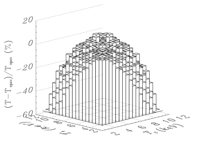
Figure 2: Left panel: reduced $\chi^{2}$ corresponding to the best fit model of a single-temperature thermal model to the simulated spectra of a two-temperature thermal model in the case $Z=0$. Each spectral fit has $\approx 500$ d.o.f. Solid and dashed histograms indicate the fits for which the null hypothesis probability is larger and smaller than 5 per cent, respectively. Right panel: percentile difference between the calculated ($T$) emission-weighted and spectroscopic ($T_{\rm spec}$) temperatures as a function of the temperatures of the lower and higher model components ($T_{1}$ and $T_{2}$, respectively).

3 Spectroscopic Projected Temperature from Chandra  Observations

In the previous section we argued that from a purely analytic point of view the spectrum of a multi-temperature thermal model cannot be reproduced by any single temperature thermal model. In the real world things may be a bit different as, even assuming the most favorable conditions, observed spectra are affected by at least the following factors: i) convolution with the instrument response; ii) Poisson noise; iii) instrumental and cosmic backgrounds. These factors all conjure to distort and, at some level, confuse the observed spectra. Consequently it can happen that, under some circumstances, observed spectra produced by multi-temperature thermal sources may be well fitted by single-temperature thermal models which have little to do with the real temperature, but nevertheless are statistically indistinguishable from it. In the present section we want to address exactly this issue. In order to do that, we generated a number of multi-temperature spectra and performed the standard fitting procedure using a single-temperature model.

To simulate the spectra we used the command fakeit in the utility XSPEC (Arnaud 1996; see, e.g., Xspec User’s Guide version 11.2.x; Dorman & Arnaud 2001 ). This command creates simulated data from the input spectral model by convolving it with the ancillary response files (ARF) and the redistribution matrix files (RMF), which fully define the response of the considered instrument, and by adding the noise appropriate to the specified integration time. To begin with, in the following subsections we will concentrate on observations made with Chandra  in ACIS-S configuration. In particular, all simulated spectra will be obtained by using the ARF and RMF relative to the aim point of the chip ACIS-S3. Later, we will discuss the differences between ACIS-S3 and the ACIS-I Chandra  and MOS and pn XMM-Newton  detectors. In order to make the simulated spectra more similar to the actual observations, we multiply each spectrum by an absorption model (wabs in XSPEC) that accounts for the galactic absorption. In this paragraph we fix the equivalent hydrogen column density of the absorption model to $n_{H}=10^{20}~{}{\rm cm}^{-2}$.

Our main interest is in the possible spectral distortion induced by instrument response, rather than in the spectral uncertainties connected with the data statistics. For this reason we will assume that the observed spectra have no background, and will rescale exposure times so that the total number counts per spectrum is very large ($N\approx 350,000$).

All simulated spectra presented in this section are fitted by an absorbed single-temperature mekal model using the $\chi^{2}$ statistic, and leaving $n_{H}$, $Z$, and $T$ as free parameters. Spectral fits are done in the $0.3-10$ keV energy band. Regardless of the quality of the fit, from now on we will call spectroscopic temperature $T_{\rm spec}$ the best fit temperature value resulting from the above fitting procedure.

Figure 3: As Fig. 1, but for metallicity $Z=1$.

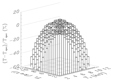
Figure 4: As Fig. 2, but for metallicity $Z=1$.

3.1 Fitting two-temperature thermal spectra with single-temperature models: the zero-metallicity case

We will start by considering the simplest possible model, namely the one in which the gas metallicity is $Z=0$. In this case the source emission is given by the sum of the continuum spectra (see Eq. 5) relative to each plasma component with different temperatures. For didactical purposes we first compare the simulated spectrum of a two-temperature thermal source with the best fit from a single-temperature model. We will assume that the two components of the thermal source have the same emission measure ($k\propto\int n_{e}^{2}dV$). Let us consider three examples, named spectrum 1, 2, and 3 for convenience. All spectra are characterized by the same higher temperature component, fixed at $T_{2}=10$ keV. The lower temperature component is instead $T_{1}=1$ keV, $T_{1}=2.5$ keV, and $T_{1}=5$ keV for spectrum 1, 2, and 3, respectively. In the left, middle, and right panels of Fig. 1 we report the two-temperature thermal input models, the simulated source spectrum, the best fit of the single-temperature thermal model, and the residuals in units of the temperature dispersion $\sigma$ for spectrum 1, 2, and 3, respectively. The figure clearly shows that the source spectrum 1 ($T_{1}=1$ keV) cannot be fitted by a single-temperature thermal model. Conversely, spectrum 3 ($T_{1}=5$ keV) is well fitted by a single temperature thermal model and actually is statistically indistinguishable from it. It is interesting to note that also spectra with low-temperature components $T_{1}<5$ keV can actually be fitted quite reasonably by a single-temperature model: in fact, although spectrum 2 ($T_{1}=2.5$ keV) shows some small departures from its best fit single-temperature model (see the middle panels of Fig. 1), the $\chi^{2}$/d.o.f=526/513 indicates that the fit is still statistically acceptable.

Starting from the three examples above we can explore the intervals of $T_{1}$ and $T_{2}$ required for the source spectra to be well fitted by a single-temperature model. To do so, we produced a large set of two-temperature source spectra with different $T_{1}$ and $T_{2}$, and estimated the spectroscopic temperature for each.

The first interesting result we find is the following: consistently with what found by Mathiesen & Evrard (2001), whenever the lower temperature component is at $T>2$ keV, then almost any two-temperature spectrum can be well fitted by a single-temperature model. This is clearly shown on the left panel of Fig. 2, where we report the reduced $\chi^{2}$ relative to the best fit model of a single-temperature thermal model to the simulated spectra of a two-temperature thermal model. The different line styles indicate if the fit is statistically acceptable or not. In particular, solid and dashed histograms refer to the fits for which the null hypothesis has a probability $>5$ per cent (statistically acceptable fit) or $<5$ per cent (statistically unacceptable fit), respectively. We also notice that the reduced $\chi^{2}$ is always very close to unity, except in few cases where the lower temperature component is at $T\sim 2$ keV and the higher temperature component is at $T>8$ keV. It is important to say that, for lower temperature components at $T<2$ keV, our results show that a single-temperature model is generally not a good fit, unless the difference $|T_{2}-T_{1}|$ is small ($<0.5$ keV). In particular, the lower the temperature of the low-temperature component, the smaller should be difference $|T_{2}-T_{1}|$ in order for its spectrum to be compatible with a single-temperature model.

A second important result we find is that the spectroscopic temperature $T_{\rm spec}$ is always lower than the bolometric emission-weighted temperature, in agreement with reports by some authors (see, e.g., Mathiesen & Evrard 2001; Gardini et al. 2004). This is clearly shown on the right panel of Fig. 2, where we plot the percentile difference between the emission-weighted and spectroscopic temperatures as a function of the lower and higher temperature components of the model: we notice that the larger $|T_{2}-T_{1}|$, the larger this difference, with values as large as 60 per cent for $T_{2}<12$ keV that can be even larger for higher $T_{2}$.

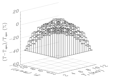
Figure 5: Percentile difference between the calculated ($T$) emission-measure-weighted $T$ (with weight $W\propto n_{e}^{2}$) and the spectroscopic ($T_{\rm spec}$) temperatures as a function of the lower and higher model component temperatures ($T_{1}$ and $T_{2}$, respectively).

3.2 Fitting two-temperature thermal spectra with single-temperature models: the case $Z=1$

We now study the effect of the line emission on the spectroscopic temperature estimates. To do that we repeat the analysis of § 3.2, but now assuming $Z=1$.

As done in the previous subsection, we first show the spectra for the three example models, namely spectra 1, 2, and 3. On the left, middle, and right panels of Fig. 3 we report the two-temperature thermal input models, the simulated source spectrum, the best-fit single-temperature thermal model, and the residuals in terms of $\sigma$ for spectrum 1, 2, and 3, respectively. By comparing Fig. 1 with Fig. 3 we notice that the presence of metals in the plasma induces the formation of lines that may not be reproduced by the best-fit single-temperature model, as clearly shown in the middle panels of Fig. 3. Although the continuum of the source spectrum is very well reproduced by the best fit single-temperature model (see. Fig. 1), the line emission is under-predicted at $1$ keV and over-predicted at $7$ keV (see residual plot in Fig. 3). This suggests that single-temperature models are not suited to fit multi-temperature spectra. Nevertheless, when the low-temperature component is high enough, then a single-temperature model can still fit very well a two-temperature source spectrum, and again it becomes statistically indistinguishable from it (right panels of Fig. 3). This is because the higher the temperatures, the less important the line contribution to the final spectrum; in such cases the source with $Z=1$ becomes more and more similar to that with $Z=0$.

As done in § 3.1, we produced a set of synthetic two-temperature source spectra with different $T_{1}$ and $T_{2}$, and estimated for each the spectroscopic temperature. In the left panel of Fig. 4 we report the reduced $\chi^{2}$ relative to the best fit single-temperature model. As expected, we find that in this case the number of source spectra that cannot be fitted by a single-temperature model is higher. Nevertheless, all source spectra whose lower temperature component is smaller than 3 keV continue to be statistically indistinguishable from a single-temperature model.

Is is worth noticing that also in the case with $Z=1$ we find that the spectroscopic temperature is always lower than the emission weighted one, as clearly shown in the right panel of Fig. 4. We also notice that the observed percentile difference in temperature is higher compared with the case with $Z=0$, although only by a few per cent.

We also tested the goodness-of-fit of a much simpler emission-measure-weighted temperature function, i.e. the one obtained by assuming $\Lambda(T)=1$ (see § 2.1). The percentile difference between the spectroscopic and emission-measure-weighted temperature calculated in this way is shown in Fig. 5. Paradoxically, we find that this simpler temperature definition fares better than the other one, even if it still overpredicts $T_{\rm spec}$ with differences that, for $T_{2}<12$ keV, can be as large as 40 per cent. We must add that a different definition of $T_{\rm ew}$, which uses the cooling function integrated in the telescope energy band ($\Lambda(T)=\int_{E_{\rm min}}^{E_{\rm max}}\epsilon_{E}dE$), gives results in-between the two discussed here. These results demonstrate that none of the emission-weighted temperature functions so far used in the literature actually provides a good approximation of the projected spectroscopic temperature obtained directly from observations.

For completeness, we conclude this section by reporting the effects of projection on the hydrogen column density and metallicity estimates. To do that we compare the fitted $n_{H}$ and $Z$ of the single-temperature model with the input values. Percentile differences are shown in the left and right panels of Fig. 6, respectively. Interestingly, we find that both the measured $n_{H}$ and $Z$ are different from the input values. This difference, however, is always within 10 per cent.

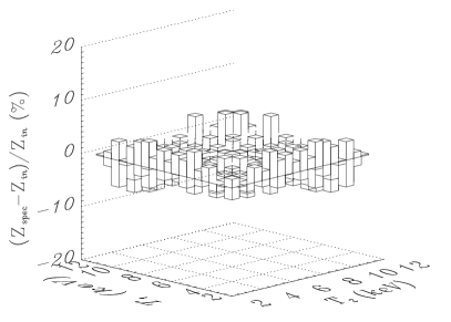
Figure 6: Percentile difference between the value obtained by fitting a single-temperature model to a two-temperature source spectra and the input value. Left and right panels refer to the equivalent hydrogen column density $n_{H}$ (input value $n_{H_{\rm in}}=10^{20}{\rm cm}^{-2}$) and to the metallicity $Z$ in solar units (input value $Z_{\rm in}=1$).

Figure 7: Percentile difference between the calculated ($T$) and the spectroscopic ($T_{\rm spec}$) temperature a a function of the lower and higher model component temperatures ($T_{1}$ and $T_{2}$, respectively). To calculate $T$ we use the spectroscopic-like temperature $T_{\rm sl}$ defined in Eq. 14 with the value of $\alpha$ chosen in order to minimize the value of $\Delta$. Left panel: observational conditions defined as in § 3.1 (to be compared with the right panel of Fig. 2). Right panel: observational conditions defined as in § 3.2 (to be compared with the right panel of Fig. 4).

4 Approximate formula to estimate Chandra  and XMM-Newton  spectroscopic temperatures

In the previous section we have shown that, under some circumstances, a multi-temperature source spectrum can be fitted by a single-temperature model, providing the estimate $T_{\rm spec}$. We have also demonstrated that $T_{\rm spec}$ is always lower than the bolometric emission-weighted temperature $T_{\rm ew}$. In this section we wish to derive a projected emission-weighted temperature formula that can better approximate the spectroscopic one.

The idea is quite simple: given a multi-temperature thermal emission we want to identify the one temperature whose spectrum is closest to the observed spectrum. From now on, we will call $T_{\rm sl}$ this ”spectroscopic-like” temperature. If we assume two thermal components with constant densities $n_{1}$, $n_{2}$, and temperatures $T_{1}$, $T_{2}$, respectively, requiring matching spectra means that

$$\begin{array}[]{l}n_{1}^{2}\zeta(Z,T_{1})\frac{1}{\sqrt{T}_{1}}\exp(-\frac{E}{kT_{1}})+n_{2}^{2}\zeta(Z,T_{2},)\frac{1}{\sqrt{T}_{2}}\exp(-\frac{E}{kT_{2}})\\ \approx A\zeta(Z,T_{\rm sl})\frac{1}{\sqrt{T}_{\rm sl}}\exp(-\frac{E}{kT_{\rm sl}}),\\ \end{array}$$ (7)

where $A$ is an arbitrary normalization constant and $\zeta(Z,T)$ is a parametrization function that accounts for the total Gaunt factor and partly for the line emission.

Both Chandra  and the XMM-Newton  are most sensitive to the soft region of the X-ray spectrum, so we can expand both sides of Eq. 7 in Taylor series, to the first order in $E/kT$:

$$\begin{array}[]{l}n_{1}^{2}\zeta(Z,T_{1})\frac{1}{\sqrt{T}_{1}}(1-\frac{E}{kT_{1}})+n_{2}^{2}\zeta(Z,T_{2})\frac{1}{\sqrt{T}_{2}}(1-\frac{E}{kT_{2}})\\ \approx A\zeta(Z,T_{\rm sl})\frac{1}{\sqrt{T}_{\rm sl}}(1-\frac{E}{kT_{\rm sl}}).\\ \end{array}$$ (8)

By equating the zero-th and first-order terms in $E$, we finally find the equation defining the spectroscopic-like temperature:

$$T_{\rm sl}\approx\frac{n_{1}^{2}\zeta(Z,T_{1})/T_{1}^{1/2}+n_{2}^{2}\zeta(Z,T_{2})/T_{2}^{1/2}}{n_{1}^{2}\zeta(Z,T_{1})/T_{1}^{3/2}+n_{2}^{2}\zeta(Z,T_{2})/T_{2}^{3/2}}.$$ (9)

The extension of Eq. 9 to a continuum distribution of plasma temperatures in a volume $V$ is trivial:

$$T_{\rm sl}\approx\frac{\int n^{2}\zeta(Z,T)/T^{1/2}dV}{\int n^{2}\zeta(Z,T)/T^{3/2}dV}.$$ (10)

To calculate the function $\zeta(Z,T)$ we consider the fact that it gives, together with $n^{2}$, the relative contribution of the spectral component with temperature $T$ to the total spectrum. The amplitude of this normalization contribution is set partly by the total Gaunt factor, partly by the line emission. In principle, their relative importance depends on the details of the instrument/analysis used (e.g. the energy band used for the fit) and on the observational conditions (e.g. low or high galactic absorption regions). However, for temperatures and metallicities realistic in clusters of galaxies ($0<Z<1$, $0.5~{}{\rm keV}<T<20~{}{\rm keV}$) the total Gaunt factor depends essentially on the temperature, and can be approximated by a power-law relation:

$$G_{c}(Z,T,E)\approx(T/{\rm keV})^{\eta},$$ (11)

where $\eta\approx 0.25$ (see, e.g., Mewe & Gronenschild 1981). The effect of the lines is to increase the plasma emissivity, especially at low energies: this effect can also be approximated by a power-law of the temperature. Thus in the following we will assume for $\zeta(Z,T)$ the following functional form:

$$\zeta(Z,T)\propto(T/{\rm keV})^{\alpha},\\$$ (12)

where the parameter $\alpha$ depends on the specific observational conditions and on the used instrument, so it needs to be appropriately calibrated. We do this by adopting the following procedure: we select some specific observation conditions, simulate a set of two-temperature source spectra as explained in § 3 and calculate the mean value of the percentile variation of $T_{\rm sl}$ with respect to $T_{\rm spec}$:

$$\Delta=\frac{1}{N}\sum_{T_{1},T_{2}}\sqrt{\Big{(}\frac{T_{\rm sl}-T_{\rm spec}}{T_{\rm spec}}\Big{)}^{2}}.$$ (13)

In the previous formula the sum is extended to all the $N$ simulated source spectra with $3~{}{\rm keV}<T_{1}<20~{}{\rm keV}$ and $3~{}{\rm keV}<T_{2}<20~{}{\rm keV}$. The variable $\alpha$ is obtained though a minimization procedure of $\Delta$.

Table 1: Value of $\alpha$ and corresponding minimum $\Delta$ for different observational conditions

Number	Detector	$n_{H}$	$Z$	$E_{\rm min}$	$\alpha$	minimum $\Delta$
		($10^{22}$cm-2)		(keV)
1	ACIS-S3	0	0	0.3	0.73	2.1
2	ACIS-S3	1	0	0.3	0.86	3.7
3	ACIS-S3	0	1	0.3	0.41	1.4
4	ACIS-S3	1	1	0.3	0.63	2.3
5	ACIS-S3	0	0	1.0	0.79	3.0
6	ACIS-S3	1	0	1.0	0.89	3.9
7	ACIS-S3	0	1	1.0	0.48	2.1
8	ACIS-S3	1	1	1.0	0.82	2.5
1	MOS	0	0	0.3	0.82	2.3
2	MOS	1	0	0.3	0.92	3.7
3	MOS	0	1	0.3	0.46	1.5
4	MOS	1	1	0.3	0.81	2.3
5	MOS	0	0	1.0	0.86	3.4
6	MOS	1	0	1.0	0.91	4.0
7	MOS	0	1	1.0	0.55	2.2
8	MOS	1	1	1.0	0.96	2.4

To show how well $T_{\rm sl}$ reproduces the actual $T_{\rm spec}$, we apply it to the cases discussed earlier in § 3.1 and § 3.2. The minimization procedure of $\Delta$ returns $\alpha=0.86$ and $\alpha=0.65$ for the Z=0 and Z=1, respectively. The resulting percentile variation between $T_{\rm sl}$ and $T_{\rm spec}$ for these two cases is shown in Fig. 7, on the left and right panels, respectively. The figure clearly shows that, unlike $T_{\rm ew}$, $T_{\rm sl}$ provides a good estimate of the observed spectroscopic temperature, at a level better than 2-3 per cent.

We now study how the power index $\alpha$ depends on the observational conditions for all the Chandra  and XMM-Newton  detectors, and how it changes as a function of the minimum energy $E_{\rm min}$ considered in the spectral fitting. In Table 1 we report for some of the cases considered the value of $\alpha$ obtained using the minimization procedure, and the corresponding value of minimum $\Delta$. The cases reported in the table are only a few examples of those we actually considered. They represent extreme situations for galaxy clusters, in the sense that we explicitly considered strong and null galactic absorption ($n_{H}=10^{22}~{}{\rm cm}^{-2}$ and $n_{H}=0~{}{\rm cm}^{-2}$, respectively), and solar (Z=1) and zero (Z=0) metal abundances. The values of $\alpha$ and the corresponding minimum $\Delta$ from Table 1 are also shown in Fig. 8. Open circles and filled triangles refer to Chandra  ACIS-S3 and XMM-Newton  MOS, respectively. From Fig. 8 it is clear that, as expected, the value of $\alpha$ minimizing the discrepancy between $T_{\rm sl}$ and $T_{\rm spec}$ depends on the actual observation conditions. Nevertheless, we notice that: i) $\alpha$ and $\Delta$ are very close to each other for Chandra  and XMM-Newton; ii) the minimum $\Delta$ is generally very low and smaller than 4 per cent. Following these considerations we explored the interval in $\alpha$ for which the corresponding value of $\Delta$ is smaller than 5 per cent. The results are reported in Fig. 8, where this range is shown as y-axis error bars. We notice that all the error bars overlap. This is important as it means that, regardless of the observational conditions, we can select a value of $\alpha$ (which we call $\alpha_{u}$) so that $T_{\rm sl}$ can reproduce $T_{\rm spec}$ with an accuracy better than $5$ per cent on average. As shown by the solid horizontal line in Fig. 8 a good choice for Chandra  and XMM-Newton  is $\alpha_{u}=0.75$.

Figure 8: Value of $\alpha$ and corresponding minimum value of $\Delta$ for the observational conditions reported in Table 1. Open circles and filled triangles refer to Chandra  ACIS-S3 and XMM-Newton  MOS, respectively. The error bars show the range in $\alpha$ where $\Delta<5$ per cent (see text). The horizontal line indicates $\alpha=0.75$.

Figure 9: Percentile difference between the calculated ($T$) and the spectroscopic ($T_{\rm spec}$) temperatures as a function of the lower and higher model component temperatures ($T_{1}$ and $T_{2}$, respectively). To calculate $T$ we use the spectroscopic-like temperature $T_{\rm sl}$ defined in Eq. 14 assuming $\alpha=\alpha_{u}\equiv 0.75$. The panels from up to down, left to right, correspond to the observational conditions 1 to 4, reported in Table 1 with ACIS-S3, respectively.

The accuracy of $T_{\rm sl}$ when we adopt $\alpha_{u}=0.75$ is shown in Fig. 9 and Fig. 10, where we report the percentile variation between the values of $T_{\rm sl}$ and $T_{\rm spec}$ obtained in different observational conditions with the Chandra  ACIS-S3 detector. In Fig. 9 and Fig. 10 the values of $T_{\rm spec}$ were obtained by fitting the spectra down to $E_{\rm min}=0.3$ keV and $E_{\rm min}=1$ keV, respectively. The four panels in each figure correspond to ($n_{H}=0\times 10^{22}$cm^-2, $Z=0$), ($n_{H}=1\times 10^{22}$cm^-2, $Z=0$), ($n_{H}=0\times 10^{22}$cm^-2, $Z=1$), and ($n_{H}=1\times 10^{22}$cm^-2, $Z=1$). As expected, for most of the temperature combinations of the source spectra, $T_{\rm sl}(\alpha_{u}=0.75)$ gives a good estimate of $T_{\rm spec}$ at a level better than 5 per cent, while the difference is higher only for a few spectra (see, e.g., upper-right and lower-left panels of Fig. 9 and Fig. 10). However, the only spectra for which the discrepancy is higher than $5$ per cent are those on the border of the temperature plane, i.e. those whose the lower temperature component in the source model is $T=3$ keV. As already explained in § 3.1 and § 3.2, this temperature represents a sort of “borderline” value for Chandra  and XMM-Newton. Thus, the reason of such higher discrepancy is simply explained by the inability to properly define a spectroscopic projected temperature for these spectra, due to the poor quality of the fit with a single temperature model (see left panels of Fig. 2 and 4).

Figure 10: As Fig. 9, but the panels from up to down, left to right, correspond now to the observational conditions 5 to 8 reported in Table 1 with ACIS-S3, respectively.

To summarize the results of this section, we claim that the spectroscopic-like temperature defined by:

$$T_{\rm sl}(\alpha)\approx\frac{\int n^{2}T^{\alpha}/T^{1/2}dV}{\int n^{2}T^{\alpha}/T^{3/2}dV},$$ (14)

with $\alpha=\alpha_{u}=0.75$, gives a good approximation of the spectroscopic temperature $T_{\rm spec}$ obtained from data analysis of Chandra  and XMM-Newton  observations.

We notice that Eq. 14 can be rewritten in the general form of Eq. 1:

$$\begin{array}[]{rl}T_{\rm sl}&=\frac{\int WTdV}{\int WdV},\\ W&=\frac{n^{2}}{T^{3/4}}.\\ \end{array}$$ (15)

It is interesting to note that $T_{\rm sl}$ weights each thermal component directly by the emission measure but, unlike $T_{\rm ew}$, inversely by their temperature to the power of $3/4$. This means that, beside being biased toward the densest regions of the clusters, the observed spectroscopic temperature is also biased toward the coolest regions. In the next sections we will discuss some important implications of this bias.

5 Testing Spectroscopic-Like Temperature on Hydro-N-body simulation

Using a simplified two-temperature thermal model we have shown that the spectroscopic-like temperature $T_{\rm sl}$ provides a good approximation to the spectroscopically derived temperature $T_{\rm spec}$. Here we wish to extend this study by showing the goodness of $T_{\rm sl}$  in reproducing $T_{\rm spec}$  in a more general case.

In order to do that, we follow the same procedure used in Gardini et al. (2004), where we use the output of an hydro-N-body simulation and the X-ray MAp Simulator (X-MAS) to compare $T_{\rm spec}$ with $T_{\rm ew}$ for a simulated cluster of galaxies. Here we use the same simulation to extend the comparison to $T_{\rm sl}$.

Let us briefly remind that the cluster simulation used in Gardini et al. (2004) was selected from a sample of 17 objects obtained by re-simulating at higher resolution a patch of a pre-existing cosmological simulation. The assumed cosmological framework is a cold dark matter model in a flat universe, with present matter density parameter $\Omega_{m}=0.3$ and a contribution to the density due to the cosmological constant $\Omega_{\Lambda}=0.7$; the baryon content was set to $\Omega_{B}=0.03$; the value of the Hubble constant (in units of 100 km/s/Mpc) is $h=0.7$, and the power spectrum normalization is given by $\sigma_{8}=0.9$. The re-simulation method we used, called ZIC (for Zoomed Initial Conditions), is described in detail in Tormen et al. (1997), while an extended discussion of the properties of the whole sample of these simulated clusters is presented elsewhere (Tormen et al. 2004; Rasia et al. 2004). Here we remind only some of the characteristics of the cluster used in this paper. The simulation was obtained by using the publicly available code GADGET (Springel et al. 2001); during the run, starting at redshift $z_{\rm in}=35$, we took 51 snapshots equally spaced in $\log(1+z)$, from $z=10$ to $z=0$. The cluster virial mass at $z=0$ is $1.46\times 10^{15}h^{-1}M_{\odot}$, corresponding to a virial radius of $2.3h^{-1}$ Mpc; the mass resolution is $4.5\times 10^{9}h^{-1}M_{\odot}$ per dark particles and $5\times 10^{8}h^{-1}M_{\odot}$ per gas particles; the total number of particles found inside the virial radius is 566,374, 48 per cent of which are gas particles. The gravitational softening is given by a $5h^{-1}$ kpc cubic spline smoothing.

In the left panel of Fig. 11 we report the emission-weighted temperature map of the simulated clusters overlaid to the cluster flux distribution from Gardini et al. (2004). The figure clearly shows that the cluster is far from isothermal. Among other features, we point to the reader the presence in this map of two shock fronts. The first is in the lower-left corner, and is produced by the motion toward the cluster centre of the innermost of the two subclumps present in that region. This front has a post-shock gas temperature of approximately $18$ keV. A similar, but weaker, shock front is located in front of the subclump, at the centre of the Eastern side of the cluster. For comparison, on the right panel of Fig. 11 we report the spectroscopic-like temperature map of the same cluster, overlaid to the cluster flux distribution. An immediate thing to notice is that the map of $T_{\rm sl}$ appears cooler than the map of $T_{\rm ew}$. This is consistent with the fact that, unlike $T_{\rm ew}$, $T_{\rm sl}$ is biased toward the lowest values of the dominant temperature components along the line of sight. Another very important point is that both shock fronts, which are clearly evident in the emission-weighted temperature map, are no longer detected in the $T_{\rm sl}$ map. This aspect will be further discussed in § 6 below.

In the following subsections we will compare $T_{\rm spec}$, $T_{\rm ew}$ and $T_{\rm sl}$ in two cases of practical interest: the determinations of the projected cluster temperature map and the determination of the radial profile. To do that we will use the 300 ks Chandra  ACIS-S3 X-MAS “observation” of this cluster from Gardini et al. (2004). As explained in that paper, the observation for this particular cluster was performed by fixing the cluster metallicity to $Z=0.3\,Z_{\odot}$ and the column density to $N_{H}=5\times 10^{20}$ cm^-2; data were analysed by applying the standard procedures and tools used for real observations. We refer to Gardini et al. (2004) for more details on the data analysis. Here we just remind that $T_{\rm spec}$ is obtained by fitting the spectra in the [0.6,9.0] keV energy band with a single/temperature absorbed mekal model, after fixing the cluster redshift, metallicity, and hydrogen column density to the values used as inputs to compute the Chandra  observation.

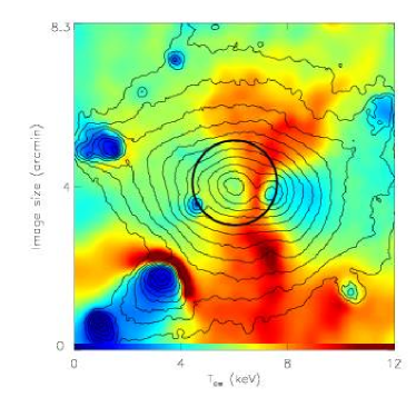
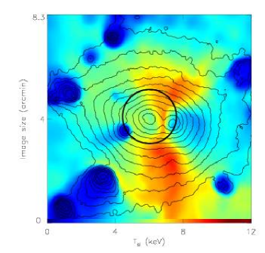
Figure 11: Comparison of the map of the emission-weighted temperature $T_{\rm ew}$  (left-panel) and the spectroscopic-like temperature $T_{\rm sl}$  (right-panel) for the simulated cluster of galaxy. Both maps are obtained by using the gas particles of the hydro-N-body simulation and are binned in $1\arcsec$ pixels. The contour levels correspond to the cluster flux distribution. The circle shows the cluster region from which the temperature profile sispayed in Fig. 15 has been extracted.

5.1 Cluster projected temperature map

As mentioned above, we used the spectroscopic temperature map published in Gardini et al. (2004). That map was obtained by subdividing the cluster image in squares large enough to contain at least 250 net photons. The projected spectroscopic temperature map $T_{\rm spec}$ is shown in Fig. 12. In order to make a direct comparison of this map to those with emission-weighted and the spectroscopic-like temperatures, we decreased the resolution of the latter to match the resolution of the former.

In the left panel of Fig. 13 we report the same map of $T_{\rm ew}$ shown on the left panel of Fig. 11, but re-binned as the map of Fig. 12.

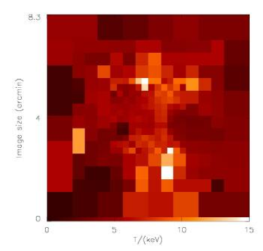
Figure 12: Spectroscopic temperature map of the simulated cluster of galaxy as derived from the spectroscopic analysis of the Chandra  “observation” with the package X-MAS (from Gardini et al. 2004).

To highlight the temperature differences between the spectroscopic and the emission-weighted temperature maps, in the right panel of Fig. 13 we show the percentile difference of $(T_{\rm ew}-T_{\rm spec})/T_{\rm spec}$. For better visualization we only show the pixels where this difference is significant to at least $3\sigma$ confidence level, i.e. $|(T_{\rm ew}-T_{\rm spec})/\sigma_{\rm spec}|>3$, being $\sigma_{\rm spec}$ the 68 per cent confidence level error associated with the spectroscopic temperature measurement. This plot clearly shows that there are many regions where the difference between $T_{\rm ew}$ and $T_{\rm spec}$ is significant to better than $\ga 3\sigma$ confidence level. Furthermore, for these pixels the discrepancy ranges from 50 per cent to 200 per cent and even more. Of particular relevance are two cluster regions showing a shock front in the emission-weighted map, in the left panel of Fig. 11. The map of the percentile difference between $T_{\rm ew}$  and $T_{\rm spec}$  shows discrepancies of 100-200 per cent, indicating that shock fronts predicted in the emission weighted map are no longer detected in the observed spectroscopic map.

Conversely, in the left panel of Fig. 14 we show the same map of $T_{\rm sl}$ shown in the right panel of Fig. 11, but re-binned as the spectroscopic temperature map of Fig. 12. As we did for the emission-weighted temperature map, in the right panel of Fig. 14 we show the percentile difference of $(T_{\rm sl}-T_{\rm spec})/T_{\rm spec}$. Again we only visualize the pixels for which the difference is significant to at least $3\sigma$ confidence level. The presence in this map of fewer pixels clearly indicates that the match between $T_{\rm sl}$ and $T_{\rm spec}$  is much better than the one between $T_{\rm spec}$  and $T_{\rm ew}$. Furthermore, most of these pixels shows very small temperature discrepancies, being smaller than $10$ per cent. Only in 6 pixels we find a slightly higher temperature discrepancy, but in any case smaller than $20$ per cent.

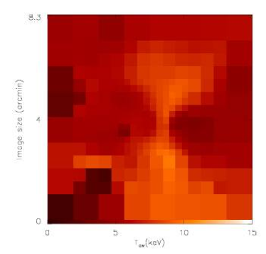
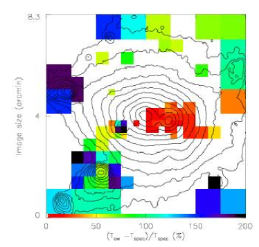
Figure 13: Left panel: emission-weighted temperature map of the simulated cluster of galaxies shown in the left panel of Fig. 11 re-binned to match the spatial resolution of the spectroscopic temperature map shown in Fig. 12. Right panel: percentile difference between the spectroscopic and emission-weighted temperature maps. In this map we show only the regions where the significance level of the temperature discrepancy is at least $3\sigma$, i.e. $|(T_{\rm ew}-T_{\rm spec})/\sigma_{\rm spec}|>3$, where $\sigma_{\rm spec}$ is the 68 per cent confidence level error associated to $T_{\rm spec}$.

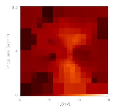
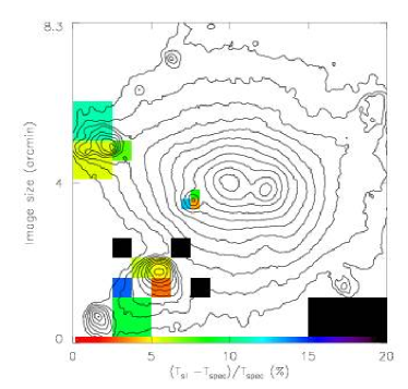
Figure 14: Left panel: spectroscopic-like temperature map for the simulated cluster of galaxies shown in the right panel of Fig. 11 re-binned to match the spatial resolution of the spectroscopic temperature map shown in Fig. 12. Right panel: percentile difference between the spectroscopic and the spectroscopic-like temperature maps. In this map we show only the regions where the significance level of the temperature discrepancy is at least $3\sigma$, i.e. $|(T_{\rm sl}-T_{\rm spec})/\sigma_{\rm spec}|>3$, where $\sigma_{\rm spec}$ is the 68 per cent confidence level error associated to $T_{\rm spec}$.

This demonstrates that the spectroscopic-like temperature gives a much better estimate of the observed spectroscopic temperature than the widely used emission-weighted one. It is worth noting that in the previous map 3 out of 6 pixels where the discrepancy is between 10 and 20 per cent correspond to cluster regions with very low surface brightness. We believe that the observed discrepancy in this case is simply related to the very poor statistics used to determine $T_{\rm spec}$. In the other 3 cases the relatively higher discrepancy is instead related to the fact that the thermal components of these regions that contribute to the spectra have a quite large spread of temperatures and, because the lower (dominant) thermal component is at $T<3$ keV, $T_{\rm spec}$  cannot be unequivocally identified: a proper spectral analysis would require a fit with a two-temperature model.

It is very important to say that, unlike the emission-weighted, the map on the right panel of Fig. 14 does not show big discrepancies between $T_{\rm sl}$  and $T_{\rm spec}$  in both shock cluster regions. This clearly indicate that $T_{\rm sl}$  does a much better job than $T_{\rm ew}$  in predicting the projected spectral properties of such peculiar thermal features.

5.2 Cluster projected temperature profile

To conclude this section we also tested the accuracy of $T_{\rm sl}$  in predicting the observed spectroscopic temperature profile. We again used the spectroscopic projected temperature profile of Gardini et al. (2004). This was obtained by extracting spectra from circular annuli centred on the cluster centre, out to the radius identified by the circle in Fig. 11. The size of the bin was chosen in order to have approximately the same number of photons inside each annulus. The spectroscopic temperature profiles $T_{\rm spec}$, together with their relative 68 per cent confidence level errors $\sigma_{\rm spec}$, are shown as filled circles in Fig. 15. In the same figure we show the emission-weighted temperature and the spectroscopic-like temperature. As already discussed in Gardini et al. (2004), we notice that the emission-weighted temperature $T_{\rm ew}$ profile does not reproduce the spectroscopic temperature profiles $T_{\rm spec}$. In particular we confirm that the spectral temperatures are systematically lower than the emission-weighted ones. Conversely, the spectroscopic-like temperature profile provides a much more accurate estimate, and falls within the error bars of the “observed” spectroscopic temperature profile everywhere but in two annuli.

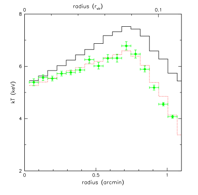
Figure 15: Temperature profiles of the simulated cluster of galaxies. Filled circles refer to the mean spectroscopic temperature profile from Gardini et al. (2004) and correspond to the region shown as a circle in Fig. 11; error bars are at $68$ per cent confidence level for one interesting parameter. Solid and dotted histograms refer to the mean emission-weighted and spectroscopic-like temperature profiles directly extracted from the simulation.

6 Discussion and Conclusions

In this paper we have studied the problem of performing a proper comparison between temperatures obtained from the data analysis of X-ray observations (i.e. projected spectroscopic temperatures, $T_{\rm spec}$) and temperatures derived directly from hydro-N-body simulations (projected emission-weighted temperatures $T_{\rm ew}$). In § 2.2 we show analytically that $T_{\rm spec}$  is not a well defined quantity. In fact, it results from the fit of a single-temperature thermal model to a multi-temperature source spectrum; however, since the former cannot accurately reproduce the spectral properties of the latter, it follows that $T_{\rm spec}$  cannot be unequivocally identified. Generally speaking, this means that a reliable comparison between simulations and observations can only be done through the actual simulation of the spectral properties of the simulated clusters: these properties will then be directly compared with the observed ones. Nevertheless, observed spectra are affected by a number of factors that distort and confuse some of their properties. In some circumstances multi-temperature thermal source spectra may appear statistically indistinguishable from a single-temperature model. In § 3 we study this aspect focusing our attention on observations of clusters of galaxies made using the CCD detectors of Chandra  and XMM-Newton. These detectors are characterized by having both a similar intermediate energy resolution and a similar energy response. From our study we find two very important results that for convenience we summarize below.

1. Given a multi-temperature source spectrum, if the lowest dominant temperature component has $T_{1}>2-3$ keV, then a fit made with a single-temperature thermal model is statistically acceptable regardless of the actual spread in temperature distribution.

   On the other hand, multi-temperature sources with $T_{1}<2$ keV will most likely require multi-temperature spectral models. This is equivalent to say that $T_{\rm spec}$  can be properly defined only for spectra with $T_{1}>2-3$ keV. For lower temperatures the identification of multi-temperature observed spectra with a single temperature is not appropriate. It is important to say that this result is intrinsically related to the characteristics of the X-ray detector used for the observation (e.g. its energy pass band and resolution) and not to a possible inadequate photon statistics. In fact our result was obtained in the limit of high spectral photon number (see § 3). It is self-evident that this conclusion will be true also for all the detectors whose spectral properties are similar or worse than those on board of Chandra  and XMM-Newton, while this will not be true for X-ray spectrographs with either a much larger energy pass band or a much higher energy resolution.

2. The emission-weighted temperature $T_{\rm ew}$, originally introduced to provide a better comparison between simulations and observations, in practice does not properly estimate the spectroscopic temperature $T_{\rm spec}$. In particular $T_{\rm ew}$  tends to overestimate $T_{\rm spec}$. This mismatch depends on the thermal inhomogeneity of the observed multi-temperature source: the larger the spread in temperature of the dominant components in the observed spectrum, the larger the discrepancy. In § 4 we derive a new formula, the spectroscopic-like temperature function $T_{\rm sl}$ (see Eq. 15), and show that $T_{\rm sl}$  can approximate $T_{\rm spec}$  to a level better than 10 per cent regardless of the temperature spread. It is worth noticing that $T_{\rm sl}$  weights each thermal component directly by the emission measure but inversely by their temperature to the power of $3/4$. This explains why the observed $T_{\rm spec}$  is biased toward the lower values of the dominant thermal components.

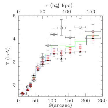
Figure 16: Temperature profiles of the galaxy cluster 2A 0335 (from Mazzotta et al. 2003). Filled triangles and open circles refer to the projected cluster temperature profile in the northern and southern sectors, respectively. Open squares indicate the overall projected cluster temperature profile obtained from a circular radial analysis. The upper and the lower histograms show the profiles for the emission-weighted and spectroscopic-like temperatures, respectively. These histograms have been obtained by combining the northern and southern temperature profiles.

These two results have important observational and theoretical implications for the study of X-ray clusters of galaxies. First of all the equivalence between observed “hot” multi-temperature spectra and single-temperature models implies that, using the CCD detectors of Chandra  and XMM-Newton, it is observationally impossible to disentangle the single or multi-temperature nature of any observed spectrum whose projected temperature is higher than $3$ keV by performing a simple overall X-ray spectral analysis. In addition, the temperature derived from this spectral analysis is not the emission-weighted value, but it is biased toward the lowest dominant thermal component of the overall spectrum. The consequences for studies of temperature profiles in clusters are immediate. In virtually all works on the subject, in fact, the cluster temperature profile is derived by extracting spectra from concentric circular or elliptical annuli centred on the cluster X-ray peak. Together with the cluster gas distribution, this temperature profile is used to estimate the cluster mass by assuming hydrostatic equilibrium. It is self-evident that, if the cluster gas temperature distribution is azimuthally asymmetric, the temperature profile derived from the radial analysis is biased toward lower temperature values and so does the estimated mass. To better show this aspect we discuss the results of the data analysis of the cluster of galaxies 2A 0335+096  selected, as example, among the many published in the literature. In particular, all the temperature measurements discussed below are taken from Mazzotta et al. (2003). In Fig. 16 we compare the projected temperature profiles of the cluster of galaxies 2A 0335+096  extracted from different sectors. Filled triangles and open circles indicate the temperature profiles obtained from the Northern (from -90${}^{\circ}\!$  to 90${}^{\circ}\!$; angles are measured from North toward East) and Southern (from 90${}^{\circ}\!$  to 270${}^{\circ}\!$) sectors of the clusters. As highlighted by Mazzotta et al. (2003), the temperature profile of 2A 0335+096  is clearly azimuthally asymmetric. We notice that in the 100-200 arcsec radial interval the temperature profile of the southern sector is between 30 and 50 per cent hotter than the Northern one. The open squares in Fig. 16 indicate the cluster temperature profile obtained from the circular radial analysis. For convenience we report as histogram the expected temperature profile obtained by combining the Northern and Southern temperature profiles using the emission-weighted formula. From this figure it is evident that, consistently with what discussed so far, the circular radial temperature profile is significantly lower that the expected emission-weighted profile and is biased toward the values of the Northern profile. For completeness in the same figure we added as histogram the temperature profile obtained by combining the Northern and Southern temperature measurements using the spectroscopic-like formula. This latter profile is perfectly consistent with the measured one proving once more that, unlike the emission-weighted temperature, our spectroscopic-like formula provides a very good approximation to the spectroscopic temperature measurements.

It is important to say that, by construction, the difference between $T_{\rm ew}$  and $T_{\rm sl}$  mainly depends on the complexity of the projected thermal structure of the cluster gas. It is clear that the findings of this study are especially relevant for major-merger clusters rather than for relaxed clusters. They may have also important implications for the study of all structures with very strong temperature gradients like, for example, the shock fronts. In fact, because of the temperature bias of $T_{\rm spec}$, shock fronts in real observations appear much weaker than the predictions of virtually all the emission-weighted temperature map published in literature. This has been shown in § 5.1 and is evident in Fig. 11. From this figure we immediately see that the two shock fronts clearly visible in the emission-weighted map are no longer detected in the spectroscopic-like temperature map. This temperature bias may explain why, although simulations predict that shock fronts are quite common in clusters of galaxies, to date we have very few observations of clusters in which they are clearly present.

To conclude we stress once more that the emission-weighted temperature function may give a misleading view of the actual gas temperature structure as obtained from X-ray observations. Thus, since the emission-weighted temperature has no physical meaning (unlike the mass-weighted one), here we propose to theoreticians and N-body simulators to finally discard its use. We remind that great attention must be paid when comparing simulations and X-ray observations. Under the most generic conditions such comparison can only be done through the actual simulation of the spectral properties of the simulated clusters, so that software packages like X-MAS (Gardini et al., 2004) become fundamental. Nevertheless, if the cluster temperature is sufficiently high and if the spectral properties of the detector used for the observation are similar or worse that the ones of Chandra  and XMM-Newton  we showed that our proposed spectroscopic-like temperature function may be considered an appropriate tool for the job.

References

- Arnaud (1996) Arnaud K. A., 1996, in ASP Conf. Ser. 101: Astronomical Data Analysis Software and Systems V XSPEC: The First Ten Years. pp 17–+
- Bartelmann & Steinmetz (1996) Bartelmann M., Steinmetz M., 1996, \mnras, 283, 431
- Blanton et al. (2001) Blanton E. L., Sarazin C. L., McNamara B. R., Wise M. W., 2001, \apjl, 558, L15
- Borgani et al. (2004) Borgani S., Murante G., Springel V., Diaferio A., Dolag K., Moscardini L., Tormen G., Tornatore L., Tozzi P., 2004, \mnras, 348, 1078
- Bryan & Norman (1998) Bryan G. L., Norman M. L., 1998, \apj, 495, 80
- Dorman & Arnaud (2001) Dorman B., Arnaud K. A., 2001, in ASP Conf. Ser. 238: Astronomical Data Analysis Software and Systems X Redesign and Reimplementation of XSPEC. pp 415–+
- Eke et al. (1998) Eke V. R., Navarro J. F., Frenk C. S., 1998, \apj, 503, 569
- Evrard et al. (1996) Evrard A. E., Metzler C. A., Navarro J. F., 1996, \apj, 469, 494
- Fabian et al. (2001) Fabian A. C., Sanders J. S., Ettori S., Taylor G. B., Allen S. W., Crawford C. S., Iwasawa K., Johnstone R. M., 2001, \mnras, 321, L33
- Fabian et al. (2000) Fabian A. C., Sanders J. S., Ettori S., Taylor G. B., Allen S. W., Crawford C. S., Iwasawa K., Johnstone R. M., Ogle P. M., 2000, \mnras, 318, L65
- Frenk & et al. (1999) Frenk C. S., et al. 1999, \apj, 525, 554
- Gardini et al. (2004) Gardini A., Rasia E., Mazzotta P., Tormen G., De Grandi S., Moscardini L., 2004, \mnras, in press, astro-ph/0310844
- Heinz et al. (2002) Heinz S., Choi Y., Reynolds C. S., Begelman M. C., 2002, \apjl, 569, L79
- Johnstone et al. (2002) Johnstone R. M., Allen S. W., Fabian A. C., Sanders J. S., 2002, \mnras, 336, 299
- Kaiser (1986) Kaiser N., 1986, \mnras, 222, 323
- Kang et al. (1994) Kang H., Cen R., Ostriker J. P., Ryu D., 1994, \apj, 428, 1
- Markevitch & et al. (2000) Markevitch M., et al. 2000, \apj, 541, 542
- Markevitch et al. (2001) Markevitch M., Vikhlinin A., Mazzotta P., 2001, \apjl, 562, L153
- Mathiesen et al. (1999) Mathiesen B., Evrard A. E., Mohr J. J., 1999, \apjl, 520, L21
- Mathiesen & Evrard (2001) Mathiesen B. F., Evrard A. E., 2001, \apj, 546, 100
- Mazzotta et al. (2003) Mazzotta P., Edge A. C., Markevitch M., 2003, \apj, 596, 190
- Mazzotta et al. (2002) Mazzotta P., Fusco-Femiano R., Vikhlinin A., 2002, \apjl, 569, L31
- Mazzotta et al. (2002) Mazzotta P., Kaastra J. S., Paerels F. B., Ferrigno C., Colafrancesco S., Mewe R., Forman W. R., 2002, \apjl, 567, L37
- Mazzotta et al. (2001) Mazzotta P., Markevitch M., Vikhlinin A., Forman W. R., David L. P., VanSpeybroeck L., 2001, \apj, 555, 205
- McNamara et al. (2000) McNamara B. R., Wise M., Nulsen P. E. J., David L. P., Sarazin C. L., Bautz M., Markevitch M., Vikhlinin A., Forman W. R., Jones C., Harris D. E., 2000, \apjl, 534, L135
- McNamara et al. (2001) McNamara B. R., Wise M. W., Nulsen P. E. J., David L. P., Carilli C. L., Sarazin C. L., O’Dea C. P., Houck J., Donahue M., Baum S., Voit M., O’Connell R. W., Koekemoer A., 2001, \apjl, 562, L149
- Mewe & Gronenschild (1981) Mewe R., Gronenschild E. H. B. M., 1981, \aaps, 45, 11
- Muanwong et al. (2001) Muanwong O., Thomas P. A., Kay S. T., Pearce F. R., Couchman H. M. P., 2001, \apjl, 552, L27
- Navarro et al. (1995) Navarro J. F., Frenk C. S., White S. D. M., 1995, \mnras, 275, 720
- Rasia et al. (2004) Rasia E., Tormen G., Moscardini L., 2004, \mnras, in press, astro-ph/0309405
- Sanders & Fabian (2002) Sanders J. S., Fabian A. C., 2002, \mnras, 331, 273
- Smith et al. (2002) Smith D. A., Wilson A. S., Arnaud K. A., Terashima Y., Young A. J., 2002, \apj, 565, 195
- Springel et al. (2001) Springel V., Yoshida N., White S. D. M., 2001, New Astronomy, 6, 79
- Sunyaev & Zeldovich (1972) Sunyaev R. A., Zeldovich Y. B., 1972, Comments on Astrophysics and Space Physics, 4, 173
- Thomas et al. (1998) Thomas P. A., Colberg J. M., Couchman H. M. P., Efstathiou G. P., Frenk C. S., Jenkins A. R., Nelson A. H., Hutchings R. M., Peacock J. A., Pearce F. R., White S. D. M., 1998, \mnras, 296, 1061
- Tormen et al. (1997) Tormen G., Bouchet F. R., White S. D. M., 1997, \mnras, 286, 865
- Tormen et al. (2004) Tormen G., Moscardini L., Yoshida N., 2004, \mnras, in press, astro-ph/0304375
- Vikhlinin et al. (2001) Vikhlinin A., Markevitch M., Murray S. S., 2001, \apj, 551, 160
- Young et al. (2002) Young A. J., Wilson A. S., Mundell C. G., 2002, \apj, 579, 560