Reconstructing large running-index inflaton potentials

Abstract

Recent fits of cosmological parameters by the first year Wilkinson Microwave Anisotropy Probe (WMAP) measurement seem to favor a primordial scalar spectrum with a large varying index from blue to red. We use the inflationary flow equations to reconstruct large running-index inflaton potentials and comment on current status on the inflationary flow. We find previous negligence of higher order slow rolling contributions when using the flow equations would lead to unprecise results.
PACS number(s): 98.80.Cq, 11.10.Kk

In the past decade, inflation theory has successfully passed several nontrivial tests. In particular, the recently released Wilkinson Microwave Anisotropy Probe (WMAP) data kogut have detected a large-angle anti-correlation in the temperature–polarization cross-power spectrum, which is the signature of adiabatic superhorizon fluctuations at the time of decouplingWMAP2 . The high-precision WMAP data have been used to fit the cosmological parameters and confront the predictions of inflationary scenarios respectively in Refs. WMAP, and WMAP2, . It is noted that there might be possible discrepancies between predictions and observations on the largest and smallest scales. Basing on this fact Spergel WMAP et al introduced a new parameter: $dn_{s}/d\ln k$ in the fit. With the global fit to WMAPext, 2df 2df and Lyman-$\alpha$ forests forest the authors found a preference of nonzero running at around $2\sigma$. Although the use of Lyman-$\alpha$ data was questioned by Seljak , the fit to WMAP alone favored the running to about $1.5\sigma$: at the pivot scale $k_{0}=0.002~{}{\rm Mpc}^{-1}$, the best-fit values of the scalar power spectrum for WMAP alone being $n_{s}=1.20^{+0.12}_{-0.11}$ and $dn_{s}/d\ln k=-0.077^{+0.050}_{-0.052}$ WMAP2 . It is recently found that the inclusion of VSA data can lead to a negative running at a level of more than $95\%$ confidence when fitting to CMB onlyVSA . Theoretically there have been studies in the literature since the release of the WMAP data on models of inflation which provide a running index required by the WMAP feng ; running . On the other hand, Bridle et al claimed that the need of running should come from the low CMB quadrupole aloneLewis and thereafter many theoretical models were put forwardsmalll . Meanwhile Mukherjee and Wang Wang used the model independent reconstruction of primordial spectrum and found that a running index from blue to red was indeed favored.

The need of large running has been studied widelyWang ; Lewis ; Seljak ; fitWMAP ; Kinney03 after the release of first year WMAP data. At least WMAP could not rule out significant running and if further stands, it could severely constrain inflation model buildings. In the present paper we will use the inflationary flow equations to generate potentials which can lead to large variations in the spectral index.

The inflationary flow equations were firstly introduced by Hoffman and TurnerHT01 to study generic predictions of slow-rolling inflation and for the first time compared with observations in Ref.kunz, . Latter KinneyKinney02 developed the equations as the inflaton potential “generator”, which has been used widely in the literatureWMAP2 ; Dodelson ; Kinney03 . It was later shown by Ref.Ke03 that the flow equations could be used to reconstruct inflaton potentials. By randomly generating a large number of initial flow parameters, evolving towards the observed scale and comparing with the observations, inflaton potentials that satisfy the observations are then reconstructedKe03 . Thereafter Liddleliddle03flow pointed out subtly some disadvantages with current version of inflationary flow. We will reconstruct inflaton potentials with large running of spectral index, comment on Liddle’s remarks and put forward our understandings on inflationary flow.

We first follow closely the notations by KinneyKinney02 . For a single scalar field inflaton $\phi$ it obeys the equation of motion

$$\ddot{\phi}+3H\dot{\phi}+V^{\prime}(\phi)=0,$$ (1)

where $H\equiv(\dot{a}/a)$ is the Hubble parameter and $V(\phi)$ is its potential. Another equation is the Hamilton-Jacobi equation

$$H^{2}(\phi)\left[1-{1\over 3}\epsilon(\phi)\right]=\left({8\pi\over 3m_{\rm Pl}^{2}}\right)V(\phi),$$ (2)

where

$$\epsilon\equiv{m_{\rm Pl}^{2}\over 4\pi}\left({H^{\prime}(\phi)\over H(\phi)}\right)^{2}.$$ (3)

The scale factor during inflation is given by

$$a\propto e^{N}=\exp\left[\int_{t_{0}}^{t}{H\,dt}\right],$$ (4)

where the number of e-folds $N$ is

$$N\equiv\int_{t}^{t_{e}}{H\,dt}=\int_{\phi}^{\phi_{e}}{{H\over\dot{\phi}}\,d\phi}={2\sqrt{\pi}\over m_{\rm Pl}}\int_{\phi_{e}}^{\phi}{d\phi\over\sqrt{\epsilon(\phi)}}.$$ (5)

The slow-roll parameter $\epsilon$ can be expressed by

$$\sqrt{\epsilon}={m_{\rm Pl}\over 2\sqrt{\pi}}{H^{\prime}\over H}$$ (6)

in the convention of Hubble expansion. Accordingly, high order slow-roll parameters in Hubble expansion can be given liddle94 :

$$\sigma \equiv {m_{\rm Pl}\over\pi}\left[{1\over 2}\left({H^{\prime\prime}\over H}\right)-\left({H^{\prime}\over H}\right)^{2}\right],$$ (7)

$${}^{\ell}\lambda_{\rm H} \equiv \left({m_{\rm Pl}^{2}\over 4\pi}\right)^{\ell}{\left(H^{\prime}\right)^{\ell-1}\over H^{\ell}}{d^{(\ell+1)}H\over d\phi^{(\ell+1)}}.$$ (8)

Using the equation

$${d\over dN}={d\over d\ln a}={m_{\rm Pl}\over 2\sqrt{\pi}}\sqrt{\epsilon}{d\over d\phi},$$ (9)

it is convenient to take the derivative with respect to number of e-folds instead of $\phi$. The evolution of above slow-roll parameters can be described by the “flow” equations HT01 ; Kinney02

$${d\epsilon\over dN} = \epsilon\left(\sigma+2\epsilon\right),$$ (10)

$${d\sigma\over dN} = -5\epsilon\sigma-12\epsilon^{2}+2\left({}^{2}\lambda_{\rm H}\right),$$ (11)

$${d\left({}^{\ell}\lambda_{\rm H}\right)\over dN} = \left[\frac{\ell-1}{2}\sigma+\left(\ell-2\right)\epsilon\right]\left({}^{\ell}\lambda_{\rm H}\right)+{}^{\ell+1}\lambda_{\rm H}.$$ (12)

As shown by Ref.Kinney02, the flow equations have a stable late time attractor with

$$\epsilon = {}^{\ell}\lambda_{\rm H}=0,$$ (13)

$$\sigma = {\rm const.}$$ (14)

For any single field inflation model with common dynamics (i.e., satisfying above equation of motion and Hamilton-Jacobi equation ), the background dynamics of the Hubble parameter (up to a normalization) can be equivalently described by flow equations as long as $l$ can be extended to infinity. However, numerical calculation cannot accommodate infinite set of equations and one has to truncate above flow equations. A common truncation to $M-th$ order assumes the ${}^{\ell}\lambda_{\rm H}$ are all zero for $l>M$. After truncation the flow equations cannot accommodate $all$ the single field inflation models, as shown by Liddleliddle03flow , but the flow equation itself is still $exact$. We have

$${1\over H}{dH\over dN}=\epsilon,~{}~{}~{}~{}~{}{d\phi\over dN}={m_{\rm Pl}\over 2\sqrt{\pi}}\sqrt{\epsilon}.$$ (15)

For given initial values of $\phi$ and $H$, their trajectories can be correspondingly given via the flow equations, $V(\phi)$ can then be worked out with the Hamilton-Jacobi equation once $H$ is known. The initial value of $\phi$ is arbitrary and one can set it to be zero, but $H$ has to be determined on the observable scales from the primordial scalar spectrum (e.g., from WMAP WMAP2 ) :

$$\mathcal{P}_{R}\approx{H^{2}\over\pi\epsilon m^{2}_{\rm Pl}}\approx 2.2\times 10^{-9}.$$ (16)

The inflationary “observables” include tensor/scalar ratio $r$, the spectral index $n_{S}$, and the “running” of the spectral index $dn_{S}/d\ln k$, etc. To the second order in slow roll(SR) one gets liddle94 ; stewart93 ,

$$r=16\epsilon\left[1-C\left(\sigma+2\epsilon\right)\right],$$ (17)

for the tensor/scalar ratio, and

$$n_{S}-1=\sigma-\left(5-3C\right)\epsilon^{2}-{1\over 4}\left(3-5C\right)\sigma\epsilon+{1\over 2}\left(3-C\right)\left({}^{2}\lambda_{\rm H}\right)$$ (18)

for the spectral index. $C\equiv 4(\ln{2}+\gamma)-5$, where $\gamma\simeq 0.577$ is Euler’s constant. $dn_{S}/d\ln k$ can be given via the relation

$${dn_{S}\over d\ln k}=-\left({1\over 1-\epsilon}\right){dn\over dN},$$ (19)

which is tedious but can be directly worked out from Eq. (18). The number of e-folds $N$ which corresponds to the observable scale is largely uncertain due to the uncertainty in the energy density during inflation and the reheating temperature lidsey95 ; fgw03 , typically in the range [40,60].

Despite the doubt on whether flow equations correspond directly to inflationary dynamics, we can reconstruct inflaton potentials which lead to large variations in the spectral index using the Monte Carlo method, which may be still exact after a truncation at higher order in the flow equations. Similar to Ref.Ke03, , the algorithm for our Monte Carlo reconstruction is as follows:

1. Specify a “window” of parameter space of the observables: e.g. 1$\sigma$ WMAP constraints on $n_{S}-1$, $r$ and $dn_{S}/d\ln{k}$ and their associated error bars.

2. Select a random point in slow roll space, $[\epsilon,\delta,{}^{\ell}\lambda_{\rm H}]$, truncated at order $M$ in the slow roll expansion.

3. Evolve forward in time ($dN<0$) until either (a) inflation ends ($\epsilon>1$), or (b) the evolution reaches a late-time fixed point ($\epsilon={}^{\ell}\lambda_{\rm H}=0,\ \sigma={\rm const}$), or (c) $|{}^{\ell}\lambda_{\rm H}|>100$, or (d) inflation does not end after evolving $\Delta N>1000$ .

4. If the evolution reaches a late-time fixed point, goto 6 (Our main intention is to search large $dn_{S}/d\ln{k}$, which is zero is this case ). If the evolution reaches $|{}^{\ell}\lambda_{\rm H}|>100$, for the sake of saving computing time and to ensure the validity of expanding the observables to second order in slow roll, goto 6. If inflation does not end after evolving $\Delta N>1000$, record it as insignificant point, goto 6.

5. If inflation ends, evolve the flow equations backward 40 until 55 e-folds from the end of inflation. Calculate the observable parameters at each point. Once the observable window is satisfied, record it as nontrivial point, compute the potential and add this model to the ensemble of “reconstructed” potentials and go to 6 . Else evolve until 55, calculate the observables and record as a nontrivial point.

6. Repeat steps 2 to 5 until the desired number of models have been studied.

We truncate the slow roll hierarchy to 5th order, the model parameters are randomly from the following uniform distributions:

$$\epsilon = \left[0,0.8\right]$$ (20)

$$\sigma = \left[-0.5,0.5\right]$$ (21)

$${}^{2}\lambda_{\rm H} = \left[-0.05,0.05\right]$$ (22)

$${}^{3}\lambda_{\rm H} = \left[-0.025,0.025\right],$$ (23)

$$\cdots$$ (24)

$${}^{6}\lambda_{\rm H} = 0.$$ (25)

The thinning on the initial slow roll hierarchy is set to ensure a reasonable convergence. However it is still possible that one gets larger values for higher order parameters, so we set a “lock” that $|{}^{\ell}\lambda_{\rm H}|\leq 100$ in our simulation. As we are merely intending to find several potentials which can give large $dn_{S}/d\ln{k}$, our method is in this sense applicable. For a 1000,000 simulation, we get

• Late-time attractor: 921,793.

• Nontrivial points: 75,300.

• $|{}^{\ell}\lambda_{\rm H}|>100$: 2,906.

• Insignificant: 1.

A companion running of truncation to 8th order is also tried for crosscheck. In this case we use almost the same method as the WMAP team WMAP2 except the negligence of $|{}^{\ell}\lambda_{\rm H}|>10^{8}$(this is taken as Method Crosscheck below). This time we set the range $N=\left[40,70\right]$, we get (for a 1000,000 simulation)

• Late-time attractor: 924,164.

• Nontrivial points: 75,646.

• $|{}^{\ell}\lambda_{\rm H}|>10^{8}$: 187.

• Insignificant: 3.

We plot our zoo of the nontrivial points in Fig.1. Interestingly there are some straight lines for $n\sim 1.01$ and $dn_{S}/d\ln{k}\sim-0.02$, we shall make further comments on this below. Meanwhile the strait lines are unavailable for Method Crosscheck, as shown in Fig.2. The “window” we open here is $around$ 1$\sigma$ WMAP constraints at $k=0.002$ $Mpc^{-1}$: $1.01<n_{S}<1.4$, $r<1.14$, $-0.021<dn_{S}/d\ln{k}<-0.13$. For the primordial spectrum with large running in the spectral index, it is extremely difficult to make an exact description on the resulted spectrum: WMAP team assumed a constant running on spectral index in their fit and gave the above 1$\sigma$ region. However from the evolution of flow equations $dn_{S}/d\ln{k}$ is generically not a constant. Under such circumstances many wrong conclusions would be reached once only above window is used. Firstly small nonzero $d(dn_{S}/d\ln{k})/d\ln{k}$ other than the assumption taken by WMAP team is no doubt a possibly good fit to WMAP, the observational data can never restrict higher order terms to be exactly zero. Secondly what WMAP constraints on is a continuous region from $10^{-4}\sim 6\times 10^{-2}$ h$Mpc^{-1}$, the parameters from flow may change significantly within few number of e-folds, this may lead to some obvious mismatching. Theoretically flow equations can even be used to rebuild potentials which lead to suppressed large scale primordial spectrum or those which get a kick on smaller scales to achieve larger CMB TE multipoles on the largest scales. But the window is extremely difficult to set. In the case of a large $dn_{S}/d\ln{k}$ we have to make some evaluations by hand. The first step is that we open the “window” as stated above, we get 858 points which appear in the “window” for the 1000,000 iterations and 8,788 points for a 10,000,000 simulation. We plot the 8,788 “raw” data in Fig.3. We make a hand selection around the first 100 “raw” points, the data with global blue $n$ and smaller running have been extracted.

After careful extracting we find 81 of the data lead to global blue index for $N>30$ (when reanalyzing $N$ is loosened to 30, which is still acceptable respecting the reheating temperature limit ), 5 where the constraint on $n_{S}$ and $dn_{S}/d\ln{k}$ cannot be simultaneously satisfied, 2 where second order SR does not work well (for detailed discussions see below), only 12 points are left, leading to running enough from blue to red (It is theoretically plausible to exclude those which lead to global blue index, which could be added to the window). We show the 12 resulting $n_{S}$ in Fig.4, their initial flow parameters are shown in Table 1. The corresponding potentials are shown in Fig.5 and their trajectories in Fig.6. The trajectories are rather complicated. Very interestingly some trajectories overlap during some period in Fig.6, as can also be seen from Fig.5, around the CMB and Large Scale Structure interest scale(black/dark lines) some potentials do overlap, but are then separated on other scales. We find that $r$ is no more than $0.5$ for the twelve points. Similarly, if necessary, one can work on all the 8,788 “raw” data and filtering out hundreds of potentials that lead to large variations in the index.

Figure 1: Models plotted in the $(n_{S},r)$ and $(n_{S},dn_{S}/d\ln{k})$ plane for an $M=5$ Monte Carlo. The cause of short straight lines around $n_{S}=1$ and $dn_{S}/d\ln{k}=-0.02$ can be found in Fig.7.

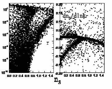
Figure 2: Models plotted in the $(n_{S},r)$ and $(n_{S},dn_{S}/d\ln{k})$ plane for an $M=8$ Monte Carlo. The number of e-folds is now randomly generated in range $\left[40,70\right]$.

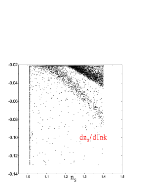
Figure 3: Models plotted in the $(n_{S},dn_{S}/d\ln{k})$ plane for a 10,000,000 simulation fitting into the window around 1$\sigma$ WMAP constraints at $k=0.002$ $Mpc^{-1}$. The cause of the straight line around $n_{S}=1$ can be found in Fig.7.

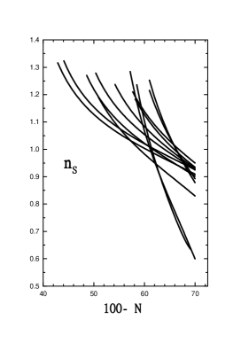
Figure 4: Twelve resulting spectral indices that runs significantly from blue to red, satisfying 1$\sigma$ WMAP constraintsWMAP2 .

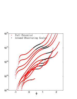
Figure 5: Twelve reconstructed inflaton potentials from Fig.4.

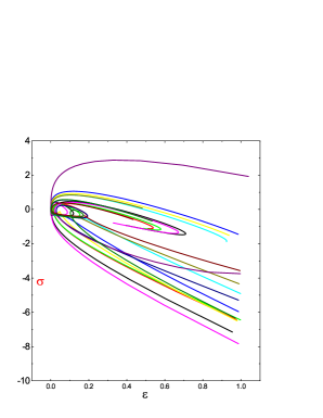
Figure 6: Twelve trajectories of $\epsilon$-$\sigma$ from Fig.4 during inflation.

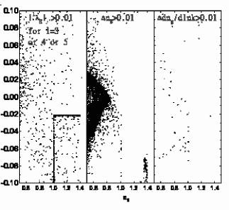
Figure 7: Crosscheck of SR approximations for a 10,000,000 simulation on the observable values of $n_{S}$ and $dn_{S}/d\ln k$, with $dn_{S}/d\ln k$ being the vertical axis. The left panel shows those which lead to wrong observable values due to nonegligible higher order effects of ${}^{l}\lambda_{\rm H}$ ($l\geq 3$); The middle and right panel show those which give wrong values of $n_{S}$ and $dn_{S}/d\ln k$ due to insufficient SR approximation to second order.

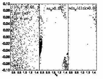
Figure 8: The same as Fig.7 for a 10,000,000 iteration on Method Crosscheck described in the text.

There have been in the literature several works which try to reconstruct inflaton potential using ideal observational datackll03 ; lidsey95 ; Ke03 . Generally speaking, first year WMAP data have not provided stringent window for one to constrain the inflaton potential. WMAP has not detected tensor contributions in the primordial spectrum: $r\leq 1$WMAP2 . This leads to $\epsilon\leq 0.07$ and hence $H^{2}\leq 4.8\times 10^{-10}m^{2}_{Pl}$, this gives $0<V\leq 5.8\times 10^{-11}m^{4}_{Pl}$ via the Hamilton-Jacobi equation. As also shown although a large running is favored, WMAP is consistent with scale invariant spectrum. Peiris et.al.WMAP2 categorized the slow roll parameters into four classes for generic single field inflaton potentials and found for either class there is broad region consistent with current observations. In this sense first year WMAP data (together with other observational data) have not been able to work as a stringent enough discriminator. As for the reconstructing method, there would be broad parametric space when the observational window is less stringent. However as the observational data accumulate and the error bar shrinks, e.g. when tensor contribution is exactly measured and running of the spectral index is strongly confirmed, reconstructing the favored inflaton potential would make its sense. On the inflationary flow itself, it would be inefficient since very small fraction fall into our window above, meanwhile most of the iterations fall into lat-time attractors and little part satisfies the window. In any case it provides a testable inflaton potential generator which may be exactly solvable. Liddleliddle03flow has made some detailed descriptions on its shortcomings: Firstly the flow equations (Eq.9 in this paper) do not relate directly to the inflationary dynamics. This should not be a severe problem since the reconstruction of potential needs using the Hamilton-Jacobi equation, where the dynamics is included. Secondly due to the truncation on $M-th$ order, the effective potential is only in such form

$$V(\phi) = \frac{3m_{{\rm Pl}}^{2}}{8\pi}\,H_{0}^{2}\left(1+A_{1}\phi+\cdots+A_{M+1}\phi^{M+1}\right)^{2}$$

$$\times\left[1-\frac{1}{3}\frac{m_{{\rm Pl}}^{2}}{4\pi}\left(\frac{A_{1}+\cdots+(M+1)A_{M+1}\phi^{M}}{1+A_{1}\phi+\cdots+A_{M+1}\phi^{M+1}}\right)^{2}\right]\,.$$

We made a detailed check and found the form is satisfied exactly. This in fact does accomodate many inflaton potentials as there are so many undecided parameters to choose and an ideally no truncation would accomodate all the single field inflaton potentials which satisfy above equation of motion and the Hamilton-Jacobi equation. A main loophole is pointed by Liddle liddle03flow that for the nontrivial points where inflation ends at $\epsilon=1$ the full potential is negative at its minimum. For example Eq.17 reduces to $V(\phi)=V_{0}((1+A_{1}\phi)^{2}-\frac{A_{1}}{12\pi})$ when only $\epsilon$ is nonzero where the flow equation starts to evolve (we set $\phi$ to be zero here). However as the flow equation only describes the dynamics of inflation at $\epsilon\leq 1$ where $V$ is always positive (as can be clearly seen from Eq.2 ), we can assume that the exact potential after inflation can be matched by other potentials which reach the minimum at $V=0$ (or arguably matched at $\epsilon=1$), the perturbations would certainly be the same as in Eq.17. In this sense flow equations can reconstruct potentials $during$ inflation. Similar arguments hold for the fixed points where inflaton reaches a local positive minimum and drives eternal inflation, this situation can be related to the standard hybrid inflation mechanismlinde91 ; linde94 , as shown by Easther and KinneyKe03 . In any case the flow equations seem to be inefficient as the inflaton potential generator when confronted with a large negative running from blue to red, which is around the 1$\sigma$ region of first year data of WMAP. Further investigation to find better infaton generator is necessary confronted with future precise observations.

So far we have left the second order SR approximation(SRA) undiscussed (We thank the anonymous referees for inspirations on this issue). It has been noted in the literaturehorder that higher order SR contributions may not be negligible especially when confronted with high precision observational data. This being the first time to check the precision of SR approximation in the framework of inflationary flow, we first rewrite the spectral index to the third order in the form of flow parameters(Basing on Refs.GStewart, ; STG01, ):

$$n_{S}-1 = \sigma+2\alpha{}^{2}\lambda_{\rm H}+\left(\alpha^{2}-\frac{\pi^{2}}{12}\right){}^{3}\lambda_{\rm H}+\left(4-12\alpha\right)\epsilon^{2}$$ (27)

$$+\left(3-5\alpha\right)\epsilon\sigma+\left(-5\alpha^{2}+8\alpha-6+\frac{5\pi^{2}}{12}\right)\epsilon~{}{}^{2}\lambda_{\rm H}$$

$$+\left(\frac{\alpha^{2}}{2}+4-\frac{13\pi^{2}}{24}\right)\sigma~{}{}^{2}\lambda_{\rm H}$$

$$+\left(6\alpha^{2}-32\alpha+28-\frac{\pi^{2}}{2}\right)\epsilon^{3}$$

$$+\left(-\frac{9}{2}\alpha^{2}-6\alpha-18+\frac{27}{8}\pi^{2}\right)\epsilon^{2}\sigma$$

$$+\left(-\frac{5}{2}\alpha^{2}+3\alpha-13+\frac{35}{24}\pi^{2}\right)\epsilon\sigma^{2}$$

where $\alpha=\frac{3-C}{4}=0.7296$. We made three sets of crosscheck in our 1000,000 and 10,000,000 iterations. Firstly one can see from Eq.18 the factors on ${}^{2}\lambda_{\rm H}$ and ${}^{3}\lambda_{\rm H}$ differ no more than five times. There being no efforts available in higher order SRA as Ref.GStewart, has explicitly did, we first make a strong limit that $max($ $\mid{}^{3}\lambda_{\rm H}\mid$, $\mid{}^{4}\lambda_{\rm H}\mid$, $\mid{}^{5}\lambda_{\rm H}\mid)<0.01$ (taken as Condition A)is satisfied. Those which violate this condition are plotted in the left panel of Fig.7. Other limits are taken to ensure that the values of $dn_{S}/d\ln k$ (taken as Condition B)and $n_{S}$ (taken as Condition C)differ no more than 0.01 when a third order SRA is assumed instead of second order SRA. They are delineated in the right and middle panels of Fig.7. To our great surprise 319, 134 and 6376 points violate Conditions A,B and C respectively in the 1000,000 iteration and for the 10,000,000 iteration 3089, 1404 and 64589 points violate the three conditions ( 751,215 total nontrivial points for the 10,000,000 iteration). That is to say, near ten percents of nontrivial points need to be reconsidered when a third order SRA is taken instead of second order SRA. A natural conclusion is that one has to take the order of SRA as high as possible to ensure the validity of SRA. It seems that we are lucky enough today- as can be seen from Fig.7- the regions where Conditions B and C are violated seems to be disfavored by current observations. For the stringent condition A we can find the straight lines in Figs.1,3 are due to the violation of this condition. It is however noted that Conditions B and C are the weak conditions which work only to third order and nothing could be ensured under fourth or fifth order SRA. Would this be the real case, one has to solve Eq.17 mode by mode instead. (A naive way out $might$ be to ensure the validity of decreasing sufficiently the higher order flow parameters.) It is worth mentioning again that the flow equations of Eq.9 is always exact under any order of truncation. In this sense the way of using flow equations like Ref.Dodelson, is appropriate, while many other papers in the literature suffer from second order SRAKinney02 ; Ke03 ; WMAP2 ; Kinney03 ; probflow . When a truncation to eighth order is considered instead we find similar results. For an iteration of 1000,000 points with truncation to the eighth order(Method Crosscheck) shown in Fig.2 we get 1,972, 289 and 5,216 points for models that violate Conditions A,B and C. A 10,000,000 iteration of Method Crosscheck is also tried and we get 17 insignificant points, 1,841 with $|{}^{\ell}\lambda_{\rm H}|>10^{8}$ and 757,521 nontrivial points. The 19,719, 2,804 and 51,626 points which violate Conditions A, B and C are shown in corresponding window in Fig.8. This seems to put current inflationary flow to considerable jeopardy.

In summary, the WMAP result of a varying spectral index, if further stands, could be used as a discriminator for inflationary models; most extant models would face a severe challenge. Using the inflationary flow equations, we have studied in this paper the possibility of reconstructing inflation models with large running spectral indices, which is favored by the WMAP analysis.

Acknowledgments: Firstly we shall thank the anonymous referees of this paper who inspired our thorough examination on the flow scenario. We thank Profs. Zuhui Fan, Jun’ichi Yokoyama and Xinmin Zhang for discussions and Drs. Xuelei Chen, Mingzhe Li, Bin Gong and Wanlei Guo for hospitable help. We acknowledge the using of Numerical RecipesPressBK1 . This work was supported in part by National Natural Science Foundation of China under Grant No. 10273017 and by Ministry of Science and Technology of China under Grant No. NKBRSF G19990754.

Table 1 – Twelve sets of initial flow parameters that lead to large running in the index as shown in Fig.4.

$\epsilon$	$\delta$	${}^{2}\lambda_{\rm H}$	${}^{3}\lambda_{\rm H}$	${}^{4}\lambda_{\rm H}$	${}^{5}\lambda_{\rm H}$
$0.10201$	$0.01683$	-0.03307	-0.02149	0.00575	$6.72964\times 10^{-4}$
$0.18937$	$-0.341$	-0.03109	-0.02458	0.00442	0.00183
$0.15207$	$-0.26372$	-0.03191	-0.01817	0.00386	0.00128
$0.07001$	$-0.4049$	-0.01344	-0.02067	0.01039	$-3.28768\times 10^{-5}$
$0.14667$	$-0.47786$	-0.03289	-0.02483	0.00687	0.00236
$0.08029$	$-0.00671$	-0.04361	-0.01302	0.0068	$-4.26084\times 10^{-5}$
$0.049$	$-0.16761$	0.03082	-0.02339	0.00379	$1.31775\times 10^{-4}$
$0.12419$	$-0.38872$	-0.01121	-0.01841	$6.05911\times 10^{-5}$	0.00274
$0.1241$	$0.08762$	0.0374	-0.02455	-0.00283	0.0017
$0.00532$	$-0.35618$	-0.00659	0.00402	0.0017	$1.77594\times 10^{-4}$
$0.16525$	$-0.39355$	-0.00507	-0.01349	$-6.855\times 10^{-4}$	0.00134
$0.16751$	$-0.40666$	-0.04769	-0.02294	0.00863	$7.67554\times 10^{-4}$

References

- (1) A. Kogut et al., Astrophys. J. Suppl. 148, 161 (2003).
- (2) D. N. Spergel et al., Astrophys. J. Suppl. 148, 175 (2003).
- (3) H. V. Peiris et al., Astrophys. J. Suppl. 148, 213 (2003).
- (4) W. J. Percival et al., Mon. Not. Roy. Astr. Soc. 327, 1297 (2001).
- (5) R. A. C. Croft et al., Ap. J. 581, 20 (2002); N. Y. Gnedin and A. J. S. Hamilton, Mon. Not. Roy. Astr. Soc. 334, 107 (2002).
- (6) U. Seljak, P. McDonald and A. Makarov, Mon.Not.Roy.Astron.Soc. 342, L79 (2003).
- (7) S. Smith et al., astro-ph/0401618; R. Rebolo et al., astro-ph/0402466; C. Dickinson et al., astro-ph/0402498;
- (8) B. Feng, M. Li, R.-J. Zhang, and X. Zhang, Phys. Rev. D 68, 103511 (2003).
- (9) J. E. Lidsey and R. Tavakol, Phys. Lett. B 575, 157 (2003); M. Kawasaki, M. Yamaguchi and J. Yokoyama, Phys.Rev. D 68, 023508 (2003); Q. G. Huang and M. Li, JHEP 0306, 014 (2003); D. J. Chung, G. Shiu and M. Trodden, Phys.Rev. D 68, 063501 (2003); K.-I. Izawa, Phys. Lett. B 576, 1 (2003); M. Bastero-Gil, K. Freese and L. Mersini-Houghton, Phys.Rev.D 68 (2003) 123514; M. Yamaguchi and J. Yokoyama, Phys.Rev.D 68 (2003) 123520; B. Wang, C. Lin and E. Abdalla, Phys.Rev.D 69 (2004) 063507; G.Dvali and S. Kachru, hep-ph/0310244; W. Lee, Y. Charng, D. Lee and L. Fang, astro-ph/0401269; M. Yamaguchi and J. Yokoyama, hep-ph/0402282; D. Lee, L. Fang, W. Lee and Y. Charng, astro-ph/0403055.
- (10) S. L. Bridle, A. M. Lewis, J. Weller, and G. Efstathiou, Mon.Not.Roy.Astron.Soc. 342, L72 (2003)
- (11) e.g. C. R. Contaldi, M. Peloso, L. Kofman, and A. Linde, JCAP 0307, 002 (2003); E. Gaztanaga et al, astro-ph/0304178; J. M. Cline, P. Crotty and J. Lesgourgues, JCAP 0309 (2003) 002; B. Feng and X. Zhang, Phys.Lett.B 570, 145 (2003); M. Kawasaki and F. Takahashi, Phys.Lett.B 570, 151 (2003); G. Efstathiou, Mon.Not.Roy.Astron.Soc. 346, L26 (2003); S. Tsujikawa, R. Maartens and R. Brandenberger, Phys.Lett. B 574, 141 (2003); T. Moroi and T. Takahashi, Phys.Rev.Lett. 92, 091301 (2004); Q. Huang and M. Li, JCAP 0311 001, (2003); X. Bi, B. Feng and X. Zhang, hep-ph/0309195; J.-P. Luminet et al, Nature 425 593, (2003); Y. Piao, B. Feng and X. Zhang, hep-th/0310206; Q. Huang and M. Li, astro-ph/0311378; L. R. Abramo and L. Sodre, astro-ph/0312124; Y. Piao, S. Tsujikawa and X. Zhang, hep-th/0312139; T. Multamaki and O. Elgaroy, astro-ph/0312534.
- (12) P. Mukherjee and Y. Wang, Astrophys.J. 599,1 (2003).
- (13) V. Barger, H. Lee, and D. Marfatia, Phys.Lett.B 565, 33 (2003); S. M.Leach and A. R.Liddle, Phys.Rev.D 68 (2003) 123508.
- (14) W. H.Kinney, E. W.Kolb, A. Melchiorri and A. Riotto, hep-ph/0305130;
- (15) M. B. Hoffman and M. S. Turner, Phys. Rev. D 64, 023506 (2001).
- (16) S. H. Hansen and M. Kunz, Mon. Not. Roy. Astron. Soc. 336, 1007 (2002).
- (17) W. H. Kinney, Phys. Rev. D 66, 083508 (2002).
- (18) S. Dodelson and L. Hui, Phys.Rev.Lett.91 131301, (2003)
- (19) R. Easther and W. H. Kinney, Phys. Rev. D 67, 043511 (2003).
- (20) A. R. Liddle, Phys. Rev. D 68, 103504 (2003).
- (21) A. R. Liddle, P. Parsons, and J. D. Barrow, Phys. Rev. D 50, 7222 (1994).
- (22) E. D. Stewart and D. H. Lyth, Phys. Lett. B 302, 171 (1993).
- (23) J. E. Lidsey, A. R. Liddle, E. W. Kolb, E. J. Copeland and T. Barreiro, Rev. Mod. Phys. 69, 373 (1997).
- (24) B. Feng, X. Gong and X. Wang, astro-ph/0301111.
- (25) E. J. Copeland, E. W. Kolb, A. R. Liddle and J. E. Lidsey, Phys. Rev. Lett. 71 219 (1993).
- (26) A. D. Linde, Phys. Lett. 259B, 38 (1991).
- (27) A. Linde, Phys. Rev. D 49 748 (1994).
- (28) e.g. D. H. Huang, W. B. Lin and X. M. Zhang, Phys. Rev. D 62, 087302 (2000); J. Martin and D. Schwarz, Phys. Rev. D 62, 103520 (2000); S. M. Leach, A. R. Liddle, J. Martin and D. J. Schwarz, Phys. Rev. D 66, 023515 (2002); X. Wang et al., astro-ph/0209242.
- (29) J. Gong and E. Stewart, Phys.Lett.B510 1, (2001).
- (30) D. J. Schwarz, C. A. Terrero-Escalante and A. A. Garcia, Phys. Lett. B 517, 243 (2001).
- (31) W. H. Kinney, astro-ph/0307005.
- (32) W. H. Press, S. A. Teukolsky , W. T. Vettering and B. P. Flannery, Numerical Recipes in FORTRAN, 2 ed. (Cambridge University Press, Cambridge, 1992).