Stellar evolution with rotation and magnetic fields:

We further develop the Tayler–Spruit dynamo theory, based on the most efficient instability for generating magnetic fields in radiative layers of differentially rotating stars. We avoid the simplifying assumptions that either the $\mu$– or the $T$–gradient dominates, but we treat the general case and we also account for the nonadiabatic effects, which favour the growth of the magnetic field. The general equation leads to the same analytical solutions in the limiting cases considered by Spruit (Spruit02 (2002)). Numerical models of a 15 M_⊙ star with a magnetic field are performed. The differences between the asymptotic solutions and the general solution demonstrate the need to use the general solution. Stars with a magnetic field rotate almost as a solid body. Several of their properties (size of the core, MS lifetimes, tracks, abundances) are closer to those of models without rotation than with rotation only. In particular, the observed N/C or N/H excesses in OB stars are better explained by our previous models with rotation only than by the present models with magnetic fields that predict no nitrogen excesses.

We show that there is a complex feedback loop between the magnetic instability and the thermal instability driving meridional circulation. Equilibrium of the loop, with a small amount of differential rotation, can be reached when the velocity $U_{\mathrm{magn}}$ of the growth of the magnetic instability is of the same order as the velocity $U_{\mathrm{circ}}$ of the meridional circulation. This opens the possibility for further magnetic models, but at this stage we do not know the relative importance of the magnetic fields due to the Tayler instability in stellar interiors.

tars: rotation – stars: magnetic field – stars: evolution

1 Introduction

A major concern is to know whether magnetic fields are important for stellar evolution or not (cf. Roxburgh Rox03 (2003)). Some initial numerical tests have suggested that the magnetic fields created by the Tayler–Spruit dynamo (Spruit Spruit99 (1999), Spruit02 (2002)) in rotating stars may be large enough to transport angular momentum in stellar interiors as well as chemical elements in upper MS stars (Maeder & Meynet Magn1 (2003)). In this work, we perform further theoretical developments of the dynamo process, as well as some numerical models, to study the consequences of stellar evolution with a magnetic field.

In the nice theory of magnetic instabilities recently developed by Spruit (Spruit02 (2002)), only some important limiting cases have been considered. In particular, the so–called Cases 0 and 1 have been studied. In Case 0, the $\mu$–gradient dominates over the thermal gradient in stellar interiors, i.e., in terms of the partial Brunt–Väisälä frequency we have $N_{\mu}>N_{\mathrm{T}}$. Case 1 applies when the thermal gradient is the main restoring force, i.e., when $N_{\mu}<N_{\mathrm{T}}$. In this case, the radiative losses from the magnetic instability are also accounted for; these losses reduce the restoring force of buoyancy which acts against the magnetic instability.

The problem with the above description is that, in the interiors of models no longer on the zero–age sequence, there is at some moderate distance of the core a significant zone with $N_{\mu}<N_{\mathrm{T}}$ (covering about 25 % of the stellar radius), which is in a situation where the current simplifications made in Case 1 are not appropriate. In this zone (we called it zone 1P), the magnetic instability is adiabatic, while the hypothesis of large non-adiabaticity is made (see Sect. 2 below). It also happens in all stars that there are zones where $N_{\mu}$ and $N_{\mathrm{T}}$ are of the same order and where it is better to account for both gradients, even if in general such zones are rather small. We consider it preferable to consistently treat the general case and to account properly everywhere for the $T$– and $\mu$–gradients, as well as for the non–adiabatic effects.

Also, the two approximations mentioned above have very different functional dependences with respect to stellar parameters, such as the angular velocity $\Omega$, the differential rotation $q=-\frac{\partial\ln\Omega}{\partial\ln r}$ or the thermal and chemical gradient. The use of asymptotic solutions such as Spruit’s (Spruit02 (2002)) introduces artificial jumps in the behaviour of the diffusion coefficients.

Our purpose here is to express the theory in a unique and consistent formulation for all possible cases of $N_{\mu}$ and $N_{\mathrm{T}}$ and of departures from adiabaticity. In Sect. 2, we discuss the non–adiabaticity as a function of radiative and magnetic diffusivities $K$ and $\eta$ respectively. In Sect. 3, we establish the general equations for the magnetic field and we check for consistency with the expressions derived by Spruit (Spruit02 (2002)). In Sect. 4 we examine the general expressions for the transport of the angular momentum and of the chemical elements. Sect. 5 shows some initial numerical applications as an example. In Sect. 6 we examine the reciprocal feedback between meridional circulation and Tayler instability and the fact that these two processes lead to very different amounts of differential rotation. The conclusions are given in Section 7.

2 The radiative heat losses of the magnetic instability

2.1 Magnetic diffusivity and radiative losses

As shown by Spruit (Spruit02 (2002)), the magnetic diffusivity $\eta$ in Case 0 ($N_{\mu}>N_{\mathrm{T}}$) is given by

$$\eta_{\mathrm{0}}=r^{2}\;\Omega\;\left(\frac{\omega_{\mathrm{A}}}{\Omega}\right)^{4}\left(\frac{\Omega}{N_{\mu}}\right)^{2}\;,$$ (1)

while in Case 1 ($N_{\mu}<N_{\mathrm{T}}$), it is given by

$$\eta_{\mathrm{1}}=r^{2}\;\Omega\;\left(\frac{\omega_{\mathrm{A}}}{\Omega}\right)^{2}\left(\frac{\Omega}{N_{\mathrm{T}}}\right)^{\frac{1}{2}}\left(\frac{K}{r^{2}N_{\mathrm{T}}}\right)^{\frac{1}{2}}\;.$$ (2)

The Alfvén frequency $\omega_{\mathrm{A}}$ is given by

$$\omega_{\mathrm{A}}=\frac{B}{(4\pi\rho)^{\frac{1}{2}}\;r}\;.$$ (3)

The Brunt–Väisälä frequency, when the $\mu$–gradient dominates over the T–gradient, tends towards the following partial frequency

$$N_{\mu}^{2}\;=\;\frac{g\varphi}{H_{\mathrm{P}}}\nabla_{\mu}\;,$$ (4)

and when the T–gradient dominates, it tends towards

$$N_{\mathrm{T}}^{2}\;=\;\frac{g\delta}{H_{\mathrm{P}}}(\nabla_{\mathrm{ad}}-\nabla)\;.$$ (5)

The thermodynamic coefficients $\delta$ and $\varphi$ are defined as follows: $\delta=-\left(\frac{\partial\ln\rho}{\partial\ln T}\right)_{\mathrm{P},\mu}$ and $\varphi=\left(\frac{\partial\ln\rho}{\partial\ln\mu}\right)_{\mathrm{T,P}}$. $H_{\mathrm{P}}$ is the pressure scale height. We need a general expression for the magnetic diffusivity encompassing the two limiting cases with $\eta_{\mathrm{0}}$ and $\eta_{\mathrm{1}}$. This requires further study of the nonadiabatic heat losses. For a fluid element displaced over a length $l$, the thermal fluctuations diffuse with a timescale $t_{\mathrm{therm}}\approx\frac{l^{2}}{K}$, where $K$ is the thermal diffusivity $K=\frac{4acT^{3}}{3\kappa\rho^{2}C_{\mathrm{p}}}$. Let us call $t$ the typical timescale over which the magnetic instability develops. In a time $t$, the fluctuations are reduced by a factor $f$, which can be written (cf. Spruit Spruit02 (2002)),

$$f\;=\;\frac{t}{t_{\mathrm{therm}}}+1\;.$$ (6)

If $f\rightarrow 1$ as for $t_{\mathrm{therm}}\gg t$, where t is the dynamical timescale of the instability, one has the adiabatic case. On the other hand, if $f\rightarrow\infty$ as for $t_{\mathrm{therm}}\ll t$, we have a highly nonadiabatic case. Spruit (Spruit02 (2002)) also introduces in Case 1 (when $N_{\mathrm{T}}$ dominates) an “effective thermal buoyancy frequency” $N_{\mathrm{e}}=\frac{N_{\mathrm{T}}}{f^{\frac{1}{2}}}$ and assumes $t_{\mathrm{therm}}\ll t$. This implies that $f\simeq\frac{t}{t_{\mathrm{therm}}}$. If it happens in some stellar layer that $t\ll t_{\mathrm{therm}}$, the situation is adiabatic and one should have $f=1$, but the adopted simplification leads to $f=0$. The approximation is thus invalid in this case.

The factor $f$ introduced by Spruit is related to the usual Peclet number $P_{\mathrm{e}}=\frac{t_{\mathrm{therm}}}{t_{\mathrm{dyn}}}\simeq\frac{v\;l}{K}$, which is the ratio of the thermal to the dynamical timescales for a fluid element of velocity $v$ displaced over a length $l$. In astrophysics, rather than the Peclet number, one often considers (e.g. in the theory of convection) a factor $\Gamma$, which is the ratio between the energy delivered by a fluid element to the energy lost during the displacement of the fluid element. For a typical geometry, i.e., by assuming that the fluid elements are spherical, one would have $\Gamma=\frac{1}{6}\;P_{\mathrm{e}}$. The fluid elements are likely not spherical in the relevant geometry for Tayler instability. We should rather consider thin slabs of thickness $l$, (we are indebted to Henk Spruit for this remark). If so, the relation between $\Gamma$ and the Peclet number is $\Gamma=\frac{1}{2}\;P_{\mathrm{e}}$. Thus, the following relation is valid for the factor $f$ introduced by Spruit and the usual number ratios $P_{\mathrm{e}}$ or $\Gamma$

$$\Gamma=\frac{1}{2}\;\frac{1}{(f-1)}\quad\quad\mathrm{or}\quad f\;=\;\frac{1\;+\;2\;\Gamma}{2\;\Gamma}\;.$$ (7)

This comes directly from the abovementioned definition of the Peclet number as well as from Eq. (6). In the adiabatic case, $f\rightarrow 1$ and $\Gamma\rightarrow\infty$; if non–adiabatic effects are important, $f$ is large and $\Gamma$ is very small.

2.2 Oscillations frequencies

The general expression of the Brunt–Väisälä frequency for a displaced fluid element is

$$N^{2}=\frac{g\;\delta}{H_{\mathrm{P}}}(\nabla^{\prime}-\nabla+\frac{\varphi}{\delta}\nabla_{\mu})\;,$$ (8)

where $\nabla^{\prime}$ is the internal gradient of the the fluid element,i.e., expressing how $T$ changes inside the fluid element during its motion, while $\nabla$ is the T–gradient of the surrounding medium. One also has the following relations between the various $T$–gradients (cf. Maeder Maeder95 (1995))

$$\nabla^{\prime}-\nabla=\frac{\Gamma}{\Gamma+1}(\nabla_{\mathrm{ad}}-\nabla)\;$$ (9)

and

$$\nabla=\frac{\nabla_{\mathrm{rad}}+\frac{2\;\Gamma^{2}}{1+\Gamma}\nabla_{\mathrm{ad}}}{1+\frac{2\;\Gamma^{2}}{1+\Gamma}}\;,$$ (10)

with a numerical factor of 6 instead of 2, if we would have considered spherical fluid elements. Thus, in a radiative zone where there is some motion of matter, which may be non–adiabatic, the thermal gradient depends on the efficiency $\Gamma$ of the thermal transport and the gradient may lie anywhere between the adiabatic and radiative gradients depending on this efficiency. If we write $\Gamma$ in terms of $f$, we have

$$\frac{\Gamma}{\Gamma+1}=\frac{1}{2f-1}\;.$$ (11)

Thus, we may also write the Brunt–Väisälä frequency taking account of radiative losses in terms of $f$, as follows

$$N^{2}=\frac{1}{2f-1}N^{2}_{\mathrm{T}}+N^{2}_{\mu}\;.$$ (12)

When $N_{\mu}=0$, Spruit (Spruit02 (2002)) writes $N^{2}_{\mathrm{e}}=\frac{N^{2}_{\mathrm{T}}}{f}$, which has a dependence on $1/f$ for large values of $f$; however we note that the numerical factors may introduce some differences.

We can go a step further in expressing $\Gamma$ in term of the ratio $\eta/K$ of the magnetic to the thermal diffusivity. As seen above, one has $\Gamma\simeq\frac{1}{2}\;\frac{l^{2}}{t\;K}$, where $l$ is the length scale of the instability. Instabilities over smaller lengthscales are removed by magnetic diffusivity. We consider here the marginal case $l^{2}=\eta\;t$ (cf. Spruit Spruit02 (2002)) and thus we get

$$\Gamma=\frac{1}{2}\;\frac{\eta}{K}\;.$$ (13)

Thus, one obtains the ratio $\frac{\Gamma}{\Gamma+1}=\frac{\eta}{\eta\;+\;2K}$, which leads to the following expression for the Brunt–Väisälä frequency

$$N^{2}=\frac{\eta/K}{\eta/K+2}\;N^{2}_{\mathrm{T}}+N^{2}_{\mu}\;.$$ (14)

This is the oscillation frequency of a fluid element displaced by Tayler–Spruit instability. The numerical factor of $2$ in the above expression is due to the geometry we considered; in many cases this numerical factor will introduce some minor differences with to Spruit (Spruit02 (2002)). The resulting differences will be rather small because this factor will generally appear with a power smaller than $1$, as for example in Eq. (35).

3 General equation for the magnetic diffusivity

As emphasized by Spruit (Spruit02 (2002)), the energy of the Tayler instability (Tayler Tay73 (1973)) must be large enough to overcome the restoring force of buoyancy and this implies that the Alfvén frequency must be larger than some limit. Thus, the vertical extent $l_{\mathrm{r}}$ of the magnetic instability must be limited (cf. Spruit Spruit02 (2002), Eq. 6),

$$l_{\mathrm{r}}<\frac{r\;\omega_{\mathrm{A}}}{N}\;.$$ (15)

However, if this radial scalelength is too small, the perturbations will be quickly damped by the diffusion of the magnetic field characterized by $\eta$ and this implies $l_{\mathrm{r}}^{2}>\frac{\eta}{\sigma_{\mathrm{B}}}$, where $\sigma_{\mathrm{B}}$ is the characteristic frequency of the magnetic field. In the absence of Coriolis force, this frequency is $\sigma_{\mathrm{B}}=\omega_{\mathrm{A}}$. However, as shown by Spruit (Spruit02 (2002); see also Pitts & Tayler Pitts86 (1986)), in a rotating star (typically when $\Omega>\omega_{\mathrm{A}}$) this frequency becomes $\sigma_{\mathrm{B}}=(\omega_{\mathrm{A}}^{2}/\Omega)$ due to the Coriolis force. Therefore one has in this case

$$l_{\mathrm{r}}^{2}>\frac{\eta}{\sigma_{\mathrm{B}}}=\frac{\eta\;\Omega}{\omega_{\mathrm{A}}^{2}}\;.$$ (16)

The combination of these two limits together with Eq. (14) leads to the following condition $\left(\frac{\omega_{\mathrm{A}}}{\Omega}\right)^{4}>\frac{N^{2}}{\Omega^{2}}\;\frac{\eta}{r^{2}\;\Omega}$, where $N^{2}$ is given by Eq. (14). For the marginal situation corresponding to equality, we have

$$\left(\frac{\omega_{\mathrm{A}}}{\Omega}\right)^{4}=\frac{N^{2}}{\Omega^{2}}\;\frac{\eta}{r^{2}\;\Omega}\;.$$ (17)

This equation relates the two unknown quantities, the magnetic diffusivity $\eta$ and the Alfvén frequency $\omega_{\mathrm{A}}$.

For the particular cases studied by Spruit (Spruit02 (2002)), the result was a much simpler equation. Here, we find it preferable to establish a second relation between the two unknown quantities. The amplification time $\tau_{\mathrm{a}}$ of the Tayler–Spruit instability, i.e., “the timescale on which the radial field $B_{\mathrm{r}}$ is amplified into an azimuthal field of the same order as the already existing azimuthal field” can be written $\tau_{\mathrm{a}}=N/(\omega_{\mathrm{A}}\Omega q)$ (Spruit Spruit02 (2002)). The equality of the two timescales $\tau_{\mathrm{a}}$ and $\sigma_{\mathrm{B}}^{-1}$, according to the expression given above, leads to a second equation $\frac{\omega_{\mathrm{A}}}{\Omega}=q\;\frac{\Omega}{N}$, as found by Spruit (Spruit02 (2002); his Eq. 18). When account is taken of the expression of the Brunt–Väisälä (Eq. 14), this gives

$$\left(\frac{\omega_{\mathrm{A}}}{\Omega}\right)^{2}=\frac{\Omega^{2}\;q^{2}}{N^{2}_{\mathrm{T}}\;\frac{\eta/K}{\eta/K\;+\;2}+N^{2}_{\mu}}.$$ (18)

The above two equations (17, 18) form a coupled system of degree 4 (see below) with two unknown quantities, $\eta$ and $\omega_{\mathrm{A}}$. This system could be solved by standard procedures, however we first make some simplifications. We eliminate the expression of $N^{2}$ between these two equations and obtain

$$\eta\;=\;\frac{r^{2}\;\Omega}{q^{2}}\;\left(\frac{\omega_{\mathrm{A}}}{\Omega}\right)^{6}\;.$$ (19)

This is a new general equation connecting the magnetic diffusivity and the Alfvén frequency. It shows that the Alfvén frequency, and therefore the magnetic field, changes as 1/6 the power of the magnetic diffusivity for a given rotation. This coefficient applies to the diffusion of the azimuthal component of the magnetic field. Due to the particular pinch–type nature of the Tayler–Spruit instability, it also applies to the turbulent diffusive mixing of the chemical elements by this instability. To ensure consistency, we verify that in Spruit’s Case 0 with

$$\left(\frac{\omega_{\mathrm{A}}}{\Omega}\right)^{2}_{0}=\left(q\;\frac{\Omega}{N_{\mu}}\right)^{2}\;,$$ (20)

we get

$$\eta_{0}=r^{2}\Omega q^{4}\;\left(\frac{\Omega}{N_{\mu}}\right)^{6}\;.$$ (21)

This is in agreement with Eq. (42) by Spruit (Spruit02 (2002)). This equation shows that the mixing of chemical elements decreases very strongly if the $\mu$–gradient grows and this effect limits the chemical mixing of elements by the Tayler–Spruit dynamo in the regions just above the convective core.

In Case 1, when thermal losses are accounted for, the Alfvén frequency is given by

$$\left(\frac{\omega_{\mathrm{A}}}{\Omega}\right)_{1}=q^{\frac{1}{2}}\left(\frac{\Omega}{N_{\mathrm{T}}}\right)^{\frac{1}{8}}\left(\frac{K}{r^{2}N_{\mathrm{T}}}\right)^{\frac{1}{8}}\;$$ (22)

This is given by Spruit (Spruit02 (2002); his Eq. 19). Below, we will verify that our system of equations also leads to this expression (see Eq. 35 below). For now, we check that our Eq. (19) with this expression of $(\frac{\omega_{\mathrm{A}}}{\Omega})_{1}$ leads to

$$\eta_{1}=r^{2}\Omega\;q\left(\frac{\Omega}{N_{\mathrm{T}}}\right)^{\frac{3}{4}}\left(\frac{K}{r^{2}N_{\mathrm{T}}}\right)^{\frac{3}{4}}\;,$$ (23)

which is the same as Eq. (43) by Spruit (Spruit02 (2002)). Thus, we have checked the consistency of the general expression for $\eta$ (Eq. 19) with the results obtained by Spruit (Spruit02 (2002)) in the two particular cases he considered. There are no new physics here with respect to Spruit’s work (Spruit02 (2002)), we simply verify the consistency of our general expression with the asymptotic cases considered by Spruit.

Now, we can introduce the general expression of $\eta$ given by (19) in the second equation (Eq. 18) of our coupled system and obtain

$$\left(\frac{\omega_{\mathrm{A}}}{\Omega}\right)^{2}\left[N_{\mathrm{T}}^{2}\;\frac{r^{2}\Omega}{q^{2}K}\left(\frac{\omega_{\mathrm{A}}}{\Omega}\right)^{6}+N_{\mu}^{2}\;\left(\frac{r^{2}\Omega}{q^{2}K}\left(\frac{\omega_{\mathrm{A}}}{\Omega}\right)^{6}+2\right)\right]=$$

$$\left(\frac{r^{2}\Omega}{q^{2}K}\;\left(\frac{\omega_{\mathrm{A}}}{\Omega}\right)^{6}+2\right)\;\Omega^{2}\;q^{2}.\quad\quad\;$$ (24)

Since the ratio $\left(\frac{\omega_{\mathrm{A}}}{\Omega}\right)$ always appears with a power of 2, we now define a new variable $x=\left(\frac{\omega_{\mathrm{A}}}{\Omega}\right)^{2}$ and thus we get

$$\frac{r^{2}\Omega}{q^{2}K}\left(N_{\mathrm{T}}^{2}+N_{\mu}^{2}\right)x^{4}-\frac{r^{2}\Omega^{3}}{K}x^{3}+2N_{\mu}^{2}\;x-2\Omega^{2}q^{2}=0\;.$$ (25)

We have transformed our system of two equations of degree 4 with two unknown quantities $\eta$ and $\omega_{\mathrm{A}}$ into one equation of degree 4 with only one unknown quantity $x$. The solution will provide the value of the Alfvén frequency and the magnetic diffusivity $\eta$ by Eq. (19). Higher order terms depending on $\Gamma=\frac{1}{2}\frac{\eta}{K}$ might be considered, but as also shown by Spruit, this ratio is very small. The above equation applies to the general case where both $\nabla_{\mu}$ and $N_{\mathrm{T}}$ are different from zero and where thermal losses may reduce the restoring buoyancy force. This full equation is to be solved numerically (see Sect. 5 below).

Higher order terms depending on $\Gamma^{2}$ could be considered, but it is correct to limit the development to the first order in $\Gamma$. Indeed, we notice that the expression of $N_{\mathrm{T}}$ given by Eq. (5) contains the term $\nabla$, which is given by Eq. (10). This term $\nabla$ contains the ratio $\eta\over K$. If we would fully develop the above equation taking this additional dependence into account we would get an equation of order 10 instead of order 4 as above. We remark that the dependence in $\eta\over K$ introduced by $\nabla$ in the expression of $N^{2}$ is of an higher order in $\eta\over K$ than the one expressed by Eq. (14). Since $\eta\over K$ ranges between $10^{-2}$ and $10^{-7}$ in the numerical models of Sect. 5, we may ignore this higher order term.

We can also check that Eq. (25) leads to simple solutions fully consistent with the results by Spruit (Spruit02 (2002)) in the particular cases he has studied:

– 1. Firstly, we notice that if terms going like the power 6 or higher of $\left(\frac{\omega_{\mathrm{A}}}{\Omega}\right)$ are negligible, the solution is simply

$$x=\left(q\;\frac{\Omega}{N_{\mu}}\right)^{2}\;,$$ (26)

which is the same as Eq. (20) above. This is the so–called Case 0. Indeed, the condition $\omega_{\mathrm{A}}\ll\Omega$ leads to a solution which is the same as when $N_{\mathrm{T}}=0$, which defines Case 0.

– 2. The general Eq. (25) can also be written

$$\frac{r^{2}\Omega}{K}x^{3}\left(\frac{x}{q^{2}}(N_{\mathrm{T}}^{2}+N_{\mu}^{2})-\Omega^{2}\right)+2q^{2}\left(\frac{xN_{\mu}^{2}}{q^{2}}-\Omega^{2}\right)=0\;.$$ (27)

We notice some similarity of the two terms in parentheses. If we consider Spruit’s Case 0 with $N_{\mathrm{T}}=0$, this equation becomes the product of two terms

$$\left(\frac{x}{q^{2}}N_{\mu}^{2}-\Omega^{2}\right)\left(\frac{r^{2}\Omega}{K}x^{3}+2q^{2}\right)=0\;.$$ (28)

The solutions are

$$x=\frac{q^{2}\Omega^{2}}{N_{\mu}^{2}}\quad\quad\mathrm{and}\quad x^{3}=-\frac{2\;q^{2}K}{r^{2}\Omega}\;.$$ (29)

The second possibility leads to negative solutions, which are thus not physically meaningful. Thus, this shows the uniqueness of the first solution.This first solution is that of Case 0, given above by Eq. (20), as found by Spruit (Spruit02 (2002)).

– 3. Let us consider Case 1 with $N_{\mu}=0$. We have from Eq. (27)

$$\frac{r^{2}\Omega}{K}x^{3}\left(\frac{x}{q^{2}}N_{\mathrm{T}}^{2}-\Omega^{2}\right)-2\;q^{2}\Omega^{2}=0\;.$$ (30)

If $q$ is small, one has the solution

$$x=\frac{q^{2}\Omega^{2}}{N^{2}_{\mathrm{T}}}\;,$$ (31)

which is the alternative solution proposed by Spruit(Spruit02 (2002)), when the simplification resulting from the assumption of a large $f$ value does not apply, (this is the case we have called 1P).

We may also examine the general solution when the ratio $\eta/K$ is small, which is generally the case as seen above and as mentioned by Spruit. For that, we start from the two equations (17, 18) and make the simplifications appropriate for a small $\eta/K$ ratio. With developments like those done above, we get instead of Eq. (25) the following expression

$$\frac{r^{2}\Omega}{q^{2}K}N_{\mathrm{T}}^{2}\;x^{4}+2N_{\mu}^{2}\;x-2\;\Omega^{2}q^{2}=0\;,$$ (32)

which is similar to our Eq. (25) for $N_{\mu}=0$, except that the term in $x^{3}$ has disappeared. Indeed, we may also derive the above equation directly from our general Eq. (25) by noting that if $\eta/K$ is small, then from Eq. (18) one has

$$x=\frac{\Omega^{2}\;q^{2}}{N^{2}_{\mu}}$$ (33)

and then by multiplying this equation by $\frac{x^{3}r^{2}\Omega N^{2}_{\mu}}{q^{2}K}$, we get

$$x^{4}\frac{r^{2}\;\Omega}{q^{2}\;K}N_{\mu}-\frac{r^{2}\;\Omega^{3}}{K}\;x^{3}=0\;.$$ (34)

When we bring this relation into Eq. (25), we are lead to the above Eq. (32). Thus, this relation (32) is fully consistent with our general equation.

In Case 1 when $N_{\mu}$, the above Eq. (32) leads to

$$\left(\frac{\omega_{\mathrm{A}}}{\Omega}\right)=2^{\frac{1}{8}}\;q^{\frac{1}{2}}\left(\frac{\Omega}{N_{\mathrm{T}}}\right)^{\frac{1}{4}}\left(\frac{K}{r^{2}\Omega}\right)^{\frac{1}{8}}=$$

$$2^{\frac{1}{8}}\;q^{\frac{1}{2}}\left(\frac{\Omega}{N_{\mathrm{T}}}\right)^{\frac{1}{8}}\left(\frac{K}{r^{2}N_{\mathrm{T}}}\right)^{\frac{1}{8}}\;.$$ (35)

This is just the same expression, except for the small geometrical factor $2^{\frac{1}{8}}$, as in the equation found by Spruit (Spruit02 (2002), i.e.,his Eq. 19).

Thus, for all situations considered by Spruit, we have verified here that our general equations (19, 25) well reproduce his results.

4 Transport of angular momentum and chemical elements

Let us specify some other useful expressions such as the critical lengthscale for the Spruit–Tayler instability, the intensity of the magnetic field, the coefficients of transport for the angular momentum and for the chemical elements. As shown above, the vertical extent of the magnetic instability is limited by $l_{\mathrm{r}}<\frac{r\;\omega_{\mathrm{A}}}{N}$ (Eq. 15), where N is given by the general expression (14). Thus the maximum lengthscale of the magnetic instability is

$$l_{r}=\frac{r\;\omega_{\mathrm{A}}}{\left(\frac{\eta/K}{\eta/K+2}\;N^{2}_{\mathrm{T}}+N^{2}_{\mu}\right)^{\frac{1}{2}}}\;.$$ (36)

Following Spruit (Spruit02 (2002)), we consider this maximal value as the one charateristic, for example, of mixing, since the mixing will be essentially determined by the instabilities with the longest lengthscale. We immediately verify that $l_{r}$ is in agreement with Spruit’s (Spruit02 (2002)) result in Case 0, when $N_{\mathrm{T}}=0$. In Case 1, when $N_{\mu}=0$, we may write, if we assume in addition that $\frac{\eta}{K}$ is small,

$$l_{r}=\frac{r\;\omega_{\mathrm{A}}}{\left(\frac{\eta}{2K}\right)^{\frac{1}{2}}N_{\mathrm{T}}}\>.$$ (37)

With the general expression of $\eta$ given by Eq. (19), this becomes

$$l_{\mathrm{r}}=\frac{2^{\frac{1}{2}}\;K^{\frac{1}{2}}\;q\;\Omega^{\frac{5}{2}}}{N_{\mathrm{T}}\;\omega_{\mathrm{A}}^{2}}\;.$$ (38)

With Eq. (35) for $\omega_{\mathrm{A}}$, we get finally in Case 1

$$l_{\mathrm{r}}=2^{\frac{1}{4}}\;r\;\left(\frac{\Omega}{N_{\mathrm{T}}}\right)^{\frac{1}{2}}\left(\frac{K}{r^{2}\Omega}\right)^{\frac{1}{4}}\;,$$ (39)

which is identical to the result by Spruit (Spruit02 (2002); Eq. 10), apart from the geometrical factor $2^{\frac{1}{4}}$. Thus, our general expression for the lengthscale $l_{\mathrm{r}}$ of the Tayler–Spruit instability also contains the limiting cases studied by Spruit. We also recall, as shown in Eq. (12) by Spruit, that $\eta\ll K$ is a condition of validity for the developments made by Spruit.

Turning now to the general expression for the intensity of the magnetic field, following Spruit (Spruit02 (2002)) we have for the azimuthal and radial field strengths,

$$B_{\varphi}=(4\pi\rho)^{\frac{1}{2}}\;r\;\omega_{\mathrm{A}}\quad\mathrm{and}\quad B_{\mathrm{r}}=B_{\varphi}\;(l_{\mathrm{r}}/r)\;.$$ (40)

The quantity $\omega_{\mathrm{A}}$ has to be taken as the solution of the general equation (25) and $l_{\mathrm{r}}$ is given by Eq. (36). These general expressions also reproduce correctly the particular Cases 0 and 1, since we have verified the consistency of our general expressions for $l_{\mathrm{r}}$ and $\omega_{\mathrm{A}}$ with those for the two particular cases. For Case 0, this gives (cf. Spruit (Spruit02 (2002)),

$$B_{\varphi}=(4\pi\rho)^{\frac{1}{2}}r\;q\frac{\Omega^{2}}{N_{\mu}}\;,\quad\mathrm{and}\quad\frac{B_{\mathrm{r}}}{B_{\varphi}}=\;q\left(\frac{\Omega}{N_{\mu}}\right)^{2}\;.$$ (41)

For Case 1, one has

$$B_{\varphi}=2^{\frac{1}{8}}(4\pi\rho)^{\frac{1}{2}}\;r\;\Omega\;q^{\frac{1}{2}}\left(\frac{\Omega}{N_{\mathrm{T}}}\right)^{\frac{1}{8}}\left(\frac{K}{r^{2}\;N_{\mathrm{T}}}\right)^{\frac{1}{8}}$$ (42)

and

$$\frac{B_{\mathrm{r}}}{B_{\varphi}}=2^{\frac{1}{4}}\left(\frac{\Omega}{N_{\mathrm{T}}}\right)^{\frac{1}{4}}\left(\frac{K}{r^{2}\;N_{\mathrm{T}}}\right)^{\frac{1}{4}}\;.$$ (43)

These last two expressions are identical to those by Spruit except for the geometrical factors $2^{\frac{1}{8}}$ and $2^{\frac{1}{4}}$ respectively.

Let us now turn towards the transport of angular momentum by the magnetic field. The azimuthal stress by volume unity due to the magnetic field is given by

$$S\;=\frac{1}{4\;\pi}\;B_{\mathrm{r}}B_{\varphi}\;=\;\frac{1}{4\;\pi}\;\left(\frac{l_{\mathrm{r}}}{r}\right)B_{\varphi}^{2}=\;\rho\;r^{2}\;\left(\frac{\omega_{\mathrm{A}}^{3}}{N}\right)\;.$$ (44)

Following the ingenious procedure devised by Spruit (Spruit02 (2002)), we can express the viscosity $\nu$ for the vertical transport of angular momentum in terms of $S$. Indeed, the viscosity of a fluid represents its ability to transport momentum from one place to another and thus we get,

$$\nu=\frac{S}{\rho\;q\;\Omega}=\;\frac{\Omega\;r^{2}}{q}\;\left(\frac{\omega_{\mathrm{A}}}{\Omega}\right)^{3}\;\left(\frac{\Omega}{N}\right)\;.$$ (45)

This is the general expression of $\nu$ with $\omega_{\mathrm{A}}$ given by the solution of Eq. (25) and with $N$ by Eq. (14). We immediately verify that in Case 0 with $\frac{\omega_{\mathrm{A}}}{\Omega}=\;q\;\frac{\Omega}{N_{\mu}}$, we find the same as Spruit (Spruit02 (2002)),

$$\nu_{0}=r^{2}\;\Omega\;q^{2}\;\left(\frac{\Omega}{N_{\mu}}\right)^{4}\;.$$ (46)

The $\mu$–gradient, through its reduction of the field, particularly in the vertical direction, also reduces the transport of angular momentum, but much less than for the chemical elements as given by Eq. (21). In Case 1, it is also easy to verify, by using the appropriate expressions for N, $l_{\mathrm{r}}$ and $\omega_{\mathrm{A}}$ that one obtains,

$$\nu_{1}=2^{\frac{1}{2}}r^{2}\;\Omega\;\left(\frac{\Omega}{N_{\mathrm{T}}}\right)^{\frac{1}{2}}\left(\frac{K}{r^{2}N_{\mathrm{T}}}\right)^{\frac{1}{2}}\;,$$ (47)

which is identical to Eq. (32) by Spruit (Spruit02 (2002)) apart from the geometrical factor $6^{\frac{1}{2}}$.

Thus, we have the full set of expressions necessary to obtain the Alfvén frequency $\omega_{\mathrm{A}}$, the magnetic diffusivity $\eta$, which is necessary for calculating the transport of the chemical elements, and the viscosity $\nu$ for the vertical transport of the angular momentum by the magnetic field. These expressions apply to the general case, where both the $\mu$– and $T$–gradients are different from zero and where radiative losses may play a role. In all cases, the general expressions may also lead consistently to the asymptotic expressions by Spruit (Spruit02 (2002)). We may remark that we need not to include here the erosion of the $\mu$–gradient by the horizontal turbulence as suggested by Talon & Zahn (TalonZ (1997)), since as shown by Maeder & Meynet (Magn1 (2003)), the horizontal turbulence is either suppressed or at least strongly reduced by the magnetic field.

Figure 1: Internal distribution of the angular velocity $\Omega(r)$ as a function of the radius in solar units in the model V3 (without magnetic field) at various stages of the model evolution indicated by the central H–content $X_{\mathrm{c}}$ during the MS–phase. The initial mass is 15 M_⊙ and $Z=0.02$.

Figure 2: Internal distribution of the angular velocity $\Omega(r)$ as a function of the radius in solar units in the model M1 (with magnetic field calculated according to Spruit Spruit02 (2002)) at various stages of the model evolution indicated by the central H–content $X_{\mathrm{c}}$ during the MS–phase. The initial mass is 15 M_⊙ and $Z=0.02$.

Finally, let us check consistency. The rate of magnetic energy production $W_{\mathrm{B}}$ per unit of time and volume must be equal to the rate $W_{\nu}$ of the dissipation of rotational energy by the magnetic viscosity $\nu$ as given above. This check of consistency is verified for the asymptotic expressions, but we have to see whether the general expressions also fulfill it. We assume here that the whole energy dissipated is converted to magnetic energy, which is a reasonable approximation. The sink of energy due to chemical mixing is negligible here, since as shown below the transport of elements from the core to the surface is absent from models with the magnetic field as calculated here.

$$W_{\nu}={1\over 2}\rho\nu\Omega^{2}q^{2},$$ (48)

which gives with Eq. (45),

$$W_{\nu}={1\over 2}\rho\;q\;r^{2}\frac{\Omega}{N}\omega_{\mathrm{A}}^{3}\;.$$ (49)

With Eq. (18) defining the field amplitude $\left(\frac{\omega_{\mathrm{A}}}{\Omega}\right)=\frac{\Omega\;q}{N}$, the dissipation rate finally becomes

$$W_{\nu}={1\over 2}\rho r^{2}q^{4}\Omega^{3}\left(\frac{\Omega}{N}\right)^{4}\;.$$ (50)

We turn to the rate $W_{\mathrm{B}}$ of magnetic energy creation. The magnetic energy per unit volume is $\frac{B^{2}}{8\pi}$, it is produced in a characteristic time given by $\sigma_{\mathrm{B}}^{-1}=(\omega_{\mathrm{A}}^{2}/\Omega)^{-1}$. Thus, one has

$$W_{\mathrm{B}}=\frac{B^{2}}{8\pi}\frac{\omega_{\mathrm{A}}^{2}}{\Omega}=\frac{1}{2}\rho r^{2}\frac{\omega_{\mathrm{A}}^{4}}{\Omega}\;,$$ (51)

where we have used the Eq. (40) for the field, because $B_{\varphi}$ is the main field component. If we now use the above expression of $\frac{\omega_{\mathrm{A}}}{\Omega}$, we get the same expression as for $W_{\nu}$ (Eq. 50), thus one has

$$W_{\nu}\;=\;W_{\mathrm{B}}.$$ (52)

This shows the consistency of the field expression for $B_{\varphi}$, of the transport coefficient $\nu$ together with the energy conservation in the process of field creation.

5 Numerical applications

5.1 Existing models, present models and their aims

Figure 3: Internal distribution of the angular velocity $\Omega(r)$ as a function of the radius in the model M5 (with magnetic field calculated according to expressions of the present paper) at various stages of the model evolution indicated by the central H–content $X_{\mathrm{c}}$ during the MS phase. The dotted line shows the values at the end of the H–burning phase.

Many sets of models with rotation exist, often without magnetic fields. A general review of the models without magnetic field has been made by Maeder & Meynet (MMaraa (2000)) and more recent references are given in the recent IAU Symposium 215 on Stellar Rotation (Maeder & Eenens MEe (2004)). Most models cover the H– and He–burning phases, while some models go up to the pre–supernova stage (Heger et al. HegerI (2000); Hirschi et al. Hirschi04 (2004)). The models often differ significantly in their physical assumptions and the way they are modelized. A particularly critical point is the treatment of the meridional circulation, which in many sets of recent models is treated as a diffusion process, which is incorrect since a diffusion process goes along the gradient of the considered quantity (for example $\Omega$), while the advection due to meridional circulation may transport the angular momentum from the location where there is less (central regions) to the location where there is more (superficial regions), and it can also do the opposite depending on the circulation patterns.

Several stellar models with rotation and magnetic fields have been published in the recent literature. The interaction between meridional circulation and dynamo action have been studied by Charbonneau & MacGregor (Charb01 (2001); see also Sect. 6 below). Heger et al. (Heger04 (2004)) have implemented Spruit’s (Spruit02 (2002)) asymptotic developments in models of stellar evolution. These authors follow from the ZAMS to the pre-supernovae stage the evolution of the specific angular momentum. They find in particular that the models with magnetic field lead to neutron stars spinning about an order of magnitude slower than the models without magnetic field by Heger et al. (HegerI (2000). The model with magnetic field is still rotating faster than observed in young pulsars, while it is to slow for making the collapsar model possible (Woosley Woosley93 (1993); MacFadyen et al. MacF01 (2001)). The effect of magnetic field in the core collapse have been studied by Fryer & Warren (FryerW04 (2004)), who find that magnetic fields do not play a dominant role in the supernova explosion mechanism.

In paper I of this series (Maeder & Meynet Magn1 (2003)), we have calculated a model of a 15 M_⊙ with solar composition and an initial rotation velocity $v_{\mathrm{ini}}$ of 300 km s^-1. At a stage near the middle of the MS phase, we have examined what happens if we “turn on” the magnetic field and apply Spruit’s expressions (Spruit Spruit02 (2002)). The general result was that both the transports of angular momentum and of chemical elements by Tayler magnetic instability was much larger than the transports by meridional circulation and shear instability. Thus, this leads us to suspect that magnetic field is an important component of stellar evolution.

Figure 4: Evolution of the rotation velocities at the surface of the various models with an initial mass of 15 M_⊙ with $Z=0.02$, during the MS phase. The heavy broken line is for model V3 the light broken–line for model M1 and the continuous line for model M5.

Here, we want to compare Spruit’s solutions and the more general developments expressions developed here. Also, we want to study the effects of the field through the evolution. For that purpose, we follow the MS evolution of 4 different types of models of 15 M_⊙ with solar composition. These models are labeled as follows:

• V0: a model with no rotation and no magnetic field.

• V3: a model with $v_{\mathrm{ini}}=300$ km$\cdot$s^-1, and no magnetic field, with the physical assumptions adopted by Meynet & Maeder (MMX (2000)) except for the overshooting parameter which was taken here equal to 0.

• M1: a model with $v_{\mathrm{ini}}$ of 300 km$\cdot$s^-1 and with magnetic field calculated according to the expressions given by Spruit (Spruit02 (2002)), i.e., for Case 0 when $N_{\mu}>N_{\mathrm{T}}$ and for Case 1 when $N_{\mu}<N_{\mathrm{T}}$. In Case 1, when the account of radiative losses does not increase the magnetic diffusivity, another case called 1P as given by Eq. (31) is considered (Spruit Spruit02 (2002)).

• M5: a model with $v_{\mathrm{ini}}$ of 300 km$\cdot$s^-1 and with magnetic field according to the expressions of the present paper.

In both models M1 and M5, we did not include the effects of meridional circulation and horizontal turbulent diffusion, since these effects were found small with respect to those due to the magnetic field, (see remarks in Sect. 6). In these first basic tests, overshooting and semiconvection were not included. However, we keep the effects of shear mixing and the hydrostatic effects of rotation, which distort the equipotentials and modify the stellar shape, which has great consequences on the $T_{\mathrm{eff}}$ of rotating models. To make the comparisons more relevant, we do not include in model M5 the energy condition discussed in paper I, since this condition was not included by Spruit (Spruit02 (2002)). Some further theoretical works are still needed about this condition and this point will be examined in a further work.

5.2 Evolution of the internal and superficial rotation

We examine the evolution of the internal profile of $\Omega(r)$ in the various models. Figs. 1, 2 and 3 show these profiles at various evolutionary stages during the evolution of models V3, M1 and M5 respectively. In model V3, we notice the smooth, but significant decline of $\Omega(r)$ outside the convective core, where rotation is homogeneous. Such an evolution of rotation has been studied in detail by Meynet & Maeder (MMV (2000)) and Maeder & Meynet (MMVII (2001)) at solar composition and at lower metallicity. The angular velocity is first decreasing in the core as mass loss removes angular momentum at stellar surface, because enough coupling of rotation is ensured by shear mixing and meridional circulation to largely compensate the acceleration of rotation which would result from the moderate core contraction. Only at the end of the MS phase, central rotation increases due to the dominant effect of central contraction. In the outer layers, a smooth but significant decrease of rotation between the core and the surface is created by the abovementioned processes.

Figure 5: Internal distribution of the hydrogen mass fraction $X$ as a function of the Lagrangian mass in the model V3 (with rotation only) at various stages of the model evolution from top to bottom during the MS–phase.

Figure 6: Internal distribution of the hydrogen mass fraction $X$ as a function of the Lagrangian mass in the model M5 (with magnetic field calculated according to expressions of the present paper) at various stages of the model evolution from top to bottom during the MS–phase.

In Fig. 2 and 3, we notice several interesting new facts for models with a magnetic field:

• The models have almost an internal solid body rotation, with a difference of only a few percent between the core and the bulk of the envelope, with a short transition at their interface. The differential rotation parameter $q$ is very small, but still different from zero. The relative constancy of $\Omega$ is the result of the high value of the transport coefficient $\nu$ by the magnetic field (see below Fig. 8). We notice that these results are in agreement with those of Heger et al. (Heger04 (2004)), who also find essentially solid body rotation until the end of the MS phase. Then in later phases, differential rotation appears together with a slowing down of the core.

• There is a general slowing down of rotation during evolution due to two effects: the mass loss which removes angular momentum and the expansion of the external layers. The strong internal coupling of rotation transports this slowing down to the core.

• Models M1 and M5, although not strictly identical (see Fig. 4), exhibit similar $\Omega$–distributions.

• We notice a small decrease of $\Omega$ near the surface. This is likely resulting from the expansion of the superficial layers after the removal of some mass by stellar winds at the surface.

Fig. 4 shows the evolution of the surface velocities for models V3, M1 and M5. We note the small differences between models M1 and M5, showing that the general treatment is not identical to Spruit’s solutions. We see that the fast initial decline of model V3, due to the rapid adjustment of an equilibrium profile by meridional circulation (cf. Meynet & Maeder MMV (2000)) is absent in models with magnetic field which rotate nearly like a solid body from the ZAMS onwards. Thus models M1 and M5 keep an almost constant surface velocity, while model V3 also has a slight decline during the rest of the MS phase. Very likely this behaviour is different for different initial masses, because of the differences in the mass loss rates. Thus, a complete grid has to be made in order to establish a basis for comparisons with the observations.

5.3 Internal distribution of hydrogen

The evolution of the internal distribution of hydrogen mass fraction is illustrated in Fig. 5 for model V3 and in Fig. 6 for model M5 with magnetic field, (models M1 and M5 gives very similar curves with only minor differences as illustrated by the evolution of the core sizes in Fig. 9). We see that at the end of the MS phase model M5 produces a convective core which is slightly smaller than for model V3. The H–distribution outside the core is much smoother in model V3: there is more helium outside the formal core of this model than in model M5. The reason is that in the magnetic models the transport of chemical elements is strongly inhibited by the $\mu$–gradient just outside the core: the diffusion coefficient for chemical elements depends on $N_{\mu}$ with a power $-6$, as shown by Eq. (21). In the models with only rotation, the inhibition by $N_{\mu}$ for the shear diffusion goes like a power $-2$. The fact that more helium is burnt in models V3 has some consequences for the shape of the tracks in the HR diagram and also for the lifetimes as shown in Sect. 5.6 below.

Figure 7: Internal distribution of the partial Brunt–Väisälä frequencies $N^{2}_{\mathrm{T}}$ and $N^{2}_{\mu}$ for the model M5 at an age of $8.384\cdot 10^{6}$ yr with central H–content given by $X_{\mathrm{c}}=0.30$.

5.4 The Brunt–Väisälä and Alfvén frequencies

Fig. 7 shows the terms $N^{2}_{\mathrm{T}}$ and $N^{2}_{\mu}$ of the Brunt–Väisälä frequency for the model M5 near the middle of the MS phase, (the general behaviour is similar for model M1, thus we do not show it). We see that the thermal component $N^{2}_{\mathrm{T}}$ dominates through most of the envelope while the mean molecular weight component $N^{2}_{\mu}$ is much more important close to the core. This large $N^{2}_{\mu}$ inhibits the chemical mixing.

The ratio $\omega_{\mathrm{A}}/\Omega$ lies everywhere between $10^{-3}$ and $10^{-2}$. The magnetic field $B_{\varphi}$ is nearly constant through the star. Its amplitude is about $\log B_{\varphi}=4.4$ throughout with average deviations smaller than about 0.1 dex, where the field $B_{\varphi}$ is expressed in Gauss. As already suggested by Maeder & Meynet (Magn1 (2003)), the field currently due to Tayler–Spruit dynamo is rather large in massive stars. The situation is different here from the above work. The new point here is that even the equilibrium field is large, i.e., the field created by the differential rotation which is itself strongly reduced by the field in a consistent feedback. The magnetic field decreases fastly near the stellar surface, because differential rotation becomes negligible. What is left of the field in the photosphere is difficult to ascertain without more detailed models. Also, we recall that for consistency with Spruit’s equations (Spruit02 (2002)), we have not accounted here for the energy condition proposed in paper I (Maeder & Meynet Magn1 (2003)), which tends to reduce or suppress the field in the outer layers.

5.5 Diffusion coefficients for the transports of the angular momentum and chemical elements

Figure 8: Internal distribution of the coefficients of diffusion. The coefficient $\nu$ (Eq. 45) for the transport of angular momentum by the magnetic field is shown by the continuous line. The coefficient of transport of the chemical elements, i.e., the magnetic diffusivity $\eta$ given by Eq. (19) is shown by a short–dashed line. The coefficient $D_{\mathrm{shear}}$ of the shear turbulent mixing is shown in comparison as a dotted line. The long–dashed line shows the thermal conductivity $K$. The ages of the models are the same as in the model of Fig. 7.

Fig. 8 shows the coefficients of transport in model M5. The continuous, higher curves represent the coefficient $\nu$ for the transport of the angular momentum as given by Eq. (45). In the outer layers, the value of $\nu$ reaches about $10^{15}$ cm${}^{2}\cdot$ s^-1, which differs by less than one order of magnitude from the typical values of the diffusion coefficient in a convective zone. In the region where the $\mu$–gradient becomes significant, the diffusion is reduced to $\nu\approx 10^{9}$ cm${}^{2}\cdot$s^-1, which is still large. These values of $\nu$ implies a strong coupling of the rotation motions, which is responsible for the near constancy of the angular velocity $\Omega$ through the whole stellar interior. As illustrated by Eq. (45) and (46), this coefficient behaves like $(\Omega/N_{\mu})^{4}$ in this region, which explains the observed decline towards the interior. This decline is also favoured by the fact that $N^{2}_{\mathrm{T}}$ also decreases towards the deep interior as illustrated by Fig. 7. We see that $\nu$ and the thermal diffusivity $K$ are of the same order of magnitude in the region above the core, while $\nu$ is larger in the outer layers. This behaviour is consistent with the comparison (cf. Table 1 below) of the velocities of meridional circulation and of the growth of the magnetic instability.

Figure 9: The evolution of the mass of the convective core. The dotted–line applies to model V0, the long–broken (upper) line to model V3, the short–broken line to model M1, the continuous line to model M5.

The coefficient of magnetic diffusivity $\eta$, which acts both for the diffusion of the magnetic field as well as for the transport of the chemical elements as discussed in Sect. 3, is shown by the dashed–line in Fig. 8. Close to the core, the dependence of $\eta_{0}$ (Eq. 21) goes with the power of $-6$ on $N_{\mu}$. This explains why in the deep interior, near the core, this coefficient becomes very low, being less than $10^{3}$ cm${}^{2}\cdot$ s^-1. These regions where $\eta$ is very small tend to inhibit the transfer of the chemical elements towards the surface The coefficient $\eta$ grows rapidly in the very outer layers, rising up to $10^{12}$ cm${}^{2}\cdot$ s^-1. We may check here the very small values of the ratio $\eta\over K$ mentioned above.

A curve with coefficient $D_{\mathrm{shear}}$ due to shear turbulence is also shown in Fig. 8. As we have seen, the $\Omega$–gradient is not strictly zero. The value of $D_{\mathrm{shear}}$ is negligible in the outer layers, while it is larger than the coefficient for magnetic transport $\eta$ in the layers close to the core. The reason is that the dependence in $N_{\mu}$ is weaker for $D_{\mathrm{shear}}$ than for $\eta$, (being in $N_{\mu}^{-2}$ for the first and in $N_{\mu}^{-6}$ for the second). This means that both shear mixing and magnetic effects have to be taken into account. It is clear that the interaction of shear instability and magnetic field may be rather complex physically with some important feedback effects, particularly in regions where $D_{\mathrm{shear}}$ and $\eta$ are of the same order. The present work does not solve this point, but Fig. 8 shows the orders of magnitude of the main parameters. The main conclusion is that magnetic coupling dominates the dynamics of rotation. This conclusion is in agreement with that by Heger et al.(Heger04 (2004)), who also find an essentially solid body during MS evolution. We also notice that from a different physical dynamo model MacDonald & Mullan (MacD04 (2004)) suggest that shear instability is present over most of the interior, a result which possibly supports the simultaneous consideration of shear transport and magnetic field.

5.6 Evolution of the core, lifetimes and tracks in the HR diagram

Fig. 9 shows the evolution of the mass of the convective core. As well known, rotation produces an increase of the core mass fraction and of the MS lifetime. Here, the MS lifetime of model V3 is about 20 % larger than for model V0. The models M1 and M5 with both rotation and magnetic field have a core size and a MS lifetime which are intermediate between those of models V0 and V3, but closer to the non–rotating model V0. This is consistent with the results of Figs. 5 and 6, which show that there is more H burnt in models with rotation only. The mixing of the chemical elements by Tayler instability increases only very slightly the fuel reservoir with respect to a model without rotation, since the strong inhibition (Eq. 19) by the $\mu$–gradient limits very much the importance of the mixing. Again, we notice some small differences between models M1 and M5. The core is larger in M1 than in M5. The reason is likely due to the slightly larger values of $D_{\mathrm{shear}}$ in model M1 close to the core. The deviation of model M5 from the non–rotating case is very small: the lifetime is increased by only 2.4 %.

Fig. 10 shows the evolutionary tracks in the HR diagram. In interpreting these tracks, one must remember that the effects of the distortion of the stellar surface by rotation have been accounted for in the definition of the $T_{\mathrm{eff}}$. (In models with rotation, we define the average effective temperature as the stellar luminosity divided by the real distorted surface of the rotating star, cf. Meynet & Maeder MMI (1997)). This definition is equivalent to seeing the star with an average orientation, i.e., with an angle $i$ between the rotation axis and the line of sight equal to the root of the second Legendre polynomial, i.e., about 54 degrees. This is why all models with rotation start their evolution at a place in the HR diagram, which is different from that of the model V0 with no rotation.

Figure 10: Evolutionary tracks in the HR diagram. The dotted line refers to model V0, the long–broken line to model V3, the short–broken line to model M1 and the continuous line to model M5.

Model V3 experiences a larger increase of its luminosity than model V0, as a result of the more extended mixing and larger core as shown in Fig. 5. The growth of luminosity for models M1 and M5 is smaller than for model V3, because mixing is less extended (cf. Fig. 6). Models M1 and M5 experience about the same increase in luminosity as model V0. The end of the MS in these two models is a bit more shifted to the red by the atmospheric distortion than the zero–age models, since the ratio $\Omega\over\Omega_{\mathrm{c}}$ increases from about 0.66 to 0.82 during MS evolution.

We see a difference of the tracks for models M1 and M5. A rough agreement is achieved with the limiting cases by Spruit (Spruit02 (2002)), but the differences are not entierly negligible. We also notice the “stair–case” track of the magnetic models, particularly for model M1. This is the result of the rather particular evolution of the core mass of this model as illustrated in Fig. 9: initially model M1 evolves close to the model V3 with rotation, then it behaves more as the model V0 with no rotation, account being given to the atmospheric effect. This behaviour is rather different for model M5 which evolves like the model without rotation. This illustrates the different results obtained from the asymptotic relations and the general solution.

5.7 Evolution of the abundances of helium and CNO elements at the stellar surface

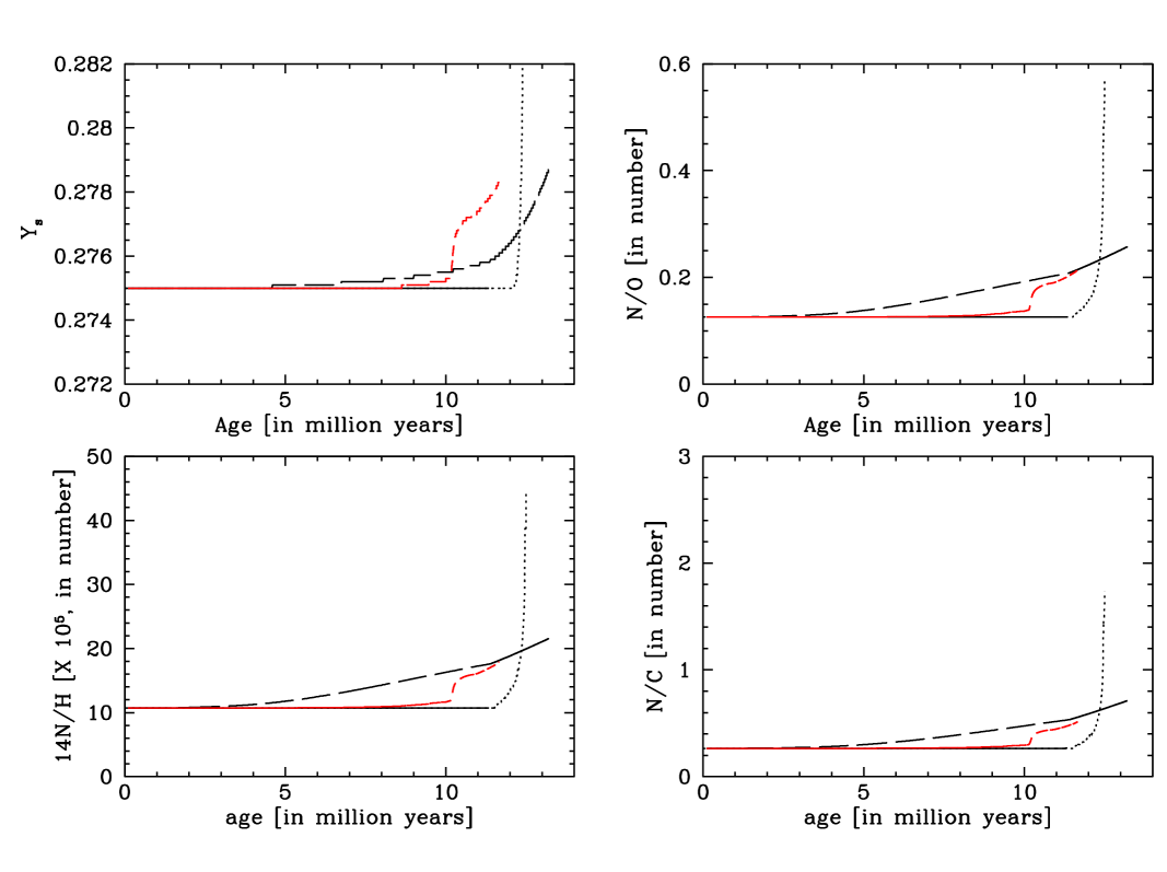
Figure 11: Time evolution of the surface helium content $Y_{\mathrm{s}}$ in mass fraction, of the N/O, N/H and N/C in mass fraction for the various models V0 (dotted line), V3 (long–broken line), M1 (short–broken line) and M5 (continuous line).

Fig. 11 reflects the evolution of the abundances of helium and CNO elements at the surface of the various models. For model V0, as is well known the enrichment only occurs when convective dredge–up appears in the red–supergiant stage. For model V3, the growth of the nitrogen at the stellar surface amounts to about a factor of 2 during the MS phase, as a result of shear mixing mainly and of meridional circulation to a smaller extent. The growth of the helium content is quite small and amounts to about 0.004 in $Y_{\mathrm{s}}$. Model M1 shows a late N–enrichment up to the level of model V3 near the end of the MS, while it is negligible before. The helium enhancement is even higher than for model V3. The striking point is that model M5 shows no enrichment at all. This is likely a consequence of slightly lower $D_{\mathrm{shear}}$ close to the core than for model M1. There the difference between models M1 and M5 is rather critical in view of the observational tests to be performed.

We know from spectroscopic observations that significant surface enrichments in helium and nitrogen occur in rotating O–stars as well in some early B–type stars (cf. Howarth & Smith Howarth01 (2001); Villamariz et al. Villamariz02 (2002)). Thus, the fact that the rotating model M5 does not produce such enrichments is a negative indication, suggesting that the present models with magnetic field do not well correspond to reality. The fact that the agreement is better realized with model M1 is not meaningful, since this results from the use of asymptotic relations which lead to an overestimate of the diffusion coefficients in some parts of the star. Incidentally, this also shows that wrong conclusions could be drawn, if the general expressions are not used. The models with only rotation much better agree with observations (cf. for example Maeder & Meynet MMVII (2001)). However, one must be careful. These comparisons do not necessarily exclude the presence of any magnetic fields playing a role in massive stars. In that respect, the remarks made in Sect. 6 below on the equilibrium reached between meridional circulation and magnetic transport certainly leads to more differential rotation and mixing than in the present models.

6 Discussion: interaction between Spruit’s dynamo and meridional circulation.

The aim of this section is to discuss the role of the magnetic field with respect to other instabilities, in particular the thermal instability, a point which has generally not been considered. The various authors, for example Heger et al. (Heger04 (2004)), usually just sum up the various effects. This simple approach may nevertheless have the interest to show the order of magnitude of the effects considered. When differences of several orders of magnitude appear between, for example, the coefficients for the transport of angular momentum $\nu$ and $D_{\mathrm{shear}}$, we may likely reach a conclusion about which effect dominates. In this context, we recall that Charbonneau (Charb01 (2001)) has examined the delicate interplay between dynamo and meridional circulation. With a different dynamo model, he has concluded that the dynamo action remains probable in presence of meridional circulation. Our conclusion below is not different. If only a dynamo is present, the star reaches solid body rotation, which would drive a circulation. On the contrary, we will see that, if we ignore the dynamo, the meridional circulation and star evolution build a differential rotation sufficient to make the dynamo active. Therefore, we may conclude that in the time evolution both effects of dynamo and meridional circulation are present, with a delicate balance between them. This first approach nevertheless still leaves room for a thorough analysis of the magnetic and thermal instabilities at a fundamental level.

We have seen in paper I (Maeder & Meynet Magn1 (2003)) that, if in the course of evolutionary models calculated with only the current effects of rotation (hydrostatic effects, meridional circulation, shear mixing, horizontal turbulence, etc…) and which have a significant amount of differential rotation, we estimate the magnetic field created by Tayler–Spruit dynamo, then the magnetic field and its transport effects are found to be very large. The transport coefficients $\nu$ and $\eta$ by the magnetic field were found to overcome the above mentioned effects of rotation, in particular meridional circulation which is usually the most important process for the transport of angular momentum. This lead us to suggest that magnetic fields may be dominating. The situation is probably not so simple.

In Sect. 5 above, we have followed the evolution of a 15 M_⊙ star with the magnetic field created by the Tayler–Spruit dynamo and we have found an internal equilibrium of rotation characterized by a nearly constant $\Omega(r)$ in the stellar interior due to the strong magnetic coupling expressed by the coefficient $\nu$. We may now wonder whether in these models with $\Omega\approx const.$ the effects of the magnetic field are always larger than those which could be due to the thermal instability driving meridional circulation. If the answer is “yes”, then clearly Tayler–instability and magnetic fields largely dominate the thermal instability responsible for meridional circulation. If on the contrary the answer is “no”, this means that the situation is more complicated.

The above worry is quite justified, since we know that there are various feedback mechanisms playing a role in the problem. Models with only rotation lead to a strong differential rotation, which in turn may feed the dynamo mechanism and the build–up of a magnetic field, which then would tend to dampen the differential rotation, which is its source. We also know from previous work (Meynet & Maeder MMV (2000)) that if rotation is constant in the interior, as is the case in the initial stellar models on the ZAMS, then the thermal instability and the resulting velocity $U(r)$ of meridional circulation is much larger than in the case for the equilibrium profile $\Omega(r)$ of rotation. Moreover $U(r)$ is positive everywhere in the envelope. This means that angular momentum is transported from the outer regions of the star to the inner ones, counterbalancing the effects of the transport by diffusion. Thus this large meridional circulation will enhance differential rotation. The complete feedback loop is the following, with two parts A and B:

A) Build–up of magnetic field and constant rotation:

differential rotation$\quad\Rightarrow\quad$dynamo$\quad\Rightarrow\quad$
     magnetic field$\quad\quad\;\quad\Rightarrow\;\;\Omega\sim const.$

B) Build–up of circulation and differential rotation:

$\Omega\sim const.\quad\;\Rightarrow\quad$stronger thermal instability$\quad\Rightarrow$
    higher $U(r)$$\quad\;\Rightarrow\quad$differential rotation$\quad\Rightarrow$ …

The basic equation governing the evolution of $\Omega(r)$ is the equation describing the conservation of the angular momentum, which is in Lagrangian coordinates (cf. Zahn, Zahn92 (1992); Maeder & Zahn MZ98 (1998))

$$\frac{d}{dt}\left(\rho r^{2}\overline{\Omega}\right)_{M_{r}}=\frac{1}{5r^{2}}\frac{\partial}{\partial r}\left(\rho r^{4}\overline{\Omega}U(r)\right)$$

$$\qquad+\frac{1}{r^{2}}\frac{\partial}{\partial r}\left(\rho\;\nu\;r^{4}\frac{\partial\overline{\Omega}}{\partial r}\right)\;.$$ (53)

$\overline{\Omega}(r)$ is the average angular velocity on the equipotential. If an equilibrium of the above feedback loop is reached in a time relatively short with respect to the evolutionary timescale, this equation is equal to zero. We would thus have a balance of the flux due to meridional circulation $U(r)$ by the flux due to the magnetic diffusion expressed by $\nu$, as shown by Eq. (53).The equilibrium is achieved for

$$U(r)=\;5\;\frac{\nu}{r}\;\left(-\frac{\partial\ln\Omega}{\partial\ln r}\right)\;.$$ (54)

The factor 5 results from the integration of the angular momentum over the isobar, which leads to the above Eq. (53). On the right side of Eq. (54), we have a velocity which can be associated with the magnetic diffusion. Let us call it $U_{\mathrm{magn}}$ and the left member $U_{\mathrm{circ}}$ to make the distinction. In Table 1, we compare the values of $U_{\mathrm{magn}}$ and $U_{\mathrm{circ}}$ at the middle of the MS phase in the model of 15 M_⊙ studied in Sect. 5.

Table 1: Comparison between $U_{\rm circ}$ and $U_{\rm magn}$ in a 15 M_⊙ model at X${}_{\rm{c}}=0.30$.

$M_{r}/M_{\odot}$	$U_{\rm circ}$	$\nu$	$|q|$	$\log r$	$U_{\rm magn}$
8.02	1.97e-02	2.03e+11	0.45e-3	11.1060	3.60e-03
10.05	1.55e-02	2.24e+12	0.62e-4	11.1897	4.46e-03
13.04	1.85e-02	7.78e+13	0.49e-4	11.3298	9.00e-02

We see that $U_{\mathrm{circ}}$ dominates over $U_{\mathrm{magn}}$ in the deep envelope, while the opposite situation occurs closer to the surface; the difference reaches about a factor of 5. Models with only rotation as in paper I indicate that the magnetic fields should be large, while models with magnetic fields as here indicate that the meridional circulation is significant. The basic reason for the difference is the $\Omega(r)$ profile, with important differential rotation in the first case and constant rotation in the second.

We think that an equilibrium profile of $\Omega(r)$ is reached as a result of the interaction of the two effects, neither with as much differential rotation as in the models with rotation only (cf. Fig. 1), nor with a constant angular velocity as in the present models with magnetic field (cf. Figs. 2 and 3). This intermediate $\Omega(r)$ profile will lead to more mixing than in the present case. Will this be enough to be in agreement with the observations? We do not know yet. We emphasize that the equilibrium profile of $\Omega(r)$ is likely defined by a particular balance between $U_{\mathrm{magn}}$ and $U_{\mathrm{circ}}$, with account taken also of the stellar contraction and angular momentum conservation. There is probably an additional constraint imposed by the fact that the energy of the magnetic field originates from the excess energy in differential rotation and thus the energy density in the magnetic field is limited by its energy source. Such effects will be examined in further work.

7 Conclusions

The equations for the general case of the Tayler–Spruit dynamo with $\mu$–gradients and nonadiabatic effects have been developed. The general expressions consistently allow us to recover Spruit’s asymptotic relations (Spruit02 (2002)), when $N_{\mu}$ or $N_{\mathrm{T}}$ are zero. Numerically the general and asymptotic results are consistent with some quantitative differences. This demonstrates the need to use the general solutions, in particular if we want to perform observational tests.

Some initial results on the role of possible magnetic field in stellar models have been found. The Tayler–Spruit dynamo imposes that the stars to rotate nearly as a solid body. This leads to a different evolution of rotational velocities as stars move away from the zero–age sequence. In general, the rotation velocities are higher when a magnetic field is present. A second general result is that internal mixing and surface enrichments in products of the CNO burning are smaller when a magnetic field is present than in rotating models without a magnetic field. Since spectroscopic observations of OB stars show significant N– and He–enrichments, this cast some doubt as to whether magnetic fields have a dominant effect, especially more than the models which have only rotation and no magnetic field show a good agreement with observations.

If magnetic fields are present, we may expect, as shown in Sect. 5, that the magnetic instability and the thermal instability which drives meridional circulation reach some balance in their complex feedback loop. For reasons explained in Sect. 5, this balance should be characterized by less differential rotation than in current models with only rotation and by more differential rotation than in the present models with a magnetic field. Such models may lead to more mixing than the present ones.

Finally, we emphasize that at this stage we really do not know how the Tayler–Spruit instability interacts with the meridional circulation and how the energy constraints may modify the results. But we have explored some consequences of the magnetic field in the absence of meridional circulation and examined the possibilities for its existence.

References

- (1) Charbonneau, P. & MacGregor, K.B. 2001, ApJ 559, 1094
- (2) Fryer, C.L., Warren, M.S. 2004, ApJ 601, 391
- (3) Heger, A., Langer, N., Woosley, S.E. 2000, ApJ 528, 368
- (4) Heger, A., Woosley, S.E., Langer, N., Spruit, H.C. 2004, in Stellar Rotation, IAU Symposium 215, Eds. A. Maeder & P. Eenens, in press.
- (5) Hirschi, R., Meynet, G., Maeder, A. 2004, A&A, submitted
- (6) Howarth, I. & Smith, K.C. 2001, MNRAS 327, 353
- (7) MacDonald, J., Mullan, D.J. 2004, MNRAS 348, 702
- (8) MacFadyen, A., Woosley, S.E., Heger, A. 2001, ApJ 550, 410
- (9) Maeder, A. 1995, A&A 199, 84
- (10) Maeder, A., Eenens, P. 2004, Stellar Rotation, IAU Symp. 215, ASP, in press.
- (11) Maeder, A., Meynet, G. 2000, ARA&A 38, 143
- (12) Maeder, A., Meynet, G. 2001, A&A 373, 555 (paper VII)
- (13) Maeder, A., Meynet, G. 2003, A&A 411, 543
- (14) Maeder, A., Zahn, J.P. 1998, A&A 334, 1000
- (15) Meynet, G., Maeder, A. 1997, A&A 321, 465 (paper I)
- (16) Meynet, G., Maeder, A. 2000, A&A 361, 101 (paper V)
- (17) Meynet, G., Maeder, A. 2003, A&A 404, 975 (paper X)
- (18) Pitts, E., Tayler, R.J. 1986, MNRAS 216, 139
- (19) Roxburgh, I. W. 2004, in Stellar Rotation, IAU Symp. 215, Eds. A. Maeder & P. Eenens, ASP Publ., in press.
- (20) Spruit, H.C. 1999, A&A 349, 189
- (21) Spruit, H.C. 2002, A&A 381, 923
- (22) Talon, S., Zahn, J.P. 1997 , A&A 317, 749
- (23) Tayler, R.J. 1973, MNRAS 161, 365
- (24) Villamariz, M.R., Herrero, A., Becker, S.R., Butler, K. 2002, A&A, 388, 940
- (25) Woosley, S.E. 1993, ApJ 405, 273
- (26) Zahn, J.P. 1992, A&A 265, 115