The Deep Lens Survey Transient Search I : Short Timescale and Astrometric Variability

Abstract

We report on the methodology and first results from the Deep Lens Survey (DLS) transient search. We utilize image subtraction on survey data to yield all sources of optical variability down to 24^th magnitude. Images are analyzed immediately after acquisition, at the telescope and in near–real time, to allow for followup in the case of time–critical events. All classes of transients are posted to the web upon detection. Our observing strategy allows sensitivity to variability over several decades in timescale. The DLS is the first survey to classify and report all types of photometric and astrometric variability detected, including solar system objects, variable stars, supernovae, and short timescale phenomena. Three unusual optical transient events were detected, flaring on thousand–second timescales. All three events were seen in the $B$ passband, suggesting blue color indices for the phenomena. One event (OT 20020115) is determined to be from a flaring Galactic dwarf star of spectral type dM4. From the remaining two events, we find an overall rate of $\eta=1.4~{}{\rm events}~{}{\rm deg}^{-2}~{}{\rm day}^{-1}$ on thousand–second timescales, with a $95\%$ confidence limit of $\eta<4.3$. One of these events (OT 20010326) originated from a compact precursor in the field of galaxy cluster Abell 1836, and its nature is uncertain. For the second (OT 20030305) we find strong evidence for an extended extragalactic host. A dearth of such events in the $R$ passband yields an upper $95\%$ confidence limit on short timescale astronomical variability between $19.5<\mathcal{M}_{R}<23.4$ of $\eta_{R}<5.2~{}{\rm events}~{}{\rm deg}^{-2}~{}{\rm day}^{-1}$. We report also on our ensemble of astrometrically variable objects, as well as an example of photometric variability with an undetected precursor.

1. Optical Astronomical Variability

Characterization of the variable optical sky is one of the new observational frontiers in astrophysics, with vast regions of parameter space remaining unexplored. At the faint flux levels reached by this optical transient search, previous surveys were only able to probe down to timescales of hours. An increase in observational sensitivity at short timescale and low peak flux holds the promise of detection and characterization of rare, violent events, as well as new astrophysics.

The detection of transient optical emission provides a window into a range of known astrophysical events, from stellar variability and explosions to the mergers of compact stellar remnants. Known types of catastrophic stellar explosions, such as supernovae and gamma–ray bursts (GRBs), produce prompt optical transients decaying with timescales of hours to months. Some classes of GRBs result from the explosion of massive stars – these hypernovae are known to produce bright optical flashes decaying with hour–long timescales due to emission from a reverse shock plowing into ejecta from the explosion. In addition, GRBs produce optical afterglows, decaying on day to week timescales, resulting from jet–like relativistic shocks expanding into a circumstellar medium. Even more interesting are explosive events yet to be discovered, such as mergers among neutron stars and black holes. These may have little or no high-energy emission, and hence may be discoverable only at longer wavelengths (Li & Paczyński, 1998). Finally, there is the opportunity to find rare examples of variability, as well as the potential for discovering new, unanticipated phenomena.

One of the primary science goals of this transient search is the rate and distribution of short timescale astronomical variability. However, we catalogue and report all classes of photometric or astrometric variability with equal consideration. A weakness in many surveys with targeted science is that serendipitous information is discarded as background – a counterexample is the wealth of stellar variability information being gleaned from microlensing survey data. The DLS survey geometry and observation cadence are not optimal for maximizing the overall number of detected transients (e.g. Nemiroff 2003), being driven instead by weak lensing science requirements. However, given the current lack of constraints at short timescales and to significant depth, the potential remains for the discovery of new types of astronomical variability.

The search for variability without population bias is one of the primary goals of the Large-aperture Synoptic Survey Telescope (LSST, Tyson 2002). Efforts such as the DLS transient search are a useful and necessary testing ground for the software design and implementation needed to reduce, in real–time, LSST’s expected data flow of 20 TB nightly.

2. Variability Surveys

The field of optical variability surveys has been revolutionized by the adaption of CCD devices to astronomy, and by Moore’s progression of computing power. The former has yielded wide field imaging systems on large aperture telescopes, and the latter ensures their data can be reduced in quick order, if not real–time. Such advances have lead to modern variability surveys characterized by successively more extreme combinations of depth, cadence, and sky coverage.

The advent of microlensing surveys advanced by orders of magnitude the known number of variable objects, driving the forefront of wide–field (0.1–1 deg²) imaging on meter–class telescopes (e.g. EROS: Afonso et al. 2003; MACHO: Alcock et al. 2000b; MEGA: Alves et al. 2003; MOA: Sumi et al. 2003; OGLE I,II,III: Wozniak et al. 2001; POINT-AGAPE: Paulin-Henriksson et al. 2003; SuperMACHO: Rest et al. 2004). The cadences are typically of order 1 image per day per field, although various strategies have been employed for sensitivity to short events or fine structure in longer events. Such surveys are traditionally directed at crowded systems of stars serving to backlight a foreground microlensing population. This stellar background, however, also serves as a foreground that obfuscates sources at cosmological distances.

Surveys for supernovae at cosmological distances avoid such crowded foregrounds, employing similar resources and attaining similar sky coverage, but reaching deeper than the microlensing searches (e.g. High-z: Tonry et al. 2003; SCP: Knop et al. 2003). The original surveys’ cadence of field reacquisition was typically of order a month, short enough to avoid confusion by active galactic nuclei but long enough to ensure a handful of new supernova per observing run. These surveys were designed only for event discovery, with subsequent lightcurve coverage provided by narrower field followup resources. Given the successes of the original supernovae surveys, subsequent efforts have been allocated resources for an advanced observing cadence allowing both detection and self–followup, such as the IfA Deep (Barris et al., 2003) and ESSENCE (Smith et al., 2002b) supernova surveys. The Nearby Supernova Factory is expecting $\sim 100$ type Ia supernova per year from their moderate aperture (1.2–meter) telescope and large (9 deg²) field of view (Aldering et al., 2002). However, dedicated systems with a small field of view (0.01 deg²), similar depth, and a cadence of several days can lead to a wealth of supernova detections (e.g. LOSS: Filippenko et al. 2001).

Asteroid and Near Earth Object (NEO) searches cover of order thousands of degrees per night, primarily in the ecliptic, and near opposition (e.g. LONEOS: Howell et al. 1996; LINEAR: Stokes et al. 2000; NEAT: Pravdo et al. 1999). Their photometric depths are shallower than supernova surveys and the cadence more rapid, given the requirement of recovering objects in motion. The images are typically of poorer seeing and image sampling, given less stringent photometric requirements.

Truly wide–field systems (10 to 100 deg²) incorporating small apertures and limiting survey depths of 12–17^th magnitudes are able to cover the entirety of the sky in a given night, or a given large region of sky multiple instances per night (e.g. GROSCE: Akerlof et al. 1993; ROTSE-III: Akerlof et al. 2003; RAPTOR: Vestrand et al. 2002; ASAS-3: Pojmański 2001). Such systems are optimized for the detection and followup of fast optical transients, such as optical counterparts to GRBs. These systems compromise Nyquist sampling of the point spread function (PSF) and photometric depth for breadth and real–time agility. RAPTOR’s advanced implementation includes a narrow–field fovea to optimally study localized transients. The Northern Sky Variability Survey (NSVS: Wozniak et al. 2004) makes use of ROTSE-I survey data, which sampled the entire local sky up to twice nightly and provides variability information on $\sim 14$ million objects between 8–15.5^th magnitudes.

Additional variability surveys include the QUEST RR Lyrae survey (Vivas et al., 2001), which is to cover 700 deg² to $V=21^{st}$ magnitude in the Galactic equator, with sensitivity to several timescales of variability. The Sloan Digital Sky Survey has a sequence of multi–color temporal information for over 700 deg² at multiple timescales (Ivezić et al., 2003). The Palomar-Quest synoptic sky survey drift–scans 500 deg² per night, with scans separated by time baselines of days to months (Mahabal et al., 2003). The Deep Ecliptic Survey monitors 13 deg² per night near the ecliptic in a search for Kuiper Belt Objects (KBOs), using 4–meter telescopes and 2 exposures separated by 2–3 hours and a third within a day (Millis et al., 2002). Finally, the Faint Sky Variability Survey (FSVS: Groot et al. 2003) is a study of overall optical and astrometric variability at faint magnitudes on a 2.5–meter telescope. Point source limiting magnitudes reach to 25 over a field of $\sim 0.1$ deg², and the cadence of field reacquisitions is staggered for sensitivity at several timescales, and thus to multiple phenomena. Of all on–going variability surveys, the FSVS is most similar to the DLS transient search.

3. The Deep Lens Survey

The Deep Lens Survey (DLS) is a 5–year NOAO survey operating on the 4–meter Blanco and Mayall telescopes + MOSAIC imagers at the Cerro Tololo and Kitt Peak observatories, respectively (Wittman et al., 2002). The survey is undertaking very deep multicolor imaging of five $2\hbox{${}^{\circ}$}\times 2\hbox{${}^{\circ}$}$ fields chosen at high Galactic latitude, and composed of 9 subfields apiece. Exposure times and filters are chosen to reach limiting magnitudes of $B,V,R,z^{\prime}$ to $29/29/29/28$ mag per square arcsecond surface brightness, with images typically acquired near new moon. At these limiting magnitudes, we expect to measure accurately the shapes and color–redshifts of $\sim 100,000$ galaxies per square degree for weak lensing science. An overview of the survey and public data releases are available at http://dls.bell-labs.com/. The survey is expected to conclude observations in March, 2005.

Full exposure depth requires 20 exposures per passband in each of our 45 subfields. The images are obtained, with some exceptions, in sets of 5–pointing dither sequences, with offsets of $100\arcsec$ and $200\arcsec$ around the initial central pointing to fill gaps between MOSAIC chips and enable super–sky–flat construction. Typical exposure times are 600 seconds in $B$, $V$, and $z^{\prime}$, and 900 seconds in $R$, yielding limiting magnitudes per exposure for point sources of approximately $24$. The weak lensing science goals of the survey require co–adding these images. In the co–addition process, however, variable sources are clipped out, or averaged away. Here we pursue an orthogonal approach, which instead analyzes differences in these data, at the pixel level, to extract this variability. This paper summarizes our transient search to date.

4. DLS Transient Search

Starting in December 1999, we began analysis of our acquired images in near–real time, which we define as within the duration of a dither sequence of observations. True real–time reductions ideally occur within the timescale it takes to acquire the subsequent observation, or, given a target population of events, shorter than the timescale of the variability being searched for. Recognizing variability in near–real time with current CCD mosaics requires data analysis of several GB nightly of images on–site. To this end, we maintain computers in the control rooms of both the Kitt Peak and Cerro–Tololo 4–meter telescopes. At Kitt Peak, we have a quad–processor 700 MHz machine, and at Cerro–Tololo a quad–processor 550 MHz machine. Both systems run under the Linux operating environment, and execute the custom data reduction pipeline described in Section 4.2.

The ensemble of Deep Lens Survey images considered for this publication was taken from 14 observing runs between 2002 November and 2003 April where the transient pipeline was operating efficiently. Figure 1 displays the distribution (dotted line) of temporal intervals between subfield reacquisitions, integrated over all subfields. The solid line shows this same quantity, but only for reacquisitions in the same filter as the previous observation. Since variability is detected through comparison of observations taken in similar filters, the integral under this solid subfield–filter histogram up to timescale $\tau$ defines our overall sensitivity to transients at timescale $\tau$. The integral under the dotted histogram represents our followup capability at a given $\tau$.

Figure 1 indicates our primary sensitivity is to variability on thousand–second timescales. In this subset we have a total integrated exposure time of 10.2 days distributed over 425 $B$–band, 464 $V$–band, and 393 $R$–band images. At $0.6\hbox{${}^{\circ}$}\times 0.6\hbox{${}^{\circ}$}$ per image, this yields a total exposure ${\it E}$ of $3.7$ deg²–days for sensitivity to $10^{3}$ second events down to 24^th magnitude. We have a factor of 17 smaller ${\it E}$ for inter–night observation intervals at $10^{5}$ seconds, and also at inter–month observation intervals at $10^{6}$ seconds. A planned re–analysis of all survey data for transients will allow for a precise determination of ${\it E}$ at all available timescales.

4.1. Pre–pipeline Image Calibration

Our typical subfield observation comes as a 5–image dither pattern controlled using the IRAF script mosdither. Standardized information is written in each of the images’ FITS headers, and is used in the pipeline to automatically associate each quintuple of images.

Basic image calibration is done before each image is sent to the transient pipeline. The IRAF task mscred.ccdproc is used to correct for cross–talk, apply overscan correction and trim the image, and bias and flat–field correct the images (we generally take calibration sequences in the afternoon to allow for real–time reductions). In the case of $z^{\prime}$–band data, we need to apply a fringing correction, requiring an accumulation of images that generally precludes real–time reductions. Finally, the images are registered to the World Coordinate System (WCS) on the sky using mscred.msccmatch with the NOAO:USNO-A2 (Monet et al., 1998) catalog. The images are then copied to a directory that is continuously searched by the transient pipeline image reaper.

4.2. Automatic Pipeline

Our transient pipeline uses the OPUS environment (Rose et al., 1995) as a backbone sequencing a series of Python and Perl language scripts, each defining a “stage” in our pipeline. These stages are defined as follows:

• IN : copy an image via the SCP protocol from the IRAF reduction machine to the transient pipeline machine.

• RI : register and pixel–wise resample an incoming image to a fiducial template image of the subfield. WCS information is used as a starting point for determining the registration coefficients. The astrometric template is the same for all passbands, and is constructed from the very first observation of a subfield.

• CI : detect and catalog objects in the registered image using SExtractor (Bertin & Arnouts, 1996). For our detection thresholds, we use SExtractor parameters DETECT_THRESH = ANALYSIS_THRESH = 2.5.

• HI : difference each dither against the first pointing, using a modified version of the Alard (2000) algorithm. Modifications include internal methods to register and remap pixels based upon WCS information, comprehensive discrimination of appropriate regions to determine the image convolution kernel, figures of merit to determine the direction of convolution, robust methods to ensure complete spatial constraint on the variation of the kernel, and the propagation of noise through the convolution process

• FI : catalog the difference image and filter object detections, including the calculation of adaptive second moments (Bernstein & Jarvis, 2002). These moments, originally designed for accurate shape measurements in our weak lensing pipeline, are used here to verify the integrity of each candidate. Cuts on the results of this analysis (e.g size criteria for cosmic ray rejection) help to reject a significant fraction of the noise and false positives, as well as a fraction of the actual transients present. This stage yields the short–timescale transients in each dither sequence, primarily solar system objects, but also including stellar and unknown sources of variability.

  To algorithmically cull false detections from our object lists, we first construct exclusion zones around bright stars, using the NOAO:USNO-A2 (Monet et al., 1998) catalog, and along bad CCD columns, using bad pixel masks supplied with the mscred package. Given a list of candidates SExtracted from the difference image, we further analyze each object in both the original input image and the difference image. In the input image, we require the object’s semi–minor axis, as computed from adaptive second moments, to be greater than 1 pixel ($0.27\arcsec$) as a cut against cosmic rays. In the difference image, we further require second moments greater than 0.9 pixels, uncertainties in the orthogonal ellipticity components less than 0.5 pixels, and integrated flux measurements greater than 0 counts. We also examine all pixels within 20 pixels of a candidate, and require $50\%$ of all pixels to be neither negative nor masked, and $70\%$ of non–masked pixels to be positive valued. These additional cuts safeguard against bad registrations or subtractions, which tend to leave a number of contiguous pixels above the detection threshold, but also regions of systematic dipole residuals. This does impact our efficiencies for slowly moving objects such as KBOs. By correctly propagating noise arrays through the remapping and difference imaging process, it is possible to compare projected noise properties of the image to empirical measurements, and automatically identify and reject such regions.

At this point, the individual images are co–added to make a deeper representation of the subfield and searched for longer timescale transients :

• SI : co–add the dither sequence of images into a single deep image of the subfield, providing complete spatial coverage by filling in MOSAIC chip gaps.

• IT : identify prior templates of the same subfield, in the same filter, to use as templates for detecting variability on longer timescales.

• HS : difference the deep image stack constructed in stage SI against the prior templates.

• FS : catalog and filter the deep difference images. Longer timescale transients are revealed at this stage, primarily supernova and active galactic nuclei (AGN), and stellar variability. We employ similar object cuts as in stage FI.

• CL : clean up and archive data files, and inform the observers that the sequence of observations is ready to be reviewed.

Our automated cuts typically reduce the number of candidates per image from several hundreds to several tens. After the last stage of the pipeline, the observer must manually categorize the remaining candidates. A graphical user interface displays the sequence of difference images. Each is presented as a triplet of postage stamps centered on the candidate and showing the prior template, current image, and difference between them. The nature of the transient is determined using a variety of factors, which can be divided into temporal and contextual information. Temporal discriminants include astrometric motion of the transient, indicative of solar system origin, as well as the timescale of photometric variability for stationary objects, which can help discriminate between populations of variability with known timescales, or to single out an object varying with unexpected rapidity. Contextual discriminants include the existence of a precursor or host object, and the proximity and relative location of the transient event.

During visual classification of a transient, a set of data files are automatically generated locally on disk, after cross–checking for spatial coincidence with previous transients, or proximity to approximate ephemerides for moving objects. An ephemeris is generated for moving objects, and for stationary objects, a finding chart. These files are copied to our remote web server where a periodic daemon executes a command to regenerate our web page based upon the data files present. Thus, every 15 minutes our web page is brought into sync with the transients detected at the telescope. At the conclusion of each run, all moving objects are reported to the Minor Planet Center and the most convincing supernova candidates to the Central Bureau for Astronomical Telegrams.

The magnitudes resulting from photometry on difference images are denoted by the symbol $\mathcal{M}$. This represents the magnitude of a static object whose brightness is equal to the measured change in flux $\Delta f$, $\mathcal{M}\equiv-2.5~{}{\rm log}~{}(\Delta f)+m_{0}$, where $m_{0}$ is the photometric zero–point of the template image. This quantity can be related to the change in magnitude $\Delta M$ of an object with quiescent magnitude $M$ through the relation

$$\Delta M=-2.5~{}\log\left(10^{(M-\mathcal{M})\over 2.5}+1\right).$$ (1)

In the limit where the variability comes from a precursor fainter than the detection limit, such as for supernovae, then $\mathcal{M}$ represents the magnitude of the transient itself. In the following, we report all magnitudes derived from difference imaging in units of $\mathcal{M}$.

We are further pursuing algorithms that might automatically and optimally discriminate between transient classes, which will be a necessity for larger scale transient searches. One such example is the GENetic Imagery Exploration software package (GENIE: Perkins et al. 2000). GENIE uses genetic algorithms to assemble a sequence of image operators that optimally extract features from multi–spectral data, and might be naturally be applied instead to our multi–temporal sequences.

All archived transients are made available on the internet at http://dls.bell-labs.com/transients.html, generally within a few hours of observations. Transients are broadly categorized as “moving” (slow or fast objects are highlighted), “variable star”, “supernova”, “agn or supernova” (if this cannot be distinguished based on the host morphology and transient location), or “unknown”, a broad category indicating objects whose astrophysical nature is uncertain. This includes very rapidly varying objects, or transients with no obvious precursor or host.

5. Astrometrically Variable Objects

Roughly 75% of the transients detected in the DLS are astrometrically variable solar system objects. Four of the five DLS fields are within 15^∘ of the ecliptic, and in these fields we generally find of order ten moving objects per subfield visit. The total number of moving objects detected through spring 2003 is 3651, with 900 detected in $B$, 1508 detected in $V$, and 1487 detected in $R$ (some were detected in multiple filters). Our detection efficiency for moving objects has not been modeled.

Because of our observing pattern, most of the moving objects are observed on a single night and never recovered. A main belt asteroid moving at $\sim$30${}^{\prime\prime}\,$ hr^-1 near opposition leaves a subfield within a few days. As a result, only about one-third of our moving objects have been observed on multiple nights, and 333 of these have received Minor Planet Center provisional designations, which are listed on our website. Similarly, we are able to measure colors for only a fairly small fraction of these objects. Therefore, we do not attempt a thorough analysis of orbital parameters, albedos, and sizes. Rather, we give an overview of the dataset and then detail a few especially interesting objects.

Figure 2 shows the magnitude distribution of all moving objects discovered, separately for $B$, $V$, and $R$. Note that the magnitude range is displaced from the magnitude range in which our efficiency for stationary point sources is nonzero (Figure 12). This is because the vast majority of moving objects are significantly trailed during our 600 or 900 second exposures. An asteroid at the bright end can therefore be much brighter than a point source before saturation sets in, and at the faint end must also be brighter to rise above the detection threshold.

Figure 3 shows the moving objects’ velocity distribution in ecliptic coordinates, highlighting a pair of Kuiper Belt objects (KBOs) detailed below. Figure 4 provides tentative classifications into asteroid families (main belt, Trojans, Centaurs, NEOs, etc.) based upon ecliptic velocities, adopting the boundaries of Ivezić et al. (2001).

5.1. Kuiper Belt Objects

The 2003 April CTIO run yielded two Kuiper Belt Objects (KBOs). Our pipeline does not include an orbit calculator, so KBOs are not automatically flagged. These two examples were selected manually on the basis of their small ($<3$${}^{\prime\prime}\,$ hr^-1) angular motions near opposition.

Transient 207 from the 2003 April CTIO run was discovered on 2003 April 1 (UT), moving at 2.9${}^{\prime\prime}\,$ hr^-1 near opposition, with a median $R$ magnitude of 21.5. Using the method of Bernstein & Khushalani (2000), we find a semimajor axis, $a$, of 41.0 AU, eccentricity $e$ of 0.022, and inclination $i$ of 20.1^∘, making this a classical KBO. Assuming an albedo of 0.1, the diameter of this object is $\sim$475 km, making it one of the larger KBOs known. Transient 587 from the same run was discovered on 2003 March 31 (UT) at a $B$ magnitude of 23.3, moving at 2.6${}^{\prime\prime}\,$ hr^-1, also near opposition. Our orbit calculation yields $a=42.8$, $e=0.178$, and $i=1.1^{\circ}$, making it a likely scattered KBO. For an albedo of 0.1, this object is $\sim$410 km in diameter. Our observations provide orbital arcs of 5 and 4 days for these KBOs, respectively.

5.2. Near-Earth Objects

The detection efficiency for fast movers declines with velocity, as their reflected light is trailed over larger area. The DLS, with its long exposures, is therefore far from optimal for detecting Near-Earth Objects (NEOs). Nevertheless, we have detected a sizable sample, as shown in Figure 4. Here we highlight one that was moving with an unusual velocity, Transient 1363 from the 2003 March KPNO run. This object is the fastest solar system object seen during the transient search, moving at 80${}^{\prime\prime}\,$ hr^-1. The box near the top of Figure 4 indicates this object’s remote position in the ecliptic velocity diagram.

6. Photometrically Variable Objects

We focus here on those transients that have been noted to flare on thousand second timescales and are detected in at least two images, as well as on longer–term variability with no detectable originating host or precursor. However, our transient catalog also includes a selection of several hundred variable stars, as well as over 100 supernova candidates, 18 of which pass the requirements for recognition as defined by the Central Bureau for Astronomical Telegrams. These include : 2000bj (Kirkman et al. 2000), 2000fq (Wittman et al. 2000), 2002aj, 2002ak, 2002al, 2002am (Becker et al. 2002c), 2002ax, 2002ay, 2002az, 2002ba, 2002bb, 2002bc, 2002bd, 2002be (Becker et al. 2002a), 2003bx, 2003by, 2003bz, 2003ca (Becker et al. 2003).

6.1. Image Calibration

We have re–run the difference imaging algorithm for this paper, using 2k x 2k ($8.6\arcmin$ x $8.6\arcmin$) arrays centered on the selected optical transients (OTs). We have generally been able to construct deeper, higher signal–to–noise (S/N) template images than those available to us at the time of detection. For photometric calibration, we need only calibrate the zero points of these template images, as the difference imaging convolution normalizes each input image to the template’s photometric scale. The $B$, $V$, and $R$ templates are normalized to the Landolt (1992) system, with additional errors (typically $5\%$) added in quadrature to account for instrumental differences between the KPNO, CTIO, and Landolt (1992) systems. All $z^{\prime}$ templates are initially calibrated to the Smith et al. (2002a) $AB$ system, and presented here in the Vega system by adopting an offset of $0.54$ magnitudes ($z^{\prime}_{Vega}=z^{\prime}_{AB}-0.54$). The transformation between photometric systems depends on the instrumental filter response and on Vega’s spectral energy distribution, adding an additional $0.08$ magnitude uncertainty to our $z^{\prime}=z^{\prime}_{Vega}$ measurements.

The template brightnesses of the precursor, or host, objects were determined using MAG_BEST from SExtractor (Bertin & Arnouts, 1996), except in the case of OT 20010326 (Section 6.3.1 below). For this precursor, which appears unresolved, we first used the IRAF noao.digiphot.daophot.psf package to determine the local PSF from nearby isolated stars, and subtracted these stars and the transient precursor from the image using noao.digiphot.daophot.allstar.

For those template images where we are not able to detect the OT precursor/host, we define the point source detection limit in accordance with the NOAO Archive definition of photometric depth (T. Lauer, private communication), as

$$m_{l}=m_{0}-2.5~{}{\rm log}(1.2~{}W~{}\sigma_{\rm sky}~{}n),$$ (2)

where $m_{0}$ is the magnitude of one ADU, $W$ is the seeing in pixels, $\sigma_{\rm sky}$ is the dispersion of the image around its modal sky value, and we choose $n=3$ $\sigma$ as our detection limit. We determine detection limits in the difference images by measuring directly our ability to recover input stellar PSFs.

For the difference imaging, we choose the best–fit convolution kernel that varies spatially to order one across our 2k x 2k subimage, and a sky background with a similar degree of variation. We fit these spatial variations over a 20 x 20 grid, using a convolution kernel with a half–width of 10 pixels. The function of the convolution kernel is to degrade the higher quality image to match the PSF of the lesser quality image. Objects are detected in each grid element to constrain locally the convolution kernel through a pixel–by–pixel comparison between images. A global fit is next performed, using each element as a constraint on spatial variation of the kernel. Several sigma–clipping iterations ensure that sources of variability, such as variable stars or asteroids, are not used as constraints for this kernel. If such an element is rejected from the global fit, a replacement object within this element is chosen to ensure maximal spatial constraint. Application of the final convolution kernel to the entire image and pixel–by–pixel subtraction yields the difference between the two images, with a resulting point spread function of the lesser quality image, and photometric normalization to the template image. The transient fluxes were determined using the IRAF noao.digiphot.apphot.phot package. The relative transient magnitudes are typically determined to better than $\sim 4\%$, with the remaining uncertainty due to absolute calibration of the template zero–point.

6.2. Optical Transients Without Hosts

We have detected several optical transients with no obvious hosts, and which are seen to vary over the timescale of months (e.g. Becker 2003a), similar to supernovae and GRB afterglows. One of the more luminous examples of this class of objects is OT 20020112 (Becker et al., 2002b), originally reported as Transient 139 from our 2002 January run . Information on this event is summarized in Table 1, including the DLS subfield in which it was detected (F4p13), and position on the sky in J2000 coordinates. We include limits on a precursor or host for this event, which is not detected to deeper than $27^{th}$ magnitudes in the $B$, $V$, and $R$ passbands, and $\sim 25^{th}$ magnitude in $z^{\prime}$. Table 1 also lists limits on the precursor/host brightness after taking into account Galactic reddening, assuming a $R_{V}=3.1$ extinction curve (Schlegel et al., 1998).

OT 20020112 was detected in observations taken 2002 January 12. Previous subfield observations were taken 2001 March 27, so the age of the transient at detection is poorly constrained. Information on this transient was quickly posted to the Variable Star NETwork (VSNET), prompting a sequence of followup observations from the 1.3m McGraw–Hill telescope (MDM). The lightcurve for this transient is shown in Figure 5, and represents a daily averaged lightcurve of all observations from the DLS and MDM. The event was re–imaged 35 days after detection as part of DLS survey observations, and had faded and reddened significantly. Detailed photometry for this event is listed in Table 2. The magnitudes listed are in differential flux magnitudes $\mathcal{M}$ – however, given the non–detection of a precursor or host, this also represents the traditional magnitude $M$ of this transient.

OT 20020112 was also observed spectroscopically with the Las Campanas Observatory 6.5-m Baade telescope (+ dual imager/spectrograph LDSS2) on 2002 January 18. The spectrum in Figure 6 is characterized by a blue continuum with no obvious broad features, and marginal evidence for emission lines H$\alpha$ at $z=0.038$ and [NII] 6583 at $z=0.039$. The continuum features and lack of short timescale variability are consistent with a Type II SN caught close to maximum brightness. However at $z=0.038$, the observed brightness ($V\sim B\sim 22.1$) is $3$ magnitudes dimmer than a typical Type II SN near maximum. The blue continuum makes a reddened SN explanation unlikely. Examination of the FIRST 1.4 GHz radio catalog (White et al., 1997) yields a limit of 0.94 mJy/beam at this position, with no object closer than $2.4\arcmin$. A search of the ROSAT source catalog (Voges et al., 2000), and a more comprehensive search of archival X–ray and gamma–ray data through HEASARC yields no archival sources within $10\arcmin$.

Thus the nature of this object remains unknown, a situation compounded by the lack of an obvious host galaxy to $R>27.6$. We note the observed $B-V$ color change during the event is inconsistent with a spectral energy distribution of the form $F_{\nu}\propto\nu^{\beta}$, such as that expected for GRB afterglows (e.g. Sari et al. 1998, Nakar et al. 2002). However, evolution of the index $\beta$ could lead to the observed behavior. Future OT searches will require facilities dedicated to followup of such events, to associate or distinguish them from the expected supernova and GRB afterglow populations.

6.3. Rapid Variability Optical Transients

Over the course of the survey we have also detected three optical transients on thousand–second timescales that were present in multiple images, and whose precursors were not immediately recognized as stellar in all available passbands. In all cases, we were able to identify a precursor or host object after the fact. These are designated OT 20010326, OT 20020115, and OT 20030305. Table 1 lists the observed characteristics of the precursors or hosts for these transients in their quiescent state. Table 1 also includes magnitudes corrected for Galactic reddening for OT 20010326 and OT 20030305, in the case that they lie outside the Galactic dust layer.

When putting our subsequent results in a cosmological context, we assume a WMAP cosmology of $H_{0}=71,\Omega_{M}=0.27,\Omega_{\Lambda}=0.73$ (Spergel et al., 2003).

6.3.1 OT 20010326 : Mar 2001, Transient 52

OT 20010326 was detected 2001 March 26.2 as the $52^{nd}$ transient during that particular run . Photometry for this event lightcurve, including the constraining observations immediately preceding and following the event, is listed in Table 2. After verification, an alert was dispersed via e–mail on Mar 26.4 requesting immediate followup observations.

The event lightcurve is shown in Figure 7, and is characterized by a null detection in $B$, followed by a $B$–band peak and immediate fall–off. Given the range of allowed turn–on times, from $100s$ before the start of the detection observation (to account for read–out time between images) to $1s$ before the shutter closes in the detection image, we can limit a power–law index for the flux decay $f\propto t^{-\alpha}$ of $0.80<\alpha<1.2$.

Radio observations of this OT were undertaken at the VLA on 2001 March 30. Limits on radio flux at 8.5 GHz are $-0.1\pm 0.3$ mJy. Subsequent observations of the event revealed a host galaxy or precursor object visible in the $V$, $R$, and $z^{\prime}$ passbands, and a limit of $B>26.4$.

This event occurred in the field of galaxy cluster Abell 1836, at a redshift of $z=0.037$. Figure 7 also shows an $8.6\arcmin$ x $8.6\arcmin$ $R$–band template image centered on the transient event. The precursor/host is displayed at higher resolution in the upper–right corner as the dim object $3.5\arcsec$ north–west of the brighter star. A single archival HST image of cluster galaxy PKS 1358-11 also covers the location of the observed transient. This $500s$ integration in the F606W filter was obtained Jan 25, 1995 as part of a nearby AGN survey by Malkan et al. (1998). The precursor appears unresolved in this image. We compare this precursor position with the location of two background galaxies, and over a baseline of 7.0 years find proper motion limits of $0.004\pm 0.004\arcsec{\rm yr}^{-1}$.

It is particularly difficult to photometer and calibrate this OT precursor/host, as it occurs $3.5\arcsec$ from a bright star that is saturated, or nearly so, in all of our images. There is also a very strong background gradient from the nearby elliptical galaxy PKS 1358-11 and spiral galaxy LCRS B135905.8-112006. If the OT host is a member of Abell 1836, it lies only 49 kpc in projection from the core of PKS 1358-11, and 53 kpc in projection from the center of LCRS B135905.8-112006. The HST resolution limit at the distance of Abell 1836 is around 70 parsecs, which does not immediately preclude a globular cluster host. However, at a distance modulus of 36.0, the host absolute magnitude of $M_{V}=-11.7$ would be considerably brighter than the globular cluster systems in our own Galaxy (Van Den Bergh, 2003). In addition, the observed $V-R=1.1$ color of the object makes it unlikely to be an unresolved globular cluster system (K.A.G. Olsen, private communication).

6.3.2 OT 20020115 : Jan 2002, Transient 337

Our second fast optical transient, OT 20020115, was initially reported as Transient 337 from the run ongoing 2002 January 15.3. The lightcurve, whose data are presented in Table 2 and displayed in Figure 8, is very similar to that of OT 20010326, including $B$–band detection, but it reaches a brighter $\mathcal{M}_{B}$, and decays much more rapidly. The flux decay power–law index $\alpha$ is constrained to $1.5\leq\alpha\leq 2.4$.

This event was quickly reported as a potential GRB optical counterpart to the GRB Circular Network (GCN, Becker et al. 2002d). We obtained spectra of the source soon thereafter – Figure 9 shows 3 x 10 minutes of exposure on the source with the Magellan 1 telescope + LDSS2 dual image/grism spectrograph, taken 2002 January 18.3. The appearance of zero-redshift emission and absorption features in these spectra are evidence for Galactic origin, and the GCN alert was amended (Clocchiatti et al. 2002).

Subsequent observations in $R$ and $z^{\prime}$ revealed a very bright, red precursor object, consistently saturated in $R$–band images. We also recover the precursor object in the $B$ and $V$ bands. With a quiescent magnitude of $B=21.3$ and measured peak $\mathcal{M}_{B}=20.7$, Equation 1 indicates the precursor varied by more than 1 magnitude, averaged over the duration of our $600s$ exposure.

The analysis of the photometric observations and object spectrum (Figure 9) shows OT 20020115 has the colors and spectrum of a dM4 post–UV Ceti type flare star. The spectrum shows the clear presence of late–type M-dwarf spectral indicators: molecular bands of TiO, CaOH (5530-60Å and centered at 6250Å), plus CaH at 6385Å, in addition to weak H$\alpha$ and H$\beta$ in emission. With a $V$ magnitude of $19.67\pm 0.05$, and colors $B-V=1.58\pm 0.09$ and $V-z^{\prime}=3.39\pm 0.10$, these data are consistent with an M dwarf of spectral type dM4, i.e. a late type flare star in the quiescent state. Assuming a typical $M_{V}=12$, OT 20020115 would lie at a distance of approximately 350 pc, and 250 pc above the Galactic plane, well within the scale height for disk population M dwarfs.

6.3.3 OT 20030305 : Mar 2003, Transient 153

The most dynamic transient, OT 20030305, was detected as Transient 153 from our 2003 March run. This is the only event detected in the $V$–band, and we immediately acquired a sequence of $B$–band observations after the $V$–band series. The event lightcurve is shown in Figure 10. Also displayed are the series of images of this event. The top row represents the precursor/host of the event in its quiescent state, in the $R$, $I$, and $z^{\prime}$–bands, from left to right. Included in each panel is the magnitude of this precursor/host in its quiescent state, except for the $I$ band where we have no calibration data. This precursor/host is not visible in $B$ or $V$, and appears unresolved in the $z^{\prime}$ images but measurably elliptical in both $I$ and $R$. The subsequent panels, reading from left to right and top to bottom, show the emergence of the OT in our time series of images, as well as OT magnitudes and time elapsed from the detection observation. All images are separated by approximately $700s$ except for the final image, which was obtained more than 2 days after the event. The event was also announced via the IAU Circulars (Becker 2003b).

The OT lightcurve shows more complex behavior than the previous events, and cannot be described as simple power–law flux decay. The second temporal peak indicates either a second round of brightening or spectral evolution of the flare.

As noted above, the precursor/host object appears resolved and elliptical in the $R$ and $I$ passbands. The object’s position angles in $R$ and $I$, derived with the adaptive second moment method of Bernstein & Jarvis (2002), agree to within $0.09\hbox{${}^{\circ}$}$, indicating an extended object. We have characterized the expected PSF at the location of the host object by first identifying candidate stars, based on their position in the size–magnitude plane, in the $R$–band template image. We then fit for the spatial variation of the moments of these candidates, clipping at 3$\sigma$ to reject interloping small galaxies. A $\chi^{2}$ test comparing the shape of the host with the predicted shape of the PSF at its position yields $\chi^{2}=11.4$ for 3 degrees of freedom, for a confidence level of $99\%$ that a point source would not have the measured shape of the precursor object. We consider the above as strong evidence for a resolved, extragalactic host for OT 20030305.

6.4. Discussion

A primary discriminant between Galactic stellar events, such as OT 20020115, and extragalactic events is the measured shape of the precursor or host object. OT 20010326 is shown to be unresolved in HST imaging, implying Galactic origin, although potentially originating from a compact extragalactic host. OT 20030305 has an apparent resolved host that is inconsistent with the $R$–band PSF interpolated at its position. This argues strongly for an extragalactic origin.

It is suggestive that all of our OTs are detected in the $B$ passband. We consider various stellar and extragalactic possibilities for the origin of these events in turn.

6.4.1 Galactic Flare Stars

Since we are certain OT 20020115 is from a flaring dwarf star, we investigate the possibility that one, or even both, of the other OTs are similar in nature. We examine the peak of the disk dwarf luminosity function, which is occupied by dM4 – dM6 ($M_{V}=12-16$) stars (Reid et al., 1995). This region is occupied by the most active UV Ceti–type flare stars, with event timescales of order minutes and flare $B-V$ colors of approximately 0.0 to 0.3 (Kunkel, 1975). Gurzadian (1980) further characterizes the “Type I” outburst lightcurves expected of UV Ceti–type stars, with rise times of seconds to a few minutes, and decay times of minutes to about one hour, qualitatively similar to our observed events.

From Figure 2 of Boeshaar et al. (2003), and Figure 11 here, the precursor $R-z^{\prime}$ color of OT 20010326 implies a spectral type of dM4 were it a flare star. With $B-R>3.1$, this object lies $1\sigma$ from the color–defined locus of disk main sequence stars. However, using a $V$–band dM4 distance modulus of between 11.5 and 12.5 magnitudes, this object would be approximately 2.0–3.2 kpc distant, and 1.5–2.4 kpc above the Galactic plane. This instead suggests association with the sdM halo subdwarf population, consistent with our proper motion limits. However, these stars are not known to flare. The situation is similar for OT 20030305, which is far too faint at $V>27.1$ mag to belong to the disk population. Assuming an $R-z^{\prime}$ derived spectral type of approximately dM6, its distance modulus yields $d\gtrsim 1.7$ kpc.

For a typical DLS field at b(II) = $45\hbox{${}^{\circ}$}$, we expect to find approximately 100 – 150 dM4 – dM6 disk stars per subfield out to their Galactic scale height of 350 pcs, which is verified through direct examination of several subfields. Since flare events do not follow Poisson statistics, and show large scatter in total energy, peak light and duration, it is difficult to calculate the exact number expected in each sequence of B exposures. In addition, selection effects in most previous studies have biased discovery towards stars of greatest flare visibility.

Until recently, one of the only ways to estimate the expected rate of flare star activity was to extrapolate Equation 5 from Kunkel (1973). This relation was derived using data for a selected few of the most active flare stars in the immediate solar neighborhood. Scaling Kunkel’s relation to our $B$ passband, and assuming that $5\%$ of all dM4–6 stars exhibit strong flaring activity (i.e. $\Delta B$ of 1 mag or greater), we may place an upper limit of approximately 0.08 flare events expected per subfield in each 600 sec exposure. Given the extreme selection bias in Kunkel’s sample, it is not unexpected to discover that this estimate ($N<34$) is much different than what we find ($1\leq N\leq 3$). We also examine the stellar flare survey data of Fresneau et al. (2001). Utilizing astrographic plates covering $520$ deg² at low Galactic latitude to apparent $B$ magnitude of 10–14, they find $8\%$ of their stars show flare events of $>0.4$ mag over 20–30 minutes. If half of these stars are M dwarfs, of which approximately $1\%$ are types dM4–6 based on the volume of the sample limited by the luminosity of those spectral types, we expect an upper limit of 0.01 flare of $>0.4$ mag per 100 stars in each 600 sec $B$–band exposure. Having analyzed 425 accumulated $B$–band images for this publication, we expect an upper limit of 6.4 flaring events $>0.4$ magnitudes. The distribution function of the amplitudes of flaring events in these stars is not well known, but in general the brighter flares make up a smaller fraction of the total number of events (Gurzadian, 1980). Thus the discovery of only one certain flare event of $\Delta B>1$ mag is consistent with this upper limit. Given the lack of unbiased flare star samples down to our limiting magnitudes, a direct comparison with other surveys requires the analysis of more modern variability datasets (e.g FSVS: Groot et al. 2003).

6.4.2 Active Galactic Nuclei (AGN)

Vanden Berk et al. (2002) have reported a highly luminous OT event from the Sloan Digital Sky Survey, with an underlying host galaxy at $z=0.385$. Gal-Yam et al. (2002) have determined, using in part archival optical and radio data, that the event is likely due to a radio–loud AGN. Heeding the suggestions of Gal-Yam et al. (2002), we search archival data sources for observations of the fields of OT 20010326 and OT 20030305. We include in these searches the FIRST 1.4 GHz radio catalog (White et al., 1997), 1.4 GHz NVSS radio catalog (Condon et al., 1998), and 4.8 GHz PMN catalogs (Griffith & Wright, 1993).

The only survey that covers the field of OT 20010326 is the PMN tropical survey, which detects no sources closer than $1.7\arcmin$. In combination with our VLA detection limits 4 days after the event, this argues against a radio variable source. Null detections are also reported for OT 20030305 in the FIRST, NVSS, and PMN equatorial catalogs, with an explicit limit from FIRST of 0.94 mJy/beam. Overall, these null detections seem to reject radio–loud AGN as sources for this variability.

We have also searched the archival X–ray and gamma–ray catalogs through HEASARC, and while OT 20010326 returns several matches corresponding to components of Abell 1836, no matches are found within $2\arcmin$. A search around OT 20030305 finds no matches within $10\arcmin$. This weighs against a variety of accretion scenarios, including AGN and other Galactic X–ray sources.

6.4.3 Gamma Ray Bursts (GRBs)

There is an expected population of optical transients associated with the observed rate of gamma ray bursts. However, the connection between the two event rates is very uncertain, given the variety of means to draw optical emission from hydrodynamic evolution of a GRB event. These means include “orphan” GRBs, where a highly collimated GRB points at large enough angle away from the observer that gamma ray emission is avoided but optical afterglow radiation is not (Rhoads, 1997); and “dirty” or “failed” fireballs whose ejecta comprise a significant amount of baryons and/or have a small Lorentz factor ($\ll$ 100, e.g. Dermer et al. 1999, Huang et al. 2002). Distinguishing between these possibilities requires fine constraints on the time decay slope $\alpha$, radio observations, and/or multiwavelength observations at the time of the so–called GRB “jet break” (Rhoads, 2003). Given the our poor temporal resolution, and lack of simultaneous multi–wavelength coverage, we are not uniquely sensitive to the micro–physics expected to drive the early evolution of GRB lightcurves, and whose resolution might distinguish between the above possibilities. Within the resolution and timescale of our observations, all GRB variants effectively yield the same characteristic isolated fading object.

The thousand second timescale of the observed events is of similar duration to the early lightcurve break observed in GRB 021211 (Li et al., 2003). After this break, the power law flux decay index $\alpha$ was seen to decrease from 1.8 to 0.8 – before this time, the transient dimmed by more than 2.5 magnitudes. If our already faint, rapidly declining optical transients represent a similar early phase of gamma–ray dark GRB lightcurves, their subsequent evolution would be below our detection limit.

We also note that the spectral energy distribution (SED) of the GRB afterglow component is modeled as a synchrotron emission spectrum (e.g. Sari et al. 1998, Granot et al. 2000). The expected spectral shape scales like $F_{\nu}\propto\nu^{-\beta}$. Thus it is surprising that our distribution of $B$:$V$:$R$–detected transients is 2:1:0 (where OT 20030305 contributes to both the $B$ and $V$ event rate) if these events are drawn from a population of events characterized by a synchrotron SED.

Recent submillimeter and radio observations of localized GRB host galaxies show they are bluer than selected galaxies at similar redshifts, indicative of star formation or relatively low dust content (e.g. Berger et al. 2003, Le Floc’h et al. 2003). Host galaxies for localized X–ray Flashes (XRFs) also appear to exhibit the same characteristics (Bloom et al., 2003). However, our putative hosts are considerably redder than these samples of GRB or XRF–selected host galaxies, and are unlikely to be drawn from the same population. The $R-z^{\prime}$ colors of our OT hosts are, however, loosely consistent with the observed population of Extremely Red Objects (EROs), which comprise old or dusty star–forming galaxies. If EROs represent highly obscured starburst activity at moderate redshift ($z\sim 1$), they contribute a significant fraction of the overall star formation at that epoch (Smail et al., 2002). Assuming our population of OTs traces star formation, we expect some association with EROs. The absence of extremely red GRB host galaxies suggests detection of GRBs is biased against dusty galaxies. If our OTs arise from dust enshrouded galaxies, this bias would seem lesser for optically detected events.

7. Event Rate

We map our detection of these objects into a quantitative statement describing the rate of short timescale astrophysical variability. We derive general constraints without bias towards a particular OT model.

7.1. Efficiency

To account for inefficiencies in our pipeline, we model our efficiency ${\cal E}$ at recovering transients throughout a range in brightness. We calibrate the efficiency via Monte Carlo runs in which we add point source transients. We define an efficiency run as the generation of 32 random amplitude point sources, with the integrated flux chosen as a uniform deviate in the exponent of $f=10^{1.5\leq x\leq 6}$, which are placed within a dither sequence of survey data. Positions are randomly selected within the limits of the primary exposure, and are placed at the same astronomical position within each of the subsequent 4 dithers. We do not bias our results by assuming a temporal shape for the variability. Instead, we generate an overall efficiency for recovering a given amount of input flux, averaged over the spatial coverage of our dither sequence.

We include in our analysis $B$, $V$, and $R$–band survey data ($z^{\prime}$–band data are infrequently reduced in real–time due to fringing complications). We account for variations in observing conditions by choosing 19 night–filter–subfield combinations of survey data to submit for efficiency analysis. In total, we initiated $8028$ efficiency runs yielding $256896$ total efficiency points, approximately 85000 per passband. The magnitudes of these transients are calibrated to the Landolt (1992) system. Image zero–point offsets were calculated from directly calibrated images of each subfield. One subfield was calibrated using publicly available NOAO Deep Wide–Field Survey data (Jannuzi & Dey, 1999).

After placing additional flux in each image, we pass them through our difference imaging pipeline. The number of input objects recovered is tallied, searching both the unfiltered and filtered object catalogs generated at the FI stage in our pipeline. This yields an unfiltered detection efficiency (dotted histogram in Figure 12) as well as the efficiency of passing our cuts (solid histogram in Figure 12). The difference between the two histograms demonstrates the rejection of true positives in our filtering process, yielding an overall decrease in efficiency. We use the solid histogram in the subsequent event rate analysis. We note that approximately $3\%$ of our sky coverage lands in gaps between MOSAIC chips, and the dithering procedure shifts $10\%$ and $20\%$ of the template images’ common sky area off of the subsequent dithers. Thus our maximum possible efficiency is $\sim 82\%$. Our overall OT detection efficiency of ${\cal E}\sim 63\%$ indicates our filtering efficiency is $\sim 77\%$. We expect substantial improvements in the context of a future automated classification environment.

Figure 12 shows our efficiency is fairly constant between the saturation limit on the bright end, and our detection limits on the faint end. We thus expect little bias against faint transient detection in this given range. On the bright end, there appears to be non–zero ${\cal E}$ for objects brighter than saturation. These are systematic artifacts that result from the detection of unsaturated and unmasked wings of saturated efficiency objects, in close enough proximity to the input object itself to warrant a positional match. In the following analysis, we set ${\cal E}\equiv 0$ brighter than the average saturation limits of $\mathcal{M}_{B}=18.6,\mathcal{M}_{V}=18.8$ and $\mathcal{M}_{R}=19.5$.

7.2. General Constraints on Variability

To average over unknown inefficiencies in the human element of our transient pipeline, we require that a transient be confirmed in a subsequent image, which we consider a human observer $100\%$ efficient at classifying as real. Thus our limits on short timescale variability correspond to twice our typical exposure time, plus $100s$ of readout between images. Our efficiencies in Figure 12 are relatively constant between the bright and faint limits, which we can approximate by a constant efficiency $\left<{\cal E}\right>$ without loss of specificity. However, due to the differing $\left<{\cal E}\right>$ per passband, differences in typical exposure times, and in number of events detected, we also quote event rates for each passband individually. The observed rate for each passband, averaged over all combinations of detectable variability amplitudes, is

$$\eta={N\over\left<{\cal E}\right>^{2}~{}{\it E}}~{}{\rm events~{}deg^{-2}~{}day^{-1}}$$ (3)

where $N$ is the number of observed events, ${\it E}$ the appropriate exposure, and $\left<{\cal E}\right>$ is the averaged efficiency, squared due to the requirement of two detections. We note that OT 20030305 contributes to both the $V$ and $B$ event rate, as it was discovered in both sets of images.

For the $B$ passband with 3 detected transients, our overall rate for variability on $1300s$ timescales, between $18.6<\mathcal{M}_{B}<23.8$, is $\eta=6.5$ events deg${}^{-2}~{}{\rm day}^{-1}$. We recognize at least one of these events as Galactic in origin. Having detected no more than two cosmological events, Poisson statistics exclude at the $95\%$ level any OT model that predicts a mean number of detectable cosmological events $N_{B}>6.3$, implying $\eta_{B}<14$ events deg${}^{-2}~{}{\rm day}^{-1}$. Table 3 lists, for a given number of considered events, experimental rates and limits on $\eta$. We have detected zero short timescale events in the $R$ passband, constraining overall $1900s$ astronomical variability between $19.5<\mathcal{M}_{R}<23.4$ to $\eta_{95\%}<5.2$ events deg${}^{-2}~{}{\rm day}^{-1}$.

In our total summed exposure of $3.7$ deg²–days from all passbands, assuming $\left<{\cal E}\right>=0.63$ and 4 events (3 unique events), we find an overall rate of short timescale astronomical variability of $\eta=2.7~{}(2.0)~{}{\rm events}~{}{\rm deg}^{-2}~{}{\rm day}^{-1}$, with $\eta_{95\%}<6.3~{}(5.3)$. These are the first general constraints on short timescale variability at such depths.

8. Conclusions

We have reported on the structure of and first results from our wide–field image subtraction pipeline. An important characterization of our transient survey is the exposure ${\it E}$ at a given timescale and to a given depth. The DLS transient search is primarily sensitive to $\sim 1000s$ variability from $19^{th}$ to deeper than $23^{rd}$ magnitudes in $B$, $V$, and $R$. Within this envelope of sensitivity, we have detected three short timescale optical transient events.

OT 20010326 occurred in the field of galaxy cluster Abell 1836. One archival HST image of the cluster includes this region, and the transient precursor is present and unresolved. This indicates a compact precursor, stellar in nature if it resides in our Galaxy. The colors of this object are consistent at the $1\sigma$ level with those expected of Galactic dwarf stars (Figure 11), whose flaring activity presents a known background. However, the object would be too far out of the Galactic plane to belong to the disk population of dwarf stars, and halo subdwarfs are not known to flare. It is also possible the precursor resides in, or behind, the Abell cluster, but overall its nature remains uncertain. OT 20020115 is identified as a Galactic M dwarf of spectral type dM4, exhibiting classical flare star activity. Finally, the host for OT 20030305 appears consistently elliptical in the $R$ and $I$ passbands, and inconsistent with the $R$–band stellar PSF, which we consider a strong argument for a resolved host, extragalactic in nature. We find OT 20030305 the strongest candidate so far for optically detected, short timescale cosmological variability.

The precursor or host objects for OTs 20010326 and 20030305 are definitively redder than galaxies that are known to host GRBs and XRFs. If our events are cosmological in nature, this suggests that optical and high energy events arise from different mechanisms, or, given the dearth of GRBs from dusty star–forming galaxies, a stronger bias against GRBs and XRFs from a dusty environment. If our lightcurves evolve analogous to the prompt stage of GRBs emission, the rapid decline coupled with their intrinsic faintness would make them difficult to monitor beyond several hours. Finally, we emphasize the diversity of variable objects in the stellar menagerie, and thus it is not straightforward to rule out Galactic stars as the sources for our OTs. Spectroscopic information will ultimately help to clarify their nature, and such followup observations are planned.

Our search has also yielded SN–like events that appear to have no host galaxy to significant ($>27$) limiting magnitude – OT 20020112 is one such example. In addition, our catalog of SN candidates, classified as supernovae primarily due to their proximity to a host galaxy, might also contain sources with unusual temporal evolution.

Overall, the DLS transient search is well suited to explore the parameter space of OTs with small energy budgets, a population that could plausibly have escaped detection by gamma–ray and X–ray satellite missions. This raises the possibility that the phenomena detected represent a new class of astronomical variability. Coordinated photometric followup of future optical transients is absolutely necessary to reveal fully the diversity of variability at faint optical magnitudes. A primary goal of future variability surveys must be to enable the photometric and spectroscopic followup of detected events through timely release of information and ease of access to available data.

The wealth of information that can be gleaned from real–time synoptic transient science, only a subset of which is covered in this paper, strengthens the science case for the expansion of deep, wide astronomical surveys into the short timescale regime. Expected future surveys like the LSST and PAN–STARRS (Kaiser et al., 2002) will survey thousands of square degrees per night, and will benefit greatly from modern development in this field.

Figure 1.— Distribution of sampling intervals between subfield observations using DLS transient survey data. The dotted histogram represents this quantity regardless of the filter of observation, whereas the solid histogram represents the same interval restricted to identical subfield–filter combinations.

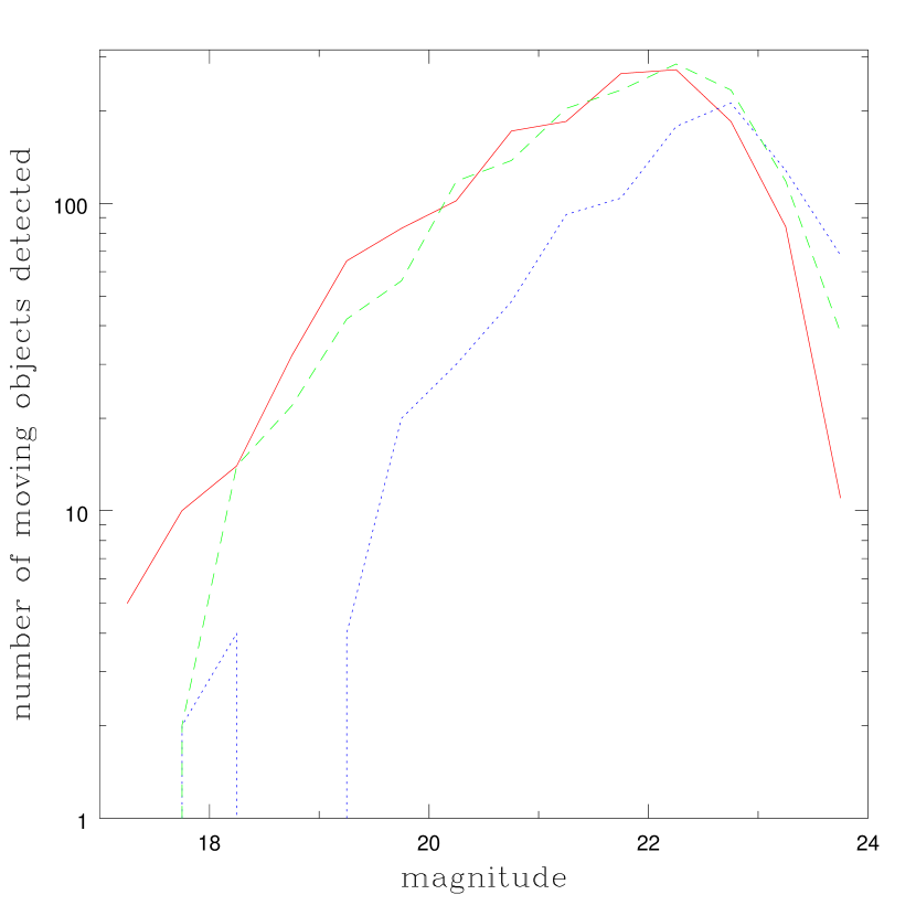
Figure 2.— Magnitude distribution of moving objects detected in the DLS. Detections in the $B$, $V$, and $R$ passbands are represented by dotted, dashed, and solid lines, respectively. Some objects were detected in more than one filter, but most were not.

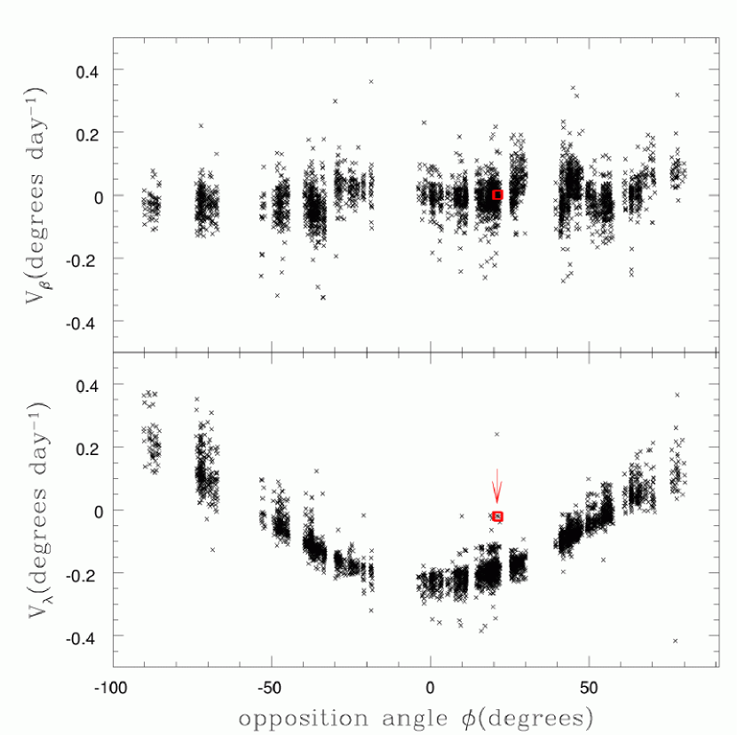
Figure 3.— The moving object velocity distributions in ecliptic coordinates. Two Kuiper Belt objects detailed in Section 5.1 are marked with a red box. They clearly stand out from the main belt $v_{\lambda}$ distribution, and neighboring points are also likely KBOs. Overall, KBOs do not stand out in the $v_{\beta}$ distribution.

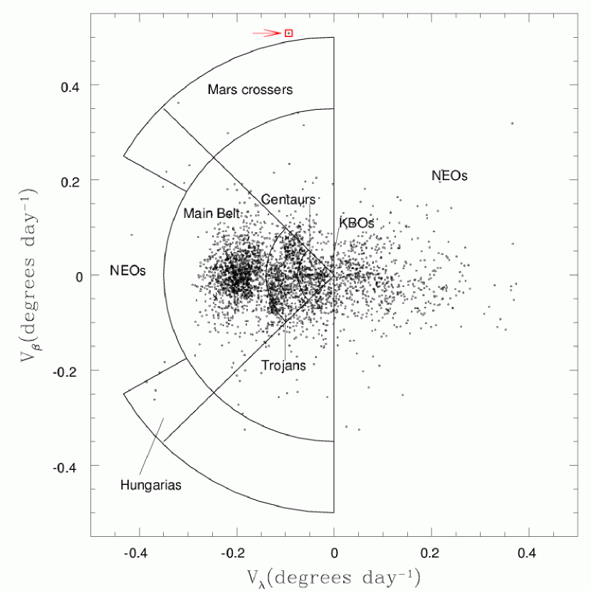
Figure 4.— Tentative classification of moving objects into asteroid families, based on velocities. The object boxed at top is the fast-moving object detailed in Section 5.2.

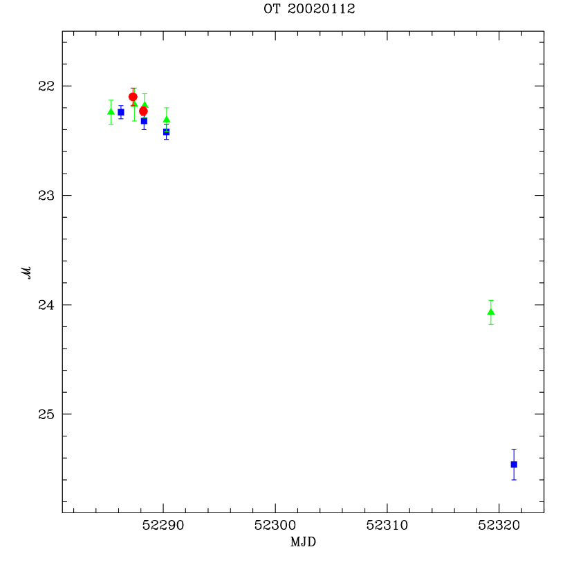
Figure 5.— Lightcurve OT 20020112 in differential flux magnitudes $\mathcal{M}$ in the $B$ (square datapoints), $V$ (triangle), and $R$ (circle) passbands. The data were obtained at the CTIO 4–m Blanco telescope and the KPNO 1.3m MDM telescope. All data from a given MJD are averaged together after being placed on similar magnitude systems during the difference imaging process. Lightcurve information is presented in Table 2. There is no apparent host for this variability in images obtained prior to and subsequent to the observed event.

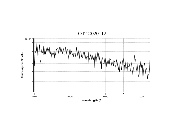
Figure 6.— Spectrum of OT 20020112 obtained 6 days after detection. The phase of the event is uncertain. Weak emission features indicate a possible redshift of $z=0.038$. However, we are unable to detect a host to $R>27.6$. This transient represents a class of objects that vary on timescales of tens of days, much like supernovae or potentially optical GRB orphans, but have no apparent host galaxy.

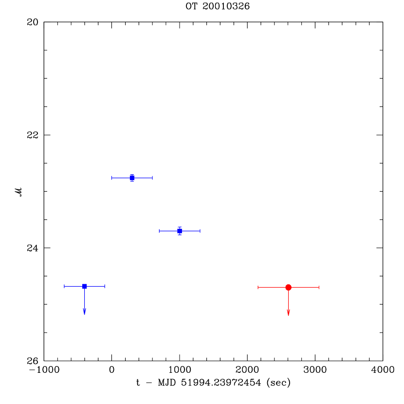
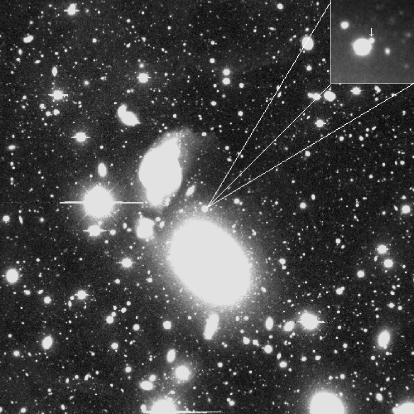
Figure 7.— $B$ and $R$–band lightcurve (square and circular symbols, respectively) in differential flux magnitudes $\mathcal{M}$ (see Equation 1), and $8.6\arcmin$ x $8.6\arcmin$ $R$–band template image, of OT 20010326. The latter shows its position in the field of Abell 1836, at $z=0.036$. The precursor is to the immediate north–west of the (saturated) brighter star, where north is up and east is to the left. Radio source and elliptical galaxy PKS 1358-11 is to the south, and spiral galaxy LCRS B135905.8-112006 is to the north–east.

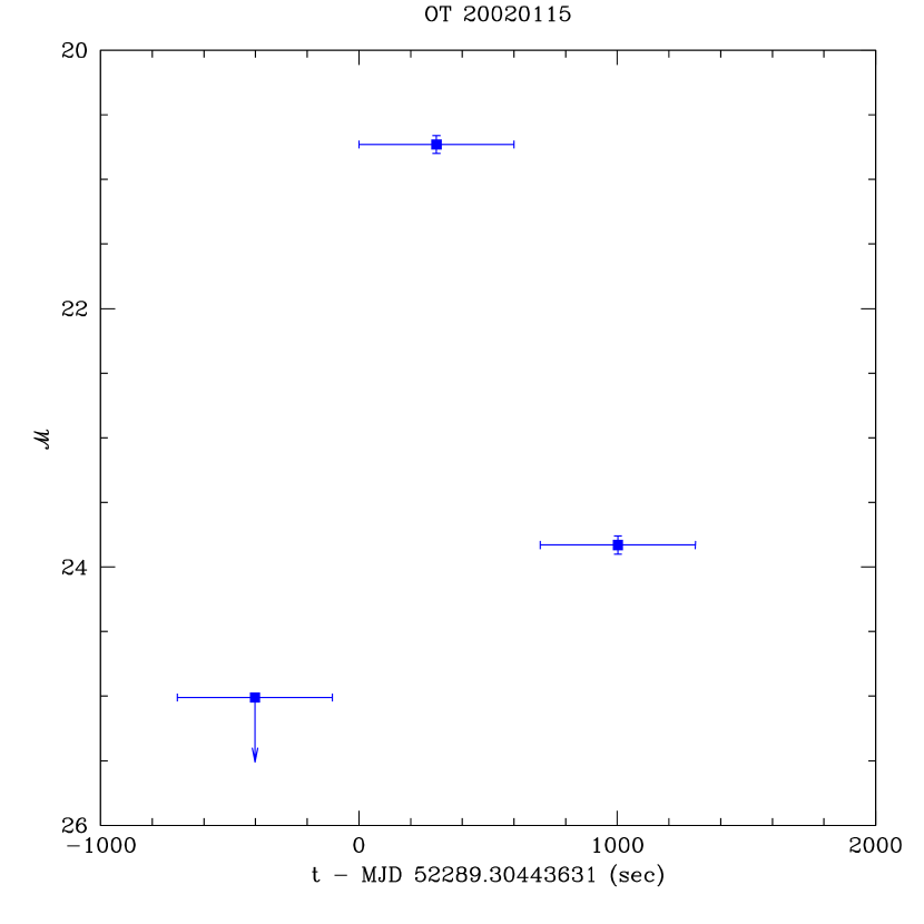
Figure 8.— $B$–band temporal lightcurve of OT 20020115 in differential flux magnitudes $\mathcal{M}$.

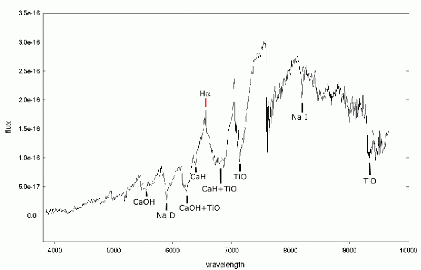
Figure 9.— Post–event spectrum of OT 20020115. The spectrum was obtained with the Magellan 1 telescope 3 days after the transient event depicted in Figure 8. The clear emission in H$\alpha$ and absorption by TiO bands indicates Galactic origin. Overall, the spectral features and composite colors are consistent with a late type (dM4) flare star.

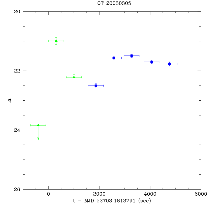
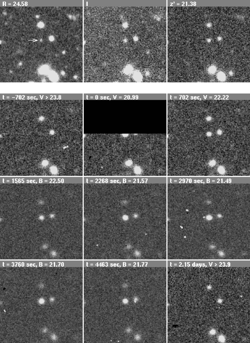
Figure 10.— Lightcurve of OT 20030305, in differential flux magnitudes $\mathcal{M}$, in the $B$ and $V$ passbands (square and triangular datapoints, respectively). The image sequence corresponding to these data points is shown in $40\arcsec$ x $40\arcsec$ panels to the right. The top 3 images show the host, or precursor, of the transient in $R$, $I$, and $z^{\prime}$ (we have no calibration data for the $I$–band image). The images below show the time evolution of the event, from the constraining image $700s$ before, to the first image 2 days after where it was undetected in $V$. The time of each observation relative to the detection of the event is indicated, as well as the measured brightness of the transient, where these numbers were derived from photometry on the difference images. Our first detection of this transient landed on the boundary of a MOSAIC chip, the dark region in the above detection image. In all images, north is up and east is to the left.

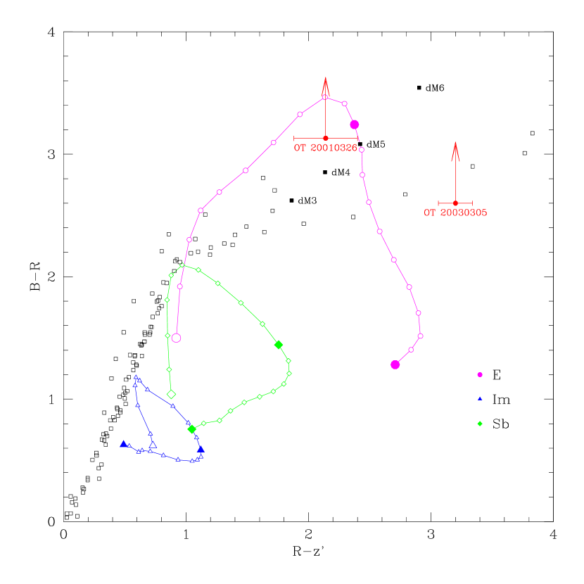
Figure 11.— $B-R$ vs. $R-z^{\prime}$ diagram for the precursor/host objects of OT 20010326 and OT 20030305. The open squares represent the Pickles (1998) stellar library of energy distributions, with solid squares indicating the approximate positions of dM3–6 dwarf stars. The tracks indicate K–corrected colors for elliptical (circle), irregular (triangle), and Sb (diamond) galaxies with increasing redshift (steps of $z=1$ are indicated by filled symbols, starting with the large open symbol at $z=0$) based on galaxy spectral templates from Coleman et al. (1980). These are shown to indicate regions where contamination of stellar precursor identifications by compact high redshift galaxies is expected.

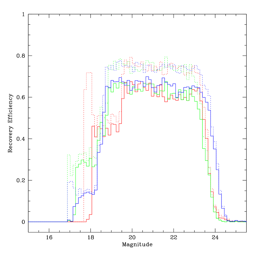
Figure 12.— Transient point–source detection efficiency as a function of magnitude in the difference image ($\mathcal{M}$), for the $B$, $V$, and $R$ passbands. The dotted histograms are our raw point source detection efficiencies, while the solid histograms represent our efficiencies after cuts. The bright end cutoff represents the level at which the objects become saturated, with additional efficiency coming from the recovery of the wings of the saturated object. In our efficiency analysis, we explicity set our efficiency for objects brighter than saturation ($\mathcal{M}_{B}\leq 18.6,\mathcal{M}_{V}\leq 18.8$ and $\mathcal{M}_{R}\leq 19.5$) equal to zero. The dim cutoff represents the 2.5 $\sigma$ detection limit of single images in our transient search.

Table 1Unusual Transient Event Summary

Event	DLS Subfield	RA (J2000)	DEC (J2000)	$B$	$V$	$R$	$z^{\prime}$
OT 20020112	F4p13	10:49:32.8	-04:31:45	$>27.3$	$>27.2$	$>27.7$	$>24.9$
$\cdots$				$>27.2$	$>27.0$	$>27.6$	$>24.8$
OT 20010326	F5p31	14:01:42.2	-11:35:15	$>26.4$	$24.48\pm 0.10$	$23.30\pm 0.12$	$21.16\pm 0.11$
$\cdots$				$>26.2$	$24.27\pm 0.10$	$23.13\pm 0.12$	$21.06\pm 0.11$
OT 20020115	F4p23	10:48:56.1	-05:00:41	$21.25\pm 0.07$	$19.67\pm 0.05$	$<19.5$	$16.28\pm 0.09$
OT 20030305	F4p31	10:53:45.8	-05:37:44	$>27.2$	$>27.1$	$24.58\pm 0.10$	$21.38\pm 0.13$
$\cdots$				$>27.0$	$>27.0$	$24.50\pm 0.10$	$21.34\pm 0.13$

Note. — Summary of selected optical transients (OTs) from the DLS transient survey. OT 20020112 varied on the timescale of months, and we fail to detect a host or precursor object to the reported limiting magnitudes. The other three events varied on thousand–second timescales, and were resolved in multiple survey images. Magnitudes are Vega–based and represent any detected precursor or host in its quiescent state. A second set of magnitudes takes into account Schlegel et al. (1998) corrections for Galactic reddening, assuming a $R_{V}=3.1$ extinction curve, except for OT 20020115 which is known to be Galactic in origin. Point source limits from Equation 2 are quoted for null detections.

Table 2Optical Transient Event Photometry

Event	MJD	Passband	$\mathcal{M}$	$\mathcal{M}_{C}$
OT 20020112	52285.3	V	$22.24\pm 0.11$	$22.11\pm 0.11$
	52286.2	B	$22.24\pm 0.06$	$22.07\pm 0.06$
	52287.2	R	$22.10\pm 0.08$	$22.00\pm 0.08$
	52287.4	V	$22.17\pm 0.15$	$22.04\pm 0.15$
	52288.2	R	$22.23\pm 0.04$	$22.13\pm 0.04$
	52288.2	B	$22.32\pm 0.08$	$22.15\pm 0.08$
	52288.3	V	$22.18\pm 0.11$	$22.05\pm 0.11$
	52290.2	B	$22.42\pm 0.07$	$22.25\pm 0.07$
	52290.3	V	$22.31\pm 0.11$	$22.18\pm 0.11$
	52319.2	V	$24.07\pm 0.11$	$23.94\pm 0.11$
	52321.3	B	$25.46\pm 0.14$	$25.29\pm 0.14$
OT 20010326	51994.2315949	B	$>24.8$	$>24.4$
	51994.2397245	B	$22.76\pm 0.06$	$22.50\pm 0.06$
	51994.2478576	B	$23.70\pm 0.07$	$23.44\pm 0.07$
	51994.2646898	R	$>24.7$	$>24.5$
OT 20020115	52289.2963074	B	$>25.0$	$\cdots$
	52289.3044363	B	$20.73\pm 0.07$	$\cdots$
	52289.3125651	B	$23.83\pm 0.07$	$\cdots$
	52290.2594999	B	$>24.8$	$\cdots$
OT 20030305	52703.1732501	V	$>23.8$	$>23.7$
	52703.1813791	V	$20.99\pm 0.12$	$20.89\pm 0.12$
	52703.1895094	V	$22.22\pm 0.09$	$22.12\pm 0.09$
	52703.1995017	B	$22.50\pm 0.08$	$22.37\pm 0.08$
	52703.2076305	B	$21.57\pm 0.06$	$21.44\pm 0.06$
	52703.2157589	B	$21.49\pm 0.06$	$21.36\pm 0.06$
	52703.2249089	B	$21.70\pm 0.06$	$21.57\pm 0.06$
	52703.2330383	B	$21.77\pm 0.07$	$21.64\pm 0.07$
	52705.3304513	V	$>23.9$	$>23.8$

Note. — Differential flux magnitudes $\mathcal{M}$ for each optical transient, in the Vega system. Also listed are the Modified Julian Day (MJD) and filter for each observation. OT 20020112 varied on a month-long timescale, and the photometry listed represents the MJD–averaged brightness. The constraining observations preceding and following the event are also listed for the short timescale transients. Limits on $\mathcal{M}$ are determined by adding input PSFs to the difference images. Error bars include systematic calibration errors added in quadrature with the experimental uncertainties in the measurement. $\mathcal{M}_{C}$ represents Schlegel et al. (1998) corrected magnitudes, assuming a source outside the Galactic extinction layer, except for OT 20020115 which is known to be Galactic in origin.

Table 3Event rate

Filter	Timescale	Exposure ${\it E}$ (deg2–days)	$\mathcal{M}_{min}$	$\mathcal{M}_{max}$	$\left<{\cal E}\right>$	$N_{obs}$	$N_{max,95\%}$	$\eta$	$\eta_{max,95\%}$
B	1300s	1.1	18.6	23.8	0.65	3	7.8	6.5	17
$\cdots$	$\cdots$	$\cdots$	$\cdots$	$\cdots$	$\cdots$	2	6.3	4.3	14
$\cdots$	$\cdots$	$\cdots$	$\cdots$	$\cdots$	$\cdots$	1	4.7	2.2	10
$\cdots$	$\cdots$	$\cdots$	$\cdots$	$\cdots$	$\cdots$	0	3.0	0.0	6.5
V	1300s	1.2	18.8	23.3	0.63	1	4.7	2.1	9.9
$\cdots$	$\cdots$	$\cdots$	$\cdots$	$\cdots$	$\cdots$	0	3.0	0.0	6.3
R	1900s	1.5	19.5	23.4	0.62	0	3.0	0.0	5.2
B+V+R	$\cdots$	3.7	$\cdots$	$\cdots$	0.63	4	9.2	2.7	6.3
$\cdots$	$\cdots$	$\cdots$	$\cdots$	$\cdots$	$\cdots$	3	7.8	2.0	5.3
$\cdots$	$\cdots$	$\cdots$	$\cdots$	$\cdots$	$\cdots$	2	6.3	1.4	4.3
$\cdots$	$\cdots$	$\cdots$	$\cdots$	$\cdots$	$\cdots$	1	4.7	0.7	3.2
$\cdots$	$\cdots$	$\cdots$	$\cdots$	$\cdots$	$\cdots$	0	3.0	0.0	2.0

Note. — For each filter, we present our sensitivity to transients for timescales at twice the typical exposure times plus $100s$ of camera readout. We list the magnitude ranges over which our efficiency of recovering a transient is approximated by a constant $\left<{\cal E}\right>$. Assuming we have detected $0\leq N\leq N_{obs}$ events per filter, we also list the maximum number of events allowed by Poisson statistics at the $95\%$ confidence level, for any model of temporal variability. We derive the corresponding event rate $\eta$ in events deg${}^{-2}~{}{\rm day}^{-1}$.

References

- Afonso et al. (2003) Afonso, C., et al. 2003, A&A, 400, 951
- Akerlof et al. (1993) Akerlof, C., et al. 1993, in BATSE Gamma Ray Burst Workshop, 21–23, 2
- Akerlof et al. (2003) Akerlof, C. W., et al. 2003, PASP, 115, 132
- Alard (2000) Alard, C. 2000, A&AS, 144, 363
- Alcock et al. (2000b) Alcock, C., et al. 2000b, ApJ, 542, 281
- Aldering et al. (2002) Aldering, G., Adam, G., Antilogus, P., Astier, P., Bacon, R., Bongard, S., Bonnaud, C., Copin, Y., Hardin, D., Henault, F., Howell, D. A., Lemonnier, J., Levy, J., Loken, S. C., Nugent, P. E., Pain, R., Pecontal, A., Pecontal, E., Perlmutter, S., Quimby, R. M., Schahmaneche, K., Smadja, G., & Wood-Vasey, W. M. 2002, in Survey and Other Telescope Technologies and Discoveries. Edited by Tyson, J. Anthony; Wolff, Sidney. Proceedings of the SPIE, Volume 4836, pp. 61-72 (2002)., 61–72
- Alves et al. (2003) Alves, D. R., et al. 2003, in IAU Symposium 220
- Barris et al. (2003) Barris, B., et al. 2003, Submitted
- Becker (2003a) Becker, A. 2003a, IAU Circ., 8093, 2
- Becker (2003b) —. 2003b, IAU Circ., 8094, 2
- Becker et al. (2002a) Becker, A., et al. 2002a, IAU Circ., 7833, 1
- Becker et al. (2003) Becker, A., Loomba, D., & Wilcox, R. 2003, IAU Circ., 8093, 1
- Becker et al. (2002b) Becker, A., et al. 2002b, IAU Circ., 7803, 2
- Becker et al. (2002c) Becker, A., et al. 2002c, IAU Circ., 7804, 1
- Becker et al. (2002d) Becker, A. C., et al. 2002d, GRB Circular Network, 1217, 1
- Berger et al. (2003) Berger, E., et al. 2003, ApJ, 588, 99
- Bernstein & Khushalani (2000) Bernstein, G. & Khushalani, B. 2000, AJ, 120, 3323
- Bernstein & Jarvis (2002) Bernstein, G. M. & Jarvis, M. 2002, AJ, 123, 583
- Bertin & Arnouts (1996) Bertin, E. & Arnouts, S. 1996, A&AS, 117, 393
- Bloom et al. (2003) Bloom, J. S., et al. 2003, ApJ, 599, 957
- Boeshaar et al. (2003) Boeshaar, P. C., Margoniner, V., & The Deep Lens Survey Team. 2003, in IAU Symposium 211, E. Martin, ed., Astron. Soc. Pacific. 203
- Clocchiatti et al. (2002) Clocchiatti, A., et al. 2002, GRB Circular Network, 1218, 1
- Coleman et al. (1980) Coleman, G. D., Wu, C.-C., & Weedman, D. W. 1980, ApJS, 43, 393
- Condon et al. (1998) Condon, J. J., et al. 1998, AJ, 115, 1693
- Dermer et al. (1999) Dermer, C. D., Chiang, J., & Böttcher, M. 1999, ApJ, 513, 656
- Filippenko et al. (2001) Filippenko, A. V., et al. 2001, in ASP Conf. Ser. 246: IAU Colloq. 183: Small Telescope Astronomy on Global Scales, 121–+
- Fresneau et al. (2001) Fresneau, A., et al. 2001, AJ, 121, 517
- Gal-Yam et al. (2002) Gal-Yam, A., et al. 2002, PASP, 114, 587
- Granot et al. (2000) Granot, J., Piran, T., & Sari, R. 2000, ApJ, 534, L163
- Griffith & Wright (1993) Griffith, M. R. & Wright, A. E. 1993, AJ, 105, 1666
- Groot et al. (2003) Groot, P. J., et al. 2003, MNRAS, 339, 427
- Gurzadian (1980) Gurzadian, G. A. 1980, Oxford Pergamon Press International Series on Natural Philosophy, 101
- Howell et al. (1996) Howell, S. B., et al. 1996, AJ, 112, 1302
- Huang et al. (2002) Huang, Y. F., Dai, Z. G., & Lu, T. 2002, MNRAS, 332, 735
- Ivezić et al. (2003) Ivezić, Ž., et al. 2003, Memorie della Societa Astronomica Italiana, 74, 978
- Ivezić et al. (2001) Ivezić, Ž., et al. 2001, AJ, 122, 2749
- Jannuzi & Dey (1999) Jannuzi, B. T. & Dey, A. 1999, in ASP Conf. Ser. 191: Photometric Redshifts and the Detection of High Redshift Galaxies, 111–+
- Kaiser et al. (2002) Kaiser, N., et al. 2002, in Survey and Other Telescope Technologies and Discoveries. Edited by Tyson, J. Anthony; Wolff, Sidney. Proceedings of the SPIE, Volume 4836, pp. 154-164 (2002)., 154–164
- Kirkman et al. (2000) Kirkman, D., et al. 2000, IAU Circ., 7398, 2
- Knop et al. (2003) Knop, R. A., et al. 2003, ApJ, 598, 102
- Kunkel (1973) Kunkel, W. E. 1973, ApJS, 25, 1
- Kunkel (1975) Kunkel, W. E. 1975, in IAU Symp. 67: Variable Stars and Stellar Evolution, 15–46
- Landolt (1992) Landolt, A. U. 1992, AJ, 104, 340
- Le Floc’h et al. (2003) Le Floc’h, E., et al. 2003, A&A, 400, 499
- Li & Paczyński (1998) Li, L. & Paczyński, B. 1998, ApJ, 507, L59
- Li et al. (2003) Li, W., et al. 2003, ApJ, 586, L9
- Mahabal et al. (2003) Mahabal, A., et al. 2003, American Astronomical Society Meeting, 203,
- Malkan et al. (1998) Malkan, M. A., Gorjian, V., & Tam, R. 1998, ApJS, 117, 25
- Millis et al. (2002) Millis, R. L., et al. 2002, AJ, 123, 2083
- Monet et al. (1998) Monet, D. B. A., et al. 1998, VizieR Online Data Catalog, 1252, 0
- Nakar et al. (2002) Nakar, E., Piran, T., & Granot, J. 2002, ApJ, 579, 699
- Nemiroff (2003) Nemiroff, R. J. 2003, AJ, 125, 2740
- Paulin-Henriksson et al. (2003) Paulin-Henriksson, S., et al. 2003, A&A, 405, 15
- Perkins et al. (2000) Perkins, S., et al. 2000, in Proceedings of SPIE, Vol. 4120, 52–62
- Pickles (1998) Pickles, A. J. 1998, PASP, 110, 863
- Pojmański (2001) Pojmański, G. 2001, in ASP Conf. Ser. 246: IAU Colloq. 183: Small Telescope Astronomy on Global Scales, 53–+
- Pravdo et al. (1999) Pravdo, S. H., et al. 1999, AJ, 117, 1616
- Reid et al. (1995) Reid, I. N., Hawley, S. L., & Gizis, J. E. 1995, AJ, 110, 1838
- Rest et al. (2004) Rest, A., et al. 2004, In preparation
- Rhoads (1997) Rhoads, J. E. 1997, ApJ, 487, L1+
- Rhoads (2003) —. 2003, ApJ, 591, 1097
- Rose et al. (1995) Rose, J., et al. 1995, in ASP Conf. Ser. 77: Astronomical Data Analysis Software and Systems IV, 429–+
- Sari et al. (1998) Sari, R., Piran, T., & Narayan, R. 1998, ApJ, 497, L17+
- Schlegel et al. (1998) Schlegel, D. J., Finkbeiner, D. P., & Davis, M. 1998, ApJ, 500, 525+
- Smail et al. (2002) Smail, I., et al. 2002, ApJ, 581, 844
- Smith et al. (2002a) Smith, J. A., et al. 2002a, AJ, 123, 2121
- Smith et al. (2002b) Smith, R. C., et al. 2002b, American Astronomical Society Meeting, 201, 0
- Spergel et al. (2003) Spergel, D. N., et al. 2003, ApJS, 148, 175
- Stokes et al. (2000) Stokes, G. H., et al. 2000, Icarus, 148, 21
- Sumi et al. (2003) Sumi, T., et al. 2003, ApJ, 591, 204
- Tonry et al. (2003) Tonry, J. L., et al. 2003, ApJ, 594, 1
- Tyson (2002) Tyson, J. A. 2002, in Survey and Other Telescope Technologies and Discoveries. Edited by Tyson, J. Anthony; Wolff, Sidney. Proceedings of the SPIE, Volume 4836, pp. 10-20 (2002)., 10–20
- Van Den Bergh (2003) Van Den Bergh, S. 2003, ApJ, 590, 797
- Vanden Berk et al. (2002) Vanden Berk, D. E., et al. 2002, ApJ, 576, 673
- Vestrand et al. (2002) Vestrand, W. T., et al. 2002, in Advanced Global Communications Technologies for Astronomy II. Edited by Kibrick, Robert I. Proceedings of the SPIE, Volume 4845, pp. 126-136 (2002)., 126–136
- Vivas et al. (2001) Vivas, A. K., et al. 2001, ApJ, 554, L33
- Voges et al. (2000) Voges, W., et al. 2000, VizieR Online Data Catalog, 9029, 0
- White et al. (1997) White, R. L., et al. 1997, ApJ, 475, 479
- Wittman et al. (2000) Wittman, D. M., et al. 2000, IAU Circ., 7551, 1
- Wittman et al. (2002) Wittman, D. M., et al. 2002, in Survey and Other Telescope Technologies and Discoveries. Edited by Tyson, J. Anthony; Wolff, Sidney. Proceedings of the SPIE, Volume 4836, pp. 73-82 (2002)., 73–82
- Wozniak et al. (2001) Wozniak, P. R., et al. 2001, Acta Astronomica, 51, 175
- Wozniak et al. (2004) Wozniak, P. R., et al. 2004, AJin press, astro-ph/0401217