CENTRAL STARS OF PLANETARY NEBULAE IN THE LARGE MAGELLANIC CLOUD: A FAR-UV SPECTROSCOPIC ANALYSIS

Abstract

We observed seven central stars of planetary nebulae (CSPN) in the Large Magellanic Cloud (LMC) with the Far Ultraviolet Spectroscopic Explorer (FUSE), and performed a model-based analysis of these spectra in conjunction with Hubble Space Telescope (HST) spectra in the UV and optical range to determine the stellar and nebular parameters. Most of the objects show wind features, and they have effective temperatures ranging from 38 to 60 kK with mass-loss rates of $\simeq 5\mbox{\,$\rm x10^{-8}$}$  $\rm{M_{\odot}\>yr^{-1}}$. Five of the objects have typical LMC abundances. One object (SMP LMC 61) is a [WC4] star, and we fit its spectra with He/C/O-rich abundances typical of the [WC] class, and find its atmosphere to be iron-deficient. Most objects have very hot ($T\gtrsim 2000$ K) molecular hydrogen (H₂) in their nebulae, which may indicate a shocked environment. One of these (SMP LMC 62) also displays O VI 1032-38 nebular emission lines, rarely observed in PN.

1 INTRODUCTION

With respect to the study of planetary nebulae (PN) systems, those in the Large Magellanic Cloud (LMC) are important for two primary reasons. Attempts to describe the evolution of Galactic PN are hindered by large relative uncertainties in their distances, which carry over into physical parameters such as the stellar luminosity and radius of the central star of the PN (CSPN), and the size and ionized mass of the PN itself. This obstruction is removed for the PN of the LMC, all of which lie at essentially at the same distance, allowing the physical parameters to be scaled to absolute values. Additionally, the lower metallicity of the LMC relative to the Milky Way allows the role of metallicity in low/intermediate-mass stellar evolution to be assessed. The largest impact a higher metallicity is expected to have on a star’s evolution is a more efficient radiative driving during its windy phases: the asymptotic giant branch (AGB) phase, the post-AGB phase, and/or perhaps a Wolf-Rayet phase [WR]. This would increase the star’s mass-loss rate, and thus slow its evolution during these periods. Such an effect would manifest itself in the form of different relative population ratios in galaxies of varying metallicities. These implications carry over into galaxy evolution, through chemical evolution and the dynamic interactions between the star’s ejected material and the surrounding interstellar medium (ISM). Although these effects are not as dramatic on an individual basis as those of a massive star, the large fraction of stars that evolve through the CSPN phase make their contribution to the Galactic chemical evolution significant (see, e.g., Marigo, 2001 for a discussion).

Characterization of an individual PN system requires an understanding of both the PN and its central star. Several non-LTE (NLTE) spectroscopic studies of Galactic CSPN in the optical range have been carried out, both of CSPN without winds using plane-parallel analyses (e.g., Mèndez et al., 1985; Herrero et al., 1990) and of CSPN with winds using spherical codes (e.g., Leuenhagen & Hamann, 1998; Koesterke & Hamann, 1997; De Marco & Crowther, 1998). The sample of known LMC PN for which HST spectroscopy exists includes only the brightest and rather compact objects. The nebular continuum of compact (high density) PN typically masks the light of the central star for wavelengths longwards of $\sim$1215 Å (Bianchi et al., 1997), complicating the task of characterizing the two components if relying solely on UV and optical data. Characteristics of a large sample of LMC CSPN have been inferred from photoionization models of their nebular spectra (e.g., Dopita & Meatheringham, 1991a; Vassiliadis et al., 1996, 1998a). A handful have been analyzed using nebular continuum models in conjunction with modeling of the central star in the UV (e.g., Bianchi et al., 1997; Dopita et al., 1997). With the Far-Ultraviolet Spectroscopic Explorer (FUSE) , it is now possible to observe LMC CSPN at far-UV wavelengths where the spectrum is unaffected by nebular contamination. Far-UV/UV analyses of Galactic CSPN with winds have been carried out by Koesterke & Werner (1998) and Herald & Bianchi (2004a). The far-UV is where these hot stars emit most of their observable flux and often exhibit their strongest photospheric and/or wind features. Herald & Bianchi (2004b) performed an analysis of the far-UV spectra of the Galactic CSPN K1-26, and derived a significantly higher temperature (120 vs. 65 kK) than had resulted from analysis of optical spectra (Mèndez et al., 1985), illustrating the value of far-UV-based analyses.

Motivated by the above considerations, we observed a sample of seven CSPN with FUSE as part of Bianchi’s cycle 2 program B001. The FUSE spectra allow us to separate the nebular and central star components and to characterize the physical parameters of each through modeling. The FUSE range also includes strong absorption due to molecular hydrogen (H₂), which is also modeled concurrently.

This paper is arranged as follows. The observations and data reduction are described in § 2. A comparison of the spectra of the objects is presented in § 3. Our models and parameter determinations are described in § 4. The implications of our results are discussed in § 5 and our conclusions in § 6.

2 OBSERVATIONS AND REDUCTION

For our analysis, we used far-UV data taken with the Far Ultraviolet Spectroscopic Explorer (FUSE) and archive UV data gathered with the Hubble Space Telescope’s (HST) Faint Object Spectrograph (FOS) or Space Telescope Imaging Spectrograph (STIS).

2.1 Far-UV Data

The FUSE observations of our sample stars are summarized in Table 1. They represent some of the dimmest stellar objects yet observed by FUSE, and necessitated long integration times.

FUSE covers the wavelength range 905—1187 Å at a spectral resolution of $R\approx 20,000$ ($\sim$ 15  $\rm{km\>s^{-1}}$). It is described by Moos et al. (2000) and its on-orbit performance is discussed by Sahnow et al. (2000). FUSE collects light concurrently in four different channels (LiF1, LiF2, SiC1, and SiC2), each of which is divided into two segments (A & B) recorded by two detectors, covering different subsets of the above range with some overlap. We used FUSE’s LWRS (30″$\times$30″) aperture. These data, taken in “time-tag” mode, have been calibrated using the most recent FUSE data reduction pipeline, efficiency curves and wavelength solutions (CALFUSE v2.2.2).

Because of their faintness, most of our targets required many orbit-long exposures, each of which typically had low count-rates and thus signal-to-noise ratios. Each calibrated extracted sequence was checked for unacceptable count-rate variations (a sign of detector drift), incorrect extraction windows, and other anomalies. Segments with problems were not included in further steps. The 2-D spectra were checked to ensure no secondary objects contaminated the exposure.

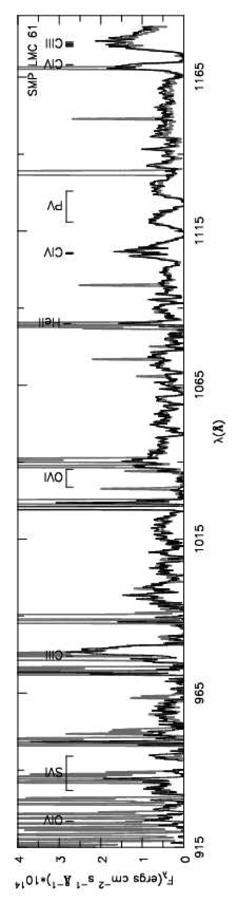
Figure 1: SMP LMC 61 observations: Comparison of the “night only” data (black line) with the combined day and night (“all”) data (gray line). Strong terrestrial airglow lines (e.g. O I) are seen in many regions of interest in the pipeline extraction of combined data. Due to the orientation of FUSE, scattered solar lines (e.g. O VI) appear in the SiC detectors. The data are convolved with a 0.25 Å Gaussian for clarity.

An example of FUSE observations is shown in Fig. 1. Two data reductions are shown for one object: all the “good” data (i.e., not affected by bursts or other anomalies), and only the good data taken during the night portion of the orbits (when the spacecraft was on the dark side of the Earth). The spectrum is contaminated by both strong terrestrial airglow lines (such as O I and N I), and scattered solar features (O VI in this case, and C IIIin others). The latter appear in the SiC detectors due to the orientation of FUSE. Because the terrestrial/solar features often confuse the CSPN observations, we only used the night-only data in our spectral analysis, and all FUSE spectra henceforth presented in this paper will be night-only. Note that some residual airglow lines (usually O I) still sometimes appear in this night only data.

All the “good” calibrated exposures were combined using FUSE pipeline routines. The default FUSE pipeline attempts to model the background measured off-target and subtracts it from the target spectrum. We found that, for our fainter objects, the background appeared to be over-estimated with this method, particularly at shorter wavelengths (i.e., $<1000$ Å). We therefore tried two other reductions. In the first, subtraction of the measured background is turned off and the background is taken to be the model scattered-light scaled by the exposure time. In the second, the first few steps of the pipeline are run on the individual exposures (which correct for effects unique to each exposure such as Doppler shift, grating motions, etc). The photon lists for the individual exposures are then combined and the remaining steps of the pipeline run on the combined file, with the motivation being that more total counts for both the target and background allow for a better extraction. However, this method did not result in a significant improvement over the others. The adopted background model for each star is indicated in Table 1.

The resulting calibrated data of the different channels were then compared for consistency. There are several regions of overlap between the different channels, and these were used to ensure that the continuum matched. For the fainter targets, often the continuum levels for different detectors did not agree. The procedure we typically adopted was to trust the LiF1a absolute flux calibration (which is most reliable — Sahnow et al., 2000), and scale the flux of the other detectors if needed. The LiF1b segment is severely affected by an artifact known as “the worm” (FUSE Data Handbook v1.3) and was not used, except in one case where it was in good agreement with the LiF2a. The SiC1 detector seemed frequently off-target, and other segments offered higher S/N data in the same range, so its data was often not used. In the end, we typically used the SiC2 data for wavelengths below $\sim 1000$ Å. Longwards of 1080 Å LiF2a data was employed. For the intermediate region (i.e., 1000–1080 Å), data from LiF1b, LiF2b, or both were used (data from one segment was omitted if it was discrepant with that of the SiC detectors). The region between 1083 and 1087 Å is not covered by the LiF detectors, and as the SiC detectors in this range were off-target, we have omitted this region (appearing as gaps in the observed data). Table 1 shows which segments and portions were used for the combined spectrum.

The results from the three different reduction methods were compared during the above process to understand if some features were actually artifacts of the background subtraction process. Data from near the detector edges were also omitted if they looked inconsistent.

The FUSE spectra presented in this paper were obtained by combining the good data from different segments, weighted by detector sensitivity, and rebinning to a uniform dispersion of 0.05 Å.

2.2 UV Data

Archival data from the HST’s Faint Object Spectrograph (FOS) and Space Telescope Imaging Spectrograph (STIS) instruments were also used longwards of 1200 Å, as summarized in Table 2. The FOS archive data were taken in the 1″ aperture, whose actual diameter following the COSTAR installation is 0.86″. The angular sizes of the LMC PN are typically $\lesssim$1″, so the FOS spectroscopy typically includes the entire nebula (the exception is SMP LMC 35 see Table CENTRAL STARS OF PLANETARY NEBULAE IN THE LARGE MAGELLANIC CLOUD: A FAR-UV SPECTROSCOPIC ANALYSIS). The utilized FOS dispersers include the G130H ($\mbox{\,$\Delta\lambda$}\sim 1$ Å), the G190H ($\mbox{\,$\Delta\lambda$}\sim 1.5$ Å), the G270H ($\mbox{\,$\Delta\lambda$}\sim 2$Å̃) and the G400H ($\mbox{\,$\Delta\lambda$}\sim 3$ Å). For SMP LMC 61, high-resolution STIS data was available, taken through the 52″x0.2″ aperture with the G140L ($\mbox{\,$\Delta\lambda$}\sim 1.3$ Å), G230L ($\mbox{\,$\Delta\lambda$}\sim 1.5$ Å) and G430L ($\mbox{\,$\Delta\lambda$}\sim 1.6$ Å) gratings.

Generally, the flux levels of the FUSE and FOS/STIS data in the region of overlap are in good agreement. However, for SMP LMC 2, the FOS flux levels were about 60 % those of FUSE. There was nothing in the FOS log files that suggested the observation may have been slightly off-target. We looked at the FUSE visitation images of the field during, and there is a UV-bright source that could have been within the FUSE aperture during the observation. Since FUSE has no spatial resolution, this source could have contaminated the observation. We assume this is the source of the discrepancy, and thus use the FOS flux level when scaling our parameters in the later analysis.

3 Description of Spectra

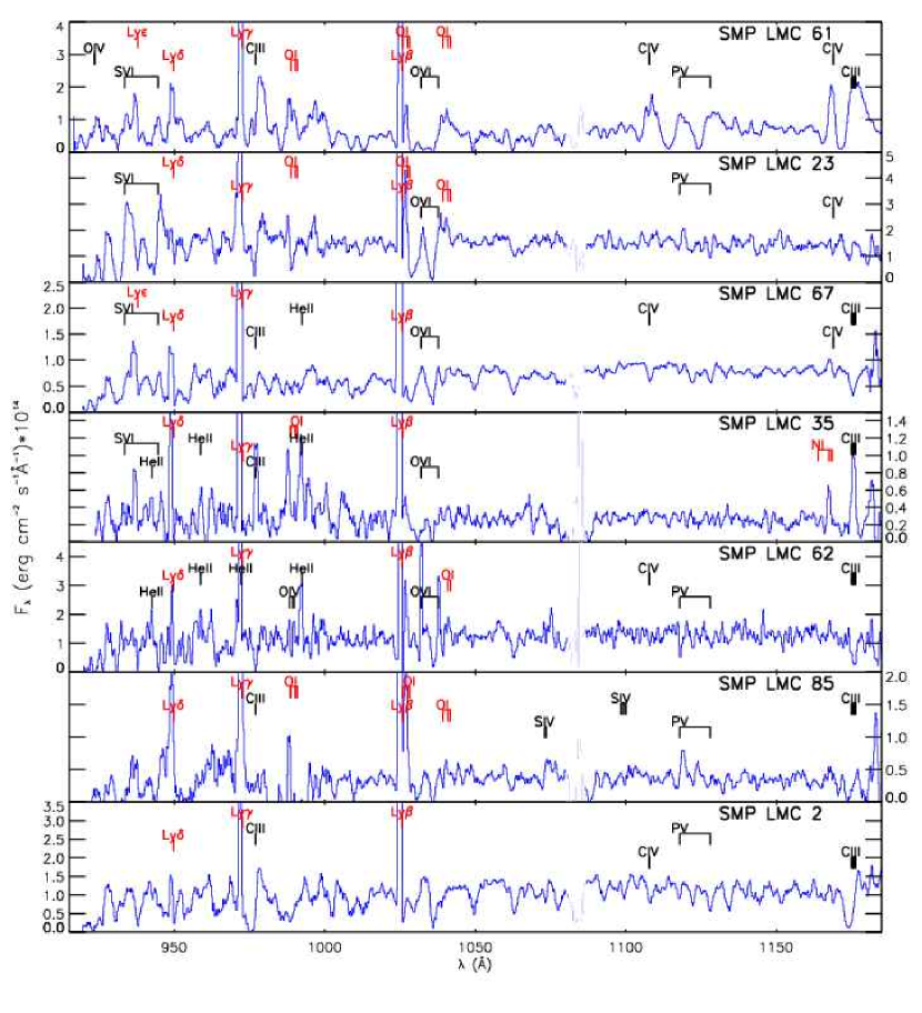
Figure 2: FUSE spectra of our sample, velocity shifted to the rest frame of the central star (Table 9), and rebinned to a resolution of 0.25Å. The more prominent stellar features and nebular emission lines are marked by black labels, airglow features are marked by the red/gray labels. Most objects display wind lines to some extent. C III features (either in absorption or P-Cygni) appear in most. The O VI doublet seems to be present in all cases except for SMP LMC 2, 62, and 85, where it is not obvious. Note the O VI $\lambda\lambda$1032-38 nebular emission features of SMP LMC 62, probably originating from shocks.

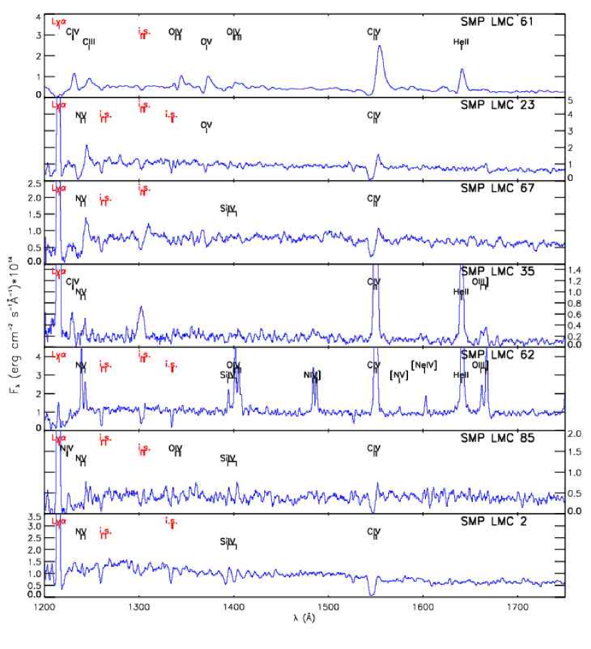
Figure 3: UV spectra (FOS and STIS) of our sample, velocity shifted to the rest frame of the central star (Table 9). The more prominent stellar features and nebular emission lines are marked with black labels, airglow lines or interstellar absorption features are marked with red/gray labels. Most objects display wind lines to some extent. C IV $\lambda\lambda$1548-51 appears as a P-Cygni profile in most. SMP LMC 62 shows a rich emission line spectrum typical of a shocked region.

The reduced FUSE spectra for the entire sample, along with line identifications, are shown in Fig. 2, and the UV spectra are shown in Fig.3. In Table 3, we list lines common in our sample, and classify them based on whether they appear as P-Cygni profiles, absorption lines, or nebular emission features. If a line appears as a strong P-Cygni profile and the blue edge of the absorption trough was not obviously obscured by other features (airglow lines or strong interstellar absorption features), we measured the terminal velocity based on its blue edge. This measurement,  v_edge, gives a fairly good indication of the wind terminal velocity,  v_∞, the difference between the two being the turbulent Doppler broadening, which is typically $\sim$10-20 %.

For most of the sample stars with wind signatures, $700\lesssim\mbox{\,v${}_{edge}$}\lesssim 1300$  $\rm{km\>s^{-1}}$. In the far-UV especially, H₂ absorption makes the continuum level very difficult to set (§ 4.1). Thus some measurements are more reliable than others. We used these measurements to initially estimate  v_∞ for our models (§ 4.3.5).

Five out of seven objects of our sample display definite wind signatures. SMP LMC 62 has questionable O VI wind features, and its UV lines are contaminated by nebular emission features. The FUSE spectra of SMP LMC 35, the dimmest object, has the lowest S/N and is not of sufficient quality to make a definitive statement about the existence of a wind. In its UV spectrum, nebular emission features again hide any present stellar features. There is a feature at $\sim 1300$ Å that could be a C III P-Cygni line, the strong O I interstellar absorption feature at 1300 Å is confusing the issue. We now discuss the individual spectra.

The UV spectra of SMP LMC 23 and LMC 67 are almost identical, both showing prominent wind lines of N V $\lambda\lambda$1238-43 and C IV $\lambda\lambda$1548-51. The blue edge of the C IV doublet indicates similar terminal velocities ($\simeq 1100$  $\rm{km\>s^{-1}}$) The far-UV spectra are likewise similar, with the wind lines (S VI $\lambda\lambda$933-44, C III $\lambda$977, O VI $\lambda\lambda$1032-38) of SMP LMC 23 being slightly stronger. A noticeable difference is C III $\lambda$1175, which is in absorption in SMP LMC 67 and filled in in SMP LMC 23.

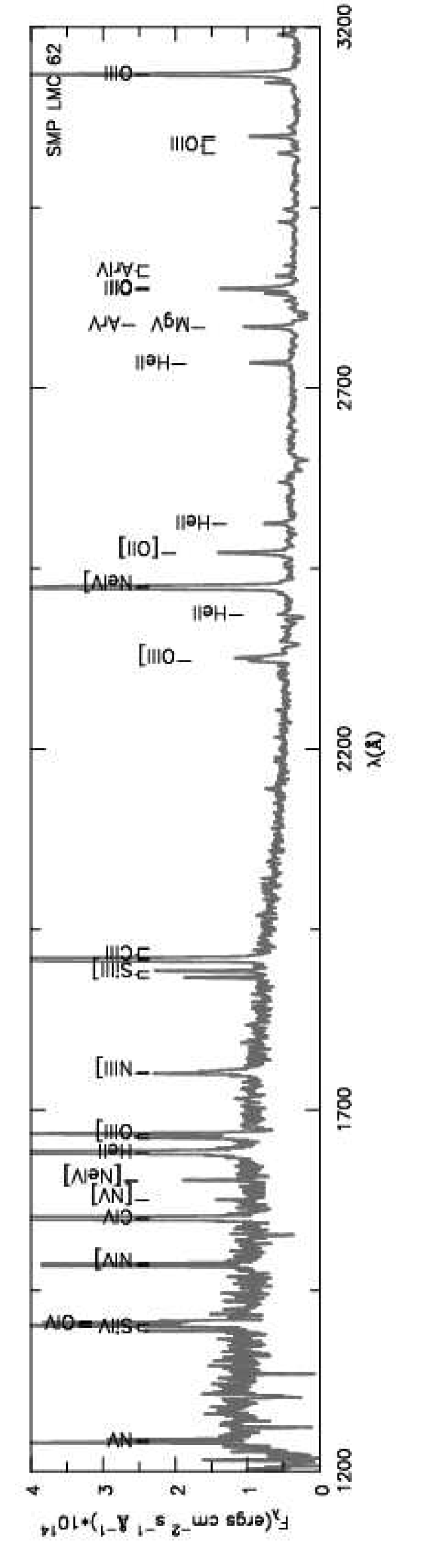
Figure 4: SMP LMC 62: The far-UV/UV spectrum of this object displays many highly-ionized emission lines characteristic of a shocked environment, such as N V $\lambda\lambda$1238-43 and [Ne V] $\lambda$1146.

Fig. 4 shows its far-UV and near-UV spectrum of SMP LMC 62. This star is unique among our sample, showing O VI $\lambda\lambda$1032-38 nebular features in its far-UV spectrum, as well as many high-ionization emission lines in its UV spectrum (such as [Ne V]). Table 4 lists the measured emission line fluxes for this object, determined by trapezoidal integration with suitable continuum subtraction.

The far-UV spectra of SMP LMC 62 is similar to that of SMP LMC 67, both showing weak (if any) S VI $\lambda\lambda$933-44, C III $\lambda$977 and O VI $\lambda\lambda$1032-38. C III $\lambda$1175 appears in absorption in both. One key difference is that SMP LMC 62 displays what appear to be nebular O VI emission features, which are unique in our sample. Such features have also been observed in the FUSE spectrum of the Galactic CSPN NGC 2371 (Herald & Bianchi, 2004a). The UV emission features mask C IV $\lambda\lambda$1548-51 if present. N V $\lambda\lambda$1238-43 may be a wind profile, but the nebular emission again confuses the issue.

SMP LMC 61 is a [WC] star, displaying a rich spectrum of Carbon and Oxygen P-Cygni features. There are no obvious nitrogen lines in its spectrum. SMP LMC 2 and SMP LMC 85 display C III in their far-UV spectra and have similar UV spectra, with the N V, Si IV, and C IV features of SMP LMC 85 being more prominent.

4 MODELING

Modeling the central stars of compact planetary nebulae presents some challenges. First, their optical spectra (and frequently their UV spectra also) are contaminated by the nebular continuum and lines, which obscure and sometimes entirely mask the stellar spectrum in these regions. Thus, one must rely on a smaller set of stellar features in the far-UV and UV to determine the stellar parameters. Second, the far-UV region, while not affected by nebular continuum emission, is affected by absorption by electronic transitions of sight-line molecular hydrogen (H₂). In our objects, such absorptions affect the entire far-UV region. Thus the analysis of these spectra consists of modeling the central star spectrum, the nebular continuum emission longwards of 1200 Å, and the sight-line Hydrogen (atomic and molecular) shortwards concurrently and to find a consistent solution. However, we discuss each in turn for clarity.

Throughout this paper, we adopt a LMC distance of $D=50.6$ kpc (Feast, 1991), and an LMC metallicity of $z=0.4\mbox{\,$\rm{Z_{\odot}}$}$ (Dufour, 1984) with values of “solar” abundances from Gray (1992).

4.1 Molecular and Atomic Hydrogen

Absorption due to atomic (H I) and molecular hydrogen (H₂) along the sight-line complicates the far-UV spectra of these objects. Toward a CSPN, this sight-line material typically consists of interstellar and circumstellar components. Material comprising the circumstellar H I and H₂ presumably was ejected from the star earlier in its history, and is thus important from an evolutionary perspective.

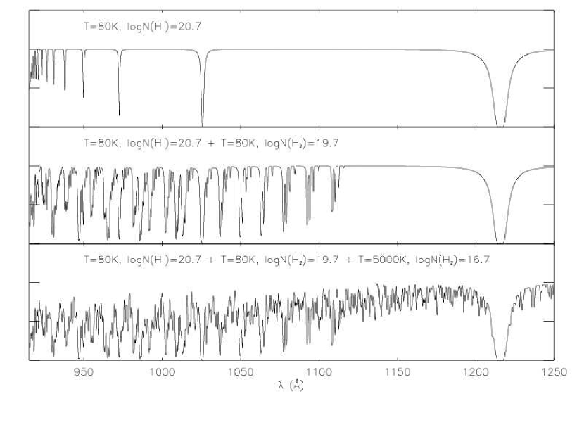
Figure 5: H₂ effects: The top plot shows a flat continuum to which are applied the absorption effects of an atomic hydrogen gas with characteristics of the ISM along a sight-line of low reddening [i.e., $T=80$ K, column density of $\mbox{\,$\log{N}$}(\mbox{\rm{{H~{}I}}})=20.7$ cm^-2], typical for our targets. The middle plot shows the absorption pattern of a typical low-reddening ( $E_{\rm{B-V}}$=0.1) interstellar H₂ gas [$T=80$, $\mbox{\,$\log{N}$}(\mbox{\rm{H}${}_{2}$})=19.7$ cm^-2], added to the previous. The bottom plot shows the effects of a relatively small quantity [$\mbox{\,$\log{N}$}(\mbox{\rm{H}${}_{2}$}^{hot})=16.7$ cm^-2] of hot ($T=5000$ K) H₂, similar to what we observe toward many of our LMC CSPN, applied to the previous. The entire FUSE range is affected by the dense field of transitions of numerous ro-vibrational H₂ states, which suppress the far-UV continuum.

The H₂ transitions in the FUSE range are from the Lyman ($B^{1}\Sigma^{+}_{u}$–$X^{1}\Sigma^{+}_{g}$) and Werner ($C^{1}\Pi^{\pm}_{u}$–$X^{1}\Sigma^{+}_{g}$) series. For a “cool” molecular gas (i.e., $\lesssim 100$ K) as found in the ISM, only the ground vibrational state is populated and the absorptions associated with its different rotational states show up as a series of discrete absorption “bands”, confined shortwards of $\lesssim 1115$ Å for typical IS column densities (i.e., $10^{18}$—$10^{19}$cm^-2) (see Fig. 5). The effects of such a gas are not difficult to correct for, because one can identify and use the unaffected parts of the stellar spectrum as a reference. However, we find that for many objects of our sample, a significant amount of hot (i.e., $T\gtrsim 1000$ K) H₂ lies along their sight-lines, presumably associated with the nebula. At such temperatures, higher vibrational states become populated and the absorption pattern is much more complex (again, see Fig. 5), obscuring the entire far-UV continuum spectrum. With care, the effects of such a gas can be accounted for and stronger stellar features can be discerned, but weaker stellar features will be unrecoverable.

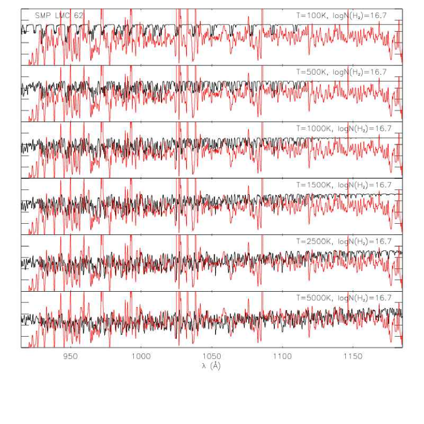
Figure 6: SMP LMC 62: Fitting hot H₂. The FUSE observations (red/gray) are shown, along with H₂ absorption models of different temperatures ($\log{N}=16.7$ cm^-2) applied to flat continuum (black). The absorption pattern implies a very hot H₂ gas of $T\gtrsim 2500$ K. Such high temperatures are characteristic of a shocked environment (discussed in § 4.3.6)

We have modeled the H₂ toward our sample CSPN in the following manner. For a given column density ($N$) and gas temperature ($T$), the absorption profile of each line is calculated by multiplying the line core optical depth ($\tau_{0}$) by the Voigt profile $[H(a,x)]$ (normalized to unity) where $x$ is the frequency in Doppler units and $a$ is the ratio of the line damping constant to the Doppler width (the “b” parameter). The observed flux is then $F_{obs}=\exp{[-\tau_{0}H(a,x)]}\times F_{intrinsic}$. We first assume the presence of an interstellar component with $T=80$ K (corresponding to the mean temperature of the ISM — Hughes et al., 1971) and  $v_{turb}$= 10 $\rm{km\>s^{-1}}$. The column density of this interstellar component is estimated by fitting its strongest transitions. If additional absorption features due to higher-energy H₂ transitions are observed, a second (hotter) component is modeled, presumed to be associated with the nebula. We thus velocity-shift the H₂ absorption features of the circumstellar component to the radial velocity (from Table 8) of the particular star. The temperature of the circumstellar component can be determined by the absence/presence of absorption features from transitions of more energetic vibrational and rotational states, and the column density by fitting these features (an example of the sensitivity of the H₂ spectrum to the temperature is shown in Fig. 6). Iterations between fitting the interstellar and circumstellar components may be required, as both contribute to the lower-energy features, but it is not possible to separate the components. We note that our terminology of “circumstellar” and “interstellar” components is a simplification, and basically indicate that the “cool” component is assumed mostly interstellar and the “hot” component is assumed mostly circumstellar. However, the column density derived for the cooler “interstellar” component may also include circumstellar H₂.

When possible, H I column densities are determined from the Ly$\alpha$ and Ly$\beta$ features, which encompass both the interstellar and nebular components. The absorption profiles of H I are calculated in a similar fashion as described above for H₂.

Our derived parameters for sight-line atomic and molecular Hydrogen are shown in Table 5. All objects require very high temperatures to fit the H₂ absorption patterns, ($T\gtrsim 2000$ K). The absorption pattern become less sensitive to temperature at high values, but is sensitive to the adopted column density. Molecular hydrogen disassociates around $T\simeq 2500$, so such high temperatures are signs of non-equilibrium conditions (note our models assume thermal populations). Such H₂ characteristics are observed in shocked regions. We will discuss this topic more in § 5. A shocked region is likely complicated, containing areas of H₂ of differing characteristics. Because of the high complexity of the absorption pattern at these hot temperatures, we did not attempt to fit every feature, but the absorption pattern in the far-UV as a whole.

We also list in Table 5 the reddenings implied by our measured column densities of H I using the relationship $\left<N(\mbox{\rm{{H~{}I}}})/\mbox{\,$E_{\rm{B-V}}$}\right>=4.8\mbox{\,$\rm x10^{21}$}$ cm^-2 mag^-1 (Bohlin et al., 1978), which represents typical conditions in the ISM. These column densities indicate higher reddenings than those derived from the logarithmic extinction (Table CENTRAL STARS OF PLANETARY NEBULAE IN THE LARGE MAGELLANIC CLOUD: A FAR-UV SPECTROSCOPIC ANALYSIS) or from our model fits (Table 8). This is likely explained by the measured column density including a significant amount of circumstellar H I, which apparently has a smaller dust-to-H I ratio than that of the ISM.

Thanks to FUSE observations of CSPN, it is becoming apparent that it is not uncommon to find hot circumstellar H₂ around CSPN. H₂ with $T<2000$ K has been observed in the far-UV spectra of Galactic CSPN by Herald & Bianchi (2002) and McCandliss et al. (2000). The extreme temperatures seen in our sample is probably related to their early evolutionary stage in post-AGB evolution.

4.2 The Nebular Continuum

Nebular parameters for the program objects taken from the literature are compiled in Table CENTRAL STARS OF PLANETARY NEBULAE IN THE LARGE MAGELLANIC CLOUD: A FAR-UV SPECTROSCOPIC ANALYSIS. They include the angular size of the nebula $\theta$, the nebular radii $r_{neb}$, the expansion velocity $v_{exp}$, the electron density $n_{e}$, the electron temperature $T_{e}$, the H$\beta$ flux $F_{H\beta}$, the Helium to Hydrogen ratio and the doubly to singly ionized Helium ratio. Values in bold are our derived values (see below). We also list the reddening values determined from literature measurements of the logarithmic extinction (from H$\beta$) using the relation $c_{H\beta}=1.475\mbox{\,$E_{\rm{B-V}}$}$.

The nebular continuum significantly contributes to the flux at wavelengths $\gtrsim 1200$ Å and must be estimated to fit the stellar spectra (§ 4.3). The reddening of our sample CSPN is typically small, and so it is not a significant source of uncertainty.

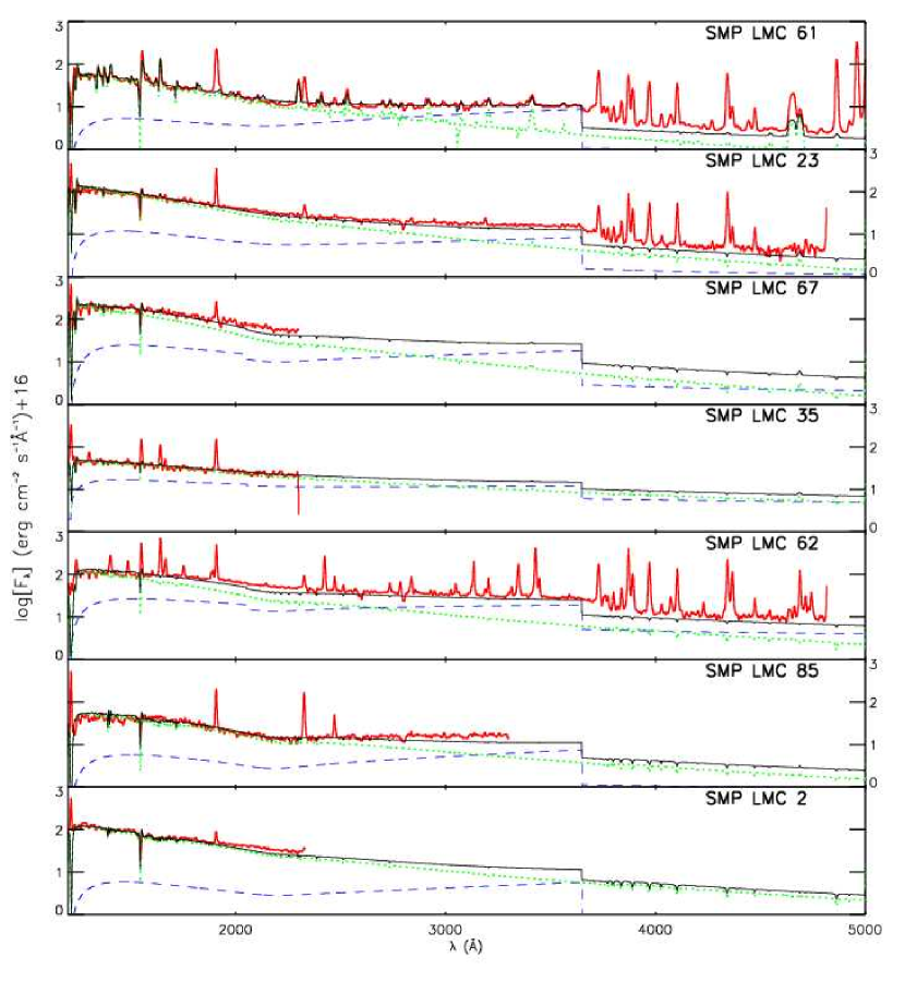
Figure 7: The observations (red/gray) are shown along with our stellar (green/dotted) and nebular continuum models (blue/dashed). The sum of the models is shown by the black solid line. All models have been reddened with our determined values for  $E_{\rm{B-V}}$ (Table 8), and the effects of hydrogen absorption (Table 5) have been applied. The spectra have been convolved with a 5 Å Gaussian for clarity. Note the logarithmic flux scale.

The nebular continuum emission has been modeled using the code described in Bianchi et al. (1997), which accounts for two-photon, H and He recombination, and free-free emission processes. The computed emissivity coefficient of the nebular gas is scaled as an initial approximation to the total flux at the Earth by deriving the emitting volume from the dereddened absolute H$\beta$ flux. In the cases where the spectroscopic aperture was smaller than the nebular size (SMP LMC 35 and 61) the nebular flux was scaled by the corresponding geometrical factor. $T_{e}$ and  $n_{e}$ from the literature are used as initial inputs, and adjusted if necessary. SMP LMC 2 and 85 have no published values of the electron density. For these, we tried different values as inputs and found $\mbox{\,$n_{e}$}=5000$ and 40,000 cm^-3, respectively, to produce satisfactory fits. The high  $n_{e}$ for SMP LMC 85 is consistent with its very compact morphology ($r_{neb}\leq 0.2$ pc). The values of $F_{H\beta}$ and c_Hβ are perhaps the most uncertain, and finally we re-scaled the nebular flux with the assumption that the nebular continuum is responsible for the majority of flux at longer wavelengths (the $H\beta$ fluxes implied by our scaling are listed in bold in the table). This assumption produced an overall good fit of the observed spectra over the entire wavelength range. The nebular continuum is constrained not to exceed the P-Cygni troughs in the UV range. Values of $F_{H\beta}$ listed in parentheses reflect this scaling. Our combined stellar and nebular models, along with the observations, are shown in Fig. 7.

4.3 The Central Stars

As discussed in previous sections, the modeling of the central stars is done concurrently with that of the nebular continuum (§ 4.2) and the hydrogen absorption (§ 4.1). The hot molecular hydrogen along the sight-lines of many of these objects makes the identification of the stellar features in the far-UV and their analysis challenging. For wavelengths shorter than 1200 Å, the nebula does not contribute continuum emission, and this region can be used to set the stellar radius, since the distance is well-established. The reddening has to be derived concurrently, but it is always small, and therefore it does not contribute much to the uncertainties.

4.3.1 The Models

Due to the severe H₂ absorption in the far-UV, there are few photospheric absorption lines are available, so we have relied primarily on wind features to determine the parameters of the CSPN. Intense radiation fields, a (relatively) low wind density, and an extended atmosphere invalidate the assumptions of thermodynamic equilibrium and a plane-parallel geometry for our sample. To model the winds of these objects, we use the non-LTE (NLTE) line-blanketed code CMFGEN of Hillier & Miller (1998, 1999). CMFGEN solves the radiative transfer equation in an extended, spherically-symmetric expanding atmosphere. Originally developed to model the winds of (massive) Wolf-Rayet stars, it has been adapted for objects with weaker winds such as O-stars and CSPN as described in Hillier et al. (2003).

The detailed workings of the code are explained in the references above. In summary, the code solves for the NLTE populations in the comoving-frame of reference. The fundamental photospheric/wind parameters include  $T_{eff}$,  $R_{*}$,  $\dot{M}$, the elemental abundances and the velocity law (including the wind terminal velocity,  v_∞). The stellar radius ( $R_{*}$) is taken to be the inner boundary of the model atmosphere (corresponding to a Rosseland optical depth of $\sim 20$). The temperature at different depths is determined by the stellar temperature  $T_{*}$, related to the luminosity and radius by $L=4\pi\mbox{\,$R_{*}$}^{2}\sigma\mbox{\,$T_{*}$}^{4}$, whereas the effective temperature ( $T_{eff}$) is similarly defined but at a radius corresponding to a Rosseland optical depth of 2/3 ( $R_{2/3}$). The luminosity is conserved at all depths, so $L=4\pi\mbox{\,$R_{2/3}$}^{2}\sigma\mbox{\,$T_{eff}$}^{4}$.

We assumed what is essentially a standard velocity law $v(r)=\mbox{\,v${}_{\infty}$}(1-r_{0}/r)^{\beta}$ where $r_{0}$ is roughly equal to  $R_{*}$. The choice of the velocity law mainly affects the profile shape, not the total optical depth, and does not greatly influence the derived parameters. Once a velocity law is specified, the density structure of the wind $\rho(r)$ is then parameterized by the mass-loss rate  $\dot{M}$ through the equation of continuity: $\mbox{\,$\dot{M}$}=4\pi\mbox{\,$R_{*}$}^{2}\rho(r)v(r)$.

It has been found that models with the same transformed radius  $R_{t}$ [$\propto\mbox{\,$R_{*}$}(\mbox{\,v${}_{\infty}$}/\mbox{\,$\dot{M}$})^{2/3}$] (Schmutz et al., 1989) and  v_∞ have the same ionization structure, temperature stratification (aside from a scaling by  $R_{*}$) and spectra (aside from a scaling of the absolute flux by $\mbox{\,$R_{*}$}^{2}$ — Schmutz et al., 1989; Hamann et al., 1993). Thus, once the velocity law and abundances are set, one parameter may be fixed (say  $R_{*}$) and parameter space can then be explored by varying only the other two parameters (e.g.,  $\dot{M}$ and  $T_{eff}$).  $R_{t}$ can be thought of as an optical depth parameter, as the optical depth of the wind scales as $\propto\mbox{\,$R_{t}$}^{-3}$, for opacities which are proportional to the square of the density. Scaling the model to the observed flux yields  $R_{*}$/$D$. An LMC distance of $D=50.6$ kpc was adopted to determine  $R_{*}$.

4.3.2 Clumping

Radiation driven winds have been shown to be inherently unstable (Owocki et al., 1988, 1994), which should lead to the formation of clumps. The degree of clumpiness is parametrized by $f$, the filling factor. One actually can only derive  $\dot{M}_{S}$=( $\dot{M}_{C}$/$\sqrt{f}$) from the models, where  $\dot{M}_{S}$ and  $\dot{M}_{C}$ are the smooth and clumped mass-loss rates. For the denser winds of population I Wolf-Rayet stars, the clumping factor can be constrained by the strength of the electron scattered line wings, and clumping factors of $f\sim 0.1$ are typical (a reduction of  $\dot{M}$ to roughly a third of its unclumped value). For O-stars, the lower mass loss rates make the electron scattering effects small and difficult to ascertain (Hillier et al., 2003). The winds of our sample stars are even weaker. Given that the wind lines in the far-UV are affected by H₂, and the UV FOS data are not high resolution, we did not attempt to rigorously constrain the degree of clumping in the winds of our sample. We calculated test models with different clumping factors, and generally found the spectrum to be insensitive, except for O VI $\lambda\lambda$ 1032-38 in the hotter models ($\mbox{\,$T_{eff}$}\gtrsim 50$ kK) and P V $\lambda\lambda$1118-28 for cooler models. In some cases, better results were achieved, and such cases are discussed in § 4.3.6. Unless otherwise noted, we have adopted $f=1$ and use  $\dot{M}$ to refer to the smooth mass loss rate throughout this paper. This is an upper limit, and the lower limit of  $\dot{M}$ is estimated to be a third of this value.

4.3.3 Gravity

Because of the severe H₂ absorption in the far-UV, and the masking of the stellar flux by the nebular continuum at longer wavelengths, there are no suitable absorption lines to be used as gravity diagnostics. In CMFGEN, gravity enters through the scale height $h$ ($\propto g^{-1}$), which connects the spherically extended hydrostatic outer layers to the wind. The relation between $h$ and $g$, defined in Hillier et al. (2003), involves the mean ionic mass and mean number of electrons per ion, the local electron temperature and the ratio of radiation pressure to the gravity. Our models typically have scale heights which are equivalent to $\mbox{\,$\log{g}$}\sim 4.7-5.0$. Their hydrostatic structures were verified with test models generated using TLUSTY (Hubeny & Lanz, 1995), which calculates the atmospheric structure assuming radiative and hydrostatic equilibrium, and a plane-parallel geometry, in NLTE conditions. For objects evolving along the constant-luminosity branch and with $40\lesssim\mbox{\,$T_{eff}$}\lesssim 70$ kK (the regime of our objects), evolutionary codes typically adopt $4.0\leq\mbox{\,$\log{g}$}\leq 5.3$ (e.g., Marigo et al., 2002). Over such gravities, the derived wind parameters are not that sensitive to $h$. Spectral wind features can be fit with the models of the same  $T_{eff}$ but with gravities differing by over a magnitude. In such cases, the lower gravity model requires a higher luminosity, as its more extended atmosphere results in larger discrepancy between  $T_{*}$ and  $T_{eff}$. To illustrate the impact of adopting a different  $\log{g}$ on the derived parameters, a model with $\mbox{\,$T_{eff}$}=55$ kK, $\mbox{\,$\log{g}$}\simeq 5$, $L\simeq 5000$  $\rm{L_{\odot}}$, and $\mbox{\,$R_{*}$}\simeq 0.8$  $\rm{R_{\odot}}$ produces about the same spectrum as a model with the same  $T_{eff}$, but with $\mbox{\,$\log{g}$}=4$, and $L$ about 8 % larger and  $R_{*}$ about 17 % smaller. For gravities stronger than $\mbox{\,$\log{g}$}\simeq 5.0$, the discrepancy is smaller, for lower gravities, larger. For $\mbox{\,$\log{g}$}=3.7$,  $R_{*}$ is $\sim 30$ % smaller and and $L$ is about $\sim 20$ % greater. Thus, for our hotter objects (i.e., $\gtrsim 50$ kK) we estimate the errors due to uncertainty of the gravity to be $\lesssim 20$ % for the radius and $\lesssim 10$ % for the luminosity. For cooler objects, the errors are estimated to be $\lesssim 30$ % for the radius and $\lesssim 20$ % for the luminosity.

4.3.4 Abundances

CSPN can be generally divided into two groups based on surface abundances: Hydrogen-rich (those that show obvious Hydrogen lines in their spectra, and exhibit “normal” abundances) and Hydrogen-deficient (which don’t). The H-rich objects are thought to be in a quiescent Hydrogen-burning phase, and the H-deficient stars in a post-Helium flash, Helium-burning phase. About 10-20 % of CSPN are H-deficient (De Marco & Soker, 2002; Koesterke & Werner, 1998 and references therein). This class includes [WC] objects. It seems the two groups represent different “channels” of CSPN evolution, terminating with either H-rich or He-rich white dwarfs (DA or DO) (see Napiwotzki, 1999 for a discussion).

To model these CSPN, we constructed two grids of models, ranging in  $T_{eff}$ from 30–80 kK and in $\mbox{\,$R_{t}$}\sim$ 3–200  $\rm{R_{\odot}}$. The first, appropriate for “H-rich” CSPN, have solar abundances for H and He but assume an LMC metallicity of $z=0.4$  $\rm{Z_{\odot}}$ for the metals. For the second, corresponding to “H-deficient” (or H-poor) CSPN, we have considered the following. It has been shown that, throughout the [WC] subclasses, the spectroscopic differences are mainly tied to  $\dot{M}$ and  $T_{eff}$, rather than to the abundances (Crowther et al., 1998, 2002). The abundances throughout the [WC] subclasses are about constant, with typical values of (by mass)  $X_{He}$= 0.33–0.80,  $X_{C}$= 0.15–0.50,  $X_{O}$= 0.06–0.17 (De Marco & Barlow, 2001). The abundance patterns of PG 1159-[WC] and PG 1159 stars, the likely descendants of the [WC] class, are similar (Werner, 2001). For these reasons, we have assumed for the second grid a similar abundance pattern of  $X_{He}$/ $X_{C}$/ $X_{O}$= 0.55/0.37/0.08 and an LMC metallicity of $z=0.4$  $\rm{Z_{\odot}}$ for the other elements (e.g., S, Si, & Fe). The nitrogen abundance in these objects typically ranges from none to $\sim$2% in Galactic objects, we have adopted $\sim$1% (by mass). The abundances for the H-rich and H-deficient grids summarized in Table 7. We note here that throughout this work, the nomenclature $X_{i}$ represents the mass fraction of element $i$, and ‘ $\rm{X_{\odot}}$” denotes the solar value.

Strictly speaking, “H-rich” CSPN are those which display detectable hydrogen in their spectra. Even in the optical, hydrogen abundances are often difficult to measure in these objects because hydrogen features are often masked by those of He II (see Leuenhagen & Hamann, 1998 for a discussion). We emphasize here that there are no diagnostics in the far-UV or UV spectra of our objects that allow us to make a statement regarding their hydrogen abundance. The handful of wind lines upon which we are basing our parameter determinations do not allow us to make firm statements regarding their abundances.

For the model ions, CMFGEN utilizes the concept of “superlevels”, whereby levels of similar energies are grouped together and treated as a single level in the rate equations (Hillier & Miller, 1998). Ions and the number of levels and superlevels included in the model calculations, as well references to the atomic data, are given in the Appendix (§ A).

4.3.5 Diagnostics

The terminal velocity ( v_∞) can be estimated from the blue edge of the P-Cygni absorption features (Table 3), preferably those that form further out in the wind. However, strong P-Cygni profiles obscured by H₂ absorption or nebular emission are rare in the far-UV spectra of our sample. Some of these are more reliable than others: H₂ absorption makes the C III $\lambda$977 measurement questionable if it is weak, and, if strong, the blue edge of its trough is obscured by Ly$\gamma$ airglow. Ly$\beta$ airglow and H₂ absorption similarly affect the O VI doublet. Furthermore, the components of the O VI doublet are not optimal estimators of  v_∞ because O VI typically forms deep in the wind. We usually used C IV $\lambda\lambda$1548-51 for our first guess of  v_∞, and adjusted this value to match the wind lines. Our final derived velocities will be presented in § 4.3.6 and listed in Table 8.

The scarcity of strong wind features of these objects poses some difficulty in their modeling. Typically, one determines  $T_{eff}$ by the ionization balance of the CNO elements. For these objects, we typically use C III/C IV and/or O IV/O V/O VI to constrain  $T_{eff}$. It is desirable to use diagnostics from many elements to ensure consistency. The presence or absence of some features offer further constraints. For example, for mass-loss rates in the regime of our stars, Si IV $\lambda\lambda$1394,1402 disappears at temperatures $\mbox{\,$T_{eff}$}\gtrsim 50$ kK, S IV $\lambda\lambda$1062, 1075 at $\sim$45 kK, and P V $\lambda\lambda$ 1118-28 at $\sim$60 kK. We generally use all wind lines to constrain  $\dot{M}$.

We adopted the following method. We compared the observed spectra with the theoretical spectra of our model grids to determine the stellar parameters  $T_{eff}$ and  $R_{t}$. far-UV and UV flux levels were used to set  $R_{*}$ (since the distance is known), and from that  $\dot{M}$ and the $L$ can be derived. If necessary, models with adjusted abundances are calculated. Uncertainties in the quoted parameters reflect the range that the parameters must be varied to fit the diagnostics.

4.3.6 Stellar Modeling Results

From our spectral fitting process we determined the distance-independent parameters  $T_{eff}$,  $R_{t}$, and  v_∞. Once a distance is adopted,  $R_{*}$ was derived by scaling the model flux to the observations, and then $L$ and  $\dot{M}$ were determined. Our derived central star parameters are summarized in Table 8, along with masses estimated by comparing our parameters to the evolutionary tracks of Vassiliadis & Wood (1994), and the resulting gravities. We list our smooth (unclumped) mass-loss rates  $\dot{M}_{S}$ (corresponding to $f=1.0$), and a clumped rate  $\dot{M}_{C}$ (corresponding to $f=0.1$). We have presented our unclumped models in the figures, but as noted in § 4.3.6, the clumped rates are also generally consistent with the observations. We also list the ratio of the luminosity to the Eddington luminosity ($\Gamma$), and indicate which model abundances were used for each object — SMP LMC 61 was fit using He/C/O rich abundances typical of “H-deficient” (H-poor) objects, and the others with normal, LMC abundances (expected for “H-rich” CSPN). Noticeable trends that go with increasing effective temperatures are higher terminal velocities, smaller radii, and lower mass-loss rates. These are generally expected from our current ideas about CSPN evolution — as the object loses mass as it evolves along the constant-luminosity portion of the HRD, it contracts and gets hotter (e.g., Acker & Neiner, 2003).

Also listed in Table 8 are reddenings determined from fitting the multiple components to the far-UV/UV spectra (these are generally in good agreement with those derived from the Balmer decrement, shown in Table CENTRAL STARS OF PLANETARY NEBULAE IN THE LARGE MAGELLANIC CLOUD: A FAR-UV SPECTROSCOPIC ANALYSIS).

We now discuss the modeling results for our sample objects.

SMP LMC 61 (Fig. 8): This object was classified as a [WC4/5] by Monk et al., 1988 based on its optical spectrum. Our model, with $\mbox{\,$T_{eff}$}\simeq 70$ kK, $\mbox{\,$\dot{M}$}\simeq 4.7\mbox{\,$\rm x10^{-7}$}$  $\rm{M_{\odot}\>yr^{-1}}$, and $\mbox{\,v${}_{\infty}$}\simeq 1300$  $\rm{km\>s^{-1}}$ and the He/C/O-rich (H-deficient) abundances discussed in § 4.3.4 fit most diagnostics satisfactorily, with the exceptions discussed below. Our final abundances for this star are listed in Table 10.

Our model (which is unclumped) produces a C IV $\lambda\lambda$1548-51 weaker than the observed one. Crowther et al. (2002) had similar problems in their analysis of Galactic WC4 stars. They found the radial velocity of the C IV profile to be sensitive to clumping in the wind and achieved better fits with filling factors of $0.1\leq f\leq 0.01$. We have computed models with $f=0.1$ and 0.01 to test the effects of clumping for this [WC] object, and find C IV to also be sensitive to this parameter. While the fit of this feature is improved, it is still not fit satisfactorily in either case.

The C III $\lambda$1247 feature may be blended with N V 1238-43. Our model, which assumed a nitrogen mass fraction of 1%, produced a nitrogen emission which is too strong (presented in the figure). A model with no nitrogen (typical of an atmosphere of a massive WC star) produces better agreement with the observations, although it cannot be definitively said the nitrogen abundance is zero.

Finally, with an iron abundance 0.4 the solar value, the Fe VI spectrum (spanning 1250–1350 Å) was too strong. In cooler models, the Fe V spectrum is too strong (appearing between 1350–1500 Å). Hotter models produced unobserved Fe VII and Fe VIII features in the UV and far-UV, respectively (see Herald & Bianchi, 2004a for a more detailed discussion of using the iron spectrum as a diagnostic for CSPN). Smaller mass-loss rates fail to match the non-iron diagnostics. We were able to match the iron spectrum by lowering its abundance to 1/10th the LMC metallicity ( $X_{Fe}$= 5.44 $\rm x10^{-5}$ by mass). The other diagnostics are not sensitive to the iron abundance, and removing iron from the model wind has no significant impact on the synthetic spectrum (except for O V $\lambda$1371, which lies among the iron spectrum). This implications of this iron deficiency will be discussed more in § 5.

Bianchi et al. (1997) modeled the central star of LMC 61 using a blackbody distribution to determine parameters of $\mbox{\,$T_{eff}$}=60$ kK, $\mbox{\,$R_{*}$}=0.95$  $\rm{R_{\odot}}$, and $L\simeq 10^{4}$  $\rm{L_{\odot}}$, and $\mbox{\,$\dot{M}$}=7\mbox{\,$\rm x10^{-7}$}$  $\rm{M_{\odot}\>yr^{-1}}$ from a wind-line analysis. However, they had difficulty in modeling all parts of the spectrum simultaneously without invoking an additional component (a cooler companion). They relied on FOS data, which have flux levels in excess of the more recent STIS spectrum which we utilize (the STIS and FUSE levels are in good agreement).

More recently, Stasińska et al. (2004) modeled the stellar UV/optical spectra LMC 61 in conjunction with photoionization models of the nebula, and determined the central stars parameters: $\mbox{\,$T_{*}$}=88$ kK, $\mbox{\,$R_{*}$}=0.42$  $\rm{R_{\odot}}$, $\log{L}=3.96$  $\rm{L_{\odot}}$, $\log{\mbox{\,$\dot{M}$}}=-6.12$  $\rm{M_{\odot}\>yr^{-1}}$, with He/C/O = 0.45/0.52/0.03. Their mass-loss rate agree with ours (within the uncertainties), but they find a higher luminosity and temperature. However, they were not able to simultaneously fit the observed spectrum and nebular ionizing fluxes, noting that the nebular analysis requires a central star luminosity of $\log{L}=3.66$  $\rm{L_{\odot}}$ (in line with our findings). The higher temperature they derived appears to be due to choice of diagnostics. For example, they fit C IV $\lambda\lambda$1548-51 well (which we do not) but not C III 1175 (which we do). They, too, found that a sub-LMC iron abundance was needed to match the spectrum of this object.

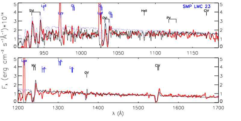
Figure 9: SMP LMC 23: Description follows that of Fig. 8.

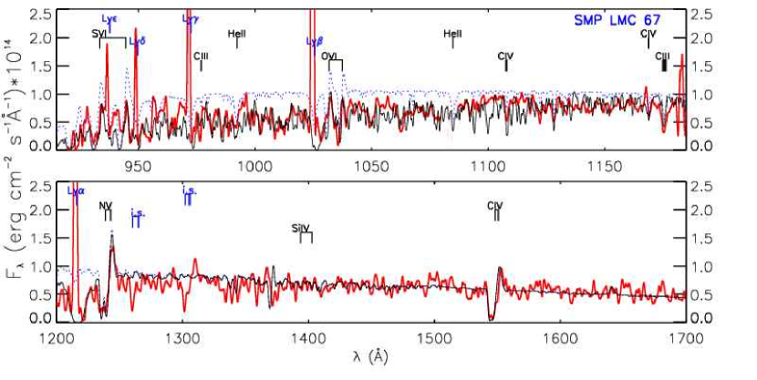
Figure 10: SMP LMC 67: Description follows that of Fig. 8. The theoretical nebular continuum (§ 4.2) has been subtracted from the UV observations.

SMP LMC 23 and 67 (Figs. 9 and 10): As noted before, the spectra of SMP LMC 23 and SMP LMC 67 are similar (except for C III $\lambda$1175), and we derive similar parameters: $\mbox{\,$T_{eff}$}=60$ kK, $\mbox{\,$\dot{M}$}=3.8\mbox{\,$\rm x10^{-8}$}$  $\rm{M_{\odot}\>yr^{-1}}$ and $\mbox{\,$T_{eff}$}=55$ kK, $\mbox{\,$\dot{M}$}=4.5\mbox{\,$\rm x10^{-8}$}$  $\rm{M_{\odot}\>yr^{-1}}$, respectively. We fit both adequately using models of normal LMC abundances (i.e., “H-rich”). SMP LMC 67 is a bit hotter, as evidenced by stronger O VI and lack of C III $\lambda$1175. The far-UV flux of both objects suffer significant absorption due to hot H₂, which can be appreciated by comparing the models before and after the absorption effects are applied in the figures. In the UV, the nebular continuum contributes a bit to the flux for SMP LMC 67. For these objects, clumped models with filling factors of $f=0.1$ showed little change in the emergent spectra, with only O VI 1032-38 weakening slightly.

Bianchi et al. (1997) modeled the central star of SMP LMC 67 using a blackbody distribution and determined $\mbox{\,$T_{eff}$}=45$ kK, $\mbox{\,$R_{*}$}=1.06$  $\rm{R_{\odot}}$, and $L=4157$  $\rm{L_{\odot}}$ (versus our values of $\mbox{\,$R_{*}$}=0.80$, $L\simeq 5000$  $\rm{L_{\odot}}$).

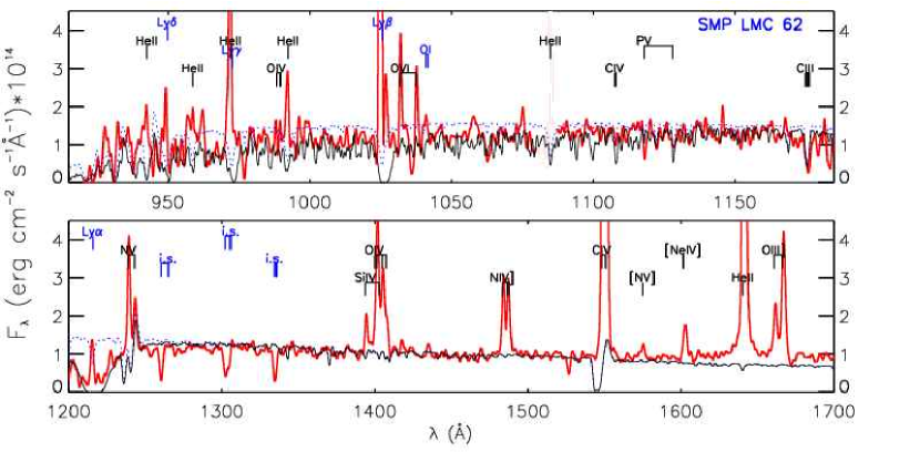
Figure 11: SMP LMC 62: Description follows that of Fig. 8.

SMP LMC 62 (Fig. 11): The FUSE spectrum of SMP LMC 62 is mostly the fingerprint of hot ($T\gtrsim 3000$) H₂. Even what appears to be a P-Cygni profile for the O VI doublet might be an artifact of the H₂ absorption. Once the H₂ is accounted for, there are no obvious strong wind features detectable in the far-UV. S VI $\lambda\lambda$933-44 is not obviously present. C III $\lambda$1175 appears in absorption, but it may have an interstellar contribution (Danforth et al., 2002 found C III absorption associated with LMC material along many of the LMC sight-lines presented in their comprehensive atlas). C IV $\lambda$1107 and P V $\lambda\lambda$1118-28 seem to be present, but because of the H₂ absorptions which completely blanket the FUSE range, a definitive statement is not possible. The nebular emission features in the FOS range make it difficult to discern any stellar features except for, perhaps, N V $\lambda\lambda$1238-43. Thus, this star has fewer diagnostics to work with than the others of our sample. We have assumed H-rich abundances for this object, however, due to the lack of stellar features, abundances cannot be firmly constrained. C III $\lambda$1175 and the absence of strong S VI $\lambda\lambda$933-44 place a rough upper limit on  $T_{eff}$ of $\lesssim 55$ kK. The presence of fairly strong N V $\lambda$1240 requires $\mbox{\,$T_{eff}$}\gtrsim 40$ kK, and imposes a rough lower limit to  $\dot{M}$. Our model adequately fits the emission of this feature, but because the nebular emission obscures the absorption trough,  v_∞ is difficult to constrain. P V and C III appear in absorption, restricting  $\dot{M}$. The absence of O IV $\lambda\lambda$1339-43 and O V 1371 also places upper limits on  $T_{eff}$ and  $\dot{M}$. Thus, we estimate $\mbox{\,$T_{eff}$}=45\pm 5$ kK, $\mbox{\,$\dot{M}$}\simeq 2\mbox{\,$\rm x10^{-8}$}$  $\rm{M_{\odot}\>yr^{-1}}$, and $\mbox{\,v${}_{\infty}$}\simeq 1000$  $\rm{km\>s^{-1}}$ for this star.

As discussed in § 4.1, the extremely high temperature required to fit the H₂ absorptions suggests non-equilibrium conditions in the nebular environment, which might arise from shocks. This sight-line to this star also has a relatively high H I column density [$\mbox{\,$\log{N}$}(\mbox{\rm{{H~{}I}}})\simeq 21.7$] with respect to the others of our sample. The reddening corresponding to this column density for a typical interstellar dust/gas ratio is much higher than what we determine from our continuum fits ($\mbox{\,$E_{\rm{B-V}}$}\simeq 1$ vs. 0.1 — see Tables 5 and 8). This implies that the majority of H I along the sight-line is probably circumstellar.

Previous photoionization models of the UV nebular spectrum (discussed in § 5) have predicted a significantly higher temperature for this star than our result (127 vs. 45 kK). Central star temperatures of $\mbox{\,$T_{eff}$}>125$ kK produce nebular O VI $\lambda\lambda$1032-38 through photoionization (Chu et al., 2004), so such a temperature would be consistent with our observations of this feature. Our low stellar temperature can be reconciled with the highly-ionized nebular spectrum if shocks (suggested by the H₂ features) are responsible for the nebular ionization. However, in shock excited gas [Ne V] 3426 is invariably much weaker than O VI $\lambda$1032. Therefore our observations seem to rule out shocks as the source of the [Ne V] emission. In contrast, photoionization models of high excitation PN (Otte et al., 2004) predict a [Ne V] 3426 to O VI 1032 ratio of about 7, which is similar to what we observe.

Test stellar atmosphere models at the photoionization temperature ($\mbox{\,$T_{eff}$}=127$ kK) do not reproduce C III $\lambda$1175 or P V $\lambda\lambda$1118-28 (although the former could be interstellar and the latter cannot be clearly seen due to H₂ absorptions). For this temperature, the observed far-UV flux levels imply $\mbox{\,$R_{*}$}\simeq 0.5$  $\rm{R_{\odot}}$ and $\log{L}\simeq 4.7$  $\rm{L_{\odot}}$, an extremely luminous CSPN (most LMC CSPN have $\log{L}\lesssim 3.9$  $\rm{L_{\odot}}$, e.g., Dopita & Meatheringham, 1991a, b). This luminosity correspond to current mass of $\sim$1.2  $\rm{M_{\odot}}$ (according to the tracks of Paczyński, 1970) and is comparable to that of LMC N 66 (SMP LMC 83), a WN-type object which displayed a dramatic outburst in 1993 and the nature of which remains unclear (Hamann et al., 2003). Thus, the results of our stellar modeling are not consistent with parameters derived from nebular analysis, and the discrepancy is not clarified by the present data. CSPN with winds and high temperatures such as the photoionization temperature of this object typically belong to a class of objects termed “O VI PN nuclei”, which exhibit emission lines of O VI $\lambda\lambda$3811-34 and, often, C IV $\lambda\lambda$5801-12. Thus optical spectroscopy of the central star could help resolve the discrepancy.

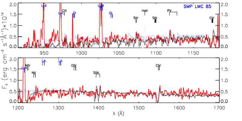
Figure 12: SMP LMC 85: Description follows that of Fig. 8.

SMP LMC 85 (Fig. 12): This is one of the dimmer objects in our sample (it is more reddened). The far-UV spectrum of this object is somewhat contaminated with airglow lines, and features at shorter wavelengths should be viewed with caution due to the small effective area of the FUSE SiC detectors. However, one can still recognize C III $\lambda$977, S IV $\lambda$1072, P V $\lambda\lambda$1118-28 and perhaps O VI $\lambda\lambda$ 1032-38 and C III $\lambda$1175 in the far-UV. In the UV, the Si IV and C IV doublets are present, and perhaps O IV $\lambda\lambda$1339-43 (the FOS data are noisy also). The P V, S IV, and Si IV lines indicate a cooler object with a lower terminal velocity. We derive $\mbox{\,$T_{eff}$}=40\pm 2$, $\mbox{\,$\dot{M}$}\simeq 4-16\mbox{\,$\rm x10^{-8}$}$  $\rm{M_{\odot}\>yr^{-1}}$, $\mbox{\,v${}_{\infty}$}\simeq 700$  $\rm{km\>s^{-1}}$, and are able to fit its spectrum adequately using LMC abundances.

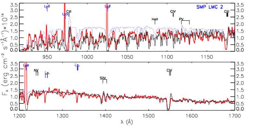
Figure 13: SMP LMC 2: Description follows that of Fig. 8.

SMP LMC 2 (Fig. 13): This object has strong C III signatures in the far-UV (both $\lambda$977 and $\lambda$1175). Once the (hot) H₂ absorption is taken into account, it appears the O VI doublet is not present. The UV spectrum shows modest N V, Si IV and C IV doublets. We derive $\mbox{\,$T_{eff}$}\simeq 38$ kK, $\mbox{\,$\dot{M}$}\simeq 3\mbox{\,$\rm x10^{-8}$}$  $\rm{M_{\odot}\>yr^{-1}}$, and $\mbox{\,v${}_{\infty}$}\simeq 700$  $\rm{km\>s^{-1}}$ using LMC abundances. In our unclumped model, P V $\lambda\lambda$1118-28 is a bit strong. A clumped model with $f=0.1$ resulted in the P V feature to weaken enough to agree with the observations, while leaving the other wind features unchanged significantly (we present the unclumped model in the figure, for consistency with the other objects).

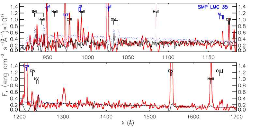
Figure 14: SMP LMC 35: Description follows that of Fig. 8.

SMP LMC 35 (Fig. 14): The dimmest object of our sample, LMC 35 is shown in Fig. 14. The data has the lowest S/N, and has been heavily smoothed. Many features, especially at the shorter wavelengths covered by FUSE, are dubious. Given the poor quality of the data, we did not attempt a rigorous fit of the stellar spectra. We present a model of $\mbox{\,$T_{eff}$}=50$ kK, $\mbox{\,$\dot{M}$}=1\mbox{\,$\rm x10^{-8}$}$  $\rm{M_{\odot}\>yr^{-1}}$, and $\mbox{\,v${}_{\infty}$}=1000$  $\rm{km\>s^{-1}}$ that is produces an acceptable fit. The data are, however, good enough to see that hot H₂ lies along this objects sight-line.

5 DISCUSSION

Our sample PN are compact, and thus relatively young. Our derived effective temperatures ($38\lesssim\mbox{\,$T_{eff}$}\lesssim 70$ kK) are on the cooler side for CSPN. The sample also show a small spread in luminosity. For comparison, temperatures derived from photoionization models (Dopita & Meatheringham, 1991a, b; Dopita et al., 1997; Vassiliadis et al., 1998b) are listed in Table 9. Our derived temperatures are in good agreement with those of the photoionization models, with the exception of SMP LMC 62 (and SMP LMC 35, which we did not fit). For SMP LMC 62, we derive a significantly lower temperature than the photoionization temperature (45 vs. 127 kK — discussed in § 4.3.6).

Comparing our temperatures and luminosities with the $z=0.008$ evolutionary tracks of Vassiliadis & Wood (1994) (appropriate for the metallicity of the LMC), we find our sample luminosities are a bit low for the H-burning tracks, and fall more naturally on their He-burning tracks. Comparing with the latter, our hotter objects (i.e., $\mbox{\,$T_{eff}$}\gtrsim 45$ kK) fall between the initial-final mass tracks of ($M_{i},M_{f}$) = (2.0,0.669) and (1.5,0.626)  $\rm{M_{\odot}}$, with evolutionary ages of 1-3 kyr. The cooler objects lie within the (1.0,0.578) and (0.95,0.554)  $\rm{M_{\odot}}$ tracks, also with evolutionary ages of 1-3 kyr. These evolutionary ages, $\tau_{evol}$, are listed in Table 9 along with the dynamical ages calculated from $\tau_{dyn}=r_{neb}/v_{exp}$ using the values from Table CENTRAL STARS OF PLANETARY NEBULAE IN THE LARGE MAGELLANIC CLOUD: A FAR-UV SPECTROSCOPIC ANALYSIS. Note that the kinematic age is expected to be a lower limit to the post-AGB age, as the nebular expansion is thought to increase during the early post-AGB phase and then level off as the nucleus fades (see Sabbadin, 1984, Bianchi, 1992 and references therein). Generally, the dynamic and evolutionary ages are in good agreement, not differing by more than a factor of two. It is not surprising that most of the objects are on the massive side. This is because the brightest known objects were chosen for the FUSE program since their fluxes are at the lower limits of the FUSE sensitivity.

The low mass-loss rates of these objects and their lack of diagnostics make the abundances difficult to constrain. For most objects, we are able to fit their spectra using normal LMC abundances (corresponding to H-rich CSPN). H-rich CSPN can be either H- or He-burning, but comparison with the evolutionary tracks indicate that these objects are most probably He-burners.

SMP LMC 61, the [WC4] star, is fit using He/C/O enriched abundances that only He-burners are expected to display. We also find an iron deficiency for this object (as do Stasińska et al., 2004). Werner et al. (2002) and Herald & Bianchi (2004a) have found iron deficiencies in Galactic PG 1159-[WC] stars (these stars are thought to represent a phase where the CSPN is transitioning between a [WC] star and PG 1159 star, an entry point onto the WD cooling sequence). Miksa et al. (2002) have also found iron deficiency in a large sample of (Galactic) PG 1159 stars, the supposed descendants of these transitional objects. Iron deficiencies in these objects may result when material in the He-intershell is exposed to $s$-process nucleosynthesis during a thermally pulsating AGB or post-AGB phase (Lugaro et al., 2003; Herwig et al., 2003). Iron deficiency in [WC] stars is very interesting from the standpoint of radiation-driven winds. For massive WR stars, the opacity of the wind from iron and iron-group elements is thought to play a crucial role in initiating the driving of the wind (Lamers & Nugis, 2002; Crowther et al., 2002). The iron opacity of these optically thick line driven winds plays an important role in determining where the sonic point occurs, which in turn dictates the characteristics of the wind (e.g.,  $\dot{M}$) (Lamers & Nugis, 2002). Wind density is the primary discriminator between the (massive) WC4-7 subtypes (Crowther et al., 2002). In contrast to massive WC stars, there is a known lack of [WC5-7] subtypes among CSPN, which is not understood (e.g., Crowther et al., 2002 and references therein). If [WC] winds are similarly sensitive to the iron opacity, an iron deficiency in these winds might be related to the dearth of [WC5-7] subtypes among CSPN.

Vink et al. (2001) presented mass-loss rate predictions for massive O and B stars of different metallicities. Their models yield mass-loss rates for given stellar parameters, taking into account opacity shifts in the wind due to different ionization structures at different temperatures (assuming “normal”, i.e., non-enriched, abundances). We tested their relation for our low-mass objects using our derived stellar parameters ( $T_{eff}$, $L$,  v_∞, and  $\log{g}$) from Table 8 with our adopted metallicity of $z=0.4\mbox{\,$\rm{Z_{\odot}}$}$ (note that SMP LMC 61 has chemically processed atmosphere, so the Vink prescription does not apply in this case). The results (listed in Table 9) show, on average, the predicted mass-loss rates to be $\sim 3$ times lower than our derived (smooth-wind) rates. However, a clumping factor of $f=0.1$ (which is consistent with observations in most cases and produce better fits in some — § 4.3.6) would reduce our mass-loss rates sufficiently to bring them into rough agreement with the Vink et al. (2001) values.

Also listed in Table 9 for our objects are the ratios of the wind momentum flux to the radiative momentum flux (the “performance numbers”), defined as $\eta=\mbox{\,v${}_{\infty}$}\mbox{\,$\dot{M}$}c/L$ (Springmann, 1994), calculated using the parameters in Table 8. A performance number of unity corresponds to the case where each photon, on average, scatters once in the wind (the “single scattering limit”). A performance number of $>1$ indicates photons are scattering multiple times, requiring a higher wind opacity. For all the objects of our sample, $\eta\lesssim 1$ except for SMP LMC 61, which has $\eta\simeq 7$. There are indications that the wind of the latter object is clumped (4.3.6) which would reduce  $\dot{M}$. But the wind would have to be highly clumped ($f<0.01$) to reduce $\eta$ below unity (it was not necessary to invoke clumping to fit the profiles of the LMC-abundance objects). The larger performance number for the [WC] object reflects the higher opacity of its chemically enriched wind, which makes the wind more efficient at capturing radiation momentum.

Acker & Neiner (2003) analyzed and classified 42 Galactic [WR] objects, which included 7 [WC4] stars. Their average effective temperature was the same as for our LMC [WC4] star, SMP LMC 61 (70 kK). But their average terminal velocity was almost twice as high (2300 vs. 1300  $\rm{km\>s^{-1}}$). As the [WR] evolves through the constant-$L$ phase, $\mbox{\,v${}_{\infty}$}/\mbox{\,$\dot{M}$}$ is roughly constant and  v_∞ correlates with  $T_{eff}$ (e.g., Leuenhagen & Hamann, 1998 and references therein). Thus the lower  v_∞ of our LMC object with respect to Galactic objects of similar  $T_{eff}$ and $L$ probably is an effect of the lower LMC metallicity.

To further investigate the effects of metallicity on the radiative driving, we computed the modified wind momentum $\Pi\equiv\mbox{\,$\dot{M}$}\mbox{\,v${}_{\infty}$}\mbox{\,$R_{*}$}^{0.5}$ for our sample CSPN, also listed in Table 9. Radiative wind driven theory predicts $\Pi\propto Z^{1.0}$. For Galactic (massive) O and B-stars, there is a clear correlation between $L$ and $\Pi$. Lamers et al. (1996) have shown that Magellanic Cloud O and B stars of equivalent luminosities do indeed tend to have lower modified wind momenta, although not quite as low as predicted by theory.

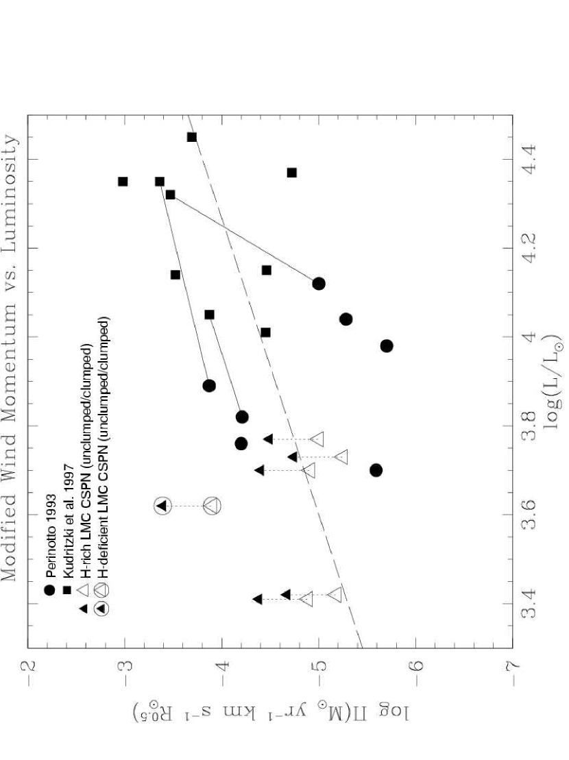
Figure 15: Luminosity vs. Modified Wind Momentum: The Galactic samples of Perinotto (1993) and Kudritzki et al. (1997) are shown (solid circles and squares, respectively). Solid lines join stars appearing in both Galactic samples. We also show our LMC sample, with parameters corresponding to smooth and clumped winds (filled and unfilled triangles, connected by dotted line). SMP LMC 61, the [WC] star, is denoted by the circled triangles. (unfilled triangle). The luminosity-modified wind momentum relation for Galactic O-stars, extrapolated to CSPN luminosities, is shown by the dashed line (from Tinkler & Lamers, 2002).

Tinkler & Lamers (2002) calculated $\Pi$ for the H-rich CSPN samples of Kudritzki et al. (1997) and Perinotto (1993), and extrapolated the luminosity-wind momentum relation for Galactic O-stars down to CSPN luminosities. They found the H-rich CSPN to be clustered into two groups, with higher and lower $\Pi$s than predicted by the relation, respectively, but with about the same slope. In Fig. 15, we plot these Milky Way samples with our objects, with both our unclumped mass-loss rates, and mass-loss rates corresponding to a clumping factor of $f=0.1$. Our objects extend the high-$\Pi$ group to lower luminosities, but basically follow the same relation. In other words, they do not show systematically lower wind momenta as predicted for their lower metallicity. Possible explanations include that the wind momentum-luminosity for massive OB stars is not valid for lower CSPN luminosities and/or our luminosities are underestimated from our lack of knowledge of  $\log{g}$ (see § 4.3.3). To expand on the former, Tinkler & Lamers (2002) attempted to reconcile the differences between the Kudritzki et al. (1997) and Perinotto (1993) samples by scaling their parameters to make them consistent (although, they admit, not necessarily correct). Investigating the wind momentum-luminosity relationship with this rescaled set, they concluded that, for CSPN, the wind momentum seemed to depend more on  $T_{eff}$ than on $L$. If that is correct, metallicity may have less of an impact on the evolution of low/intermediate mass stars than on massive ones. However, it should be noted that all three samples (Perinotto, 1993, Kudritzki et al., 1997, this work) were analyzed using different methods that are not consistent (note the difference of parameters for NGC 6826 and IC 418, which appear in both Galactic works). In particular, Tinkler & Lamers (2002) note that the Kudritzki et al. (1997) sample most likely overestimates  $R_{*}$ (and hence,  $\dot{M}$ and $L$) due to their reliance on the H$\gamma$ line as a diagnostic. The root of the discrepancies seen among the Galactic samples are also due to distance uncertainties, a problem that does not affect our LMC sample.

All of our objects have very hot molecular hydrogen ($T\sim 2000$ K) along their sight-lines, presumably associated with their circumstellar environment. Herald & Bianchi (2002) found a H₂ gas of $T\simeq 1250$ K around the (more evolved) Galactic CSPN of Abell 35, and Herald & Bianchi (2004a) found H₂ temperatures of $\sim 300$ K for four other Galactic CSPN. The higher H₂ temperatures found in our LMC objects may be because they are compact, thus more likely a shocked environment (as indicated by SMP LMC 62) and/or because the H₂ is closer to the star. H₂ may exists in clumps, shielded from the intense UV radiation fields by neutral and ionized hydrogen, as appears to be the case in the Helix nebula (Speck et al., 2002). Speck et al. (2002) suggest that these clumps may form after the onset of the PN phase, arising from Rayleigh-Taylor instabilities at either the ionization front or the fast wind shock front. It could be that this happened in the recent enough past history of these young PN that the H₂ has not returned to its equilibrium state.

As noted in § 4.1, our measured column densities of H I (from the Ly$\alpha$ and Ly$\beta$ profiles) are higher than those determined by applying a typical interstellar gas-to-dust relation (such as that of Bohlin et al., 1978) to our derived reddenings (listed in Table 5). Assuming that the difference represents the circumstellar H I column, we calculated the circumstellar H I mass for a variety of simple shell geometries. Because the H I column density is higher (a few order of magnitudes) than the H₂ column density, and the typical mass of the ionized gas is negligible, we can assume that the neutral hydrogen accounts for the difference between the initial mass (inferred from the evolutionary tracks, § 5) and the mass of the remnant (Table 8). In all but one case the comparison suggests the H I to be located in a volume larger than (or outside of) the ionized shell. The exceptional case is SMP LMC 62, where the H I seems confined within a comparable radius to the ionized gas.

6 CONCLUSIONS

We have analyzed FUSE observations of seven central stars of bright, compact planetary nebulae in the LMC. Most objects display definite wind features, and we determined their stellar parameters using the stellar atmosphere code CMFGEN to analyze their FUSE far-UV and HST UV spectra. We also modeled the nebular continua (which contributes to the UV flux) and the atomic and molecular hydrogen absorption along the sight-line (which severely affects the far-UV spectra).

By virtue of their membership of the LMC, the uncertainties in the distances is small. This is a great advantage over Galactic CSPN, where the distance is the largest source of uncertainty in the analysis. The objects have a spread of effective temperatures between 35 and 70 kK, with mass-loss rates of $\mbox{\,$\dot{M}$}\sim 5\mbox{\,$\rm x10^{-8}$}$  $\rm{M_{\odot}\>yr^{-1}}$ (the one [WC] star has a mass-loss rate an order of a magnitude larger). Terminal wind velocities generally increase with increasing effective temperatures, and range between 700—1300  $\rm{km\>s^{-1}}$, a factor of two lower than Milky Way counterparts. Radii decrease with increasing temperature, as expected. Their luminosities are similar ($L\sim 4000$  $\rm{L_{\odot}}$), and the parameters of the CSPN fall on the He-burning evolutionary tracks of Vassiliadis & Wood (1994), from which we infer post-AGB ages in good agreement with the estimated dynamical ages.

We modeled five of the objects with typical LMC abundances ($z=0.4$  $\rm{Z_{\odot}}$). For these, we investigated the effects of the lower LMC metallicity on the wind acceleration by calculating the modified wind momentum. Contrary to what is expected based on radiative driven wind theory, we did not find any substantial deviation from the wind momentum-luminosity relation that holds for Galactic O and B stars, and roughly holds for Galactic CSPN stars, but the scatter is comparable to the expected difference. Whether this is because the wind momentum does not as simply depend on the luminosity for CSPN as for O and B stars (as suggested by Tinkler & Lamers, 2002) or because of some other effect is unclear.

The one [WC] star of our sample, SMP LMC 61, was modeled using typical He/C/O enriched abundances (products of He-burning). We also determined a sub-LMC iron abundance (also found by Stasińska et al., 2004), perhaps a product of $s$-process nucleosynthesis during a thermally pulsating AGB or post-AGB phase (Lugaro et al., 2003; Herwig et al., 2003). This is particularly interesting, as iron opacity is thought to play a key role in the driving of WC winds (Lamers & Nugis, 2002; Crowther et al., 2002). SMP LMC 61 has a wind terminal velocity about half that of Galactic [WC4] stars from the sample of Acker & Neiner (2003).

Our analysis of the far-UV and UV spectra also provided insight into the circumstellar environment of these objects. Our measured H I column densities are higher than those predicted by typical interstellar gas-to-dust relations using our derived reddenings, which implies a significant amount of circumstellar H I, presumed to have once been a part of the progenitor object. We calculated some simple shell models which implied most of this material lies outside the ionized radius of the nebula of these stars, with the exception of SMP LMC 62, for which it seems to lie within. This object also displays nebular O VI $\lambda\lambda$1032-38, (such features have been observed in the Galactic CSPN NGC 2371 by Herald & Bianchi, 2004a).

The high resolution FUSE spectra revealed that these objects have very hot ($T\gtrsim 2000$ K) molecular hydrogen in the circumstellar environment. These temperatures may be due to the proximity of the nebular gas to the star, or perhaps to shocks.

In summary, our FUSE observations have allowed us to derive a set of stellar and wind parameters for young CSPN in the LMC that are unhampered by the distance uncertainties that plague Galactic studies. In addition to revealing the flux of the hot star (which is obscured at longer wavelengths by the nebular flux), the far-UV observations also revealed hot molecular hydrogen surrounding these young CSPN.

Appendix A APPENDIX: MODEL ATOMS

Ions and the number of levels and superlevels included in the model calculations are listed in Table 11. The atomic data come from a variety of sources, with the Opacity Project (Seaton, 1987; Opacity Project Team, 1995, 1997), the Iron Project (Pradhan et al., 1996; Hummer et al., 1993), Kurucz (1995) and the Atomic Spectra Database at NIST Physical Laboratory being the principal sources. Much of the Kurucz atomic data were obtained directly from CfA (Kurucz, 1988, 2002). Individual sources of atomic data include the following: Zhang & Pradhan (1997), Bautista & Pradhan (1997), Becker & Butler (1995), Butler et al. (1993), Fuhr et al. (1988), Luo & Pradhan (1989), Luo et al. (1989), Mendoza (1983, 1995, private communication), Mendoza et al. (1995), Nussbaumer & Storey (1983, 1984), Peach et al. (1988), Storey (1988, private communication), Tully et al. (1990), and Wiese et al. (1966, 1969). Unpublished data taken from the Opacity Project include: Fe VI data (Butler, K.) and Fe VIII data (Saraph and Storey).

Figure 8: SMP LMC 61: The observations are shown (red/gray) along with our stellar model, with and without our hydrogen absorption models applied (black solid and blue dotted, respectively). The far-UV spectra have been convolved with a 0.6 Å Gaussian for clarity.

Table 1: FUSE B001 program stars, and FUSE detector segments utilized

Name	R.A.	Dec	Archive	Date(s)	$t_{exp}$	Wavelength Range (Å)				Background
	(2000)	(2000)	Name		(ks)	SiC1	SiC2	LiF1	LiF2	Model
SMP LMC 2	04 40 56.75	-67 48 02.70	B0010201	08/20/01	9.3	920–993	920-995	995–1081,1095–1136	995–1075,1087–1183	s
SMP LMC 23	05 06 09.43	-67 45 26.90	B0010302	10/25/01	6.7	920–1000	920–1000	1000–1081	1000-1075,1087–1183	d
SMP LMC 35	05 10 49.97	-65 29 30.70	B0010401-2	10/30-31/01	35.7	-	916–1006	-	1006–1074,1093–1183	d
SMP LMC 61	05 24 35.97	-73 40 39.68	B0010501-7	4/17/02-5/23/02	49.2	-	916–1000	1000–1075	1090–1183	s
SMP LMC 62	05 24 55.16	-71 32 56.32	B0010601	3/20/02	11.3	920–1000	920–1000	1000-1081	1000-1075,1087–1183	d
SMP LMC 67	05 29 15.75	-67 32 47.58	B0010701	11/14/01	38.4	-	920–1000	1000–1080	1088–1183	d
SMP LMC 85	05 40 30.87	-66 17 37.53	B0010801-2	10/10/01-02/14/02	16.2	-	920–1004	-	1004–1082,1086–1183	s

Table 2: Archive UV data sets (FOS and STIS)

Name	Instrument	Archive	Date	Grating	$\lambda$
		Name			(Å)
SMP LMC 2	FOS	Y1C10503T	05/09/93	G130H	1182-1600
	FOS	Y1C10504T	05/09/93	G190H	1600-2330
	FOS	Y1C10505T	05/09/93	PRISM	2330-6015
SMP LMC 23	FOS	Y2Y00104T	10/21/95	G130H	1181-1520
	FOS	Y2Y00104T	10/21/95	G130H	1557-1575
	FOS	Y2Y00105T	10/21/95	G190H	1575-2250
	FOS	Y2Y00106T	10/21/95	G270H	2250-3280
	FOS	Y2Y00107T	10/21/95	G400H	3280-4822
SMP LMC 35	FOS	Y1C10803T	05/04/93	G130H	1182-1600
	FOS	Y1C10804T	05/04/93	G190H	1600-2300
	FOS	Y1C10805T	05/04/93	PRISM	2300-6015
SMP LMC 61	STIS	O57N02010	01/07/99	G140L	1182-1720
	STIS	O57N02040	01/07/99	G230L	1720-3150
	STIS	O57N03010	01/07/99	G430L	3150-5200
SMP LMC 62	FOS	Y2Y00404T	12/12/95	G130H	1182-1602
	FOS	Y2Y00405T	12/12/95	G190H	1602-2300
	FOS	Y2Y00406T	12/12/95	G270H	2300-3280
	FOS	Y2Y00407T	12/12/95	G400H	3280-4822
SMP LMC 67	FOS	Y2N30402T	03/20/95	G130H	1182-1600
	FOS	Y2N30403T	03/20/95	G190H	1600-2250
	FOS	Y2N30405T	03/20/95	PRISM	2250-5959
SMP LMC 85	FOS	Y17V0106T	01/06/93	G130H	1182-1600
	FOS	Y17V0104T	01/06/93	G190H	1600-2250
	FOS	Y17V0105T	01/06/93	G270H	2250-5959

Table 3: Line classifications and  v_edge measurements

Ion	S VI	C III	O VI	C III	N V	O V	Si IV	C IV	He II
$\lambda$(Å)	933.4	977.0	1031.9	1174.9	1238.4	1371.3	1393.7	1548.2	1640.4
SMP LMC 61	?	ps	ps	1350$\pm$150	?	1300$\pm$200	-	1700$\pm$300	1200$\pm$200
SMP LMC 2	-	800$\pm$100	1050$\pm$150	700$\pm$100	pw	-	700$\pm$100	1150$\pm$150	-
SMP LMC 62	-	a	700$\pm$100	a	?	-	neb	neb	neb
SMP LMC 23	1350$\pm$200	350$\pm$100	1000$\pm$200	650$\pm$100	1300$\pm$200	a	pw	1100$\pm$100	-
SMP LMC 67	1200$\pm$200	400$\pm$100	1300$\pm$200	a	1250$\pm$250	-	-	1100$\pm$100	-
SMP LMC 85	?	1100$\pm$100	550$\pm$150	pw	?	-	pw	850$\pm$200†	-
SMP LMC 35	-	neb	800$\pm$100	neb	?	-	pw	neb	neb

• Numbers are  v_edge measurements of strong P-Cygni profiles in  $\rm{km\>s^{-1}}$.

• “-”: not present; ps: strong P-Cygni (but blue edge too unreliable for  v_edge measurement); pw: weak P-Cygni; a: absorption; neb: nebular emisison; ?: presence questionable

Table 4: SMP LMC 62 FUV and UV emission lines

$\lambda_{ID}$	Ion	Flux
(Å)		( $\rm{erg\>s^{-1}\>cm^{-2}\>\AA^{-1}}$)
1032.43	O VI	2.52E-14
1037.97	O VI	1.64E-14
1239.67	N V	6.56E-14
1243.67	N V	3.13E-14
1394.56	Si IV	2.21E-14
1401.25	Si IVb	9.25E-14
1405.30	O IVb	5.71E-14
1483.79	N IV]	4.72E-14
1487.79	N IV]	4.68E-14
1548.74	C IV	2.25E-13
1552.19	C IV	1.26E-13
1575.32	[N V]	6.86E-15
1602.85	[Ne IV]	2.18E-14
1642.02	He II	4.91E-13
1662.11	O III]	4.15E-14
1667.45	O III]	9.43E-14
1752.94	N III]b	5.68E-14
1883.94	Si III]	2.35E-14
1893.18	Si III]	3.00E-14
1908.77	C III	3.38E-13
2325.86	[O III]b	4.71E-14
2424.54	[Ne IV]	1.98E-13
2471.70	O II]	3.51E-14
2513.07	He II	1.29E-14
2735.15	He II	1.97E-14
2784.57	Ar V/Mg V	2.39E-14
2838.13	O III?	4.23E-14
2859.71	Ar IV	8.24E-15
2870.00	Ar IV	2.81E-15
3025.79	O III	9.61E-15
3048.92	O III	2.12E-14
3123.71	?	1.36E-14
3135.01	O III	1.54E-13
3189.81	He I	1.06E-14
3204.80	He II	4.20E-14
3315.67	?	1.58E-14
3348.00	[Ne V]	1.48E-13
3430.16	[Ne V]	3.55E-13
3447.27	?	4.32E-14
3731.31	[O II]	1.80E-13
3801.36	?	1.88E-14
3840.78	?	3.01E-14
3872.40	[Ne III]	3.67E-13
3892.64	?	8.11E-14
3971.43	[Ne III]	1.81E-13
4072.75	[S II]	1.42E-14
4106.68	H$\delta$	1.10E-13
4344.45	H$\gamma$	2.02E-13
4367.73	[O III]	9.08E-14
4475.50	He I	1.17E-14
4690.59	He II	9.29E-14

Table 5: H I and H₂ parameters

	$\mbox{\rm{{H~{}I}}}^{IS+circ}$			$\mbox{\rm{H}${}_{2}$}^{IS}$			$\mbox{\rm{H}${}_{2}$}^{circ}$
Star	$\log{N}$	$T$		$\log{N}$	$T$		$\log{N}$	$T$	$E_{\rm{B-V}}$(H I)
	(cm-2)	(K)		(cm-2)	(K)		(cm-2)	(K)	(mag)
SMP LMC 62	$21.70^{+0.17}_{-0.30}$	80		$16.70^{+0.30}_{-0.40}$	80		$16.70^{+0.30}_{-0.40}$	$3000\pm 1000$	1.0${}^{+0.5}_{-0.5}$
SMP LMC 23	$20.70^{+0.30}_{-0.30}$	80		17.70${}^{+0.30}_{-0.70}$	80		16.70${}^{+0.30}_{-0.70}$	$3000\pm 1000$	0.10${}^{+0.10}_{-0.05}$
SMP LMC 67	21.00${}^{+0.40}_{-0.70}$	80		18.40${}^{+0.30}_{-0.40}$	80		17.00${}^{+0.40}_{-0.30}$	$3000\pm 1000$	0.20${}^{+0.30}_{-0.16}$
SMP LMC 61	$21.40^{+0.30}_{-0.40}$	80		$20.00^{+0.40}_{-0.70}$	80		$17.00^{+0.70}_{-0.30}$	$2000\pm 1000$	0.5${}^{+0.5}_{-0.3}$
SMP LMC 85	21.40${}^{+1.00}_{-1.00}$	80		$\leq$20.00	80		17.00${}^{+0.70}_{-0.30}$	$3000\pm 1000$	0.5${}^{+4.5}_{-0.45}$
SMP LMC 2	21.00${}^{+0.40}_{-0.60}$	80		19.70${}^{+0.30}_{-0.40}$	80		17.00${}^{+0.30}_{-0.30}$	$3000\pm 1000$	0.20${}^{+0.30}_{-0.15}$
SMP LMC 35	21.0	80		18.7${}^{+0.30}_{-0.70}$	80		16.7${}^{+0.30}_{-0.70}$	4000	-

Table 6: Nebular Parameters

Name	$\theta^{aa}$	$r_{neb}^{bb}$	$v_{exp}(\rm{OIII})^{a}$	$\tau_{dyn}^{cc}$	$n_{e}([\rm{OII}])$	$T_{e}$(O+2)b	$\log(F_{H\beta})^{a}$	$E_{\rm{B-V}}$(cHβ)b	He/Hc	He2+/He+
	(″)	(pc)	( $\rm{km\>s^{-1}}$)	(kyr)	(103 cm-3)	(kK)	(ergs cm-2 s-1)	(mag)
SMP LMC 61	0.465	0.057d	29.3	1.9	40.0a	11.5	-12.48 (-12.55)	0.13	0.140	0.0e
SMP LMC 23	0.705	0.086f	21.6	3.9	5.9a	11.2	-12.68 (-12.75)	0.04	0.095	0.0e
SMP LMC 67	0.648	0.079d	27.9	2.8	3.7a	12.2	-12.81 (-12.63)	0.10	0.139	0.157e
SMP LMC 62	0.588	0.068d	34.6	1.9	6.2a	15.7	-12.31 (-12.43)	0.14	0.088	0.333e
SMP LMC 85	$<0.163$	$<0.02^{f}$	11.3	$<1.7$	“high”a (40)	11.1	-12.42 (-11.91)	0.17	0.140	-
SMP LMC 2	0.542	0.066f	9.9	6.5	- (5)	10.5	-13.18 (-12.90)	0.07	0.128	-
SMP LMC 35	1.88	0.231d	41.3dd	5.5	1.6ee	13.3	-12.81 (-12.96)	0.00	0.063	0.254e

References. — (a): Dopita et al. (1988) (b): Meatheringham & Dopita (1991a, b) (c): Dopita & Meatheringham (1991a, b) (d): Vassiliadis et al. (1998b) (e): Monk et al. (1988) (f): Dopita et al. (1996)

Table 7: Abundances of grid models

Grid	$X_{H}$	$X_{He}$	$X_{C}$	$X_{N}$	$X_{O}$	$X_{Si}$	$X_{P}$	$X_{S}$	$X_{Fe}$
H-deficient	-	0.54	0.37	0.01	0.08	2.80 $\rm x10^{-4}$	2.45 $\rm x10^{-6}$	1.53 $\rm x10^{-4}$	5.44 $\rm x10^{-4}$
H-rich	0.71	0.28	1.22 $\rm x10^{-3}$	4.40 $\rm x10^{-4}$	3.82 $\rm x10^{-3}$	2.80 $\rm x10^{-4}$	2.45 $\rm x10^{-6}$	1.53 $\rm x10^{-4}$	5.44 $\rm x10^{-4}$

Table 8: Derived Stellar Parameters

Name	Model	$T_{eff}$	$\log{L}$	$R_{*}$	$\log{\mbox{\,$\dot{M}$}_{s}^{a}}$	$\log{\mbox{\,$\dot{M}$}_{c}^{b}}$	v∞	$M^{c}$	$\log{g}$	$\Gamma$	$E_{\rm{B-V}}$
	Abundance	(kK)	( $\rm{L_{\odot}}$)	( $\rm{R_{\odot}}$)	( $\rm{M_{\odot}\>yr^{-1}}$)	( $\rm{M_{\odot}\>yr^{-1}}$)	( $\rm{km\>s^{-1}}$)	( $\rm{M_{\odot}}$)	(cgs)		(mag)
SMP LMC 61	H-poor	$70\pm 5$	$3.62^{+0.06}_{-0.11}$	$0.44\pm 0.02$	$-6.33\pm 0.33$	$-6.83\pm 0.33$	$1300\pm 200$	$0.64$	$4.96$	0.20	0.05
SMP LMC 23	H-rich	$60\pm 5$	$3.77\pm 0.07$	$0.72^{+0.80}_{-0.05}$	$-7.92\pm 0.35$	$-7.42\pm 0.35$	$1100\pm 100$	$0.66$	$4.54$	0.28	0.04
SMP LMC 67	H-rich	$55\pm 5$	$3.70\pm 0.10$	$0.80^{+0.10}_{-0.05}$	$-7.35\pm 0.35$	$-7.85\pm 0.35$	$1000\pm 200$	$0.65$	$4.44$	0.24	0.09
SMP LMC 62	H-rich	$45\pm 5$	$3.73^{+0.11}_{-0.13}$	$1.21\pm 0.11$	$-7.78^{+0.75}_{-0.36}$	$-8.28^{+0.75}_{-0.36}$	$1000\pm 300$	$0.65$	$4.30$	0.25	0.09
SMP LMC 85	H-rich	$40\pm 2$	$3.41\pm 0.05$	$1.06\pm 0.05$	$-7.3\pm 0.3$	$-7.8\pm 0.3$	$700\pm 100$	$0.57$	$4.14$	0.14	0.13
SMP LMC 2	H-rich	$38\pm 2$	$3.42\pm 0.06$	$1.18\pm 0.05$	$-7.55^{+0.3}_{-0.4}$	$-8.05^{+0.3}_{-0.4}$	$700\pm 100$	$0.56$	$4.04$	0.15	0.07
SMP LMC 35	H-rich	60	3.03	0.3	-7.97	-8.47	1000	$0.55$	5.20	-	0.03

Table 9: Comparison Parameters

Name	$T_{eff}^{photo}$	$\log{\mbox{\,$\dot{M}$}}^{\dagger}$	$\log{\mbox{\,$\dot{M}$}}^{\ddagger}$	$\tau_{dyn}$	$\tau_{evol}$	$v_{LRS}^{a}$	$\eta$	$\Pi$
	(kK)	( $\rm{M_{\odot}\>yr^{-1}}$)	( $\rm{M_{\odot}\>yr^{-1}}$)	(kyr)	(kyr)	( $\rm{km\>s^{-1}}$)		($\mbox{\,$\rm{M_{\odot}\>yr^{-1}}$}\mbox{\,$\rm{km\>s^{-1}}$}\mbox{\,$\rm{R_{\odot}}$}^{0.5}$)
SMP LMC 61	59	-8.20	-7.99	1.9	2-5	178.4	$7^{+13}_{-4}$	-3.39
SMP LMC 23	65	-7.77	-7.51	3.9	2-3	267.1	$0.5\pm 0.4$	-4.49
SMP LMC 67	46	-7.74	-7.48	2.8	1-3	274.1	$0.7\pm 0.5$	-4.40
SMP LMC 62	127	-7.79	-7.53	1.9	1-2	223.6	$0.6\pm 0.5$	-4.74
SMP LMC 85	45	-8.16	-7.91	$<$1.7	1-3	217.0	$1.0\pm 0.8$	-4.38
SMP LMC 2	39	-8.21	-7.95	6.5	1-3	248.2	$0.5\pm 0.4$	-4.67
SMP LMC 35	118	-	-	5.5	-	297.0	0.5	-

• $\dagger$ Using prescription of Vink et al. (2001) with $z=0.4\mbox{\,$\rm{Z_{\odot}}$}$

• $\ddagger$ Using prescription of Vink et al. (2001) with $z=0.8\mbox{\,$\rm{Z_{\odot}}$}$

• $a$ From Dopita et al. (1988)

Table 10: SMP LMC 61 abundances

$X_{H}$	$X_{He}$	$X_{C}$	$X_{N}$	$X_{O}$	$X_{Si}$	$X_{P}$	$X_{S}$	$X_{Fe}$
0.00	0.54	0.37	$<0.01$	0.08	2.80 $\rm x10^{-4}$	2.45 $\rm x10^{-6}$	1.53 $\rm x10^{-4}$	5.44 $\rm x10^{-5}$

Table 11: Levels and superlevels for model ions

Element	I	II	III	IV	V	VI	VII	VIII	IX
H	20/30	1/1
He	40/45	22/30	1/1
C		14/14	30/54	13/18	1/1
N			34/70	29/53	13/21	1/1
O		24/24	25/45	29/48	41/78	13/19	1/1
Si			20/34	22/33	1/1
P				36/178	16/62	1/1
S			13/28	51/142	31/98	28/58	1/1
Fe				51/294	47/191	44/433	41/254	53/324	1/1

References

- Acker & Neiner (2003) Acker, A. & Neiner, C. 2003, A&A, 403, 659
- Bautista & Pradhan (1997) Bautista, M. A. & Pradhan, A. K. 1997, A&AS, 126, 365
- Becker & Butler (1995) Becker, S. R. & Butler, K. 1995, A&A, 301, 187
- Bianchi (1992) Bianchi, L. 1992, A&A, 260, 314
- Bianchi et al. (1997) Bianchi, L., Vassiliadis, E., & Dopita, M. 1997, ApJ, 480, 290
- Bohlin et al. (1978) Bohlin, R. C., Savage, B. D., & Drake, J. F. 1978, ApJ, 224, 132
- Butler et al. (1993) Butler, K., Mendoza, C., & Zeippen, C. J. 1993, Phys. Rev. B, 26, 4409
- Chu et al. (2004) Chu, Y.-H., Gruendl, R. A., & Guerrero, M. A. 2004, in Asymmetric Planetary nebulae III; ASP Conference Series, Vol. XXX, ed. M. Meixner, J. Kastner, B. Balick, & N. Soker (San Fransisco: ASP), in press
- Crowther et al. (1998) Crowther, P. A., De Marco, O., & Barlow, M. J. 1998, MNRAS, 296, 367
- Crowther et al. (2002) Crowther, P. A., Dessart, L., Hillier, D. J., Abbott, J. B., & Fullerton, A. W. 2002, A&A, 392, 653
- Danforth et al. (2002) Danforth, C. W., Howk, J. C., Fullerton, A. W., Blair, W. P., & Sembach, K. R. 2002, ApJS, 139, 81
- De Marco & Barlow (2001) De Marco, O. & Barlow, M. J. 2001, Ap&SS, 275, 53
- De Marco & Crowther (1998) De Marco, O. & Crowther, P. A. 1998, MNRAS, 296, 419
- De Marco & Soker (2002) De Marco, O. & Soker, N. 2002, PASP, 114, 602
- Dopita & Meatheringham (1991a) Dopita, M. A. & Meatheringham, S. J. 1991a, ApJ, 367, 115
- Dopita & Meatheringham (1991b) —. 1991b, ApJ, 377, 480
- Dopita et al. (1988) Dopita, M. A., Meatheringham, S. J., Webster, B. L., & Ford, H. C. 1988, ApJ, 327, 639
- Dopita et al. (1996) Dopita, M. A., Vassiliadis, E., Meatheringham, S. J., Bohlin, R. C., Ford, H. C., Harrington, J. P., Wood, P. R., Stecher, T. P., & Maran, S. P. 1996, ApJ, 460, 320
- Dopita et al. (1997) Dopita, M. A., Vassiliadis, E., Wood, P. R., Meatheringham, S. J., Harrington, J. P., Bohlin, R. C., Ford, H. C., Stecher, T. P., & Maran, S. P. 1997, ApJ, 474, 188
- Dufour (1984) Dufour, R. J. 1984, in IAU Symp., Vol. 108, Structure and Evolution of the Magellanic Clouds, ed. S. van den Bergh & K. S. de Boer (Dordrecht: Kluwer), 353
- Feast (1991) Feast, M. W. 1991, in IAU Symp., Vol. 148, The Magellanic Clouds, ed. R. Haynes & D. Milne (Dordrecht: Kluwer), 1
- Fuhr et al. (1988) Fuhr, J. R., Martin, G. A., & Wiese, W. L. 1988, in J. Phys. Chem. Ref. Data, Vol. Supp. 4 (New York: Am. Chem. Soc. & AIP), 17
- Gray (1992) Gray, D. F. 1992, The Observation and Analysis of Stellar Photospheres (Cambridge: Cambridge Univ. Press)
- Hamann et al. (1993) Hamann, W.-R., Koesterke, L., & Wessolowski, U. 1993, A&A, 274, 397
- Hamann et al. (2003) Hamann, W.-R., Peña, M., Gräfener, M., & Ruiz, M. T. 2003, A&A, 409, 969
- Herald & Bianchi (2002) Herald, J. E. & Bianchi, L. 2002, ApJ, 581, 434
- Herald & Bianchi (2004a) —. 2004a, ApJ, submitted
- Herald & Bianchi (2004b) —. 2004b, PASP, in press
- Herrero et al. (1990) Herrero, A., Manchado, A., & Mendez, R. H. 1990, Ap&SS, 169, 183
- Herwig et al. (2003) Herwig, F., Lugaro, M., & Werner, K. 2003, in IAU Symp., Vol. 209, Planetary Nebulae: Their Evolution and Role in the Universe, ed. M. Dopita & S. Kwok (San Fransisco: ASP), in press
- Hillier et al. (2003) Hillier, D. J., Lanz, T., Heap, S. R., Hubeny, I., Smith, L. J., Evans, C. J., Lennon, D. J., & Bouret, J. C. 2003, ApJ, 588, 1039
- Hillier & Miller (1998) Hillier, D. J. & Miller, D. L. 1998, ApJ, 496, 407
- Hillier & Miller (1999) —. 1999, ApJ, 519, 354
- Hubeny & Lanz (1995) Hubeny, I. & Lanz, T. 1995, ApJ, 493, 875
- Hughes et al. (1971) Hughes, M. P., Thompson, A. R., & Colvin, R. S. 1971, ApJS, 23, 323
- Hummer et al. (1993) Hummer, D. G., Berrington, K. A., & Eissner, W. 1993, A&A, 279, 298
- Koesterke & Hamann (1997) Koesterke, L. & Hamann, W.-R. 1997, A&A, 320, 91
- Koesterke & Werner (1998) Koesterke, L. & Werner, K. 1998, ApJ, 500, 55
- Kudritzki et al. (1997) Kudritzki, R. P., Mendez, R. H., Puls, J., & McCarthy, J. K. 1997, in IAU Symp., Vol. 180, Planetary Nebulae, ed. H. J. Habing & H. J. G. L. M. Lamers (Dordrecht: Kluwer), 64
- Kurucz (1988) Kurucz, R. L. 1988, in Transactions of the International Astronomical Union, ed. D. R. Schultz, P. S. Krstic, & F. Ownby, Vol. XXB (Dordrecht: Kluwer), 168
- Kurucz (1995) Kurucz, R. L. 1995, CD ROM 23, Atomic Line Data (Cambridge: Smithsonian Astrophysical Obs.)
- Kurucz (2002) Kurucz, R. L. 2002, in AIP Conf. Proc., Vol. 183, Atomic and Molecular Data and Their Applications, ed. D. R. Schultz, P. S. Krstic, & F. Ownby (Melville: AIP), 636
- Lamers et al. (1996) Lamers, H. J. G. L. M., Najarro, F., Kudritzki, R. P., Morris, P. W., Voors, R. H. M., Van Gent, J. L., Waters, L. B. F. M., De Graauw, T., Beintema, D., Valentijn, E. A., & Hillier, D. J. 1996, A&A, 315, 229
- Lamers & Nugis (2002) Lamers, H. J. G. L. M. & Nugis, T. 2002, A&A, 395, 1
- Leuenhagen & Hamann (1998) Leuenhagen, U. & Hamann, W.-R. 1998, A&A, 330, 265
- Lugaro et al. (2003) Lugaro, M., Herwig, F., Lattanzio, J. C., Gallino, R., & Straniero, O. 2003, ApJ, 586, 1305
- Luo & Pradhan (1989) Luo, D. & Pradhan, A. K. 1989, Phys. Rev. B, 22, 3377
- Luo et al. (1989) Luo, D., Pradhan, A. K., Saraph, H. E., Storey, P. J., & Yan, Y. 1989, Phys. Rev. B, 22, 389
- Marigo (2001) Marigo, P. 2001, A&A, 370, 194
- Marigo et al. (2002) Marigo, P., Girardi, L., Groenewegen, M. A. T., & Weiss, A. 2002, A&A, 378, 958
- McCandliss et al. (2000) McCandliss, S. R., Semback, K. R., Burgh, E. B., & Sahnow, D. J. 2000, BAAS, 197, 1399
- Meatheringham & Dopita (1991a) Meatheringham, S. J. & Dopita, M. A. 1991a, ApJS, 75, 407
- Meatheringham & Dopita (1991b) —. 1991b, ApJS, 76, 1085
- Mèndez et al. (1985) Mèndez, R. H., Kudritzki, R. P., & Simon, K. P. 1985, A&A, 142, 289
- Mendoza et al. (1995) Mendoza, C., Eissner, W., Le Dourneuf, M., & Zeippen, C. J. 1995, Phys. Rev. B, 28, 3485
- Miksa et al. (2002) Miksa, S., Deetjen, J. L., Dreizler, S., Kruk, J. W., Rauch, T., & Werner, K. 2002, A&A, 389, 953
- Monk et al. (1988) Monk, D. J., Barlow, M. J., & Clegg, R. E. S. 1988, MNRAS, 234, 583
- Moos et al. (2000) Moos, H. W., Cash, W. C., & Cowie, L. L. 2000, ApJ, 538, 1
- Napiwotzki (1999) Napiwotzki, R. 1999, A&A, 350, 101
- Nussbaumer & Storey (1983) Nussbaumer, H. & Storey, P. J. 1983, A&A, 126, 75
- Nussbaumer & Storey (1984) —. 1984, A&AS, 56, 293
- Opacity Project Team (1995) Opacity Project Team. 1995, The Opacity Project, Vol. 1 (Bristol: Institute of Physics Publications)
- Opacity Project Team (1997) —. 1997, The Opacity Project, Vol. 2 (Bristol: Institute of Physics Publications)
- Otte et al. (2004) Otte, B., Dixon, V., & Sankrit, R. 2004, ApJ, in prep
- Owocki et al. (1988) Owocki, S. P., Castor, J. I., & Rybicki, G. B. 1988, ApJ, 335, 914
- Owocki et al. (1994) Owocki, S. P., Cranmer, S. R., & Blondin, J. M. 1994, ApJ, 424, 887
- Paczyński (1970) Paczyński, B. 1970, Acta Astronomica, 20, 47
- Peach et al. (1988) Peach, G., Saraph, H. E., & Seaton, M. J. 1988, Phys. Rev. B, 21, 3669
- Perinotto (1993) Perinotto, M. 1993, in IAU Symp., Vol. 155, Planetary Nebulae, ed. R. Weinberger & A. Acker (Dordrecht: Kluwer), 57
- Pradhan et al. (1996) Pradhan, A. K., Zhang, H. L., Nahar, S. N., Romano, P., & Baustista, M. A. 1996, BAAS, 189, 7211
- Sabbadin (1984) Sabbadin, F. 1984, A&AS, 58, 273
- Sahnow et al. (2000) Sahnow, D. J., Moos, M. W., & Ake, T. B. 2000, ApJ, 538, 7
- Schmutz et al. (1989) Schmutz, W., Hamann, W.-R., & Wessolowski, U. 1989, A&A, 210, 236
- Seaton (1987) Seaton, M. J. 1987, Phys. Rev. B, 20, 6363
- Speck et al. (2002) Speck, A. K., Meixner, M., Fong, D., McCullough, P. R., Moser, D. E., & Ueta, T. 2002, ApJ, 123, 346
- Springmann (1994) Springmann, U. 1994, A&A, 289, 505
- Stasińska et al. (2004) Stasińska, G., Gräfener, M., Peña, M., Hamann, W.-R., Koesterke, L., & Szczerba, R. 2004, A&A, 413, 329
- Tinkler & Lamers (2002) Tinkler, C. M. & Lamers, H. J. G. L. M. 2002, A&A, 384, 987
- Tully et al. (1990) Tully, J. A., Seaton, M. J., & Berrington, K. A. 1990, Phys. Rev. B, 23, 3811
- Vassiliadis et al. (1996) Vassiliadis, E., Dopita, M. A., Bohlin, R. C., Harrington, J. P., Ford, H. C., Meatheringham, S. J., Wood, P. R., Stecher, T. P., & Maran, S. P. 1996, ApJS, 105, 375
- Vassiliadis et al. (1998a) —. 1998a, ApJS, 503, 253
- Vassiliadis et al. (1998b) Vassiliadis, E., Dopita, M. A., Meatheringham, S. J., Bohlin, R. C., Ford, H. C., Harrington, J. P., Wood, P. R., Stecher, T. P., & Maran, S. P. 1998b, ApJ, 503, 253
- Vassiliadis & Wood (1994) Vassiliadis, E. & Wood, P. R. 1994, ApJ, 92, 125
- Vink et al. (2001) Vink, J. S., de Koter, A., & Lamers, H. J. G. L. M. 2001, A&A, 369, 574
- Werner (2001) Werner, K. 2001, Ap&SS, 275, 27
- Werner et al. (2002) Werner, K., Dreizler, S., Koesterke, L., & Kruk, J. W. 2002, in IAU Symp., Vol. 209, Planetary Nebulae, ed. M. Dopita (Dordrecht: Kluwer), in press
- Wiese et al. (1966) Wiese, L. L., Smith, M. W., & Glennon, B. M. 1966, NSRDS-NBS 4, Vol. 1, Atomic Transition Probabilites (Washington, D.C.: US Government Printing Office)
- Wiese et al. (1969) Wiese, L. L., Smith, M. W., & Miles, B. M. 1969, NSRDS-NBS 22, Vol. 2, Atomic Transition Probabilites (Washington, D.C.: US Government Printing Office)
- Zhang & Pradhan (1997) Zhang, H. L. & Pradhan, A. K. 1997, A&AS, 126, 373