A Search for Arrival Direction Clustering in the HiRes-I Monocular Data above $10^{19.5}$ eV

Abstract

In the past few years, small scale anisotropy has become a primary focus in the search for source of Ultra-High Energy Cosmic Rays (UHECRs). The Akeno Giant Air Shower Array (AGASA) has reported the presence of clusters of event arrival directions in their highest energy data set. The High Resolution Fly’s Eye (HiRes) has accumulated an exposure in one of its monocular eyes at energies above $10^{19.5}$ eV comparable to that of AGASA. However, monocular events observed with an air fluorescence detector are characterized by highly asymmetric angular resolution. A method is developed for measuring autocorrelation with asymmetric angular resolution. It is concluded that HiRes-I observations are consistent with no autocorrelation and that the sensitivity to clustering of the HiRes-I detector is comparable to that of the reported AGASA data set. Furthermore, we state with a 90% confidence level that no more than 13% of the observed HiRes-I events above $10^{19.5}$ eV could be sharing common arrival directions. However, because a measure of autocorrelation makes no assumption of the underlying astrophysical mechanism that results in clustering phenomena, we cannot claim that the HiRes monocular analysis and the AGASA analysis are inconsistent beyond a specified confidence level.

1 Introduction

Over the past decade, the search for sources of Ultra-High Energy Cosmic Rays (UHECRs) has begun to focus upon small scale anisotropy in event arrival directions. This refers to statistically significant excesses occurring at the scale of $\leq 2.5^{\circ}$. The interest in this sort of anisotropy has largely been fueled by the observations of the Akeno Giant Air Shower Array (AGASA). In 1999 [1] and again in 2001 [2], the AGASA collaboration reported observing what eventually became seven clusters (six “doublets” and one “triplet”) with estimated energies above $\sim 3.8\times 10^{19}$ eV. Several attempts that have been made to ascertain the significance of these clusters returned chance probabilities of $4\times 10^{-6}$ [3] to 0.08 [4].

By contrast, the monocular (and stereo) analyses that have been presented by the High Resolution Fly’s Eye (HiRes) demonstrate that the level of autocorrelation observed in our sample is completely consistent with that expected from background coincidences [5, 6, 7]. Any analysis of HiRes monocular data needs to take into account that the angular resolution in monocular mode is highly asymmetric.

It is very difficult to compare the results of the HiRes monocular and AGASA analyses. They are very different in the way that they measure autocorrelation. Differences in the published energy spectra of the two experiments suggest an energy scale difference of 30% [8, 9]. Additionally, the two experiments observe UHECRs in very different ways. The HiRes experiment has an energy-dependent aperture and an exposure with a seasonal variability [8]. These differences make it very difficult get an intuitive grasp of what HiRes should see if the AGASA claim of autocorrelation is justified. In order to develop this sort of intuition, we apply the same analysis to both AGASA and HiRes data.

2 The HiRes-I Monocular Data

The data set that we consider consists of events that were included in the HiRes-I monocular spectrum measurement [8, 10]. This set contains 52 events observed between May 1997 and February 2003 with measured energies greater than $10^{19.5}$ eV. The data set represents a cumulative exposure of $\sim 3000$ km${}^{2}\cdot$sr$\cdot$yr at $5\times 10^{19}$ eV. This data was subject to a number of quality cuts that are detailed in the above-mentioned papers [8, 10]. We previously verified that this data set was consistent with Monte Carlo predictions in many ways including impact parameter ($R_{p}$) distributions [8] and zenith angle distributions [11]. For this study, we presumed an average atmospheric clarity [12].

In order to calculate the autocorrelation function for this subset of data, we must first parameterize the HiRes-I monocular angular resolution. For a monocular air fluorescence detector, angular resolution consists of two components, the plane of reconstruction, that is the plane in which the shower is observed, and the angle $\psi$ within the plane of reconstruction (see figure 1).

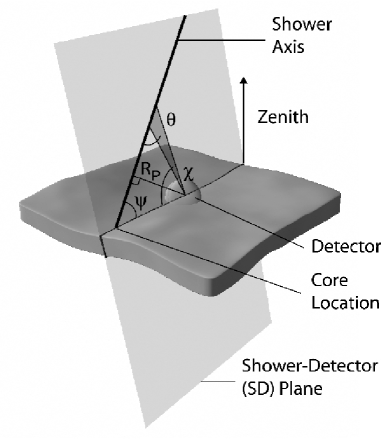
Figure 1: The geometry of reconstruction for a monocular air fluorescence detector

We can determine the plane of reconstruction very accurately. However, the value of $\psi$ is more difficult to determine accurately because it is dependent on the precise results of the profile-constrained fit [8, 10].

The HiRes-I angular resolution is therefore described by an elliptical, two-dimensional Gaussian distribution with the two Gaussian parameters, $\sigma_{\psi}$ and $\sigma_{\rm plane}$, being defined by the two angular resolutions. For the range of estimated energies considered in this paper, $\sigma_{\psi}=[4.9,6.1]^{\circ}$ and $\sigma_{\rm plane}[0.4,1.5]^{\circ}$. In figure 2,

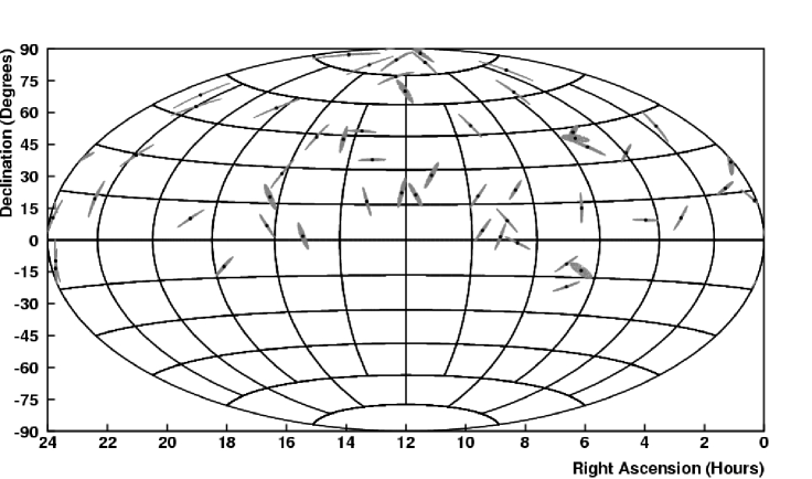
Figure 2: The arrival directions of the HiRes-I monocular with reconstructed energies above $10^{19.5}$ eV events and their $1\sigma$ angular resolution

the arrival directions of the HiRes-I events are plotted in equatorial coordinates along with their $1\sigma$ error ellipses.

In order to understand the systematic uncertainty in the angular resolution estimates, we consider a comparison of estimated arrival directions that successfully reconstructed in both HiRes-I monocular mode and HiRes stereo mode. Because of the dearth of events with estimated energies above $10^{19.5}$ eV that reconstructed satisfactorily in both stereo and mono mode, we consider all mono/stereo candidate events with estimated energies above $10^{18.5}$ eV. In stereo mode, the shower detector planes of the two detectors are intersected, thus the geometry is much more precisely known and the total angular resolution is of order $0.6^{\circ}$, a number that is largely correlated to $\sigma_{\rm plane}$ and thus is negligible when added in quadrature to the larger term, $\sigma_{\psi}$. This allows us to perform a comparison of the angular resolution estimated through simulations to the observed angular resolution values of actual data. In figure 3,

Figure 3: Arrival direction error comparison between real data (mono vs. stereo) and simulated data for events with estimated energies above $10^{18.5}$ eV. The solid line histogram corresponds to the arrival direction error distribution of the monocular reconstructed Monte Carlo simulated data. The crosses correspond to the arrival directions error distribution observed for actual data by comparing the arrival directions estimated by the monocular and stereo reconstructions. The solid line in the ratio component corresponds to the fit $y=ax+b$ where $a=0.000\pm 0.011$ and $b=0.98\pm 0.11$.

we show the distribution of angular errors for real and simulated data. The uncertainty in the slope of the ratio (figure 3b) leads to an 7.5% uncertainty in the angular resolution.

3 The Published AGASA Data

The AGASA data with energies above 40 EeV has been published up to the year 2000 [2] and all but one of these events used for this calculation has a measured energy greater than $4\times 10^{19}$ eV. The AGASA estimated angular errors [1] are shown in figure 4.

Figure 4: The AGASA angular resolution as a function of estimated energy [1]

The AGASA angular errors (figure 4) are fit to a two-component Gaussian distribution:

$$n=N_{\circ}(E_{\rm EeV})\biggr{[}0.33\Delta\theta e^{-(\Delta\theta)^{2}/2\sigma_{1}^{2}}+0.67\Delta\theta e^{-(\Delta\theta)^{2}/2\sigma_{2}^{2}}\biggr{]}$$ (1)

where $\sigma_{1}=6.52^{\circ}-2.16^{\circ}\log_{10}E_{\rm EeV}$, $\sigma_{2}=3.25^{\circ}-1.22^{\circ}\log_{10}E_{\rm EeV}$, and $N_{\circ}(E)$ is a numerically determined normalization constant. Figure 5

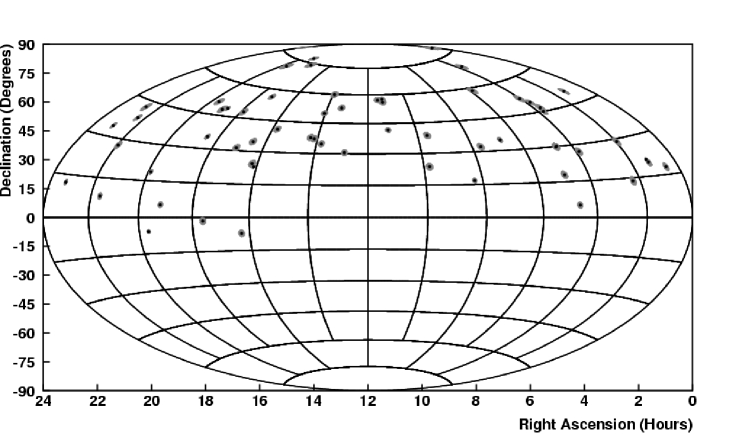
Figure 5: The arrival directions of the published AGASA events with their 68% angular resolution

shows the arrival directions of the published AGASA events plotted in equatorial coordinates with their 68% angular resolution.

4 The Autocorrelation Function

We measure the degree of autocorrelation in both samples by means of an autocorrelation function. It is calculated as follows:

1. For each event, an arrival direction is sampled on a probabilistic basis from the error space defined by the angular resolution of the event.

2. The opening angle is measured between the arrival directions of a pair of events.

3. The cosine of the opening angle is then histogrammed.

4. The preceding steps are repeated until all possible pairs of the events are considered.

5. The preceding steps are repeated until the error space, in the arrival direction of each event, is thoroughly sampled.

6. The histogram is normalized and the resulting curve is the autocorrelation function.

Figure 6a

(a)

(b)

Figure 6: An example of the autocorrelation function for a simulated data set that contains $\sim 10$ clusters in a total of 60 events—(a) the full autocorrelation function for $\theta=[0^{\circ},180^{\circ}]$; (b) the critical region of the the autocorrelation function: $\theta=[0^{\circ},10^{\circ}]$.

shows an example of the autocorrelation function for a highly clustered set of simulated data. The sharper the peak at $\cos\theta_{\rm min}$ is, the more highly autocorrelated the data set is. There are many ways that one could quantify the degree of autocorrelation that a set possesses. The most obvious way is to look at the value of the bin which contains $\cos\theta_{\rm min}$. However, this method has some pitfalls. First of all, the value of the last bin is dependent upon the chosen bin width. Also, the value of the last bin is not stable unless the angular resolution is sampled at a level that is computationally unfeasible. Finally, the value of the last bin over a large number of similarly autocorrelated sets does not produce a Gaussian distribution (see figure 7a),

(a)

(b)

Figure 7: Distributions of normalized bin densities of $\cos\theta_{\rm min}$ and $<\!\!\cos\theta\!\!>_{[0^{\circ},10^{\circ}]}$ values for a large number of simulated sets with the same level of clustering as in figure 6—(a) Distribution of observed normalized bin densities of $\cos\theta_{\rm min}$, note that it is not Gaussian ($\chi^{2}/dof=5.44$); (b) : $<\!\!\cos\theta\!\!>_{[0^{\circ},10^{\circ}]}$ distribution ($\chi^{2}/dof=1.09$).

thus complicating the interpretation of the results of an analysis employing $\cos\theta_{\rm min}$ as an observable.

A more well-behaved measure of the autocorrelation of a specific set of data is the value of $<\!\!\cos\theta\!\!>$ for $\theta\leq 10^{\circ}$. This value is also a measure of the sharpness of the autocorrelation peak at $\cos\theta=1$. However, this method of quantification does not depend on bin width and it does produce Gaussian distributions when it is applied to large numbers of sets with similar degrees of autocorrelation as is demonstrated in figure 7b. An additional advantage to this method is that by considering the continuous autocorrelation function over a specified interval, both the peak at the smallest values of $\theta$ and the corresponding statistical deficit in the autocorrelation function at slightly higher values of $\theta$ are taken into account. Thus we simultaneously measure both the positive and negative aspects of the autocorrelation signal. The interval of $[0^{\circ},10^{\circ}]$ was chosen because in simulations it was found to optimize the autocorrelation signal for clusters resulting from point sources spread isotropically across the sky.

Using the description of the HiRes-I monocular angular resolution above, we then calculate the autocorrelation function via the method described above. In figure 8,

(a)

(b)

Figure 8: The autocorrelation for the HiRes-I events above $10^{19.5}$ eV—(a) the full autocorrelation function for $\theta=[0^{\circ},180^{\circ}]$; (b) the critical region of the autocorrelation function: $<\!\!\cos\theta\!\!>_{[0^{\circ},10^{\circ}]}=0.99234$.

we show the result of this calculation. For this sample, we obtain $<\!\!\cos\theta\!\!>_{[0^{\circ},10^{\circ}]}=0.99234$.

We also calculate the autocorrelation function for the published AGASA events. We show the result in figure 9.

(a)

(b)

Figure 9: The autocorrelation for the published AGASA events—(a) the full autocorrelation function for $\theta=[0^{\circ},180^{\circ}]$; (b) the critical region of the autocorrelation function: $<\!\!\cos\theta\!\!>_{[0^{\circ},10^{\circ}]}=0.99352$.

For this sample, we obtain $<\!\!\cos\theta\!\!>_{[0^{\circ},10^{\circ}]}=0.99352$.

5 Quantifying the Relative Sensitivity of HiRes-I and AGASA to Autocorrelation

In order to quantify the relative sensitivity of the AGASA and HiRes-I data sets, we must first understand the exposures of both detectors. For HiRes-I, we assemble a library of approximately $8\times 10^{4}$ simulated events with energies above $10^{19.5}$ eV. We then pair each event with times during which the detector was operating. A mirror-by-mirror correction is applied where simulated events are rejected if the mirror(s) that would have observed the event in question was not operating at the time that event would have occurred. Once $10^{7}$ pairings of simulated events and times are assembled, a surface plot is created of the event density on a bin by bin basis. The value of each bin is then normalized so that the mean value of all the bins in the observable sky $\delta=[-30^{\circ},90^{\circ}]$ is 1. The resulting surface plot is shown in a Hammer-Aitoff projection in figure 10. We have previously shown that this method produced zenith angle, azimuthal angle, and sidereal time distributions that were consistent with that observed in the actual data [11].

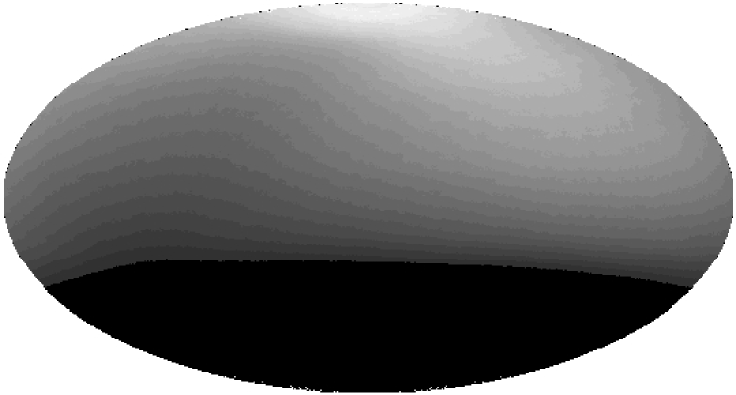
Figure 10: Hires-1 estimated relative exposure, $\rho_{\rm H}(\delta,\alpha)$, for events above $10^{19.5}$ eV in equatorial coordinates (right ascension right to left). The lightest region corresponds to a normalized event density of 2.5. The observable sky extends from $\delta=-30^{\circ}$ to $\delta=90^{\circ}$.

The highest exposure areas have a normalized relative exposure: $\rho_{\rm H}(\delta,\alpha)=\sim 2.5$.

For the AGASA detector, we refer to the distribution of event declinations presented in Uchiori et al. [13]. By following the lead of Evans et al. [14], we fit a normalized polynomial to this distribution:

$$N(\delta) = 0.323616+0.0361515\delta-5.04019\times 10^{-4}\delta^{2}+$$ (2)

$$5.539141\times 10^{-7}\delta^{3};$$

where $N(\delta)$ holds for $\delta=[-8^{\circ},87.5^{\circ}]$the maximum value of $N(\delta)$ is 1. We also know that:

$$A_{\circ}\int_{-8^{\circ}}^{87.5^{\circ}}N(\delta)\,d\delta=\int_{-8^{\circ}}^{87.5^{\circ}}\rho_{\rm A}(\delta)\cos\delta\,d\delta,$$ (3)

where $A_{\circ}$ is a numerically determined normalization constant. We then derive:

$$\rho_{\rm A}(\delta)=A_{\circ}N(\delta)\sec\delta;A_{\circ}=1.0251.$$ (4)

The value of each bin is once again normalized so that the mean value of all the bins in the observable sky $\delta=[-8^{\circ},87.5^{\circ}]$ is 1. The resulting surface plot is shown in a Hammer-Aitoff projection of a equatorial coordinates in figure 11.

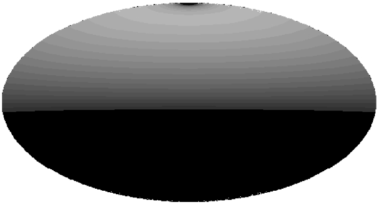
Figure 11: AGASA estimated relative exposure, $\rho_{\rm A}(\delta)$, for events above $10^{19.5}$ eV in equatorial coordinates (right ascension right to left). The lightest region corresponds to a normalized event density of $\sim 1.6$. The observable sky extends from $\delta=-8^{\circ}$ to $\delta=87.5^{\circ}$.

The highest exposure areas have $\rho_{\rm A}(\alpha)=\sim 1.6$. In figure 12,

(a)

(b)

Figure 12: Distribution of $<\!\!\cos\theta\!\!>_{[0^{\circ},10^{\circ}]}$ values for simulated isotropic data sets—(a) HiRes-I; (b) AGASA. In each figure, the vertical line represents the the value of $<\!\!\cos\theta\!\!>_{[0^{\circ},10^{\circ}]}$ for the observed data.

we show the distribution of $<\!\!\cos\theta\!\!>_{[0^{\circ},10^{\circ}]}$ values for isotropic data sets with each of the two different exposure models (HiRes-I and AGASA). The AGASA data set manifests $\sim 10^{-3}$ chance probability above background. For the AGASA data, we also calculated the autocorrelation function without consideration to angular resolution and employed the more conventional $\theta_{min}$ observable. After varying the bin width for $\theta_{min}$ and accounting for the trials factor, we independently concluded that the chance probability is $\sim 10^{-3}$ for the optimal bin width, $\theta_{min}=[0^{\circ},2.5^{\circ}]$. We thus conclude that factoring angular resolution into our analysis and employing $<\!\!\cos\theta\!\!>_{[0^{\circ},10^{\circ}]}$ as an observable in no way diminishes the sensitivity to autocorrelation in the reported AGASA data.

There are a few important differences between the exposure of the HiRes-I and AGASA detectors. First of all, the exposure of the HiRes-I detector is more asymmetric than the exposure of the AGASA detector. This is not only due to seasonal variations in the HiRes detector, but also due to its ability to constantly observe the region around $\delta=90^{\circ}$ due to a higher zenith angle acceptance. This higher zenith angle acceptance also allows the HiRes detector to observe a greater region of the southern hemisphere. In general, while AGASA reports observations for 56.9% of the total sky, the HiRes-I detector reports observations for 75% of the total sky.

To simulate clustering we use the following prescription:

1. An event is chosen based upon the distribution in $\alpha$ and $\delta$ that is dictated by $\rho$. In the case of HiRes-I, this is simply done by selecting a simulated event from our library and then assigning it a time that is a known good-weather ontime for the mirror(s) that observed that event. In the case of the AGASA detector, this is done by selecting a random value for $\delta$ that conforms to the distribution in equation (4) and then assigning it a random value in $\alpha$ between 0h and 24h and sampling a value for the energy from the energies of the reported events.

2. This event does not represent the source location itself, but is assumed to have arrived from the source location with some error. We construct a ”true” source location by sampling the error space of this event.

3. For each additional event assigned to that source, a simulated event is selected with a “true” arrival direction that is the same as that of the initial event.

To study the relative sensitivity of AGASA and HiRes-I, we measure the value of $<\!\!\cos\theta\!\!>_{[0^{\circ},10^{\circ}]}$ for multiple simulated sets with a variable number of doublets inserted. We then construct an interpolation of the mean value and standard deviation of $<\!\!\cos\theta\!\!>_{[0^{\circ},10^{\circ}]}$ from a given number of observed doublets for each experiment. This will allow us to state the number of doublets required for each experiment in order for the 90% confidence limit of $<\!\!\cos\theta\!\!>_{[0^{\circ},10^{\circ}]}$ to be above the background value of 0.99250. Figure 13

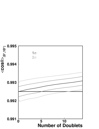
(a)	(b)
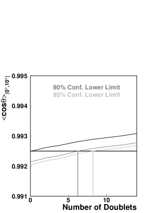
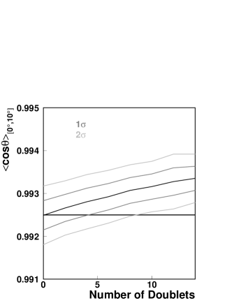
(c)	(d)

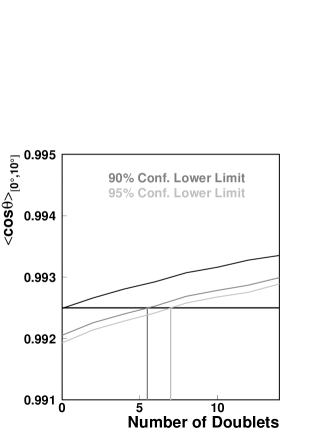
Figure 13: Relative sensitivity of HiRes-I and AGASA to doublets—(a) Simulations with the HiRes-I detector and 52 events; (b) 90% confidence above background: 6.25 doublets, 95% confidence above background: 8.25 doublets. (c) simulations with the AGASA detector and 59 events; (d) 90% confidence above background: 5.5 doublets, 95% confidence above background: 7.0 doublets. In each figure, the horizontal line indicates the expected value of $<\!\!\cos\theta\!\!>_{[0^{\circ},10^{\circ}]}$ for an isotropic background

shows the result of these simulations. In general, for the HiRes-I data set, the 90% confidence lower limit corresponds to the mean expected background signal with the inclusion of 6.25 doublets. For AGASA,the 90% confidence lower limit corresponds to the mean expected background signal with the inclusion of 5.5 doublets. This demonstrates that while AGASA has a slightly better ability to perceive autocorrelation, the sensitivity of the two experiments is comparable.

We now apply the actual Hires-I $<\!\!\cos\theta\!\!>_{[0^{\circ},10^{\circ}]}$ to the sensitivity curve shown in figure 13. In figure 14

(a)

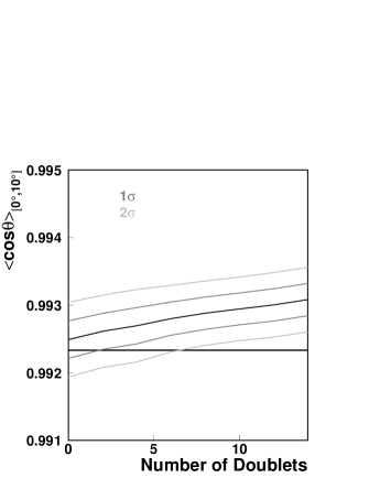
(b)

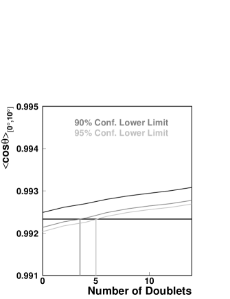
Figure 14: Sensitivity of the HiRes-I monocular observations to doublets—(a) Simulations with the HiRes-I detector and 52 events; (b) 90% confidence above observed signal: 3.5 doublets, 95% confidence above observed signal: 5 doublets. In each plot, the horizontal line represents the value of $<\!\!\cos\theta\!\!>_{[0^{\circ},10^{\circ}]}$ for the observed HiRes-I data

we can see the result of these simulations. The observed HiRes-I signal corresponds to the 90% confidence upper limit with the inclusion of only 3.5 doublets beyond random background coincidence.

If we repeat this analysis with first, a 7.5% reduction in the estimated angular resolution values and second, a 7.5% increase in the estimated angular resolution values, we obtain a range for the 90% confidence upper limit of $[2.75,4.0]$ doublets and a range for the 95% confidence upper limit of $[4.5,5.5]$ doublets.

A final area of concern is the systematic uncertainty in the determination of atmospheric clarity. Because hourly atmospheric observations are not available for the entire HiRes-I monocular data set, we have relied upon the use of an average atmospheric profile for the reconstruction of our data [12]. While different atmospheric conditions have negligible impact on the determination of the arrival direction for events with measured energies this high, differing conditions can have an impact on energy estimation and thus the number of events that are included in our data set. Over the $1\sigma$ error space for our estimation of atmospheric conditions, the total number of events in our data set fluctuates on the interval $[41,65]$. The value of the observable, $<\!\!\cos\theta\!\!>_{[0^{\circ},10^{\circ}]}$, has a fluctuation on the interval $[0.99226,0.99249]$ owing to addition and subtraction of events from the data set. Note that in neither case does the value of $<\!\!\cos\theta\!\!>_{[0^{\circ},10^{\circ}]}$ exceed the mean value (0.99250) expected for a background set.

6 Conclusion

We conclude that the HiRes-I monocular detector sees no evidence of clustering in its highest energy events. Furthermore, the HiRes-I monocular data has an intrinsic sensitivity to global autocorrelation such that we can claim at the 90% confidence level that there can be no more than 3.5 doublets above that which would be expected by background coincidence in the HiRes-I monocular data set above $10^{19.5}$ eV. From this result, we can then derive, with a 90% confidence level, that no more than 13% of the observed HiRes-I events could be sharing common arrival directions. This data set is comparable to the sensitivity of the reported AGASA data set if one assumes that there is indeed a 30% energy scale difference between the two experiments. It should be emphasized that this conclusion pertains only to point sources of the sort claimed by the AGASA collaboration. Furthermore, because a measure of autocorrelation makes no assumption of the underlying astrophysical mechanism that results in clustering phenomena, we cannot claim that the HiRes monocular analysis and the AGASA analysis are inconsistent beyond a specified confidence level.

7 Acknowledgments

This work is supported by US NSF grants PHY 9322298, PHY 9321949, PHY 9974537, PHY 0071069, PHY 0098826, PHY 0140688, PHY 0245428, PHY 0307098 by the DOE grant FG03-92ER40732, and by the Australian Research Council. We gratefully acknowledge the contributions from the technical staffs of our home institutions. We gratefully acknowledge the contributions from the University of Utah Center for High Performance Computing. The cooperation of Colonels E. Fisher and G. Harter, the US Army and the Dugway Proving Ground staff is appreciated.

References

- [1] M. Takeda et al., ApJ 522, 255 (1999) [arXiv:astro-ph/9902239].
- [2] M. Takeda et al., Proc. of 27th ICRC (Hamburg), 1, 337 (2001).
- [3] P. G. Tinyakov and I. I. Tkachev, JETP Lett. 74, 1 (2001) [Pisma Zh. Eksp. Teor. Fiz. 74, 3 (2001)] [arXiv:astro-ph/0102101].
- [4] C. B. Finley and S. Westerhoff, Accepted for publication in Astroparticle Physics [arXiv:astro-ph/0309159].
- [5] J. Bellido et al., Proc. of 27th ICRC (Hamburg), 1, 364 (2001).
- [6] J. Bellido et al., Proc. of 28th ICRC (Tsukuba), 1, 425 (2003).
- [7] R. U. Abbasi et al. [High Resolution Fly’s Eye Collaboration], Submitted for publication in Astrophysical Journal Letters [arXiv:astro-ph/0404137].
- [8] R. U. Abbasi et al. [High Resolution Fly’s Eye Collaboration], Phys. Rev. Lett. 92, 151101 (2004) [arXiv:astro-ph/0208243].
- [9] M. Takeda et al., Phys. Rev. Lett. 81, 1163 (1998) [arXiv:astro-ph/9807193].
- [10] T. Abu-Zayyad et al. [High Resolution Fly’s Eye Collaboration], Submitted for publication in Astroparticle Physics [arXiv:astro-ph/0208301].
- [11] R. Abbasi et al. [High Resolution Fly’s Eye Collaboration], Astropart. Phys. 21, 111 (2004) [arXiv:astro-ph/0309457].
- [12] L. R. Wiencke et al. [High Resolution Fly’s Eye Collaboration], Proc. of 27th ICRC (Hamburg), 1, 635 (2001).
- [13] Y. Uchihori, M. Nagano, M. Takeda, M. Teshima, J. Lloyd-Evans and A. A. Watson, Astropart. Phys. 13, 151 (2000) [arXiv:astro-ph/9908193].
- [14] N. W. Evans, F. Ferrer and S. Sarkar, Astropart. Phys. 17, 319 (2002) [arXiv:astro-ph/0103085].