The ESO-Sculptor Survey: Evolution of late-type galaxies at redshifts $0.1-0.5$

Using the Gaussian+Schechter composite luminosity functions measured from the ESO-Sculptor Survey (de Lapparent et al., 2003), and assuming that these functions do not evolve with redshift out to $z\sim 1$, we obtain evidence for evolution in the late spectral class containing late-type Spiral (Sc+Sd) and dwarf Irregular (dI) galaxies. There are indications that the Sc+Sd galaxies are the evolving population, but we cannot exclude that the dI galaxies also undergo some evolution. This evolution is detected as an increase of the Sc+Sd+Im galaxy density which can be modeled as either $n(z)\propto 1+3(z-0.15)$ or $n(z)\propto(1+z)^{2}$ using the currently favored cosmological parameters $\Omega_{m}=0.3$ and $\Omega_{\Lambda}=0.7$; the uncertainty in the linear and power-law evolution rates is of order of unity. For $\Omega_{m}=1.0$ and $\Omega_{\Lambda}=0.0$, the linear and power-law evolution rates are $\sim 4\pm 1$ and $\sim 2.5\pm 1$ respectively. Both models yield a good match to the ESS $BVR_{\mathrm{c}}$ redshift distributions to $21-22$^mag and to the number-counts to $23-23.5$^mag, which probe the galaxy distribution to redshifts $z\sim 0.5$ and $z\sim 1.0$ respectively.

The present analysis shows the usefulness of the joint use of the magnitude and redshift distributions for studying galaxy evolution. It also illustrates how Gaussian+Schechter composite luminosity functions provide more robust constraints on the evolution rate than pure Schechter luminosity functions, thus emphasizing the importance of performing realistic parameterizations of the luminosity functions for studying galaxy evolution.

The detected density evolution indicates that mergers could play a significant role in the evolution of late-type Spiral and dwarf Irregular galaxies. However, the ESO-Sculptor density increase with redshift could also be caused by a $\sim 1$^mag brightening of the Sc+Sd+dI galaxies at $z\sim 0.5$ and a $\sim 1.5-2.0$^mag brightening at $z\sim 1$, which is compatible with the expected passive brightening of Sc galaxies at these redshifts. Distinguishing between luminosity and density evolution is a major difficulty as these produce the same effect on the redshift and magnitude distributions. The detected evolution rate of the ESO-Sculptor Sc+Sd+dI galaxies is nevertheless among the range of measured values from the other existing analyses, whether they provide evidence for density or luminosity evolution.

1 Introduction

Since the availability of the deep optical numbers counts, the excess at faint magnitudes has provided the major evidence for galaxy evolution at increasing redshifts (Tyson, 1988; Lilly et al., 1991; Metcalfe et al., 1995). Using models of the spectro-photometric evolution of galaxies (Guiderdoni & Rocca-Volmerange, 1990; Bruzual & Charlot, 1993), either passive luminosity evolution or more complex effects have been suggested to explain the faint number-count excess (Guiderdoni & Rocca-Volmerange, 1991; Broadhurst et al., 1992; Metcalfe et al., 1995). Although the excess objects where initially envisioned as bright early-type galaxies at high redshift, the lack of a corresponding high redshift tail in the redshift distribution (Lilly, 1993) consolidated the interpretation in terms of evolution of later type galaxies, namely Spiral and/or Irregular/Peculiar galaxies (Campos & Shanks, 1997).

Here, we report on yet another evidence for evolution of the late-type galaxies, derived from the ESO-Sculptor Survey (ESS hereafter). The ESS provides a nearly complete redshift survey of galaxies at $z\la 0.5$ over a contiguous area of the sky. A reliable description of galaxy evolution require proper identification of the evolving galaxy populations and detailed knowledge of their luminosity functions. In this context, the ESS sample has the advantage to be split into 3 galaxy classes which are based on a template-free spectral classification (Galaz & de Lapparent, 1998), and which are dominated by the giant morphological types E+S0+Sa, Sb+Sc, and Sc+Sd+Sm respectively (de Lapparent et al., 2003, Paper I hereafter). In Paper I, we have performed a detailed measurement of the shape of the luminosity functions (LF hereafter) for the 3 ESS spectral classes. The spectral-type LFs show marked differences among the classes, which are common to the $B$, $V$, $R_{\mathrm{c}}$ bands, and thus indicate that they measure physical properties of the underlying galaxy populations.

The analysis of the ESS LFs in Paper I also provides a revival of the view advocated by Binggeli et al. (1988): a galaxy LF is the weighted sum of the intrinsic LFs for each morphological type contained in the considered galaxy sample; in this picture, differences in LFs mark variations in the galaxy mix rather than variations in the intrinsic LFs (Dressler, 1980; Postman & Geller, 1984; Binggeli et al., 1990; Ferguson & Sandage, 1991; Trentham & Hodgkin, 2002; Trentham & Tully, 2002). Local measures show that giant galaxies (Elliptical, Lenticular, and Spiral) have Gaussian LFs, which are thus bounded at both bright and faint magnitudes, with the Elliptical LF skewed towards faint magnitudes (Sandage et al., 1985; Jerjen & Tammann, 1997). In contrast, the LF for dwarf Spheroidal galaxies may be ever increasing at faint magnitudes to the limit of the existing surveys (Sandage et al., 1985; Ferguson & Sandage, 1991; Jerjen et al., 2000; Flint et al., 2001b, a; Conselice et al., 2002), whereas the LF for dwarf Irregular galaxies is flatter (Pritchet & van den Bergh, 1999) and may even be bounded at faint magnitudes (Ferguson & Sandage, 1989; Jerjen & Tammann, 1997; Jerjen et al., 2000). In Paper I, by fitting the ESS spectral-type LFs with composite functions based on the Gaussian and Schechter LFs measured for each morphological type in local galaxy groups and clusters (Sandage et al., 1985; Jerjen & Tammann, 1997), we confirm the morphological content in giant galaxies of the ESS classes, and we detect an additional contribution from dwarf Spheroidal (dE) and dwarf Irregular galaxies (dI) in the intermediate-type and late-type classes respectively. We then suggest that by providing a good match to the ESS spectral-type LFs, the local intrinsic LFs may extend to $z\sim 0.5$ with only small variations.

In the following, we report on the measurement of the amplitude of the LFs for the 3 ESS spectral-type LFs, and on the detection and measurement of redshift evolution for the late-type galaxies. Sect. 2 lists the main characteristics of the ESS spectroscopic survey. Sect. 3 recalls the definition of the ESS spectral classes and the technique for deriving the corresponding K-corrections and absolute magnitudes. Sect. 4 shows the measured composite fits of the ESS LFs for the 3 spectral classes. In Sect. 5, we describe the various techniques for measuring the amplitude of the LF (Sect. 5.1) and the associated errors (Sect. 5.2); we then apply these techniques to the ESS and show the detected evolution in the late-type galaxies (Sect. 5.3). In Sect. 6, we use the ESS magnitude number-counts to derive improved estimate of the late-type galaxy evolution rate in the $B$, $V$, and $R_{\mathrm{c}}$ bands. We then examine in Sect. 7 the redshift distributions for the 3 spectral classes in the 3 filters, and we verify that the measured evolution rates for the late-type galaxies match the ESS expected redshift distributions. Then, in Sect. 8, we compare the detected evolution in the ESS LF with those derived from other existing redshift surveys which detect either number density evolution (Sect. 8.1) or luminosity evolution (Sect. 8.2). Finally, Sect. 9 summarizes the results, discusses them in view of the other analyses which detect evolution in the late-type galaxies, and raises some of the prospects.

2 The ESS spectroscopic survey

The ESO-Sculptor Survey (ESS hereafter) provides a complete photometric and spectroscopic survey of galaxies in a region centered at $\sim 0^{\mathrm{h}}22^{\mathrm{m}}$ (R.A.) $\sim-30^{\circ}06^{\prime}$ (DEC.), near the Southern Galactic Pole. The photometric survey provides standard magnitudes $B$, $V$, and $R_{\mathrm{c}}$ in the Johnson-Cousins system, for nearly 13000 galaxies to $V\simeq 24$ over a contiguous rectangular area of $\sim 0.37$ deg² [$1.53^{\circ}\mathrm{(R{.}A{.})}\times 0.24^{\circ}\mathrm{(DEC{.})}$] (Arnouts et al., 1997). The uncertainties in the apparent magnitudes are $0.05$^mag in the $B$ $V$ and $R_{\mathrm{c}}$ bands for $R\mathrm{c}\la 21.0$ (Arnouts et al., 1997). Multi-slit spectroscopy of the $\sim 600$ galaxies with $R_{\mathrm{c}}\leq 20.5$ (Bellanger et al., 1995) have provided a 92% complete redshift survey over a contiguous sub-area of $\sim 0.25$ deg² [$1.02^{\circ}\mathrm{(R{.}A{.})}\times 0.24^{\circ}\mathrm{(DEC{.})}$]. Additional redshifts for $\sim 250$ galaxies with $20.5<R_{\mathrm{c}}\leq 21.5$ were also measured in the same sub-area, leading to a 52% redshift completeness to $R_{\mathrm{c}}\leq 21.5$ (see Paper I for details). We also consider here the $V\leq 21.0$ and $B\leq 22.0$ redshifts samples, which correspond to the combination of the $R_{\mathrm{c}}\leq 20.5$ “nominal” limit with the typical colors of galaxies at that limit: $B-R_{\mathrm{c}}\simeq 1.5$ and $V-R_{\mathrm{c}}\simeq 0.5$ (Arnouts et al., 1997)). The redshift completeness for the $V\leq 21.0$ and $B\leq 22.0$ samples is $91$% and $86$% respectively.

3 Spectral classification and K-corrections

Estimates of morphological types are not available for the ESS redshift survey. In Paper I, we estimate the ESS intrinsic LFs based on a spectral classification. Using a Principal Component Analysis, we have derived an objective spectral sequence, which is parameterized continuously using 2 parameters, describing respectively the relative fractions of old to young stellar populations (parameter denoted here $T_{\mathrm{S}}$), and the relative strength of the emission lines (Galaz & de Lapparent, 1998).

The ESS spectral sequence is separated into 3 classes, denoted “early-type”, “intermediate-type”, and “late-type”, which correspond to $T_{\mathrm{S}}\leq-5^{\circ}$, $-5^{\circ}<T_{\mathrm{S}}\leq 3^{\circ}$, and $T_{\mathrm{S}}>3^{\circ}$ respectively. These values separate the ESS spectroscopic $R_{\mathrm{c}}$, $V$, and $B$ samples into sub-samples with as least 100 galaxies (see Table 1). Given the moderate number of objects in the ESS spectroscopic sample, these 3 classes thus provide a satisfying compromise between resolution in spectral-type and signal-to-noise in the corresponding LFs.

Projection of the Kennicutt (1992) spectra onto the ESS spectral sequence shows that a tight correspondence with the Hubble morphological sequence of normal galaxies (Galaz & de Lapparent, 1998; Paper I); the ESS early-type class contains predominantly E, S0 and Sa galaxies, the intermediate-type class, Sb and Sc galaxies, and the late-type class, Sc, Sd and Sm/Im galaxies. We show that these spectral classes allow us to detect the respective contributions to the LF from the Elliptical, Lenticular and Spiral galaxies, and from the dwarf Spheroidal and Irregular galaxies.

In Paper I, we estimate the K-correction for the ESS by projecting templates extracted from the PEGASE spectrophotometric model of galaxy evolution onto the ESS spectral sequence. A fine mesh of model spectra with varying redshift and spectral-type are generated, and K-corrections in the $B$, $V$, and $R_{\mathrm{c}}$ filters are calculated for each of them; because the model spectra extend from 2000 Å to 10000 Å, we can derive K-corrections in the 3 bands up to $z\simeq 0.6$, the effective depth of the ESS redshift survey. A 2-D polynomial fit to the resulting surface in each filter provides analytical formulæ for the K-corrections as a function of redshift and spectral type, which are used for the ESS galaxies; these are plotted in Fig. 9 below, where they are compared with the K-corrections by Coleman et al. (1980, see Paper I for further details and comparisons). For each galaxy, the absolute magnitude $M$ is then derived from the apparent magnitude $m$, the spectral type $T_{\mathrm{S}}$ and the redshift $z$ using

$$M(m,z,T_{\mathrm{S}})=m-5\log d_{\mathrm{L}}(z)-K(z,T_{\mathrm{S}})-25,$$ (1)

where $d_{\mathrm{L}}(z)$ is the luminosity distance in Mpc (Weinberg, 1976):

$$d_{\mathrm{L}}(z)=(1+z)\;\frac{c}{H_{0}}\;\int_{0}^{z}[\;\Omega_{\mathrm{m}}(1+\upsilon)^{3}+\Omega_{\Lambda}\ ]^{-\frac{1}{2}}\;\mathrm{d}\upsilon\,$$ (2)

Throughout the present analysis, absolute magnitudes are calculated with a Hubble constant at present epoch written as $H_{0}=100h$ km s^-1 Mpc^-1. We also assume a flat Universe with values of the dimensionless matter density and cosmological constant assigned to $\Omega_{m}=0.3$, $\Omega_{\Lambda}=0.7$ resp., as currently favored (Riess et al., 1998; Perlmutter et al., 1999; Phillips et al., 2001; Tonry et al., 2003); when specified, $\Omega_{m}=1.0$ and $\Omega_{\Lambda}=0.0$ are also considered (see Sects. 4 and 6).

In Paper I, we report on all sources of random and systematic errors which affect the spectral classification, the K-corrections, and the absolute magnitudes. By comparison of the 228 pairs of independent spectra, we measure “external” errors in the K-corrections from 0.07 to 0.21 mag, and resulting uncertainties in the absolute magnitudes from 0.09 to 0.24^mag (with larger errors in bluer bands for both the K-corrections and the absolute magnitudes). From the 228 pairs of spectra, we also measure an “external” r.m.s. uncertainty in the redshifts of $\sigma\sim 0.00055$, which causes negligeable uncertainty in the absolute magnitudes compared to the other sources of error.

4 The shape of the ESS luminosity functions

Table 1: Parameters of the Gaussian and Schechter components of the composite luminosity functions fitted to the ESO-Sculptor spectral-type luminosity functions, in the $R_{\mathrm{c}}$, $V$, and $B$ filters.

Sample	Numb.	Morphol.	Gaussian component			Schechter component		$\phi_{0}$
	of gal.	content	$M_{0}-5\log h$	$\Sigma_{a}$	$\Sigma_{b}$	$M^{*}-5\log h$	$\alpha$	$\overline{0.4\ln 10\;\phi^{*}}$
early-type galaxies
$R_{\mathrm{c}}\leq 21.5$	291	E+S0+Sa	$-20.87\pm 0.23$	$0.84\pm 0.24$	$1.37\pm 0.36$
$V\leq 21.0$	156	E+S0+Sa	$-20.37$	$0.84$	$1.37$
$B\leq 22.0$	108	E+S0+Sa	$-19.47$	$0.84$	$1.37$
intermediate-type galaxies
$R_{\mathrm{c}}\leq 21.5$	270	Sb+Sc/dSph	$-20.27\pm 0.21$	$0.91\pm 0.18$		$-19.28\pm 0.37$	$-1.53\pm 0.33$	$0.83$
$V\leq 21.0$	169	Sb+Sc/dSph	$-19.87$	$0.91$		$-18.88$	$-1.53$	$0.83$
$B\leq 22.0$	154	Sb+Sc/dSph	$-19.27$	$0.91$		$-18.28$	$-1.53$	$0.83$
late-type galaxies
$R_{\mathrm{c}}\leq 21.5$	309	Sc+Sd/dI	$-19.16\pm 0.29$	$0.97\pm 0.13$		$-18.12\pm 0.22$	$-0.30$	$0.1$
$V\leq 21.0$	168	Sc+Sd/dI	$-18.76$	$0.97$		$-17.72$	$-0.30$	$0.1$
$B\leq 22.0$	190	Sc+Sd/dI	$-18.36$	$0.97$		$-17.32$	$-0.30$	$0.1$

• For the 2-component luminosity functions fitted to the intermediate-type and late-type galaxies, the morphological content of the 2 components appear separated by a “/”.

• The listed luminosity function parameters correspond to $H_{0}=100h$ km s^-1 Mpc^-1, $\Omega_{m}=0.3$, and $\Omega_{\Lambda}=0.7$.

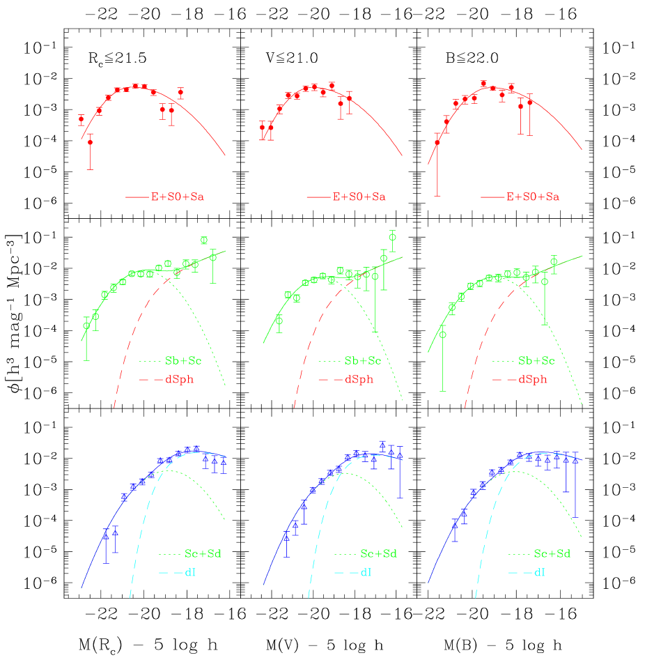
Figure 1: The ESO-Sculptor Gaussian+Schechter composite luminosity functions for the early-type (top panels), intermediate-type (middle panels), and late-type galaxies (bottom panels) in the 3 samples: $R_{\mathrm{c}}\leq 21.5$ (left panels), $V\leq 21.0$ (central panels) and $B\leq 22.0$ (right panels). Symbols indicate the SWML solution, and lines the composite fits obtained; all were obtained with $H_{0}=100h$ km s^-1 Mpc^-1, $\Omega_{m}=1.0$, and $\Omega_{\Lambda}=0.0$. The shape parameters of the composite functions converted to $\Omega_{m}=0.3$ and $\Omega_{\Lambda}=0.7$ are listed in Table 1.

The shape of the LFs for the 3 ESS spectral classes are derived in Paper I, using both the non-parametric step-wise maximum likelihood method (SWML) developed by Efstathiou et al. (1988), and the method of Sandage et al. (1979, denote STY) which assumes a specific parametric form for the LF. Although pure Schechter (1976) functions provide acceptable STY fits to the 3 ESS spectral-classes, we show that as good or better STY fits of the $R_{\mathrm{c}}$ LFs are obtained using composite functions based on the intrinsic LFs per morphological type measured in local groups and clusters (Jerjen & Tammann, 1997; Sandage et al., 1985).

For the ESS intermediate-type and late-type $R_{\mathrm{c}}$ LFs, we fit the sum of a Gaussian component representing the giant galaxies (Sb+Sc, and Sc+Sd resp.), and a Schechter component representing the dwarf galaxies (dSph and dI resp.). The Gaussian component is parameterized as

$$\phi(M)\;\mathrm{d}M=\phi_{0}e^{-(M_{0}-M)^{2}/2\Sigma^{2}}\;\mathrm{d}M,$$ (3)

where $M_{0}$ and $\Sigma$ are the peak and r.m.s. dispersion respectively. The Schechter (1976) component is parameterized as

$$\phi(L)\;\mathrm{d}L=\phi^{*}\left(\frac{L}{L^{*}}\right)^{\alpha}e^{-\frac{L}{L^{*}}}\;\mathrm{d}\left(\frac{L}{L^{*}}\right)$$ (4)

where $\phi^{*}$ is the the amplitude, $L^{*}$ the characteristic luminosity, and $\alpha$ determines the behavior at faint luminosities. Rewritten in terms of absolute magnitude, Eq.4 becomes:

$$\begin{array}[]{ll}\phi(M)\;\mathrm{d}M&=0.4\ln 10\;\phi^{*}e^{-X}X^{\alpha+1}\;\mathrm{d}M\\ {\rm with}&\\ X&\equiv\frac{L}{L^{*}}=10^{\;0.4\,(M^{*}-M)}\\ \end{array}$$ (5)

where $M^{*}$ is the characteristic magnitude, and $\alpha+1$ the “faint-end slope”.

For the ESS early-type $R_{\mathrm{c}}$ LF, a two-wing Gaussian function is used (a Gaussian with two different dispersion wings at the bright and faint end), as it successfully reflects the combination of a skewed LF towards faint magnitudes for the Elliptical galaxies with a Gaussian LF for the Lenticular galaxies displaced towards brighter magnitudes and with a narrower dispersion. The two-wing Gaussian is parameterized as

$$\begin{array}[]{ll}\phi(M)\;\mathrm{d}M&=\phi_{0}e^{-(M_{0}-M)^{2}/2\Sigma_{a}^{2}}\;\mathrm{d}M\;{\rm for}\;M\leq M_{0}\\ &=\phi_{0}e^{-(M_{0}-M)^{2}/2\Sigma_{b}^{2}}\;\mathrm{d}M\;{\rm for}\;M\geq M_{0}\\ \end{array}$$ (6)

where $M_{0}$ is the peak magnitude, and $\Sigma_{a}$ and $\Sigma_{b}$ are the dispersion values for the 2 wings. The improvement of the composite LFs over pure Schechter LFs is most marked for the early-type LF, because of its bounded behavior at faint magnitudes which is better adjusted by a Gaussian than a Schechter function, and for the late-type LF which cannot be fitted by a single Schechter function at simultaneously faint and intermediate magnitudes.

The ESS $R_{\mathrm{c}}$ LFs are measured for both the $R_{\mathrm{c}}\leq 20.5$ and $R_{\mathrm{c}}\leq 21.5$ samples in Paper I. Here we choose to use the LFs measured from the deeper sample because the faint-end of the LF is better defined than from the shallower sample. Composite fits to the LFs for the $V\leq 21.0$ and $B\leq 22.0$ samples have not been performed in Paper I. Here, we however need these fits in order to use the constraints on galaxy evolution provided by the $V$ and $B$ faint number counts. Instead of performing the STY composite fits in the $V$ and $B$ bands, which requires particular care because of the number of parameters involved, we prefer to use the simpler approach of converting the $R_{\mathrm{c}}$ LF parameters into the $V$ and $B$ bands. We showed in Paper I that the shift in magnitude of the $V$ and $B$ LFs with respect to the $R_{\mathrm{c}}$ is close to the mean $V-R_{\mathrm{c}}$, $B-R_{\mathrm{c}}$ resp. color of the galaxies in the considered spectral class. Moreover, the selection biases affecting the $V$ and $B$ samples (a deficiency in galaxies bluer than $B-R_{\mathrm{c}}\simeq 1.5$ and $V-R_{\mathrm{c}}\simeq 0.5$ resp., due to the selection of the spectroscopic sample in the $R_{\mathrm{c}}$ band) affect the faint-end of the late-type LF when fitted by pure Schechter functions, making it flatter than in the $R_{\mathrm{c}}$ band. Conversion of the composite $R_{\mathrm{c}}$ LF into the $B$ and $V$ bands allow us to circumvent the problem of incompleteness in the $B$ and $V$ bands.

Figure 1 plots the LFs for the 3 galaxy types in the $R_{\mathrm{c}}\leq 21.5$, $V\leq 21.0$ and $B\leq 22.0$ samples. The points represent the SWML solutions derived with $(\Omega_{m},\Omega_{\Lambda}$)=(1.0,0.0) in Paper I. For the $R_{\mathrm{c}}\leq 21.5$ sample (left panels), the curves show the composite fits derived in Paper I; note that for the late-type LF, we have adopted the intermediate slope $\alpha=-0.3$ (between the values $\alpha=-0.8$ and $\alpha=0.39$ measured from the $R_{\mathrm{c}}\leq 20.5$ and $R_{\mathrm{c}}\leq 21.5$ samples; a slope $\alpha\simeq-0.3$ is also measured for Sm/Im galaxies in the Virgo cluster (Jerjen & Tammann, 1997)). The parameters for the $V$ and $B$ composite LFs (middle and right panels resp. of Fig. 1) are then derived from those for the $R_{\mathrm{c}}\leq 21.5$ sample by applying the mean $M(V)-M(R_{\mathrm{c}})$ and $M(B)-M(R_{\mathrm{c}})$ colors for each spectral class (we use the $R_{\mathrm{c}}\leq 20.5$ sample for the color estimation, rather than the $R_{\mathrm{c}}\leq 21.5$ sample, as the completeness at magnitudes fainter $R_{\mathrm{c}}=20.5$ is biased in favor of red objects). The colors are those listed in Table 4 of Paper I: $M(V)-M(R_{\mathrm{c}})=0.5,0.4,0.4$ and $M(V)-M(R_{\mathrm{c}})=1.4,1.0,0.8$ for early-type, intermediate-type, and late-type galaxies respectively.

Note that the SWML points in Fig. 1 account for the incompleteness per apparent magnitude interval, as described by Zucca et al. (1994). For the SWML points, a bin size of $\Delta M=0.48$^mag is used in all filters (smaller or larger bin sizes within a factor 2 yield similar curves). As the amplitudes of the composite fits and the SWML solutions in the Fig. 1, are so far undetermined (they are measured later on in Sects. 5 and 6), we adopt the following: we use the same normalization of the SWML curves as used in Paper I (see Table 3), using the amplitude $\phi^{*}$ measured from the pure Schechter fits; then for each sample, the composite is adjusted by least-square fit to the SWML points (with the ratio $\phi_{0}/0.4\ln 10\;\phi^{*}$ between the Gaussian and Schechter component kept fixed to the values in Table 1).

Figure 1 shows that the composite LFs provide good adjustment to the SWML solutions for each of the 3 spectral classes in each filter. In particular, the simple color shift used to define the composite LFs in the $V$ and $B$ bands provides good adjustments to the SWML points in both bands, despite the color biases affecting the redshift completeness of these samples. Note that the composite spectral-type LFs derived from the $R_{\mathrm{c}}\leq 21.5$ sample provide satisfying adjustment to the SWML points for the $R_{\mathrm{c}}\leq 20.5$ spectral-type samples.

In Paper I, the LFs are measured for cosmological parameters $\Omega_{m}=1.0$ and $\Omega_{\Lambda}=0.0$. Because the faint number counts which we use below to constrain the ESS evolution rate are sensitive to the cosmological parameters, we have converted these values to $\Omega_{m}=0.3$ and $\Omega_{\Lambda}=0.7$, the currently favored parameters (Riess et al., 1998; Perlmutter et al., 1999; Phillips et al., 2001; Tonry et al., 2003). Again, rather than re-running the composite fits, we apply the empirical corrections derived by de Lapparent (2003), as follows. When changing from ($\Omega_{m},\Omega_{\Lambda}$)=(0.3,0.7) to ($\Omega_{m},\Omega_{\Lambda}$)=(1.0,0.0), the variation in absolute magnitude due to the change in luminosity distance is $\Delta M\simeq 0.3^{\mathrm{mag}}$ at $z\simeq 0.3$, the peak redshift of the ESS (see Figs. 13-15). This empirical correction is confirmed by the results from Fried et al. (2001) and Blanton et al. (2001), who calculate galaxy LFs in both cosmologies. de Lapparent (2003) also apply a correction to the Schechter parameter $\alpha$, with $\delta\alpha\sim\Delta M/3$, due to the strong correlation between the $M^{*}$ and $\alpha$ parameters in a Schechter parameterization. Here we neglect this correction, which would amount to $\delta\alpha\sim 0.1$ for a pure Schechter parameterization; this value is comparable or smaller than the 1-$\sigma$ uncertainty in the faint-end slope $\alpha$ of the Schechter component for the ESS intermediate-type and late-type LFs, and than the 1-$\sigma$ uncertainty in the dispersion $\Sigma_{a}$ and $\Sigma_{b}$ of the 2-wing Gaussian fitted to the ESS early-type LF (see Table 1).

Table 1 lists the resulting LF shape parameters for the Gaussian and Schechter components ($M_{0}$, $\Sigma_{a}$, $\Sigma_{b}$, $M^{*}$, $\alpha$; for a symmetric Gaussian, $\Sigma$ is listed in the $\Sigma_{a}$ column): conversion to ($\Omega_{m}$,$\Omega_{\Lambda}$)=(0.3,0.7) is obtained by shifting all values of $M_{0}$ and $M^{*}$ by $-0.3^{\mathrm{mag}}$. The last column of Table 1 lists the ratio of amplitude $\phi_{0}/0.4\ln 10\;\phi^{*}$ between the Gaussian and Schechter component derived from the composite fits to the $R_{\mathrm{c}}\leq 21.5$ sample in Paper I. We adopt the same values of this ratio for the $V$ and $B$ LFs.

5 The amplitude of the ESS luminosity functions

The amplitude of the LF is proportional to the mean density of galaxies brighter than some absolute magnitude threshold. It is therefore a useful indicator of the large-scale variations in the luminous component of the matter density in the Universe, and its possible evolution with redshift.

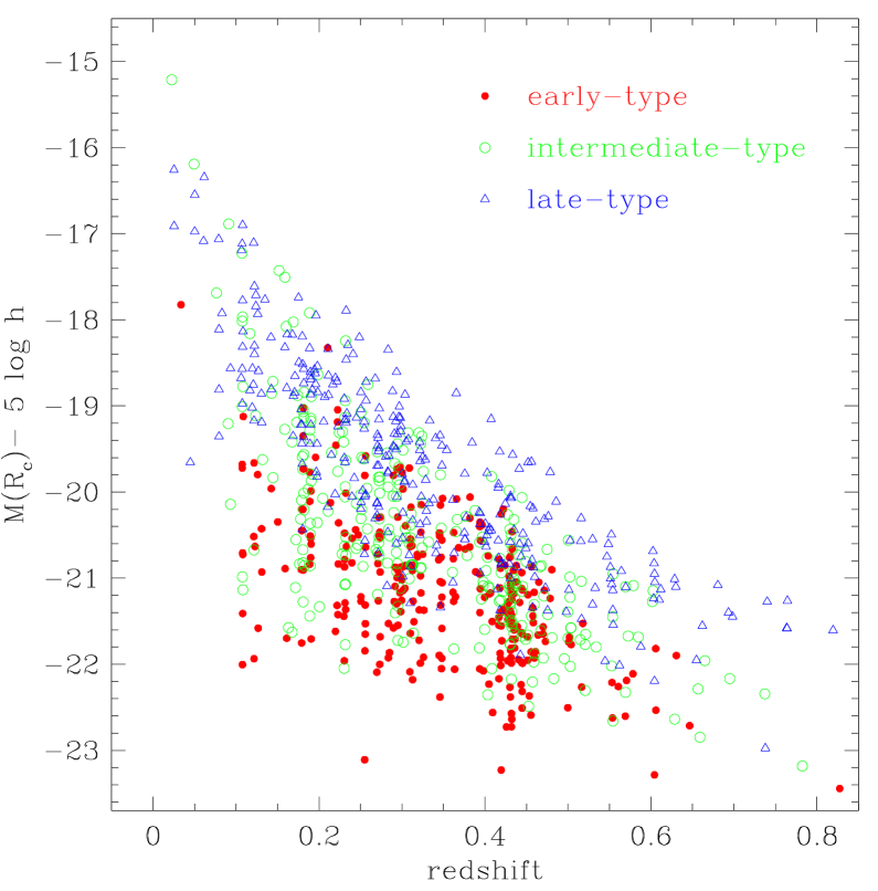
Figure 2: Absolute $R_{\mathrm{c}}$ magnitudes as a function of redshift $z$ for the ESS galaxies with $R_{\mathrm{c}}\leq 21.5$, using $H_{0}=100h$ km s^-1 Mpc^-1, $\Omega_{m}=0.3$, and $\Omega_{\Lambda}=0.7$. This graph shows how the apparent limiting magnitude biases the range of absolute magnitudes detected at increasing redshift, and how the varying K-corrections per spectral type affect the faintest absolute magnitude reached at a given redshift.

Several other redshift surveys probing the same redshift range as the ESS survey ($0.1\la z\la 0.5$) have detected signs of evolution in the intrinsic galaxy LFs (see Sect. 8 below). The major difficulty in measuring evolution of the LF with redshift originates from the limit in apparent magnitude which affects most redshift surveys. The flux limit results in the detection of galaxies in an absolute magnitude range which narrows with increasing redshift to the brightest galaxies. Figure 2 shows how the absolute magnitudes of the faintest detected ESS galaxies is a function of redshift and spectral-type (via the K-correction): the limiting curve at faint magnitudes is defined by replacing in Eq. 1 the apparent magnitude $m$ with the $R_{\mathrm{c}}=21.5$ magnitude limit, and the K-correction $K(T_{\mathrm{S}},z)$ with the smallest value over the considered spectral class at each $z$. Faint galaxies ($-18+5\log h\la M_{(}R_{\mathrm{c}})\la-15+5\log h$) are exclusively detected at $z\la 0.2$ in the ESS, whereas only bright early-type and intermediate-type galaxies with $M(R_{\mathrm{c}})\leq-21.0+5\log h$, and bright late-type galaxies with $M(R_{\mathrm{c}})\leq-20.0+5\log h$ are detected at $z\geq 0.5$. In the full ESS redshift range $0.1\la z\la 0.5$, only galaxies in the magnitude interval $-22.0+5\log h\la M_{R_{\mathrm{c}}}\la-21.0+5\log h$ can be observed, which is clearly too narrow for deriving any constraint on the evolution in the shape of the LF. Figures 3 and 4, which show the absolute $V$ and $B$ magnitudes versus redshift for the 3 spectral classes in the $V\leq 21.0$ and $B\leq 22.0$ samples resp., display similar effects. Driver (2001) showed that these biases strongly affect the usual tests for galaxy evolution based on the shape of the LF.

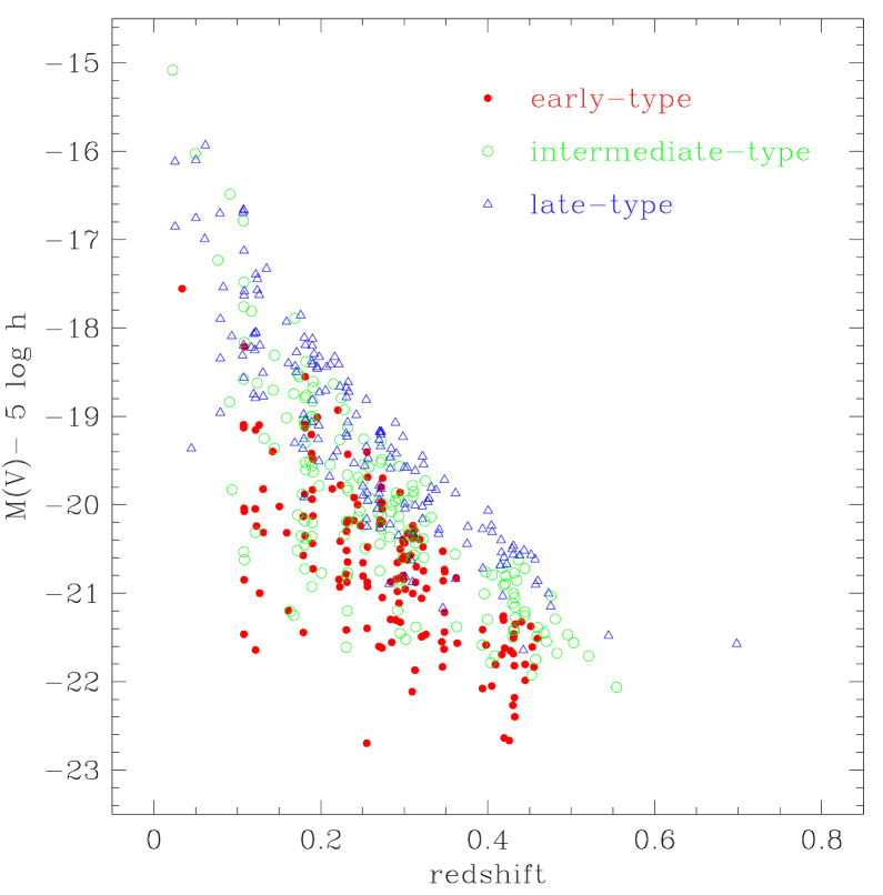
Figure 3: Same as Fig. 2 for $V\leq 21.0$.

The other limitation for detecting redshift evolution in the ESS is the limited statistics: separation of each of the 3 spectral classes into even as few as 2 redshifts intervals would yield large uncertainties in the measured shape of the LFs, which would make insignificant any reasonable difference between the high and low redshift LFs. For the ESS, we can only examine whether the “general” LF, i.e. the LF summed over all ESS spectral types, evolves with redshift. Here we consider the LF at $R_{\mathrm{c}}\leq 20.5$, as varying incompleteness at fainter magnitudes may act as evolution. For $(\Omega_{m},\Omega_{\Lambda})=(1.0,0.0)$, the ESS general LF for $R_{\mathrm{c}}\leq 20.5$ can be fitted by a Schechter function with $M^{*}=-20.95\pm 0.12+5\log h$ and $\alpha=-1.15\pm 0.09$ (STY fit). The corresponding LF in the redshift interval $z<0.3$ at $R_{\mathrm{c}}\leq 20.5$ has $M^{*}=-21.17\pm 0.21+5\log h$ and $\alpha=-1.18\pm 0.11$; at $z>0.3$, $M^{*}=-21.17\pm 0.28+5\log h$ and $\alpha=-1.63\pm 0.31$. The values of $M^{*}$ are identical in the 2 redshift ranges, and the slope $\alpha$ differs by 1.4-sigma; using ($\Omega_{m},\Omega_{\Lambda}$)=(0.3,0.7) yields similar conclusions. Given the difficulty in determining the parameter $\alpha$ in a Schechter fit (Paper I), these results are consistent with the hypothesis of null evolution in the shape of the ESS $R_{\mathrm{c}}$ “general” LF in the redshift range $0.1\la z\la 0.5$. This is however no proof that the individual spectral-type LFs do not vary in shape: one could imagine redshift variations in the shape of the intrinsic LFs which would conspire to combine into a constant “general” LF.

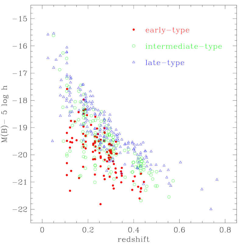
Figure 4: Same as Fig. 2 for $B\leq 22.0$.

Driver (2001) did suggest that reliable constraints on evolution of the shape of the galaxy LF at $z\la 1.25$ may only be derived from samples as deep as the Hubble Deep Field (Williams et al., 1996), which reaches $z\sim 3.5$ (Sawicki et al., 1997); Driver (2001) recommends that such analyses be rather based on the bi-variate brightness distribution for galaxies (the function which describes the galaxy bi-variate distribution in absolute magnitude and mean surface brightness). To circumvent the difficulty in measuring evolution in the shape of the LF, we assume in the following that the shape of the intrinsic LFs for the ESS early-type, intermediate-type, and late-type galaxies (as listed in Table 1) is not evolving with redshift. Any possible evolution will then be detected as evolution in the amplitude of the LF.

5.1 Measuring the amplitude of the luminosity function

Once the shape of the LF is determined, its amplitude can be determined in a second stage. We separate the amplitude $\Phi$ from the “shape” component $\varphi(M)\;\mathrm{d}M$:

$$\begin{array}[]{ll}\phi(M)\;\mathrm{d}M=&\Phi\;\varphi(M)\;\mathrm{d}M.\\ \end{array}$$ (7)

For a Gaussian LF, $\Phi=\phi_{0}$, and for a pure Schechter LF, $\Phi=0.4\ln 10\;\phi^{*}$ (see Eqs. 3 and 4). In a survey where the detected brightest and faintest absolute magnitudes are $M_{1}$ and $M_{2}$ resp., one can calculate the mean density of galaxies with $M_{1}\leq M\leq M_{2}$, denoted $\overline{n}\;(M_{1}\leq M\leq M_{2})$, which is related to $\Phi$ by

$$\Phi=\frac{\overline{n}\;(M_{1}\leq M\leq M_{2})}{\int_{M_{1}}^{M_{2}}\varphi(M)\;\mathrm{d}M};$$ (8)

In a magnitude-limited survey, the absolute magnitudes $M_{\mathrm{bright}}(z)$ and $M_{\mathrm{faint}}(z)$ of the detected brightest and faintest galaxy resp. vary with redshift (see Figs. 2-4). Calculation of the mean density $\overline{n}\;(M_{1}\leq M\leq M_{2})$ therefore requires to correct the observed number of galaxies to the expected number if the survey was limited to the constant absolute magnitude interval $M_{1}\leq M\leq M_{2}$. The correction is obtained by multiplying the observed number of galaxies at redshift $z$ by the inverse of the selection function $S(z)$ defined as

$$S(z)=\frac{\int_{\max(M_{\mathrm{bright}}(z),M_{1})}^{\min(M_{\mathrm{faint}}(z),M_{2})}\varphi(M)\;\mathrm{d}M}{\int_{M_{1}}^{M_{2}}\varphi(M)\;\mathrm{d}M};$$ (9)

For the ESS, we take in all filters $M_{1}=-30+5\log h$, and $M_{2}=-16+5\log h$ (see Figs. 2-4). $S(z)$ then measures the fraction of galaxies with $M_{1}\leq M\leq M_{2}$ at redshift $z$ which are included in the survey.

Following Davis & Huchra (1982), we define 3 estimators for the mean density $\overline{n}\;(M_{1}\leq M\leq M_{2})$ which are unbiased by the apparent magnitude limit of the survey (in the following, although we omit to mention $M_{1}\leq M\leq M_{2}$, all quoted densities refer to that interval). If $N(z)\;\mathrm{d}z$ is the observed number of galaxies in a shell $\mathrm{d}z$ at redshift $z$, $N(z)\;\mathrm{d}z/S(z)$ is the expected number of galaxies with $M_{1}\leq M\leq M_{2}$. A first estimator of the mean density is defined by Davis & Huchra (1982) as

$$n_{1}(z_{\mathrm{max}})=\frac{1}{V(z_{\mathrm{min}},z_{\mathrm{max}})}\int_{z_{\mathrm{min}}}^{z_{\mathrm{max}}}\frac{N(z)}{S(z)}\;\mathrm{d}z,$$ (10)

where $z_{\mathrm{min}}$ and $z_{\mathrm{max}}$ are arbitrary choices of the smallest and largest redshift over which the integrals are performed, and $V(z_{\mathrm{min}},z_{\mathrm{max}})$ is the total volume of the survey between these limits:

$$V(z_{\mathrm{min}},z_{\mathrm{max}})=\int_{z_{\mathrm{min}}}^{z_{\mathrm{max}}}\;\frac{\mathrm{d}V}{\mathrm{d}z}\;\mathrm{d}z$$ (11)

($\mathrm{d}V$ is the comoving volume element at redshift $z$, see Eq. 25). Here we use $z_{\mathrm{min}}=0.1$ (see Sect. 5.3). Note that because $1/S(z)$ rises sharply with redshift, the $n_{1}$ estimator heavily weights distant structures. Davis & Huchra (1982) also showed that $n_{1}$ is close to the minimum variance estimator of the mean density.

Davis & Huchra (1982) define another estimator by equating the observed number of galaxies with the expected number in a homogeneous universe:

$$n_{3}(z_{\mathrm{max}})=\frac{\int_{z_{\mathrm{min}}}^{z_{\mathrm{max}}}N(z)\;\mathrm{d}z}{\int_{z_{\mathrm{min}}}^{z_{\mathrm{max}}}S(z)\;\frac{\mathrm{d}V}{\mathrm{d}z}\;\mathrm{d}z}.$$ (12)

This estimator is much more stable than $n_{1}$, as all observed galaxies are weighted equally. It however heavily weights galaxies near the peak of the redshift distribution (Davis & Huchra, 1982).

Finally, Davis & Huchra (1982) define a third and intermediate estimator by averaging the expected density across radial shells:

$$n_{2}(z_{\mathrm{max}})=\frac{1}{z_{\mathrm{max}}-z_{\mathrm{min}}}\int_{z_{\mathrm{min}}}^{z_{\mathrm{max}}}\frac{N(z)}{S(z)\;\frac{\mathrm{d}V}{\mathrm{d}z}}\;\mathrm{d}z$$ (13)

The interest of the $n_{2}$ estimator is that its differential value

$$\mathrm{d}n_{2}=\frac{N(z)}{S(z)\;\frac{\mathrm{d}V}{\mathrm{d}z}}\;\mathrm{d}z$$ (14)

can also be calculated as a function of redshift, and allows one to examine the variations of the local galaxy density with redshift. Note that the 3 estimators $n_{1}$, $n_{2}$, and $n_{3}$ can be calculated to a varying depth $z_{\mathrm{max}}$ and are thus defined as functions of $z_{\mathrm{max}}$. In a fair sample of the galaxy distribution, that is a sample which is significantly larger than the largest density fluctuations, all 3 estimators should converge to a common value as $z_{\mathrm{max}}$ reaches the sample depth.

A fourth estimator, which we test here, is that proposed by Efstathiou et al. (1988). This estimator is similar to $n_{1}$ but the shell $\mathrm{d}z$ is taken to be infinitely small so that galaxies can be counted one by one, and the integral can be re-written as a sum over the galaxies in the sample:

$$n_{\mathrm{EEP}}(z_{\mathrm{max}})=\frac{1}{V(z_{\mathrm{min}},z_{\mathrm{max}})}\sum_{i=1}^{N_{\mathrm{gal}}}\frac{1}{S(z_{i})},$$ (15)

where $z_{i}$ is the redshift of each galaxy, $N_{\mathrm{gal}}$ galaxies are observed in the redshift range $z_{\mathrm{min}}-z_{\mathrm{max}}$, and the volume $V(z_{\mathrm{min}},z_{\mathrm{max}})$ is defined in Eq. 11.

The variations with $z_{\mathrm{max}}$ of the estimators $\Phi_{1}$, $\Phi_{2}$, $\Phi_{3}$, and $\Phi_{\mathrm{EEP}}$, based on $n_{1}(z_{\mathrm{max}})$, $n_{2}(z_{\mathrm{max}})$, $n_{3}(z_{\mathrm{max}})$, and $n_{\mathrm{EEP}}(z_{\mathrm{max}})$ respectively, can then be defined using Eq. 8. In practise, the integrals in the $n_{1}$, $n_{2}$ and $n_{3}$ estimators are calculated as discrete sums over a finite redshift bin $\Delta z$, and the selection function correction is approximated as $S(z_{\mathrm{c}})$ where $z_{\mathrm{c}}$ is the central redshift of the bin. However, because the second derivative of the selection function is positive, this yields an underestimate of the expected number of galaxies. The resulting systematic error in $\Phi$ is $\la 1$%. It is reduced to $\sim 0.1$% by replacing $S(z_{\mathrm{c}})$ by its average value over the bin, which we adopt for the $n1$, $n_{2}$ and $n_{3}$ estimators. The $n_{\mathrm{EEP}}$ estimator is a priori unbiased by this effect, as galaxies are considered one by one, and $S(z)$ is calculated at the redshift of each galaxy. Our tests with mock ESS catalogues (described in the next Sect.) however show that the $n_{\mathrm{EEP}}$ estimator tends to over-estimate the true $\Phi$ by $\sim 1$% for uniform distributions with $\sim 200$ points; this bias disappears for distributions with more than $\sim 2000$ points. In the ESS spectral classes for which $N_{\mathrm{gal}}\sim 100-300$ galaxies, a $\sim 1$% bias is small compared to the random uncertainties in the $n1$, $n_{2}$ and $n_{3}$ estimators (see next Sect.).

5.2 Estimation of errors

We estimate the random errors in the amplitude of the LFs for the ESS by generating mock ESS distributions with $\sim 240$, $\sim 2400$ and $\sim 24\,000$ points, and a Schechter LF defined by $M^{*}=-19.2$ and $\alpha=-1.4$ (using composite LFs as those listed in Table 1 would not change any of the reported results); the measured values of $\phi^{*}$ are then in proportion of the total number of galaxies in each simulation. The mock distributions have no built-in clustering, and are thus uniform spatial distributions modulated by the selection function (see Eq. 9). To nevertheless take into account the effects of large-scale clustering, we also introduce in the simulations density fluctuations in redshift which mimic large-scale structure: fluctuations resembling those measured in the ESS (measured as the departure from the redshift distribution for a uniform distribution), and various transformations of these including the inverse of the ESS fluctuations. We neglect density fluctuations transverse to the line-of-sight, as they are expected to have a negligeable effect on the calculation of the mean density.

For each type of simulation (choice of $\phi^{*}$ and fluctuations in density), we generate 100 samples with different seeds for the random generators. The random errors in the various estimators of $\phi^{*}$ are then calculated directly from the variance among the 100 realizations of the same distribution, and are functions of the redshift $z_{\mathrm{max}}$ out to which Eq. 10–13 are integrated. We measure that the variance in the estimator $\Phi_{3}$ of $\phi^{*}$ (based on $n_{3}$) varies as

$$\frac{\sigma(\Phi_{3})}{\Phi_{3}}\simeq\frac{1.0}{\sqrt{N_{\mathrm{gal}}(z_{\mathrm{min}},z_{\mathrm{max}})}}$$ (16)

where $N_{\mathrm{gal}}(z_{\mathrm{min}},z_{\mathrm{max}})$ is the number of galaxies in the survey which lie in the redshift interval $[z_{\mathrm{min}},z_{\mathrm{max}}]$. This is valid out to the most distant galaxy included in the survey. For the $n_{2}$ estimator of $\phi^{*}$, we measure

$$\frac{\sigma(\Phi_{2})}{\Phi_{2}}\simeq\frac{1.5}{\sqrt{N_{\mathrm{gal}}(z_{\mathrm{min}},z_{\mathrm{max}})}};$$ (17)

This is also valid out to the redshift where $N_{\mathrm{gal}}$ corresponds $\sim 95$% of the total number of galaxies in the sample ($z\simeq 0.6$ in the ESS). For the $n_{1}$ and $n_{\mathrm{EEP}}$ estimators, the relative variance in $\phi^{*}(z_{\mathrm{zmax}})$ rise slowly from $1.0/\sqrt{N_{\mathrm{gal}}(z_{\mathrm{min}},z_{\mathrm{max}})}$ at low redshift to $1.5/\sqrt{N_{\mathrm{gal}}(z_{\mathrm{min}},z_{\mathrm{max}})}$ when $N_{\mathrm{gal}}$ reaches $\sim 85$% of the total number of galaxies in the sample ($z\simeq 0.4$ in the ESS) and can grow to $2.0/\sqrt{N_{\mathrm{gal}}(z_{\mathrm{min}},z_{\mathrm{max}})}$ at larger distances (in the redshift interval $0.4<z<0.6$ for the ESS).

Davis & Huchra (1982) calculate that for the minimum variance estimate of the mean density (close to $n_{1}$), the relative uncertainty due to galaxy clustering within the finite volume sample is

$$\frac{\sigma(\overline{n})}{\overline{n}}\sim\sqrt{\frac{J_{3}(z_{\mathrm{min}},z_{\mathrm{max}})}{V(z_{\mathrm{min}},z_{\mathrm{max}})}},$$ (18)

where $4\pi J_{3}$ is the volume integral of the 2-point galaxy correlation in the survey volume bounded in redshift by $[z_{\mathrm{min}},z_{\mathrm{max}}]$. By using the correlation function $\xi(r_{\mathrm{P}},\pi)$ measured from the ESS by Slezak & de Lapparent (2004), we calculate the values of $J_{3}(z_{\mathrm{min}},z_{\mathrm{max}})$, and we confirm that the relative uncertainties derived from Eq. 18 for one spectral class are comparable to those given by Eq. 16 for $z_{\mathrm{min}}=0.1$ and $0.1\leq z_{\mathrm{max}}\leq 0.6$, with Eq. 18 becoming slightly larger than Eq. 16 at $z\la 0.3$.

As pointed by Lin et al. (1996), Eq. 18 and the errors calculated from the mock distributions underestimate the error in $\phi^{*}$, as they do not take into account the uncertainty in the shape of the LF: indeed, in our mock distributions, the LF is not re-measured, as we assume that the true value is known. In that case (when the input values of $M^{*}$ and $\alpha$ are used to calculate $\phi^{*}$), all 4 density estimators recover the true value to $0.1-1$% (see Eqs. 16 and 17). The systematic underestimation of $\phi^{*}$ by 20% calculated by Willmer (1997) for LFs derived by the STY estimator, could be a measure of this effect, if one assumes that $\phi^{*}$ was measured using the biased values of $M^{*}$ and $\alpha$ (but the author unfortunately does not specify). Here, however, we do not need to evaluate this additional source of uncertainty because the large amplitude of the density fluctuations on scales of 100 $h^{-1}$ Mpc  which are present in the ESS survey cause systematic variations in the determination of both $\phi^{*}$ and $\phi_{0}$ (see Sect. 5.3) which dominate all the other sources of error discussed here.

5.3 Evolution in the ESS mean density

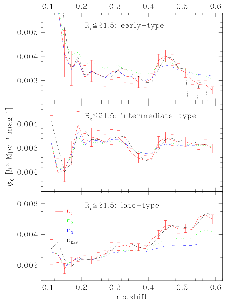
Figure 5: The amplitude $\phi_{0}$ of the Gaussian component of the composite luminosity functions measured for the ESO-Sculptor $R_{\mathrm{c}}\leq 21.5$ sample, using the estimators $n_{1}$ (red solid line), $n_{2}$ (green dotted line), $n_{3}$ (blue dashed line), and $n_{\mathrm{EEP}}$ (black dot-dashed line) defined in Eqs. 10–15, as a function of redshift (denoted $z_{\mathrm{max}}$ in the text). Each panel corresponds to a spectral-type. For clarity, only the random errors for the $n_{1}$ estimator, calculated using Eq. 16 are shown (see text for details). The error bars for the other curves have similar amplitude, except for $n_{2}$, for which they are 50% wider.

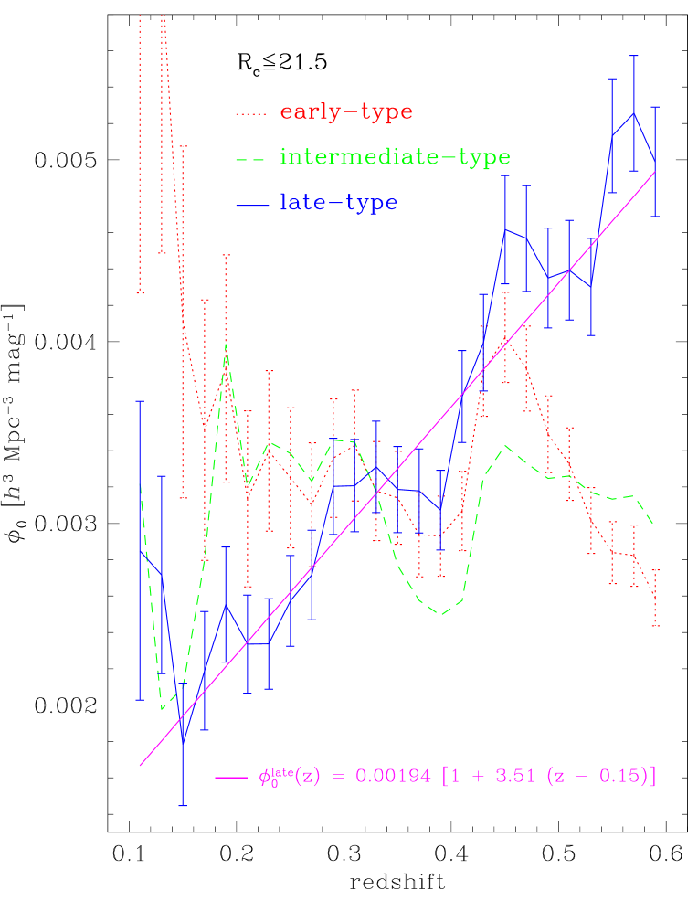
Figure 6: The amplitude $\phi_{0}$ of the Gaussian component of the composite luminosity functions measured for the ESO-Sculptor $R_{\mathrm{c}}\leq 21.5$ sample, using the estimator $n_{1}$ defined in Eq. 10, as a function of redshift $z_{\mathrm{max}}$; early-type, intermediate-type, late-type galaxies correspond to the red dotted, green dashed, and blue solid lines respectively. For clarity, the random errors for the intermediate-type galaxies are not shown; they are comparable to those for the early-type and late-type galaxies (see Eq. 16). The linear fit of Eq. 19 is also plotted (magenta solid straight line).

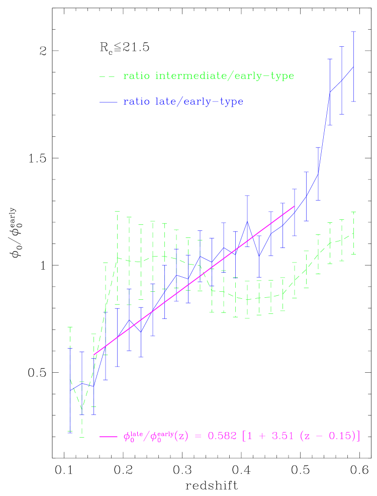
Figure 7: The amplitude $\phi_{0}(z_{\mathrm{max}})$ of the Gaussian component of the composite luminosity functions measured from the ESO-Sculptor $R_{\mathrm{c}}\leq 21.5$ sample for the intermediate-type (green dashed line) and late-type galaxies (blue solid line), both normalized to $\phi_{0}(z_{\mathrm{max}})$ for the early-type galaxies. All values of $\phi_{0}$ are derived using the $n_{1}$ estimator defined in Eq. 10. The linear fit to the relative late-type density given in Eq. 20 is also shown (magenta solid straight line).

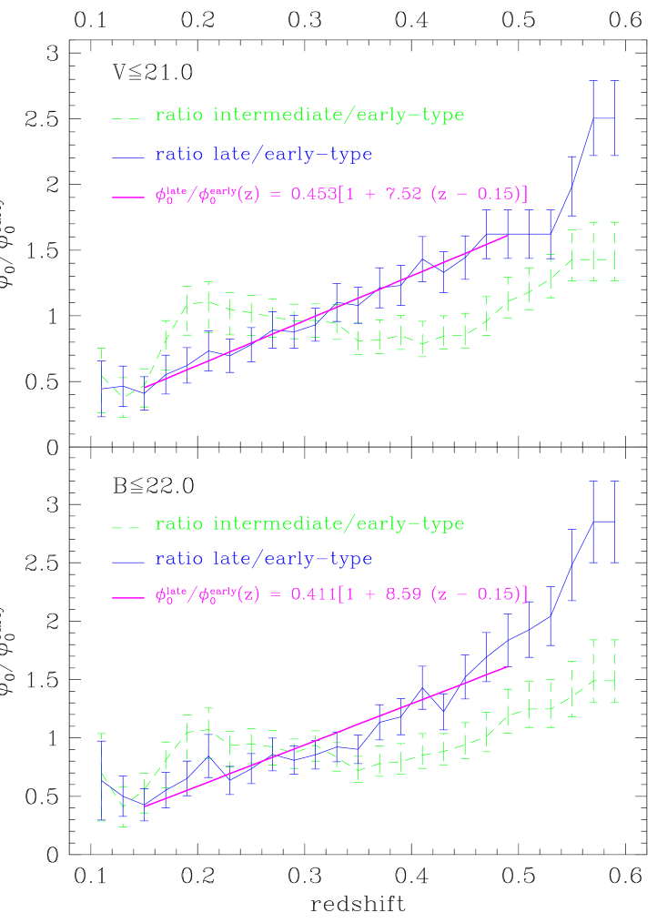
Figure 8: The amplitude $\phi_{0}(z_{\mathrm{max}})$ of the Gaussian component of the composite luminosity functions measured from the ESO-Sculptor $V\leq 21.0$ sample (top panel) and the $B\leq 22.0$ sample (bottom panel) for the intermediate-type (green dashed line) and late-type galaxies (blue solid line), both normalized to $\phi_{0}(z_{\mathrm{max}})$ for the early-type galaxies. All values of $\phi_{0}$ are derived using the $n_{1}$ estimator defined in Eq. 10. The linear fits to the relative late-type density and the corresponding parameterization are also shown in each panel (magenta solid straight line).

Figure 5 shows for each of the 3 ESS spectral classes the variations with redshift $z_{\mathrm{max}}$ of the estimates $\Phi_{1}$, $\Phi_{2}$, $\Phi_{3}$, and $\Phi_{\mathrm{EEP}}$ of the amplitude $\phi_{0}$ for the Gaussian component of the composite LFs (see Table 1 and Eqs. 3 and 6); these estimates are based on the $n_{1}(z_{\mathrm{max}})$, $n_{2}(z_{\mathrm{max}})$, $n_{3}(z_{\mathrm{max}})$, $n_{\mathrm{EEP}}(z_{\mathrm{max}})$ estimators of the mean density resp. (see Eqs. 10–15) for the ESS $R_{\mathrm{c}}\leq 21.5$ sample. All quantities plotted in Fig. 5 (and the other figures in this section) use $z_{\mathrm{min}}=0.1$, in order to avoid biasing of the density estimates, as the small volume probed at $z\leq 0.1$ suffers from under-sampling (see Figs. 2-4). The estimators $n_{1}$, $n_{2}$, $n_{3}$ are calculated in steps of $\Delta z=0.02$. The random errors due to the finite sample size for the $n_{1}$, $n_{3}$, and $n_{\mathrm{EEP}}$ estimators are evaluated using Eq. 16; for the $n_{2}$ estimator, Eq. 17 is used.

We emphasize that under the assumption of a non-evolving shape of the intrinsic LFs $\varphi(M)$ for the various galaxy types (see Sect. 5), examining the variations in $\phi_{0}$ with redshift is equivalent to examining the variations in the ESS mean density with redshift (see Eq. 8). Moreover, in the following, we only show and discuss the variations in the amplitude $\phi_{0}$ of the Gaussian component of each spectral-type LF. Nevertheless, because the variations in the amplitude $\phi^{*}$ of the Schechter components for the intermediate-type and late-type LFs are simply proportional to those in $\phi_{0}$ using the ratio $\phi_{0}/0.4\ln 10\,\phi^{*}$, whose values are listed in Table 1, all comments on the variations of $\phi_{0}$ also apply to those in $\phi^{*}$. In order to refer to both $\phi_{0}$ and $\phi^{*}$, we use in the following the generic amplitude $\Phi$.

We first compare the performances of the 4 estimators $n_{1}$, $n_{2}$, $n_{3}$ and $n_{\mathrm{EEP}}$. Figure 5 shows that the $n_{\mathrm{EEP}}$ estimator (Efstathiou et al., 1988) yields nearly indistinguishable results from the $n_{1}$ estimator. For all galaxy types, the $n_{3}$ estimator converges at $z\ga 0.5$ to a value determined by the ratio of total number of galaxies in the considered sample by the integral of $\varphi(M)$ (see Eq. 7); the asymptotic $n_{3}$ estimator of $\phi_{0}$ is however dominated by the observed number of galaxies at $z\la 0.3$ (see Sect. 5.1). In contrast, as the $n_{1}$ estimator weights different parts of the survey proportionally to their volume, it allows one to trace the large-scale density fluctuations across the ESS redshift interval. As expected, the $n_{2}$ estimator of $\phi_{0}$ (Eq. 13) yields intermediate values between the $n_{1}$ and $n_{3}$ estimators for the 3 galaxy types. In the following, we thus restrict the discussion to the extreme cases represented by the $n_{1}$ and $n_{3}$ estimators.

Figure 6 provides a direct comparison of the amplitude $\phi_{0}$ of the Gaussian component of the LFs based on the $n_{1}$ estimator (denoted $\phi_{1}$ hereafter) for the 3 ESS spectral types. The 3 curves show a relative depression in the range $0.33\la z\la 0.42$ followed by an excess at $z\sim 0.45$. Both features correspond to large-scale fluctuations in the redshift distribution. Note that for the 3 galaxy types, the fluctuations in the $\Phi_{1}$ about its mean value have a typical amplitude of $0.001$, corresponding to a relative variation of $\sim 30$%. These systematic errors largely dominate the random errors in $\Phi_{1}$ indicated by the vertical error-bars in Fig. 6 (see also Eqs. 16 and 17). The other marked effect in Fig. 6 is the steady increase of $\Phi_{1}$ for the late-type galaxies compared to the more stable behavior for the early-type and intermediate-type galaxies: a factor $\sim 2.5$ increase is measured from $z\simeq 0.15$ to $z\simeq 0.55$. We interpret this effect as an evolution in $\Phi_{1}$ for the late-type galaxies and provide further evidence below. An increase of $\Phi_{3}$ for the late-type galaxies is also visible in Fig. 5, but the effect is smaller as $\Phi_{3}$ applies a lower weight to the distant structures relative to those nearby.

Table 2: $n_{1}$ and $n_{3}$ estimators of the amplitude $\phi_{0}$ of the Gaussian component of the early-type, intermediate-type, and late-type luminosity functions for the ESO-Sculptor redshift survey, in the Johnson $B$, $V$ and Cousins $R_{\mathrm{c}}$ bands.

Sample	Early-type		Intermediate-type		Late-type
	$\Phi_{1}(0.51)$	$\Phi_{3}(0.51)$	$\Phi_{1}(0.51)$	$\Phi_{3}(0.51)$	$\Phi_{1}(z)$	$\Phi_{1}(0.51)$	$\Phi_{3}(0.51)$
$R_{\mathrm{c}}\leq 21.5$	$0.00333$	$0.00339$	$0.00326$	$0.00312$	$0.00194[1+3.51(z-0.15)]$	0.00439	0.00328
$R_{\mathrm{c}}\leq 20.5$	$0.00324$	$0.00331$	$0.00351$	$0.00321$	$0.00177[1+4.45(z-0.15)]$	$0.00462$	$0.00319$
$V\leq 21.0$	$0.00322$	$0.00335$	$0.00379$	$0.00314$	$0.00141[1+7.52(z-0.15)]$	$0.00521$	$0.00309$
$B\leq 22.0$	$0.00286$	$0.00363$	$0.00357$	$0.00325$	$0.00135[1+8.59(z-0.15)]$	$0.00551$	$0.00333$

• The listed values of the luminosity function amplitude $\phi_{0}$ are in units of  $h^{3}$ Mpc^-3 mag^-1, and are obtained with $H_{0}=100h$ km s^-1 Mpc^-1, $\Omega_{m}=0.3$, and $\Omega_{\Lambda}=0.7$.

• The corresponding amplitude $\phi^{*}$ of the Schechter component for the intermediate-type and late-type galaxies can be derived using the values of the ratio $\phi_{0}/0.4\ln 10\;\phi^{*}$ listed in Table 1.

• The $\Phi_{1}(z)$ parameterization of the evolving amplitude $\phi_{0}$ for the late-type galaxies should be used with caution (especially in the $V$ and $B$ bands); more realistic parameterizations are obtained in the $R_{\mathrm{c}}$, $V$ and $B$ bands from the adjustment of the number counts (see Table 4, Sect. 6).

The variations of $\Phi_{1}$ with redshift in Fig. 6 thus result from the combination of the density fluctuations produced by the pattern of large-scale structure with the possible evolution in the amplitude of the LF. A survey with a wider angular extent would be necessary to average out the effect of large-scale structures perpendicular to the line-of-sight. Although the different galaxy types have different clustering properties (Loveday et al., 1995), which on small scales are characterized by the morphology-density relationship (Dressler, 1980), they do trace the same pattern of walls and voids at large scales (Huchra et al., 1990). There has been so far no detection of systematic variations in the proportions of the different galaxy types on scales larger than $\sim 10$ $h^{-1}$ Mpc  (and thus outside galaxy clusters). We therefore make the hypothesis that the proportions of the different galaxy types are constant at large scales, and we eliminate the fluctuations caused by the large-scale structure by normalizing $\Phi_{1}$ for the intermediate and late-type galaxies by $\Phi_{1}$ for the early-type galaxies. The resulting relative variations of $\phi_{0}$ in the $R_{\mathrm{c}}\leq 21.5$ sample are shown in Fig. 7. The normalization erases most of the fluctuations in Fig. 6, and only the deviations from a distribution having similar large-scale clustering as the early-type galaxies remain. Whereas the relative density for the intermediate-type galaxies remains within the narrow interval $\sim 0.8-1.0$ in the redshift interval $0.15\la z\la 0.5$, the relative density of late-type galaxies shows a linear increase by a factor of nearly 2 in this interval.

Under the assumption that the shape $\varphi(M)$ of the intrinsic LFs for the various galaxy types are non-evolving with redshift (see Sect. 5), the systematic increase with redshift in the $\Phi_{1}$ estimate of $\phi_{0}$ for the late-type galaxies detected in Fig.7 can be interpreted as evidence for evolution in the ESS. A linear regression to the relative late-type density in the interval $0.15\leq z\leq 0.5$ yields

$$\frac{\phi_{0}^{\mathrm{late}}}{\phi_{0}^{\rm early}}(z)=0.582\;[1+3.51\,(z-0.15)];$$ (19)

this fit is over-plotted in Fig. 7. Note that the linear fit is performed in the restricted redshift interval $0.15\leq z\leq 0.5$ because the survey volume is too small at $z\leq 0.1$ (see Figs. 2-4) and the redshift survey is too diluted at $z\geq 0.5$ to provide a reliable estimate of $\phi_{0}$. We now assume that $\phi_{0}$ for the early-type galaxies does not evolve with redshift at $z\leq 0.5$, and that the redshift evolution in Eq. 19 can be fully attributed to the late-type galaxies. The parameterization of the late-type density evolution therefore becomes

$$\phi_{0}^{\mathrm{late}}(z)=\phi_{0}^{\mathrm{late}}(0.15)\;[1+P_{0.15}\,(z-0.15)]$$ (20)

with

$$\begin{array}[]{ll}P_{0.15}&=3.51\\ \phi_{0}^{\mathrm{late}}(0.15)&=0.00194\,h^{3}\,\mathrm{Mpc}^{-3}\,\mathrm{mag}^{-1}\\ \end{array}$$ (21)

The zero-point $\phi_{0}^{\mathrm{late}}(0.15)$ is measured by adjusting the linear fit to the measured values of the $\Phi_{1}$ estimate of $\phi_{0}$ at $z=0.51$ for the late-type galaxies, which is listed in Table 2. The linear evolution model of Eq. 20 is over-plotted in Fig. 6, with extrapolation to the redshift intervals $0.1\leq z\leq 0.15$ and $0.5\leq z\leq 0.6$. This model follows satisfactorily the increasing trend of the $\Phi_{1}$ estimator of $\phi_{0}$ for the late-type galaxies (recall that the deviations from the model are mostly caused by the large-scale structures).

We emphasize that the $\Phi_{1}(z)$ estimator at redshift $z$ is a cumulative measure over the redshift interval $0.1-z$, which may therefore underestimate the evolution rate for the late-type galaxies. However, the contribution at each redshift is proportional to the volume sampled; as the volume increases with $z^{2}$, this puts most of the weight on the structures at $z$, making $\Phi_{1}$ a good approximation to an incremental measure of the density variations with redshift. We also confirm this result by measuring the estimate of $\phi_{0}$ using the incremental estimator of the mean density $\mathrm{d}n_{2}$, described in Sect. 5.1 (Eq. 14). The estimator $\mathrm{d}n_{2}$ yields a similar rate of increase in $\phi_{0}$ as the $n_{1}$ estimator, but its large error bars prevent any reliable measure.

Other authors have modeled the evolution in the amplitude $\Phi$ of the LF as a power of $1+z$ (Lilly et al., 1996; Heyl et al., 1997), as it converts to a power of cosmic time for ($\Omega_{m}$,$\Omega_{\Lambda}$)=(1.0,0.0): $1+z\propto t^{-2/3}$ (Cole et al., 1992). Using the adopted values ($\Omega_{m}$,$\Omega_{\Lambda}$)=(0.3,0.7), adjustment of $\phi_{0}^{\rm late}/\phi_{0}^{\rm early}$ by a power-law function defined as

$$\phi_{0}^{\mathrm{late}}(z)=\phi_{0}^{\mathrm{late}}(0)\;(1+z)^{\gamma},$$ (22)

over the redshift interval $0.15\leq z\leq 0.5$, deviates from the linear model by at most $\sim 0.0001$ $h^{3}$ Mpc^-3 mag^-1, significantly smaller than the 1-$\sigma$ random errors in the measurement of $\phi_{0}^{\rm late}$ (see Fig. 6). Therefore, in the limited redshift range of the ESS, both the linear and power-law models provide good descriptions of the evolution of the relative density of late-type galaxies at $R_{\mathrm{c}}\leq 21.5$. In Sect. 6, we show that when extrapolated to $z\sim 1$, both the linear and power-law models can also adjust the ESS faint $BVR_{\mathrm{c}}$ number-counts.

For numerical comparison of the $\Phi_{1}$ and $\Phi_{3}$ estimators of $\phi_{0}$, we list in Table 2 their values at $z_{\mathrm{max}}=0.51$ for each spectral class of the $R_{\mathrm{c}}\leq 21.5$, $R_{\mathrm{c}}\leq 20.5$, $V\leq 21.0$ and $B\leq 22.0$ samples. For the early-type and intermediate-type galaxies, the values of $\Phi_{3}(0.51)$ show a systematic difference of $0.00006-0.0008$ $h^{3}$ Mpc^-3 mag^-1 with the corresponding values of $\Phi_{1}(0.51)$, due to the different weighting of the large-scale structure by the 2 estimators (see Sect. 5.1). In contrast, for the late-type galaxies, $\Phi_{3}(0.51)$ is systematically lower than $\Phi_{1}(0.51)$ by $\sim 0.001$ $h^{3}$ Mpc^-3 mag^-1  in $R_{\mathrm{c}}$ to $\sim 0.002$ $h^{3}$ Mpc^-3 mag^-1  in $V$ and $B$. Ignoring the evolution in the late-type density and using the $\Phi_{3}$ estimator of $\phi_{0}$ rather than $\Phi_{1}$ would then underestimate $\phi_{0}$ at $z\sim 0.5$ by $\sim 40-50$% in $R_{\mathrm{c}}$, and by $\sim 70$% in $V$ and $B$.

For the late-type galaxies, we also list in Table 2 the linear parameterization of $\Phi_{1}(z)$ (Eqs. 20 and 21). Comparison of the “zero-point” of the linear parameterization $\Phi_{1}(0.15)$ with the listed value of $\Phi_{1}(0.51)$ illustrates the increase in $\Phi_{1}$ from $z\sim 0.15$ to $z\sim 0.51$. Note that Table 2 also lists the parameters derived from the shallower but more complete $R_{\mathrm{c}}\leq 20.5$ sample (using the same LFs as for the $R_{\mathrm{c}}\leq 21.5$ sample, see Table 1). The evolution rate $P_{0.15}=4.45$ is close to that for the deeper $R_{\mathrm{c}}$ sample, and the values of $\Phi_{1}$ and $\Phi_{3}$ differ from those from the $R_{\mathrm{c}}\leq 21.5$ sample by less than 1-$\sigma$ (the uncertainties in $\Phi_{1}$ and $\Phi_{3}$ for all considered samples in Table 2 are in the interval $\sim 0.0002-0.0003$ for $z_{\mathrm{max}}\geq 0.3$).

We apply a similar analysis to the ESS $V\leq 21.0$ and $B\leq 22.0$ samples. The measured and modeled relative $\Phi_{1}$ estimators of $\phi_{0}$ are plotted in Fig. 8; the relative $\Phi_{1}$ for the intermediate-type galaxies are also plotted in Fig. 8. As in the $R_{\mathrm{c}}$ filter, the fits are performed in the restricted redshift interval $0.15\leq z\leq 0.5$. In both the $V$ and $B$ bands, we find an increase of the late-type galaxy density which confirms the reality of the effect detected in the $R_{\mathrm{c}}$ band. We however measure a factor of 2 higher evolution rate $P_{0.15}$ in $V$ and $B$ than in $R_{\mathrm{c}}$ (see Table 2). This may be due to the fact that when going to bluer bands, the late-type galaxies are favored. The higher evolution rate in the $V$ and $B$ bands may also reflect the color-dependent selection effects affecting the redshift samples in the $V$ and $B$ bands. Moreover, the variations in $P_{0.15}$ from band to band are symptomatic of the limited constraints provided by the ESS redshift distributions. In the following, we show that measuring the evolutions rates from the ESS faint magnitude number counts yields better agreement among the 3 filters.

6 Modeling the ESS number-counts

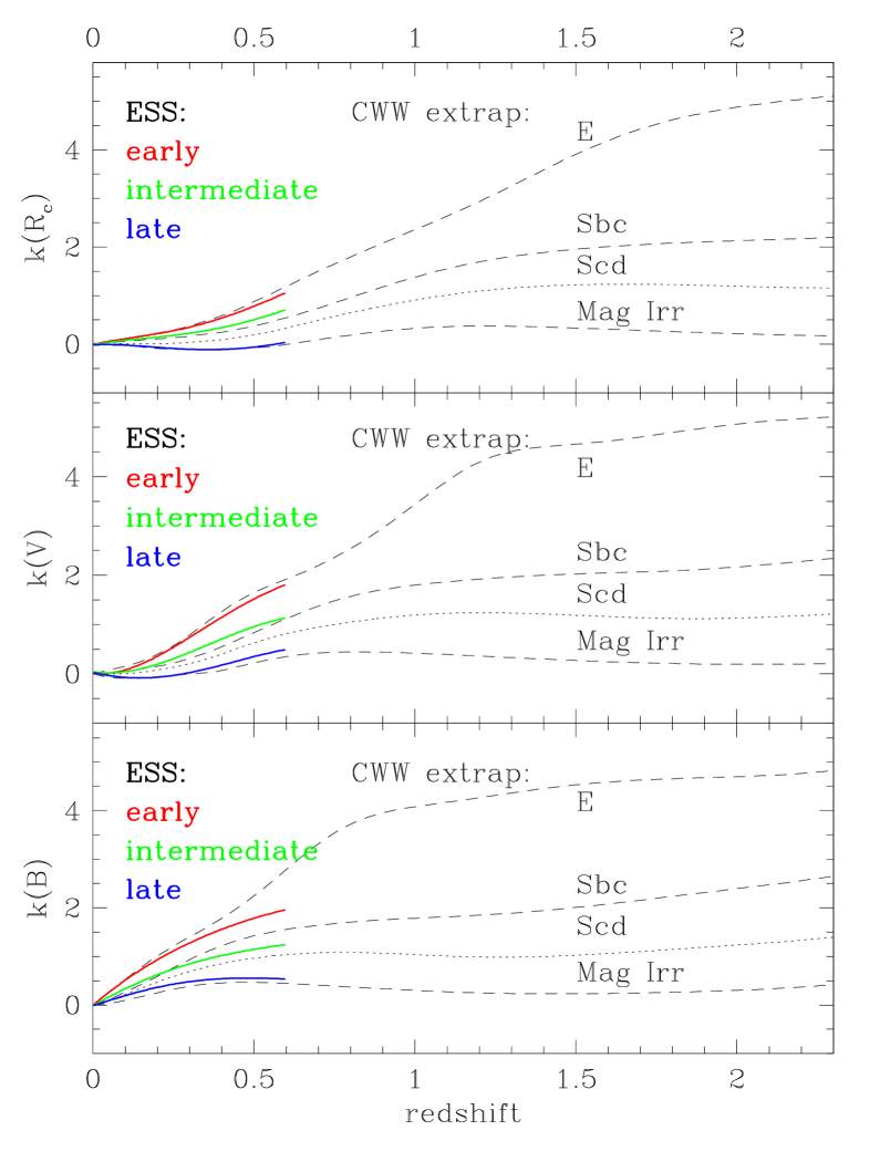
Figure 9: K-corrections in the $R_{\mathrm{c}}$ bands (top panel), $V$ (middle panel), and $B$ (bottom panel) derived from Coleman et al. (1980, labeled “CWW extrap” in graph; see text for details) which are used for predicting the ESO-Sculptor galaxy number counts in Figs. 10, 11 and 12: Elliptical, Sbc and Magellanic Irregular types are plotted as dashed lines (running from top to bottom), and are used to model the ESO-Sculptor K-corrections for the early-type, intermediate-type, and late-type galaxies respectively; K-corrections for “CWW extrap” type Scd are shown as dotted lines, for comparison. The polynomial K-corrections calculated for the 3 ESO-Sculptor spectral classes and valid only for $z<0.6$ are shown as heavy solid lines, with early-type, intermediate-type and late-type galaxies plotted from top to bottom.

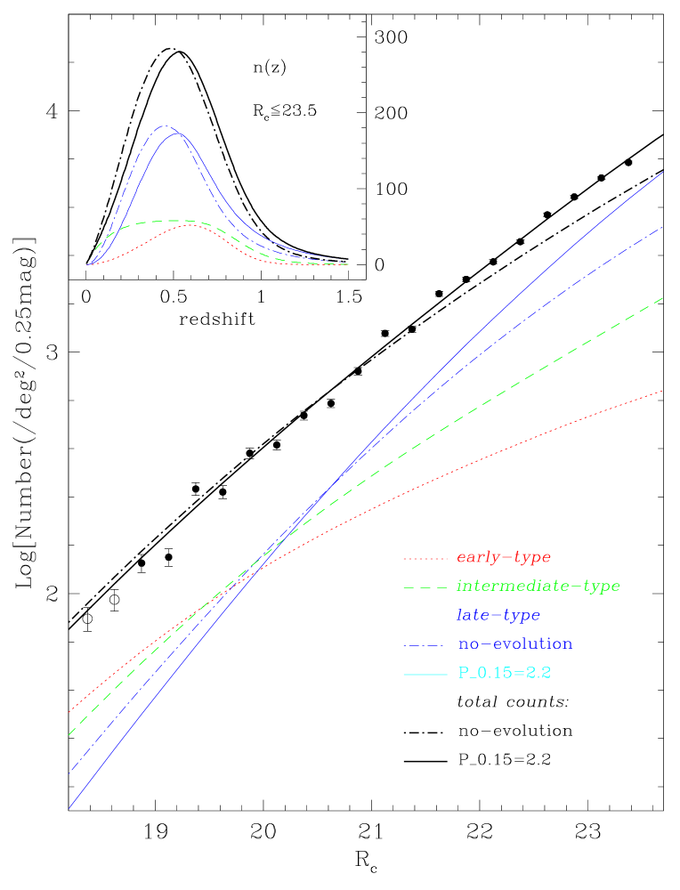
Figure 10: Comparison of the ESO-Sculptor magnitude number-counts in the $R_{\mathrm{c}}$ band per 0.25^mag interval (open and filled circles) with the modeled counts defined as the sum of the predicted number counts for the 3 considered spectral classes: early-type (red dotted line), intermediate-type (green dashed line), late-type with no-evolution (blue dot-dashed line), late-type with the best-fit evolution rate (blue solid line). The Gaussian+Schechter composite luminosity functions listed in Table 1 are used for the 3 classes. The amplitude $\phi_{0}$ of the Gaussian component of the luminosity function used for each galaxy class is identical to that used in Fig. 13. The black heavy dot-dashed line show the predicted total counts with no-evolution, and the black heavy solid line the adjusted total counts with evolution in the late-type galaxies (see text for details). Only the data points with more than 100 galaxies per bin (filled circles) are used for the adjustment of the total evolving counts. The plotted error bars in the observed counts are estimated as $\sqrt{n}$. The inset shows the predicted redshift distributions for the 3 spectral classes, with the same line coding as for the number-counts.

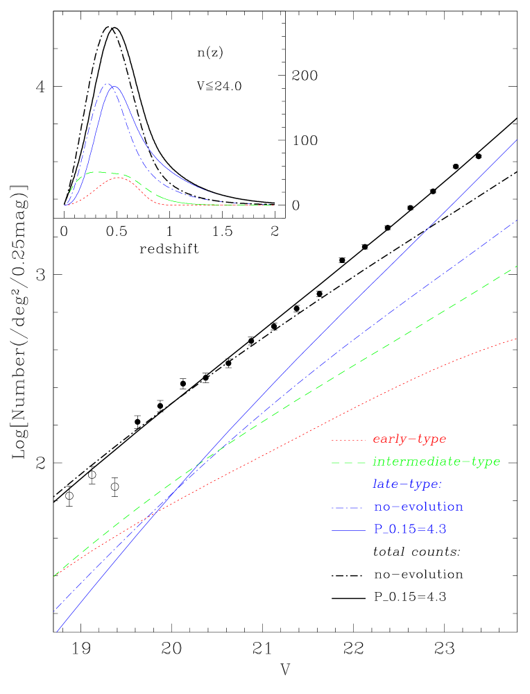
Figure 11: Same as Fig. 10 for the ESS number-counts per 0.25 mag interval in the $V$ band. The amplitude $\phi_{0}$ of the Gaussian component of the luminosity function used for each galaxy class is identical to that used in Fig. 14.

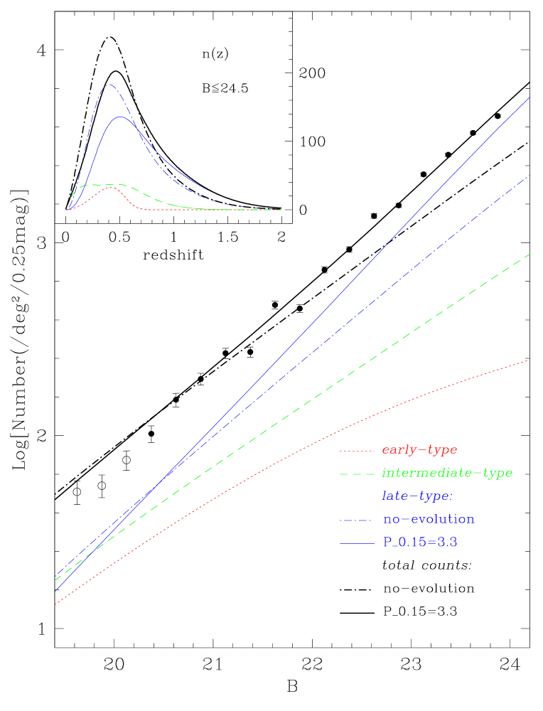
Figure 12: Same as Fig. 10 for the ESS number-counts per 0.25 mag interval in the $B$ band. The amplitude $\phi_{0}$ of the Gaussian component of the luminosity function used for each galaxy class is is identical to that used in Fig. 15.

Because the ESS number-counts extend nearly 3 magnitudes fainter than the spectroscopic catalogue, comparison of the observed galaxy counts with those predicted by the LFs provides a test of how well the measured LFs and evolution rates can be extrapolated from $z\simeq 0.5$ to $z\simeq 1$.

Figures 10, 11, 12 show the observed number counts in the $R_{\mathrm{c}}$, $V$ and $B$ bands resp., binned in intervals of 0.25^mag (Arnouts et al., 1997). In each band, the magnitude of the faintest plotted point corresponds to the completeness limit: $R_{\mathrm{c}}\simeq 23.5$, $V\simeq 23.5$, and $B\simeq 24$, respectively. At bright magnitudes, the plotted number count distributions start in the first 0.25^mag bin where the count is larger or equal to 50 galaxies, as the counts are highly uncertain at low count level. For the same reason, the fits described in the following start in the first bin where the count is larger or equal to 100, that is in the bins centered at $R_{\mathrm{c}}=18.875$, $V=19.625$ and $B=20.325$, respectively.

For modeling the galaxy number-counts, one must define a set of K-corrections. We cannot use the ESS polynomials K-corrections described in Sect. 3, as these are unconstrained at $z>0.6$, whereas the number-counts to magnitudes $\sim 24$ are produced by galaxies out to $z\sim 1.5$. In replacement, we use the K-corrections obtained from the optical spectra of Coleman et al. (1980), which have been extrapolated in the UV and the IR by using the theoretical SEDs of the GISSEL library (Charlot et al., 1996) for the 4 types Elliptical, Sbc, Scd, and Magellanic Irregular (see Sawicki et al., 1997; Arnouts et al., 1999). These K-corrections are shown in Fig. 9 for the $B$, $V$ and $R_{\mathrm{c}}$ bands (labeled “CWW extrap”). We choose to use for the ESS early-type, intermediate-type, and late-type, the K-corrections for the Elliptical, Sbc, and Magellanic Irregular types respectively. This choice is motivated by the comparison for $z\leq 0.6$ of the “CWW extrap” K-corrections with the ESS K-corrections for the 3 spectral classes, also shown in Fig. 9. In the common redshift interval, the 2 sets of K-corrections are in good agreement, with the largest deviations occurring in the $B$ band ($\sim 0.8$^mag for the early-type, $\simeq 0.3$^mag for the intermediate type, and $\simeq 0.1$^mag for the late-type galaxies), as it is the most sensitive band to the template shape in the UV at the redshifts considered here. The consistent evolution rates obtained in the following from the number-counts in the $R_{\mathrm{c}}$, $V$ and $B$ bands a posteriori indicates that the CWW-extrap K-corrections do not introduce any severe systematic effects in the modeled number-counts.

We then model the expected number-counts in each band as the sum of the predicted number-counts over the 3 galaxy spectral classes $T_{\mathrm{S}}$:

$$N(m)=\Sigma_{T_{\mathrm{S}}=1}^{3}N_{T_{\mathrm{S}}}(m),\\$$ (23)

where $m$ is the apparent magnitude in either of the $R_{\mathrm{c}}$, $V$ or $B$ filters. For each class, the expected number count $N_{T_{\mathrm{S}}}(m)$ is obtained by integrating the corresponding composite LF $\Phi_{T_{\mathrm{S}}}(M)$ (listed in Table 1) over all redshifts $0\leq z\leq z_{\mathrm{high}}$ contributing to absolute magnitude $M(m,z,T_{\mathrm{S}})$ at a fixed value of $m$ (see Eq. 1):

$$N_{T_{\mathrm{S}}}(m)=\int_{0}^{z_{\mathrm{high}}}\Phi_{T_{\mathrm{S}}}[M(m,z,T_{\mathrm{S}})]\;\frac{\mathrm{d}V}{\mathrm{d}z}\;\mathrm{d}z;\\$$ (24)

$\frac{\mathrm{d}V}{\mathrm{d}z}$ is the comoving volume element per unit solid angle defined as

$$\frac{\mathrm{d}V}{\mathrm{d}z}=\frac{c}{H_{0}}\;\frac{d_{\mathrm{L}}(z)^{2}}{(1+z)^{2}}\;\frac{1}{\sqrt{\Omega_{\mathrm{m}}(1+z)^{3}+\Omega_{\Lambda}}}.$$ (25)

The values of $z_{\mathrm{high}}$ are $1.5$ in the $R_{\mathrm{c}}$ band, and $2.0$ in the $B$ and $V$ bands. Note that $N(m)$ and $N_{T_{\mathrm{S}}}(m)$ in Eqs. 23 and 24 resp.  are defined as number counts per unit solid angle and per unit magnitude interval. The curves plotted in Figs. 13 to 15 are then multiplied by 0.25^mag and $\pi^{2}/180^{2}$ (to convert to number counts per 0.25^mag interval per square degree).

Table 3: Normalizing amplitudes $\phi_{0}$ and $\phi^{*}$ of the Gaussian and Schechter components of the early-type, intermediate-type and non-evolving late-type luminosity functions of the ESO-Sculptor survey, in the Johnson-Cousins $B$, $V$ and $R_{\mathrm{c}}$ bands.

	($\Omega_{m}$,$\Omega_{\Lambda}$)=(0.3,0.7)					($\Omega_{m}$,$\Omega_{\Lambda}$)=(1.0,0.0)
	Early-type	Intermediate-type		Late-type		Early-type	Intermediate-type		Late-type
	$\phi_{0}$	$\phi_{0}$	$\phi^{*}$	$\phi_{0}$	$\phi^{*}$	$\phi_{0}$	$\phi_{0}$	$\phi^{*}$	$\phi_{0}$	$\phi^{*}$
$R\mathrm{c}\leq 21.5$	$0.00310$	$0.00296$	$0.00387$	$0.00339$	$0.03678$	$0.00504$	$0.00489$	$0.00639$	$0.00520$	$0.05649$
$V\leq 21.0$	$0.00323$	$0.00287$	$0.00375$	$0.00271$	$0.02939$	$0.00497$	$0.00444$	$0.00581$	$0.00410$	$0.04450$
$B\leq 22.0$	$0.00344$	$0.00294$	$0.00385$	$0.00299$	$0.03247$	$0.00523$	$0.00458$	$0.00600$	$0.00457$	$0.04961$

• The listed values of $\phi_{0}$ and $\phi^{*}$ are in units of  $h^{3}$ Mpc^-3 mag^-1, and are obtained with $H_{0}=100h$ km s^-1 Mpc^-1.

• $\phi_{0}$ and $\phi^{*}$ are calculated by normalizing the integral of the expected redshift distribution with the listed apparent magnitude limit to the observed number of galaxies in the interval $0.01\leq z\leq 0.81$ (see Sect. 7).

• The value of $\phi^{*}$ for the intermediate-type and late-type galaxies is related to the corresponding value of $\phi_{0}$ by the ratio $\phi_{0}/0.4\ln 10\;\phi^{*}$, listed in Table 1.

Table 4: Evolution rates and zero-points for the amplitudes $\phi_{0}$ and $\phi^{*}$ of the Gaussian and Schechter components of the late-type luminosity function in the ESO-Sculptor Survey, as derived from the number-counts in the Johnson $B$, $V$ and Cousins $R_{\mathrm{c}}$ bands.

	($\Omega_{m}$,$\Omega_{\Lambda}$)=(0.3,0.7)						($\Omega_{m}$,$\Omega_{\Lambda}$)=(1.0,0.0)
	$P_{0.15}$	$\phi_{0}(0.15)$	$\phi^{*}(0.15)$	$\gamma$	$\phi_{0}(0)$	$\phi^{*}(0)$	$P_{0.15}$	$\phi_{0}(0.15)$	$\phi^{*}(0.15)$	$\gamma$	$\phi_{0}(0)$	$\phi^{*}(0)$
$R_{\mathrm{c}}$	$2.2$	$0.00252$	$0.02732$	$1.8$	$0.00211$	$0.02292$	$4.6$	$0.00320$	$0.03470$	$2.5$	$0.00287$	$0.03119$
$V$	$4.3$	$0.00216$	$0.02347$	$2.5$	$0.00186$	$0.02019$	$5.7$	$0.00322$	$0.03493$	$2.8$	$0.00283$	$0.03072$
$B$	$3.3$	$0.00267$	$0.02899$	$2.2$	$0.00226$	$0.02449$	$5.0$	$0.00355$	$0.03857$	$2.6$	$0.00313$	$0.03399$

• The listed values of $\phi_{0}$ and $\phi^{*}$ are in units of  $h^{3}$ Mpc^-3 mag^-1, and are obtained with $H_{0}=100h$ km s^-1 Mpc^-1.

• The linear, power-law parameterization of the evolution in $\phi_{0}$ and $\phi^{*}$ is defined in Eqs. 20, 22 respectively.

• Each value of $\phi^{*}$ is related to the corresponding value of $\phi_{0}$ by the ratio $\phi_{0}/0.4\ln 10\;\phi^{*}=0.1$ (see Table 1).

In Figs. 10, 11, and 12, the thin dotted, dashed, and dot-dashed lines correspond to the predicted counts $N_{T_{\mathrm{S}}}(m)$ for the early-type, intermediate-type, and late-type galaxies without evolution, and using ($\Omega_{m}$,$\Omega_{\Lambda}$)=(0.3,0.7). The amplitudes $\phi_{0}$ and $\phi^{*}$ of the composite LFs are those which match the integrals of the observed and predicted redshift distributions in the interval $0.01\leq z\leq 0.81$; these values are listed in Table 3, and are also indicated in Figs. 13, 14 and 15 (see Sect. 7). The summed number-counts over the 3 classes are plotted as heavy dot-dashed lines in Figs. 10, 11, and 12. The total non-evolving counts only match the observed number-counts at magnitudes brighter than $R_{\mathrm{c}}\simeq 21.5$, $V\simeq 21.5$ and $B\simeq 22.0$ resp., which corresponds or is close to the magnitude limit of the respective redshift samples. At the faint limit, the no-evolution counts under-predict the observed counts by $\sim 25$% in the $R_{\mathrm{c}}$ band, and by $\sim 60$% in the $V$ and $B$ bands.

Moreover, there is no value of non-evolving amplitude for the late-type LF which can both match the bright and faint ESS number-counts in all 3 bands. A simple scaling of the amplitude of the late-type LFs by a factor $1.37$, $1.85$ and $1.90$ in the $R_{\mathrm{c}}$, $V$ and $B$ bands resp., obtained by a weighted least-square minimization of the summed counts to the observed counts, still fails to match simultaneously the observed number-counts at bright and faint magnitudes in all 3 bands: this scaling makes little change to the slope of the total counts, and essentially shifts them upward.

Figures 10, 11 and 12 show that in each band, the number counts at magnitudes fainter than the limit of the redshift sample ($\sim 21-22$^mag) are dominated by the late-type galaxies. Introducing a scaling factor or some evolution in the amplitude of the early-type and/or intermediate-type LFs would therefore bring no improvement in matching the observed faint number-counts. Better adjustments may only be obtained by increasing the contribution from the late-type galaxies at faint magnitude. This provides further evidence that the late-type galaxies are evolving. In the following, we show that by introducing a linear (or power-law) evolution in the amplitude of the late-type LF, one obtains a very good adjustment of the observed number counts in the 3 filters. Note that we deliberately do not consider any evolution in the early-type and intermediate-type ESS galaxy populations, for the following reasons:

• there are several indications of a marked decrease in the number density of E galaxies with redshift (Fried et al., 2001; Wolf et al., 2003) which compensates for their passive luminosity evolution and explains that no evolution is detected by the ESS in this population.

• as far as the ESS intermediate spectral class is considered, although a significant brightening due to passive evolution is expected for galaxies with present-day colors resembling those of Sb to Sbc morphological types (using intermediate values between those provided for Sa and Sc galaxies by Poggianti 1997), little or no evolution in their luminosity density is detected out to $z\sim 0.5-1.0$ (Lin et al., 1999; Wolf et al., 2003).

We now determine the optimal evolution rate $P_{0.15}$ defined in Eq. 20 for the late-type galaxies by a 2-stage procedure. We first vary the value of $P_{0.15}$ and perform a weighted least-square fit of the summed predicted counts to the observed counts, with the amplitude of the early-type and intermediate-type LFs kept fixed. The weights are defined as the square-root of the observed total counts, and might thus underestimates the true uncertainty in the observed counts, which should also account for galaxy clustering; we however verified that increasing the r.m.s. errors by as much as a factor of 2, a wide overestimate of cosmic variance over the area of the ESS, would make negligeable change in the derived evolution rates. For each value of $P_{0.15}$, the amplitude of the late-type LF is defined by matching the observed and predicted late-type redshift distribution in the interval $0.01\leq z\leq 0.81$ (see next Sect.). The reference amplitude of the late-type LF is therefore a function of $P_{0.15}$. As this value may however not provide the optimal match between the predicted and observed late-type counts, we allow in each least-square fit for a scaling factor to the amplitude of the late-type LF. The full procedure yields a first estimate of the evolution parameter $P_{0.15}$ (defined as the value for which the reduced $\chi^{2}$ is smallest): $2.2$, $4.3$ and $3.3$ in the $R_{\mathrm{c}}$, $V$, and $B$ bands resp., with scaling factors $0.931$, $1.005$ and $1.1287$ for the late-type LF amplitude. The predicted number-counts for the late-type galaxies with the above quoted evolution rates and scaling factors are plotted as a light solid line in Figs. 10, 11 and 12, and the corresponding summed counts over the 3 galaxy types as a heavy solid line.

We have also looked for other minima of the reduced $\chi^{2}$ by allowing for a scaling factor in the amplitude of the early-type and intermediate-type LFs, and searching for a common scaling factor for the 3 galaxy types. For values of $P_{0.15}$ around the first minima listed above, we iterate over the values of the scaling factors for the 3 classes: the output scaling factors for the late-type galaxies are applied to both the early-type and intermediate-type LF amplitudes, and the new scaling factor for the late-type galaxies which minimizes the $\chi^{2}$ is calculated. After 5 to 10 iterations, this converges to a common scaling factor for the 3 galaxy types. When considering the final reduced $\chi^{2}$ obtained by these iterations, a slightly smaller evolution rate $P_{0.15}=2.0$ is obtained for the $R_{\mathrm{c}}$ counts, with a common scaling factor of $0.972$; the same minimum $P_{0.15}=4.3$ is confirmed in the $V$ band, with a common scaling factor of $1.003$ for the 3 galaxy types; and a slightly higher evolution rate $P_{0.15}=3.8$ is obtained in the $B$ band, with a common scaling factor $1.055$. Note that in each filter, the common scaling factor for the 3 galaxy types is closer to unity than the factor used when scaling only the late-type LF. The predicted number-counts with a common scaling factor are indistinguishable from those in which only the late-type LFs are scaled (which are shown in Figs. 10-12).

The excellent adjustment of the number counts using the linear evolution model of the amplitude of the late-type LF while keeping nearly constant the density of early-type and intermediate-type galaxies provides evidence that the late-type galaxies evolve out to $z\sim 1.0$. The inserts of Figs. 10, 11 and 12 show that in the 3 bands, the expected redshift distribution of the galaxies detected in the ESS number counts have a peak near $z=0.5$ and extend to $z\ga 1$. Note also that the number counts provide better agreement among the evolution rates in the 3 bands ($P_{0.15}=2.0-2.2$ in $R_{\mathrm{c}}$, $P_{0.15}=4.3$ in $V$, $P_{0.15}=3.3-3.8$ in $B$) that those measured from the redshift survey only ($P_{0.15}=3.5$ in $R_{\mathrm{c}}$, $P_{0.15}=7.5$ in $V$, $P_{0.15}=8.6$ in $B$; see Sect. 5.3).

We estimate the uncertainty in the value of $P_{0.15}$ measured from the number-counts by applying the following tests: (i) in the late-type LF, we change alternatively the slope $\alpha$ of the Schechter component from $-0.3$ to $0.39$, the value actually measured from the $R_{\mathrm{c}}\leq 21.5$ sample (see Paper I), and the peak magnitude $M_{0}$ of the Gaussian component by $\pm 0.3$^mag, as these are the 2 parameters which have the largest impact on $P_{0.15}$; (ii) we vary the amplitude of the early-type or intermediate-type LFs by $\pm 10$%, which provides a conservative estimate of the uncertainties in the values of $\phi^{*}$ and $\phi_{0}$ for these samples (see Eqs. 16-17). Each of these tests yields a change in $P_{0.15}$ by $\la 0.5$. We thus adopt as a conservative uncertainty $\sigma(P_{0.15})\simeq 1.0$. The above values of $P_{0.15}$ obtained from the number-counts then differ by $1-2\sigma$ from filter to filter.

We emphasize that despite the incompleteness in blue galaxies in the ESS $V$ and $B$ spectroscopic samples, when used together with the ESS $V$ and $B$ magnitude number-counts, they do provide useful constraints on the evolution rate for the late-type galaxies, and yield consistent results with those derived from the $R_{\mathrm{c}}$ number-counts. Note that in the estimation of $P_{0.15}$ from the number-counts, the $V$ and $B$ spectroscopic samples are used only to derive the amplitude of the LFs by normalizing to the observed redshift distributions. The consistent evolution rates obtained in the $B$, $V$, and $R_{\mathrm{c}}$ bands reinforces the detected evolution as a real effect. The tendency of an increased evolution rate measured in the $V$ and $B$ bands compared to the $R_{\mathrm{c}}$, may be due to the higher sensitivity of the $V$ and $B$ bands to the late-type galaxies, already mentioned in Sect. 5.3: at the peak redshift probed by the ESS number-counts ($z\sim 0.5$), taken together the $B$ and $V$ bands probe the rest-wavelength interval $\sim 2700-4000$Å, lying just blue-ward of the CaII H & K break; the significant star formation activity present in late-type galaxies does cause an increased flux at these wavelengths.

Note that applying the above analysis using pure Schechter LFs with a common slope $\alpha=-1.48$ for the $R_{\mathrm{c}}$, $V$, and $B$ LFs (Paper I) yields values of $P_{0.15}$ smaller by 0.5 than those derived from the composite LFs. However, the use of pure Schechter LFs yields a marked degeneracy between the slope $\alpha$ of the late-type LF and the evolution rate $P_{0.15}$. For example, changing the slope $\alpha$ of the late-type LF from $-1.64$, measured from the $R_{\mathrm{c}}\leq 20.5$ sample, to $-1.48$, measured from the $R_{\mathrm{c}}\leq 21.5$ sample (Paper I) yields an increase in $P_{0.15}$ by nearly one unit. This is to be contrasted with the change of only 0.3 in $P_{0.15}$ obtained when changing the slope of the Schechter component of the late-type composite LF from $-0.3$ to $0.39$ (note the large variation). The degeneracy in the faint-end slope $\alpha$ of a Schechter LF could be partially reduced using the redshift distribution, but there remains large uncertainties, as the ESS spectroscopic sample is far from a fair sample of Universe, and the redshift distribution fails in averaging out the large-scale structure (see Sect. 7).

In Table 4, we list the values of $P_{0.15}$ obtained in the 3 filters for ($\Omega_{m}$,$\Omega_{\Lambda}$)=(0.3,0.7); there, the secondary iteration stage aimed at obtaining a common scaling factor for the 3 spectral classes is not used, as it makes a small difference in the evolution parameter. We also measure $P_{0.15}$ for ($\Omega_{m}$,$\Omega_{\Lambda}$)=(1.0,0.0); in that case, the LF characteristic magnitudes $M_{0}$ and $M^{*}$ listed in Table 1 are shifted by $\Delta M=0.3^{\mathrm{mag}}$, the variation in absolute magnitude corresponding to the change in luminosity distance at $z=0.3$ (the approximate peak redshift of the ESS; see Sect. 4). The corresponding values of $\phi_{0}$ and $\phi^{*}$ for the early-type, intermediate-type and non-evolving late-type LFs, obtained by normalizing the integral of the expected redshift distribution with ($\Omega_{m}$,$\Omega_{\Lambda}$)=(1.0,0.0) to the observed number of galaxies in the interval $0.01\leq z\leq 0.81$ are also listed in Table 3.

Finally, we apply the power-law evolution model of Eq. 22 to the number-counts and derive the best-fit value of $\gamma$ for both sets of cosmological parameters; the resulting values of $\gamma$ are listed in Table 4. As for the $P_{0.15}$ parameter, the uncertainty in $\gamma$ is estimated to be of order of $1.0$. In the 3 bands, the minimum $\chi^{2}$ is systematically smaller for the linear evolution model than for the power-law model, but the difference is small. Note that the larger evolution parameters obtained with cosmological parameters ($\Omega_{m}$,$\Omega_{\Lambda}$)=(1.0,0.0) are due to the corresponding smaller volume element at increasing $z$.

7 The ESS redshift distributions per spectral-type

In Figs. 13, 14, and 15, we compare the observed redshift distributions for the 3 spectral classes in the $R_{\mathrm{c}}\leq 21.5$, $V\leq 21.0$ and $B\leq 22.0$ samples resp. with the expected distributions calculated using the composite LFs listed in Table 1. For the observed distributions, we plot the 2 histograms obtained with a redshift bin $\Delta z=0.08$ and offset by $0.04$ in redshift, in order to illustrate visually the uncertainties in the observed distribution. A large bin size in redshift is used in order to smooth out the variations due to large-scale clustering; this scale would correspond to $\sim 120$ $h^{-1}$ Mpc  at small redshift, larger than the typical size of the voids in the redshift surveys to $z\leq 0.1$ (de Lapparent et al., 1986; Shectman et al., 1996; Small et al., 1997a; Colless et al., 2001; Zehavi et al., 2002), and comparable to the scale of the largest inhomogeneities detected so far in redshift surveys (Broadhurst et al., 1990; Geller et al., 1997). The marked deviations between the 2 histograms are due to large-scale structure on even larger scales: a deficit of observed galaxies in the interval $0.33\la z\la 0.39$, and an excess in the interval $0.39\la z\la 0.46$; it is however unclear whether these structures extend beyond the limited angular scale of the ESS.

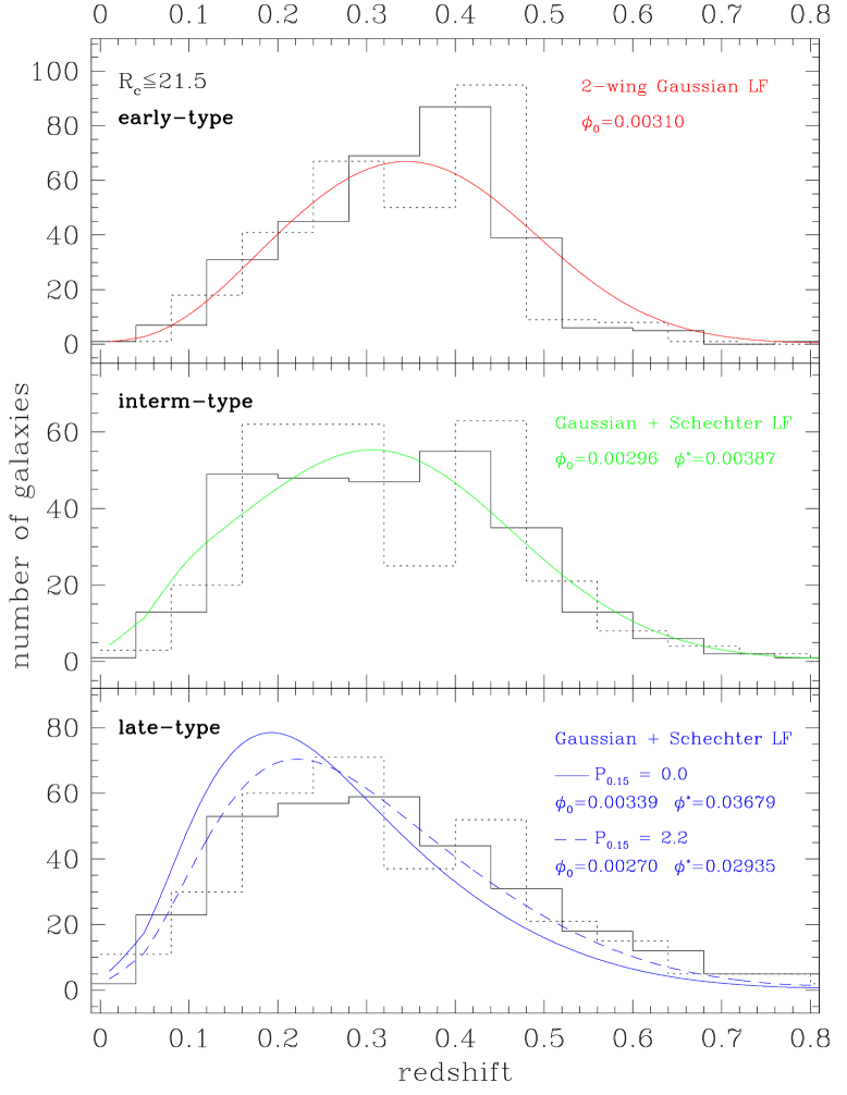
Figure 13: The observed redshift distribution for the early-type (top graph), intermediate-type (middle graph), and late-type galaxies (bottom graph) in the ESS $R_{\mathrm{c}}\leq 21.5$ sample. In order to allow for the noise in the observed histograms, these are plotted for 2 binnings of $\Delta z=0.08$, offset by $0.04$ in redshift (first bin starting at $z=0$, $z=0.04$ for the dotted, resp. solid histogram). The expected distribution for a uniform galaxy distribution with the ESS incompleteness and the composite luminosity function listed in Table 1 is over-plotted as a solid line for the 3 spectral classes. For the late-type galaxies, we also plot as a dashed line the expected distribution with an evolution factor $P_{0.15}=2.2$, as derived from the $R_{\mathrm{c}}$ number counts (see Sect. 6). All expected curves are normalized so that they match the observed number of galaxies in the interval $0.01\leq z\leq 0.81$; the resulting amplitudes $\phi_{0}$ and $\phi^{*}$ for the Gaussian and Schechter components are indicated inside each panel.

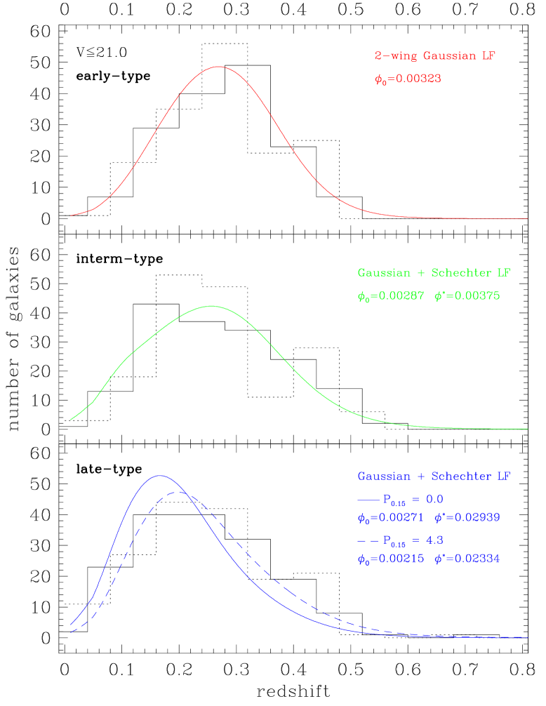
Figure 14: Same as Fig. 13 for the ESS $V\leq 21.0$ sample, with $P_{0.15}=4.3$ as derived from the $V$ number counts (see Sect. 6).

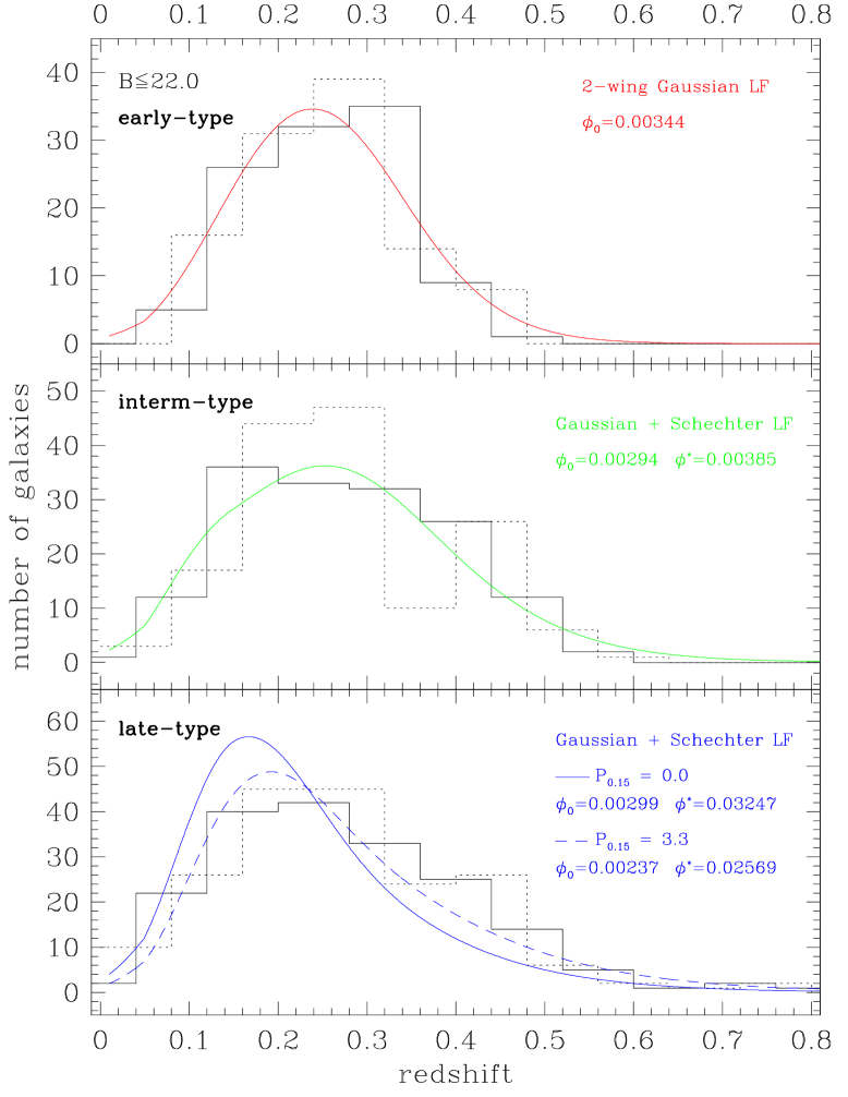
Figure 15: Same as Fig. 13 for the ESS $B\leq 22.0$ sample, with $P_{0.15}=3.3$ as derived from the $B$ number counts (see Sect. 6).

As in Sect. 5.1, the expected curves in Figs. 13, 14, and 15 are based on the integral of the selection function over the bin-size $\Delta z=0.08$, and we use the K-corrections calculated for the average spectral-type $<T_{\mathrm{S}}>$ among each spectral class (see Eq. 1). For the 3 galaxy types and in the 3 filters, the amplitudes $\phi_{0}$ and $\phi^{*}$ defining each non-evolving expected curve are defined by normalizing the integral of the expected distribution to the observed number of galaxies in the interval $0.01\leq z\leq 0.81$ (the ratio $\phi_{0}/0.4\ln 10\;\phi^{*}$ takes the values listed in Table 1). The resulting values of $\phi_{0}$ and $\phi^{*}$ are indicated inside each graph of Figs. 13 to 15, and are also listed in Table 3 in column labeled ($\Omega_{m}$,$\Omega_{\Lambda}$)=(0.3,0.7). These values of $\phi_{0}$ differ from the estimates $\Phi_{3}(0.51)$ listed in Table 2, because the latter result from an integral over the narrower redshift interval $0.1\leq z\leq 0.51$ (see Sect. 5.3).

For the early-type and intermediate-type galaxies, the expected distributions in Figs. 13, 14 and 15 provide a good match to the observed histograms. For the late-type galaxies, the expected no-evolution redshift curves (with $P_{0.15}=0.0$) show a systematic shift towards low redshifts when compared to the observed distributions. Moreover, the expected curves lie systematically near the lower values of the observed histograms for $z\ga 0.3$. These effects are present in the 3 filters.

For the late-type galaxies, we also plot in Figs. 13, 14 and 15 the expected redshift distributions with the values of the evolution factor $P_{0.15}$ listed in Table 4 for ($\Omega_{m}$,$\Omega_{\Lambda}$)=(0.3,0.7). The values of $\phi_{0}(0.15)$ and $\phi^{*}(0.15)$ which normalize the integral of each evolving distribution to the corresponding observed number of galaxies in the interval $0.01\leq z\leq 0.81$ are indicated in Figs. 13 to 15. Note that these values differ from those listed in Table 4, as the latter are derived by normalization to the total number-counts. The difference is however small, $\la 10$%, thus bringing a posteriori evidence of consistency between the redshift and magnitude distributions. Note also that in the evolving curves, we have extrapolated to $0\leq z\leq 0.15$ the linear evolution of $\Phi$ for the late-type galaxies parameterized in Eq. 20, although it was measured from the restricted redshift interval $0.15\leq z\leq 0.5$. Our motivations for this choice are:

• if we assume that $\Phi$ remains constant and at the value of the linear fit at $z=0.15$ for redshifts $\leq 0.15$, the expected redshift distributions show an marked excess of galaxies at these redshifts, which does not match the observed distribution (this effect is observed in all filters).

• the location of the ESS was visually selected by examining copies of the ESO/SERC R and J atlas sky survey with the criteria to avoid nearby galaxies and nearby groups and clusters of galaxies. This implies that the ESS survey has a systematically low density of galaxies at $z\la 0.1$.

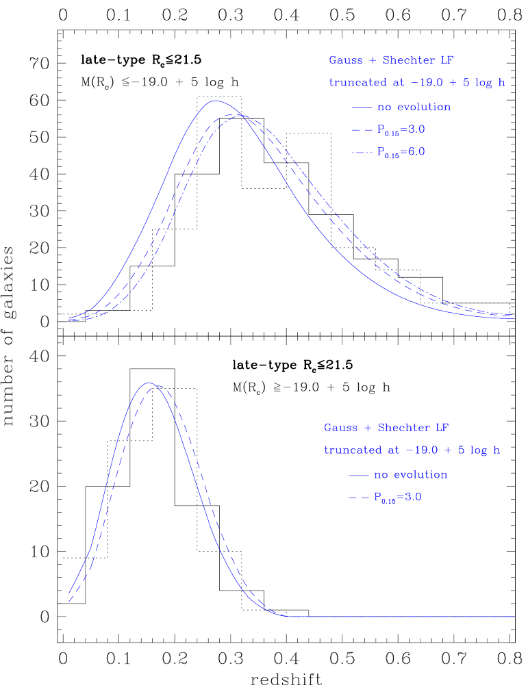
Figure 16: The observed redshift distribution for the bright and faint galaxies in the ESO-Sculptor late-type class ($M(R_{\mathrm{c}})\leq-19.0+5\log h$ in top panel, $M(R_{\mathrm{c}})\geq-19.0+5\log h$ in bottom panel). In order to allow for the noise in the observed histograms, they are plotted for 2 binnings of $\Delta z=0.08$, offset by $0.04$ in redshift (first bin starting at $z=0$, $z=0.04$ for the dotted, resp. solid histogram). The expected distribution for a uniform galaxy distribution with the ESS incompleteness and the composite late-type LF listed in Table 1 and truncated at $M(R_{\mathrm{c}})=-19.0+5\log h$ is plotted as a solid line in both panels. The expected distribution with an evolution factor $P_{0.15}=3.0$ is plotted as a dashed line in both panels; the expected curve with $P_{0.15}=6.0$ is also shown as a dash-dotted line in the top panel. The expected curves are normalized so that they match the observed number of galaxies in the interval $0.01\leq z\leq 0.81$.

In contrast to the no-evolution curves, the evolving late-type distributions provide a good match to the observed histograms in Figs. 13, 14 and 15: the low redshift peak is shifted to higher redshift ($z\ga 0.2$), and the high redshift tail has a higher amplitude which better matches the observed data. The best agreement of the observed and evolving expected curve is obtained in the $R_{\mathrm{c}}$ band (Fig. 13). In the $V$ and $B$ bands (Figs. 14 and 15), the expected curves with $P_{0.15}=4.3$ and $P_{0.15}=3.3$ resp. may be still be too low at $z\ga 0.3$. Using $P_{0.15}=7.0$ and $P_{0.15}=8.0$ in the $V$ and $B$ bands (as obtained from the direct fits of $\Phi_{1}$ in Sect. 5.3) yields a better match of the observed redshift distributions at $z\ga 0.3$, but systematically underestimate the distributions at $z\la 0.15$. This may be an indication that extrapolation of the linear model of Eq. 20 to $z\leq 0.15$ is not satisfying for large values of $P_{0.15}$. The varying incompleteness with galaxy type which affects the $V$ and $B$ samples is also likely to complicate the adjustment of the redshift distributions.

Note that the incompleteness of the full sample is used to correct for the incompleteness in apparent magnitude of each spectral-type sample in Figs. 13, 14 and 15. Ideally, one should use the incompleteness calculated for each spectral class. However, galaxies with no redshift measurement have no spectral-type determination. We have examined the dependence of the incompleteness as a function of galaxy-type using the colors of the galaxies without redshift, as these are correlated with galaxy type. For the $R_{\mathrm{c}}\leq 20.5$ sample, the incompleteness is uniform with galaxy colors, justifying the use of the average incompleteness for the full sample. For the $V\leq 21.0$ and $B\leq 22.0$ samples, the incompleteness is significantly stronger for the bluer galaxies; we cannot however evaluate the incompleteness per spectral-type from the colors as the relation between color and spectral-type suffers a large dispersion. The relative larger incompleteness in blue galaxies at faint magnitudes of the $V$ and $B$ spectroscopic samples converts into a relative larger incompleteness in faint late-type galaxies compared to early-type galaxies. This might explain why the expected curves for the late-type galaxies in Figs. 14 and 15 appear to systematically under-estimate the observed distribution.

As already mentioned in Sect. 3, the ESS late-type class contains predominantly Sc+Sd and dI galaxies. An interesting issue is how the giant (Sc+Sd) and dwarf (dI) galaxies contribute to this evolution. In the composite fit to the late-type LF at $R_{\mathrm{c}}\leq 21.5$ shown in the lower left panel of Fig. 1, the giant and dwarf components cross-over near $M(R_{\mathrm{c}})\simeq-18.5+5\log h$ for $(\Omega_{m},\Omega_{\Lambda}$)=(1.0,0.0); for $(\Omega_{m},\Omega_{\Lambda}$)=(0.3,0.7), this magnitude converts approximately to $M(R_{\mathrm{c}})\simeq-18.8+5\log h$ (see Sect. 4). We therefore calculate the observed and expected redshift distributions for the 2 following sub-samples: the bright sample, with $M(R_{\mathrm{c}})\leq-19.0+5\log h$, containing 227 galaxies, which are predominantly Sc+Sd galaxies; the faint sample, with $M(R_{\mathrm{c}})\geq-19.0+5\log h$, containing 82 galaxies, which are predominantly dI galaxies. Lower panel of Fig. 16 shows that an evolution factor with $P_{0.15}=3.0$ has a small impact on the distribution of galaxies with $M(R_{\mathrm{c}})\geq-19.0+5\log h$, and both expected curves are compatible with the observed distribution. In contrast, the expected no evolution curve provides a poor match to the observed distribution of galaxies with $M(R_{\mathrm{c}})\leq-19.0+5\log h$, whereas the expected curve with $P_{0.15}=3.0$ provides a better agreement. The expected distribution for a higher evolution rate, $P_{0.15}=6.0$, is also shown in Fig. 16 for the bright galaxies: it provides an even better adjustment (note that if the dI galaxies where not evolving, a higher evolution rate than measured for the Sc+Sd+dI altogether would be expected for the Sc+Sd galaxies alone). This suggests that the Sc+Sd galaxies are likely to contribute significantly to the detected late-type evolution. We however cannot exclude evolution of the dI galaxies.

8 Comparison of the ESS evolution with other surveys

Most other redshift surveys to $z\sim 0.5-1.0$ detect evolution in the luminosity function. The evolution affects either the amplitude $\Phi$ of the LF (number-density evolution), or its shape via the characteristic magnitude (luminosity evolution) and/or its faint-end behavior. Evolution in the luminosity density is also often used for measuring the evolution rate, as it has the advantage to account for the 3 types of evolution. Note that for a non-evolving shape of the luminosity function $\varphi(M)\mathrm{d}M$ , any evolution in the amplitude $\Phi$ (see Eq. 7) yields an identical evolution rate of the luminosity density.

In the following, we only consider the evidence for separate evolution of the E/S0 and Spiral galaxies, as evolution in the full galaxy population does not allow one to isolate the evolving population. For instance, the total luminosity density $\rho_{L}$ in the CFRS shows an increase with redshift which Lilly et al. (1996) model as $\rho_{L}(z)\propto(1+z)^{2.7\pm 0.5}$ at 4400 Å for an ($\Omega_{m}$,$\Omega_{\Lambda}$)=(1.0,0.0) cosmology. This is close to the value $\gamma=2.6$ obtained from the ESS $B$ band number-counts in Table 4, suggesting that the evolution rate for the Spiral galaxies in the CFRS may be higher than in the ESS. A direct measure of the evolution rate of the blue galaxies in the CFRS (bluer than a non-evolving Sbc galaxy) would however be required for a quantitative comparison with the ESS.

Because there is weak evidence for evolution in the faint-end slope of the LF in the existing surveys (Heyl et al., 1997), we restrict the following discussion to the evidence for (i) number-density evolution, and (ii) luminosity evolution.

8.1 Number-density evolution

Ellis et al. (1996) detect a marked density evolution in the Autofib star-forming galaxies by a factor 2 between $z\sim 0.15$ and $z\sim 0.4$, which would correspond to an overall fading of the population by $0.5$^mag  in the $b_{J}$ band. This is comparable to the ESS evolution rate derived above: for $P_{0.15}=3.0$, the density increases by a factor $1.75$ between $z\sim 0.15$ and $z\sim 0.4$. Further analysis of the Autofib survey based on galaxy spectral types (Heyl et al., 1997) leads to detection of a strong density evolution in the late-type spiral galaxies (Sbc and Scd) which they model as $\phi^{*}(z)\propto(1+z)^{2.9}$ for the Sbc galaxies and as $\phi^{*}(z)\propto(1+z)^{3.5}$ for the Scd galaxies in a cosmology with ($\Omega_{m}$,$\Omega_{\Lambda}$)=(1.0,0.0). These values are in acceptable agreement with the $\gamma=2.6$ value derived from the ESS in the $B$ band.

In the CNOC2, the dominant evolution detected by Lin et al. (1999) in the redshift range $0.1\la z\la 0.55$ is a strong density evolution of the late-type galaxies, defined as galaxies with $UBVR_{\mathrm{c}}I_{\mathrm{c}}$ colors similar to those computed from the Scd and Im templates of Coleman et al. (1980); the authors model the evolution as $\phi^{*}(z)\propto e^{Pz}$, with $P=2.8\pm 1.0$ and $P=2.3\pm 1.0$ in the $B_{AB}$ band for $\Omega_{m}=1.0$, $\Omega_{m}=0.2$ resp.; and $P=2.9\pm 1.0$, $P=2.6\pm 1.0$ in the $R_{\mathrm{c}}$ band for $\Omega_{m}=1.0$, $\Omega_{m}=0.2$ respectively. At $z\la 0.1$, $e^{Pz}$ and $(1+z)^{\gamma}$ can be expanded into $1+Pz$ and $1+\gamma z$ resp., which would yield a reasonable agreement at low redshift between the CNOC2 and the ESS in both the $B$ and $R_{\mathrm{c}}$ bands. However, at $z\sim 1$, $e^{2.5z}$ is a factor of 2 larger than $(1+z)^{2.5}$, implying a stronger evolution rate in the CNOC2 than in the ESS.

Obtained with a similar observational technique as the CNOC2, the field sample of the CNOC1 (Lin et al., 1997) shows an increase of the luminosity density of galaxies by a factor 3 between $z\sim 0.25$ and $z\sim 0.55$ for galaxies with rest-frame colors bluer than a non-evolving Sbc galaxy. In the NORRIS survey of the Corona Borealis Supercluster, Small et al. (1997b) detect a similar evolution rate: the amplitude $\phi^{*}$ of the Schechter LF for galaxies with strong [OII] emission line increases by nearly a factor 3 from $z\la 0.2$ to $0.2\leq z\leq 0.5$. These various values of the number-density evolution rate are stronger than the increase by a factor $1.8$ in the ESS density of late-type galaxies which we derive for $P_{0.15}=3.0$ between $z\sim 0.2$ et $z\sim 0.5$.

In the CADIS survey, in which redshifts are derived from a combination of wide and medium-band filters, Fried et al. (2001) detect an increase of the Johnson $B$ luminosity density of Sa-Sc galaxies with redshift, which is partly due to an increase in the amplitude $\phi^{*}$ of the fitted Schechter luminosity function, and can be modeled as $\rho(z)\propto(1+6.9z)$ for ($\Omega_{m}$,$\Omega_{\Lambda}$)=(1.0,0.0), and as $\rho(z)\propto(1+0.78z)$ for ($\Omega_{m}$,$\Omega_{\Lambda}$)=(0.3,0.7). The evolving term in the luminosity density can be converted into $\rho(z)\propto[1+3.4(z-0.15)]$, resp. $\rho(z)\propto[1+0.70(z-0.15)]$. Whereas the CADIS evolution rate is similar to that in the ESS for ($\Omega_{m}$,$\Omega_{\Lambda}$)=(1.0,0.0), it is much smaller than in the ESS for ($\Omega_{m}$,$\Omega_{\Lambda}$)=(0.3,0.7) (see Table 4); note however that this comparison may be complicated by the fact that the considered evolving CADIS population contains early-type Spiral galaxies, to the contrary of the ESS late-type spectral class.

In contrast, the recent COMBO-17 survey (Wolf et al., 2003) which is also based on a combination of wide and medium-band filters, shows no significant evolution in the number-density and luminosity density of either Sa-Sc and Sbc-Starburst galaxies from $z\sim 0.3$ to $z\sim 1.1$ in the Johnson $B$ and SDSS $r$ bands (Fukugita et al., 1996). Moreover, whereas the various mentioned surveys (CFRS, Autofib, NORRIS, CNOC2, CNOC1, CADIS) show no or a weak change in the luminosity density of early-type (E-S0) or red galaxies over the considered redshift range, the COMBO-17 survey detects a marked increase with redshift by a factor of 4 in the contribution from the E-Sa galaxies to the $r$ and $B$ luminosity densities for ($\Omega_{m}$,$\Omega_{\Lambda}$)=(0.3,0.7) (Wolf et al., 2003). The different results between the COMBO-17 and the other redshift surveys may be due to the complex selection effects inherent to surveys based on multi-medium-band photometry such as the COMBO-17, and which are most critical for emission-line galaxies. These effects however do not seem to affect the CADIS survey.

At last, the evolution detected in the far infrared from IRAS galaxies (Saunders et al., 1990; Bertin et al., 1997; Takeuchi et al., 2003) can be characterized as $\phi^{*}(z)\propto(1+z)^{\gamma}$ with $\gamma\simeq 3-3.4$ for pure density evolution (both cosmologies considered in this article are used, depending on the authors). The evolution of the IRAS galaxies is consistent with the ESS late-type evolution, in agreement with the fact that IRAS galaxies may represent a sub-population of the optical spiral galaxies.

8.2 Luminosity evolution

The apparent density evolution detected in the ESS could also be produced by a luminosity evolution of the late-type spiral galaxies: if these galaxies were brighter at higher redshift, they would enter the survey in larger numbers at a given apparent magnitude. Using the values of the power-law index $\gamma$ listed in Table 4 and the slopes of the ESS magnitude number-counts (Arnouts et al., 1997), we can estimate a corresponding magnitude brightening. For cosmological parameters ($\Omega_{m}$,$\Omega_{\Lambda}$)=(1.0,0.0), we measure from Table 4 an increase in the number-density of galaxies by a factor $2.8$ between $z\simeq 0$ and $z\simeq 0.5$, and by a factor $5.7$ between $z\simeq 0.5$ and $z\simeq 1$ in the $R_{\mathrm{c}}$ band; in the $B$ bands, the density increases by a factor $2.9$ at $z\simeq 0.5$, and $6.1$ at $z\simeq 1$. For ($\Omega_{m}$,$\Omega_{\Lambda}$)=(0.3,0.7), the density increases by $2.1$ and $3.5$ at $z\simeq 0.5$ and $z\simeq 1$ resp. in $R_{\mathrm{c}}$, and by $2.4$ and $4.6$ at $z\simeq 0.5$ and $z\simeq 1$ resp. in $B$. Using the slopes $\beta=0.38$ in the $R_{\mathrm{c}}$ band and $\beta=0.46$ in the $B$ band ($n(m)\propto 10^{\beta m}$) for the ESS magnitude number-counts (Arnouts et al., 1997), these values of the density increase are equivalent to $\sim 1.2$^mag and $\sim 2.0$^mag brightening of the late-type ESS galaxies at $z\simeq 0.5$ and $z\simeq 1$ resp. in $R_{\mathrm{c}}$, and a $\sim 1.1$^mag and a $\sim 1.7$^mag brightening resp. in $B$ for ($\Omega_{m}$,$\Omega_{\Lambda}$)=(1.0,0.0); and to $\sim 0.8$^mag  and $\sim 1.4$^mag brightening resp. in both the $R_{\mathrm{c}}$ and $B$ bands for ($\Omega_{m}$,$\Omega_{\Lambda}$)=(0.3,0.7) (the steeper evolution rate in the $B$ band is compensated by a steeper slope of the number-counts also in the $B$ band).

These brightening estimates for the ESS late-type galaxies with ($\Omega_{m}$,$\Omega_{\Lambda}$)=(0.3,0.7) are comparable to those caused by the passive evolution of an Sc galaxy (due to the evolution of the stellar population). From the model predictions of Poggianti (1997, using ($\Omega_{m}$,$\Omega_{\Lambda}$)=(0.45,0.0) and $H_{0}=50$ km s^-1 Mpc^-1, which imply an age of the Universe of 15 Gyr), an Sc galaxy brightens by $\sim 0.6$^mag and $\sim 1.2$^mag in its rest-frame $R$ band at $z\sim 0.5$ and $z\sim 1.0$ resp., and by $\sim 0.9$^mag, $\sim 1.5$^mag resp. in its rest-frame $B$ band. A comparable or stronger brightening is expected for the Elliptical galaxies at these redshifts: $\sim 0.6$^mag  and $\sim 1.4$^mag  in $R$, $\sim 0.7$^mag  and $\sim 3.0$^mag  in $B$ (Poggianti, 1997). However, there are indications of a marked decrease in the number density of E galaxies with redshift (Fried et al., 2001; Wolf et al., 2003), which compensates for their luminosity evolution, which explains why no evolution in this population is detected by the ESS.

Lilly et al. (1995) detect a 1^mag brightening of the CFRS blue galaxies (defined as galaxies with rest-frame colors bluer than a non-evolving Sbc template from Coleman et al. 1980) between the intervals $0.2\la z\la 0.5$ and $0.5\la z\la 0.75$ in an ($\Omega_{m}$,$\Omega_{\Lambda}$)=(1.0,0.0) cosmology; they however cannot discriminate whether this brightening is due to luminosity or density evolution. With $\gamma=2.6$ (see Table 4), the ESS $B$ density of late-type galaxies increases by a factor $1.6$ between $z\simeq 0.25$ and $z\simeq 0.625$ (the median value of the 2 quoted CFRS intervals), which corresponds to a brightening of $\sim 0.44$^mag, nearly a factor 2 smaller than in the CFRS. Cohen (2002) also detect for the emission-line dominated galaxies at $z\sim 1$, when compared to the measurement of Lin et al. (1996) at $z\sim 0$, a mild brightening by $\sim 0.75$^mag in the $R$ band for an ($\Omega_{m}$,$\Omega_{\Lambda}$)=(0.3,0.0) cosmology, which is a factor 2 smaller than in the ESS estimated brightening in the $R_{\mathrm{c}}$ band for ($\Omega_{m}$,$\Omega_{\Lambda}$)=(0.3,0.7).

9 Conclusions, further discussion and prospects

Using the Gaussian+Schechter composite LFs measured for the ESO-Sculptor Survey, we obtain evidence for evolution in the late spectral-type population containing late-type Spiral (Sc+Sd) and dwarf Irregular galaxies. This evolution is detected as an increase of the galaxy density $n(z)$ which can be modeled as $n(z)\propto 1+P_{0.15}(z-0.15)$ with $P_{0.15}\sim 3\pm 1$ or as $n(z)\propto(1+z)^{\gamma}$ with $\gamma\sim 2\pm 1$ using the currently favored cosmological parameters ($\Omega_{m}$,$\Omega_{\Lambda}$)=(0.3,0.7); for ($\Omega_{m}$,$\Omega_{\Lambda}$)=(1.0,0.0), $P_{0.15}\sim 4\pm 1$ and $\gamma\sim 2.5\pm 1$. Both models yield a good match of the ESS $BVR_{\mathrm{c}}$ redshift distributions to $21-22$^mag and the number-counts to $23-23.5$^mag, which probe the galaxy distribution to redshifts $z\sim 0.5$ and $z\sim 1.0$ respectively. Using both the redshift distributions and the number-counts allows us to lift part of the degeneracies affecting faint galaxy number counts: the redshift distributions allow to isolate the evolving populations, whereas the faint number counts provide better constraints on the evolution rate. These results are based on the hypothesis that the shape of the LF for the ESS late-type class does not evolve with redshift out to $z\sim 1$.

Examination of the other existing redshift surveys to $z\sim 0.5-1.0$ indicates that a wide range of number-density evolution rates have been obtained. The evolution rate of the Sc+Sd+dI galaxies detected in the ESS is among the range of measured values, with some surveys having weaker of higher evolution rates. The most similar survey to the ESS, the CNOC2, yields a twice larger increase in the number density of late-type Spiral and Irregular galaxies at $z\sim 1$.

A priori, density evolution indicates that mergers could play a significant role in the evolution of late-type Spiral and Irregular galaxies. Le Fèvre et al. (2000) detect a $\sim 20$% increase in the fraction of galaxy mergers from $z\sim 0$ to $z\sim 1$, which can be modeled as $\propto(1+z)^{3.2}$; interestingly, examination of their Fig.1 indicates that a significant fraction of the merger galaxies have a Spiral or Irregular structure.

The ESS density increase for the Sc+Sd+dI galaxies could also be caused by a $\sim 1$^mag brightening of these galaxy populations at $z\sim 0.5$ and a $\sim 1.5-2.0$^mag brightening at $z\sim 1$ (depending on the filter and cosmological parameters). This luminosity evolution is compatible with the expected passive brightening of Sc galaxies at increasing redshifts (Poggianti, 1997). Driver (2001) also shows that the Hubble Deep Field (Williams et al., 1996) bi-variate brightness distributions for Elliptical, Spiral, and Irregular galaxies are all consistent with passive luminosity evolution in the 3 redshift bins $0.3-0.6$, $0.6-0.8$, $0.8-1.0$. The ESS brightening at $z\sim 1$ agrees with the value measured from the CFRS blue galaxies (Lilly et al., 1995), but is twice smaller than that measured by Cohen (2002) for emission-line dominated galaxies.

In all analyses of the redshift and magnitude distributions, the major difficulty is to distinguish between luminosity and density evolution, as these produce the same net effect on the redshift and magnitude distributions. Interpretation of density and luminosity evolution of a galaxy population is also complicated by possible variations in the star formation rate with cosmic time: Lilly et al. (1998) evaluate an increase in the star formation rate of galaxies with large disks by a factor of $\sim 3$ at $z\sim 0.7$, which shows as an increase of the luminosity density at bluer wavelengths. Using PEGASE (Fioc & Rocca-Volmerange, 1997), Rocca-Volmerange & Fioc (1999) also show that the Sa-Sbc galaxies have a star formation rate which varies more rapidly in the interval $0\la z\la 1$ than for the E/S0 or Sc-Im galaxies.

The ESS suggests that the Sc+Sd galaxies are an evolving population, but evolution in the dI galaxies cannot be excluded. Whether the Spiral galaxies, or the Irregular galaxies, or both populations contribute significantly to the excess number-counts is still unclear from the various existing analyses: using photometric redshifts, Liu et al. (1998) detected a significant amplitude increase and brightening of the $U$ LF of Sbc and bluer galaxies in the redshift interval $0\la z\la 0.5$, together with an excess population of starburst galaxies at $z\ga 0.3$ which are absent at $z\la 0.3$; galaxy number counts in the near infrared (Martini, 2001; Totani et al., 2001), which are less sensitive to current star formation, also allow some moderate number evolution of the Spiral galaxies and/or Irregular galaxies (with $\gamma\sim 1$, see above). Evolutionary effects are also detected at higher redshifts: Driver et al. (1998) show that at $1\la z\la 3$, the redshift distributions of Sabc galaxies to $I>25$ and of Sd/Irr galaxies to $I>24$ require some number and luminosity evolution (but see Driver, 2001). This could be consistent with the recent deep optical and infrared observations which favor mild luminosity evolution of the overall galaxy population (Pozzetti et al., 2003; Kashikawa et al., 2003). Nevertheless, none of these surveys allow one to isolate one evolving population among the Spiral and Irregular/Peculiar galaxies.

In contrast, some surveys favor Irregular/Peculiar galaxies as a major contributor to the excess count: an excess population of Irregular/Peculiar galaxies was directly identified as the cause for a strong deviation from no-evolution in the $I$ and $K$ number-counts per morphological type (Glazebrook et al., 1995; Huang et al., 1998); a population of gently-evolving starbursting dwarves was also invoked to explain these excess objects (Campos, 1997). Using morphology of galaxies obtained from Hubble Space Telescope images, Im et al. (1999) provide further evidence for a marked increase in the relative abundance of Irregular and Peculiar galaxies which they interpret as starbursting sub-$L^{*}$ E/S0 and Spiral galaxies. Totani & Yoshii (1998) also detect such an excess population at $z\ga 0.5$. Using again Hubble Space Telescope imaging for galaxy morphology, Brinchmann et al. (1998) estimate a $\sim 30$% increase in the proportion of galaxies with an irregular morphology at $0.7\la z\la 0.9$ (see also Abraham et al., 1996; Volonteri et al., 2000).

Other surveys identify Spiral galaxies as the evolving population: morphological number counts based on Hubble Space Telescope images indicate that the Spiral counts rise more steeply than the no-evolution model (Abraham et al., 1996). By complementing space-based images with ground-based spectroscopic redshifts, Brinchmann et al. (1998) detect a $\sim 1$^mag brightening of the Spiral galaxies by $z\sim 1$. Schade et al. (1996) also measure a $\sim 1.6$^mag brightening of the central surface brightness of galaxy disks at $0.5\la z\la 1.1$.

We emphasize that measuring a reliable evolution rate requires a realistic parameterization of the intrinsic LFs of each galaxy population. We show here that the ESS Gaussian+Schechter composite LFs provide more robust constraints on the evolution rate than pure Schechter LFs, as a small change in the faint-end slope has a large incidence onto the number-counts. In contrast, variations in the faint-end slope of the dE and dI galaxies, the only populations for which the Schechter faint-end is poorly determined have a smaller impact on the adjustment on the number counts. Totani et al. (2001) also show that separating the E and dE galaxies into a Gaussian+Schechter LF does yield a better agreement of the $K$ number-counts at $K\ga 22.5$ than a pure Schechter function for the joint class of E+dE.

By using better measures of the intrinsic LFs for the various galaxy types, one should be able to obtain improved measurements of the galaxy evolution rates, and eventually to use the faint number counts to probe the cosmological parameters. Koo et al. (1993) and Gronwall & Koo (1995) had already suggested that passive luminosity evolution is sufficient to match the $B$ number counts, thus implying that the number counts could be used to probe the curvature of space. Pozzetti et al. (1996) and Metcalfe et al. (2001) then showed that passive luminosity evolution with a low value of $\Omega_{m}$ provide good fits to UV-optical-near-infrared galaxy counts. The recent adjustments of very deep optical and near-infrared galaxy counts (Totani & Yoshii, 2000; Nagashima et al., 2001; Totani et al., 2001; Nagashima et al., 2002) which probe the galaxy distribution to $z\sim 3$ further confirm that the Einstein-de Sitter cosmology with ($\Omega_{m}$,$\Omega_{\Lambda}$)=(1.0,0.0) is excluded at a high confidence level (see also Totani et al., 1997; He et al., 2000); whereas by using the currently favored values of $\Omega_{m}=0.3$ and $\Omega_{\Lambda}=0.7$, these fits constrain the evolution rate of galaxies in the hierarchical clustering picture, with only some mild number evolution of Sbc/Sdm galaxies allowed (Totani et al., 2001).

Under-going deep redshift surveys to $z\ga 1$ raise new prospects along this line. The present ESS analysis shows the usefulness of using both the magnitude and redshift distributions for studying galaxy evolution. By obtaining the redshift distributions per galaxy type to $z\ga 1$ over large volumes which average out the large-scale structure, spectroscopic redshift survey such as the VIRMOS (Le Fevre & Vettolani, 2003) and DEEP2 (Davis et al., 2003) projects should provide improved clues on the evolving galaxy populations at $z\sim 1$ and better constrain the nature of this evolution. If these surveys confirm that all galaxy types only experience mild luminosity/density evolution, complementing the deep infrared galaxy counts with morphological information might allow one to lift the degeneracy in the faint infrared number-counts and to confirm whether a low matter-density universe is favored. This will however require a detailed knowledge (i) of the luminosity-size relation for distant galaxies of various morphological type (used to model the selection effects caused by the cosmological dimming in surface brightness, see Totani & Yoshii 2000), and (ii) of the interstellar and intergalactic extinction.