SLAC–PUB–10276
26 March 2004

Abstract

We define a universe as the contents of a spacetime box with comoving walls, large enough to contain essentially all phenomena that can be conceivably measured. The initial time is taken as the epoch when the lowest CMB modes undergo horizon crossing, and the final time taken when the wavelengths of CMB photons are comparable with the Hubble scale, i.e. with the nominal size of the universe. This allows the definition of a local ensemble of similarly constructed universes, using only modest extrapolations of the observed behavior of the cosmos. We then assume that further out in spacetime, similar universes can be constructed but containing different standard model parameters. Within this multiverse ensemble, it is assumed that the standard model parameters are strongly correlated with size, i.e. with the value of the inverse Hubble parameter at the final time, in a manner as previously suggested. This allows an estimate of the range of sizes which allow life as we know it, and invites a speculation regarding the most natural distribution of sizes. If small sizes are favored, this in turn allows some understanding of the hierarchy problems of particle physics. Subsequent sections of the paper explore other possible implications. In all cases, the approach is as bottoms up and as phenomenological as possible, and suggests that theories of the multiverse so constructed may in fact lay some claim of being scientific.

1 Introduction

The idea that the universe we see around us is a member of an ensemble of universes (the multiverse), the remainder of which are beyond our view, is an old one, But it is one under active investigation nowadays. Much of the contemporary motivation comes from rather grandiose theoretical conceptualizations. These include, but are not limited to, string theory ideology, eternal inflation, and even Everett’s many-worlds interpretation of quantum mechanics [1].

But another motivation comes from the great progress being made in the experimental investigation of the structure and early history of our own universe, as well as the successful establishment of the standard model of particle physics. While the accumulation of these data is no doubt the best stimulant, it nevertheless has led to a mixing of direct information from the experiments with highly speculative material, remote from experimental test. Indeed, there is plenty of skepticism extant as to whether the consideration of universes which are causally disconnected from our own is science at all.

The purpose of this note is to make the study of ensembles of universes as data-driven as possible. This will entail, first, a specific definition of a universe as the contents of a comoving spacetime box, large enough to contain essentially everything we can expect to be able to measure (based on the present consensus picture of cosmology and particle physics), but still small compared to the extent of the total spacetime domain envisaged by the majority of cosmologists and other theorists. This allows a credible way of constructing a local ensemble of universes very similar to our own. One simply generalizes the construction of our universe to other spacetime domains causally disconnected from our own, yet near enough to allow reasonable extrapolation of properties of our universe to the remainder of the local ensemble.

We envisage this construction of our universe in analogy to the establishment of a homestead in Kansas by a pioneer family. They would see their spatial environment, as we do see our universe, as flatter than a pancake [2], all the way to their property line. And it would be not unreasonable—and in fact even correct—for them to envisage other similar homesteads beyond their horizon. Were the family to contain a theorist, he or she would in fact probably erroneously conclude that Kansas, and hence the number of such homesteads, in fact was infinite in extent [3]. However, far beyond Kansas will be found other pieces of fertile terrain, e.g. in the Central Valley of California, which also are flatter than a pancake and which bear other similarities to, as well as differences from, the Kansas homesteads.

The local, “Kansas” ensemble of universes we shall consider will be assumed to possess a spatially flat FRW metric, with similar initial cosmological boundary conditions. This ensemble is already phenomenologically of some use, because it can be considered as the ensemble implicitly used by inflationary cosmologists in making quantum averages of the inflationary perturbation spectra. But more interesting, and the focus of this note, are the analogues of the Central Valley homesteads. We take these to be similar to our universe in the sense of again being described by a spatially flat FRW metric, with perhaps some also being fertile, i.e. capable of supporting life as we know it. The features that we assume can vary from universe to universe will include the parameters of the standard model and of cosmology.

One can generalize much further than this, at the cost of increasing the level of speculation [4]. We will stop at this point, however. The reasons are, first, that obviously this level is already quite speculative, and second, that the data-driven (as well as theoretical!) motivations for considering ensembles of universes can already be expressed with specificity at this level of speculation. The main data-driven consideration is that the values of many standard model parameters seem to be fine-tuned in a way to allow our existence in the universe. The existence of an ensemble of universes with a variety of standard-model parameters allows an “anthropic” interpretation of this property of standard-model data [1, 5]. And the main theoretical consideration comes from string theory, where a variety of string vacuua, with different standard-model properties, may easily be envisaged to occur in various causally disconnected regions of spacetime [6].

These issues can all begin to be addressed in the context of the subensemble of universes that we construct, namely those that differ in a rather minimal way from our own. It is already of great interest to try to delineate the existence and properties of these “nearest-neighbor” universes. And the possibility of erroneous speculation, while still huge, is clearly going to be less than dealing (in the absence of data) with a more broadly generalized ensemble of universes possessing properties vastly different from our own.

Another analogy to the ensemble of universes is the perhaps familiar one of the planets in our own universe. These are already known to come in many varieties, but an especially interesting subset of planets consists of those containing life as we know it. This “nearest-neighbor” ensemble might consist of only Planet Earth, or it may contain a large number [7]. The question of which alternative is correct is not only irresistible to ask, but is also undeniably a scientific one. In order to address it in a systematic way, one needs to parametrize properties of planets in such a way that one can look at the distribution function of those parameters and find the size and location of the habitable island in parameter space. The output of such a program could be an estimate or bound on the number of planets which can in principle support life as we know it. This is in the case of planets a very daunting task, one that will need to be data-driven to make progress [8]. If universes as we have defined them have a similarly complex parametrization, it will be extremely difficult to make progress, simply due to lack of data. It is a serious criticism by those who remain skeptical of the utility of multiverse ideology that this problem presents an insuperable barrier to scientific consideration of this line of thinking.

The use of “anthropic” reasoning when dealing with ensembles of universes only exacerbates this problem. If the distribution function of standard model parameters, taken over the multiverse ensemble, is broad in each of the parameters, and if there is little correlation between the probability of finding the value of one parameter and that of another, then the program of finding naturalistic explanations for the values of standard model parameters essentially grinds to a halt. The replacement is a statement, unsupported by data, that they are determined by historical accident. To this author, such an option seems not much more scientific in nature than interpreting the values of the standard model parameters via “intelligent design”.

However, we cannot ourselves impose a decision on how things work at this level. If the above option is true, then it may be that the scientific method will never have the power to find out the answers to the Big Questions. But, it is not clear that the problem of characterizing the ensemble of universes is in fact as difficult as characterizing the ensemble of habitable planets. As long as there is an outside chance that the problem is simpler and more tractable, there is no reason not to pursue that possibility. This optimistic position will in fact be our working assumption. We shall assume that many of the standard model parameters are strongly correlated with each other, thereby simplifying the nature of the aforementioned distribution function. While anthropic reasoning will be utilized, the amount will be limited by the above simplistic assumption of the existence of correlations. And the test of whether the assumption makes sense will be whether it delivers insight into any of the unsolved problems facing particle physics and cosmology. We shall argue on the basis of the results that the answer to this is positive. In particular we shall obtain a partial understanding of the nature of the hierarchy problems of particle physics: why the ratios of many of the standard model parameters are such large numbers. We do not claim that the hierarchy problems are thereby solved, but rather that they are recast in a different form, one which in turn appears to be able to be attacked by scientific methods.

In the next section, we discuss in detail our definition of a universe, and in Section 3 provide a concise description of its major properties. In Section 4 we review the nature of our assumed correlations of standard model parameters , emphasizing their simplicity and cogency, as well as the consequence that the habitable range of sizes is limited to within a factor two of the size of our universe. In Section 5, we discuss the anthropic implications of this scenario, in particular that if the distribution in sizes is peaked at small sizes, there results some understanding of the hierarchy problems of particle physics.

The above material contains the main messages of this paper. The remaining sections are spinoff topics even more speculative. Section 6 explores a possible connection between Bekenstein-Hawking horizon entropy and the vacuum structure of QCD. Section 7 explores whether the inflationary phase of our universe might have its own set of standard model parameters, correlated with the very large value of the Hubble parameter (dark energy) during that epoch. Section 8 raises the question of whether the starting time we have used in our construction of the universe may contain physics, and represent the actual onset of the inflationary epoch. Section 9 is devoted to concluding comments.

2 The Standard Universe

We define our universe in rough terms as “what we and our descendants can observe in principle, plus a little more”. To be more specific, we need some mild assumptions, mild at least in comparison to others which will follow. They include:

1) The observable universe obeys on large scales the cosmological principle, and is described by the FRW metric.

2) The observable universe is spatially flat.

3) In the distant future, the universe will reinflate, i.e. be characterized by a nonvanishing cosmological constant. We also assume that quintessence is either absent or unimportant on the time scales which we consider.

4) The broad history of our universe is well-described by the “concordance model”: an inflationary epoch, followed by “reheating”, the radiation-dominated big bang, and subsequent events, as described in standard texts and references [9].

5) Our preferred inflationary scenarios lie in the category of “hybrid” models [10]. In particular we assume that the evolution during the inflationary epoch we consider is “quasi-deSitter”, with, to good accuracy, a nearly time-independent Hubble parameter.

With these assumptions, we may now map out the spacetime region of the observable portion of the universe. To do this we start with the form of the FRW metric

$$ds^{2}=dt^{2}-a^{2}(t)[d\theta^{2}_{x}+d\theta^{2}_{y}+d\theta^{2}_{z}]\ .$$ (1)

All the information is codified in the time dependence of the scale factor $a(t)$. Its dynamics is determined in a simple way by the Einstein equations, which we write down later. But before discussing that we introduce another useful set of coordinates, the “conformally flat coordinates”. The time $t$ is traded in for “conformal time” $\eta$, defined as

$$\eta=-\int^{\infty}_{t}\ \frac{dt}{a(t)}\qquad d\eta=\frac{dt}{a(t)}\ .$$ (2)

Therefore the line element in Eq. (1) becomes

$$ds^{2}=a^{2}(t)[d\eta^{2}-d\theta^{2}_{x}-d\theta^{2}_{y}-d\theta^{2}_{z}]\ .$$ (3)

The great usefulness of this choice is the clarity in seeing the causal connection between different spacetime events, since the trajectories of light rays in these coordinates are straight lines at 45 degrees to the vertical, just as in Minkowski spacetime. Therefore the portion of the FRW spacetime which we can see is a past light cone emanating from our worldline, which evidently is along the (conformal) time axis.

Important is the fact, implied in Eq. (2), that infinite FRW time maps into a finite, maximal conformal time. This occurs because of the existence of dark energy. The big-bang power-law growth of $a(t)$ morphs into an exponential growth once the dark energy becomes the dominant source term in the Einstein equations, thereby providing convergence for the integral in Eq. (2). At present, we already are able to see a large fraction of the spacetime that any distant descendants of us will be able to see. The past lightcone emanating from the $t=\infty$ (or $\eta=0$) point on our worldline, as shown in Fig. 1, provides a natural boundary between what is clearly a part of our own universe (as defined in the beginning of this section) and what is arguably beyond. This boundary surface is called by Hawking and Ellis [11] the “future event horizon”.

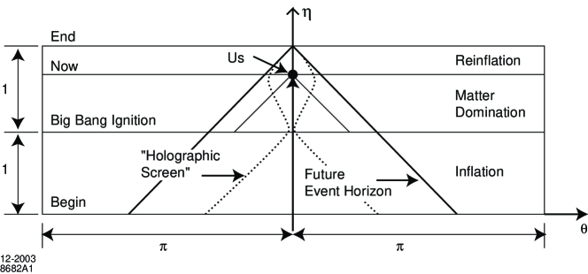
Figure 1: “Conformal” spacetime. The surface marked “holographic screen” is simply defined by $r=a(\eta)|\,\vec{\!\theta}\,|=H^{-1}(\eta)$.

While we might entertain defining the future event horizon as the boundary of our universe, we shall not do so. Instead, we shall define it as the interior of a comoving box. This is defined at any particular $t$ or $\eta$ as an ordinary box of physical size $L=2\pi a(t)$ on a side, with any point on that box moving along the $t$ or $\eta$ axis. This means that at sufficiently early times the box will lie inside the future event horizon. However our experimental access to extremely early times is both in practice and in principle very limited. So we shall also limit the spacetime of our universe to be in the future of some initial FRW time. This time is defined, roughly, as the time when, say, the dipole component of the cosmic microwave background undergoes “horizon crossing”, although the exact choice is negotiable. However, at this initial time, we shall require that the size of our comoving box be larger than the size of the future event horizon.

Likewise, we shall terminate the universe at a future time, of about one trillion years. This is a landmark time; the cosmic microwave background radiation is redshifted so much that the wavelength of the photons becomes comparable to the characteristic size of the universe. Thereafter, all the galaxies except those in our local cluster will have receded from view and the visible part of the universe will be filled with Hawking radiation of a wavelength typical of the size scale of the universe. The “classical” phase of the accelerated, dark-energy driven, deSitter expansion of the universe will terminate and be supplanted by the quantum deSitter expansion, about which there is much more theoretical uncertainty [12] and angst. So it seems like a good occasion for drawing the line between credible extrapolation and less credible speculations.

The net effect of these constructions is to define a spacetime box, within which lies essentially all the phenomenology that we can presently perceive and access, and beyond which exists a huge amount of theoretical and philosophical ideas, unsupported by data. The boundaries of the box are artificial, but it is unlikely that boundary effects exist that affect the phenomenology within. And the choice of a comoving box instead of some other boundary is strongly motivated by practical considerations. The graviton and inflaton modes which generate the cosmic microwave background texture are most simply described in terms of a mode expansion utilizing comoving-box boundary conditions, which we for simplicity take as periodic.

The contents of the spacetime box which we have constructed is by definition what we shall call a universe. Its parametrization, in particular the definition of the initial and final time surfaces, as well as choice of spatial size, will be discussed below in more detail. But before moving on, it should be emphasized that this definition of universe finesses many interesting questions, such as the origin of time, how and when the inflationary epoch begins, the ultimate fate of the universe, and the extent in space over which the FRW description remains valid. It is not that these questions are not important. But they are by definition “outside the box”, and therefore relatively remote from the issues that are accessible phenomenologically.

3 Describing the Universe

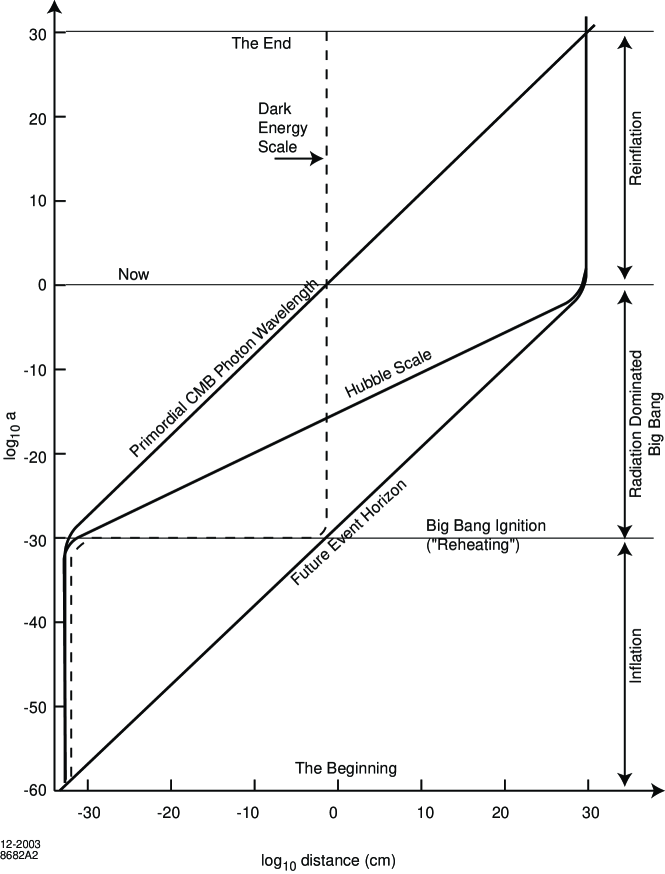
Figure 2: The “universe for dummies”.

The gross properties of our universe are encoded in the properties of the FRW scale factor $a(t)$, and in the dependence of other parameters of the universe on that quantity. We shall first look at these properties in a highly simplified limit, which we call ”the universe for dummies”. In this limit, we disregard the dark and hadronic matter content of the universe, and also disregard the difference between the scale of inflationary dark energy and the Planck scale. This involves setting various factors of up to $10^{5}$ to unity, but will involve keeping remaining factors of $10^{30}$ intact. The result is shown in Fig. 2, where on a log-log scale various quantities with dimension of distance are plotted against the scale factor, which in turn can be regarded as a time variable. These quantities include (1) the Hubble parameter

$$H=\frac{\dot{a}}{a}=\frac{d}{dt}\,(\ell n\,a)$$ (4)

(2) the magnitude of the characteristic dark energy distance scale $\mu^{-1}$ in the inflationary and present-day epochs. Here $\mu^{4}$ is the value of the dark energy density term in the standard-model Lagrangian density, related to the Hubble parameter of a dark-energy dominated expansion by

$$\mu^{4}=\frac{3}{8\pi}H^{2}M_{pl}^{2}\ ,$$ (5)

(3) the physical radius of the future event horizon $E(t)$, as discussed in the previous section, defined as

$$E(t)=a(t)|\eta|$$ (6)

and (4) the physical wavelength of the cosmic microwave background radiation.

We see from Fig. 2 that the basic architecture is characterized by three epochs of cosmic expansion, each characterized by an increase in the FRW scale factor $a(t)$ by a factor of about $10^{30}$. Likewise the ratio of cosmological scale to dark energy scale is again a factor $10^{30}$, as is the ratio of dark energy scale to the Planck scale. Evidently it is the cosmological constant which establishes this overall architecture.

We infer from this feature that the parameter most responsible for the gross features of our universe is in fact the cosmological constant. We consequently identify the intrinsic size of a universe with the value of its inverse Hubble parameter at late times, related to the cosmological constant by Eq. (5). We consider this definition of size to be an important characterization, perhaps the most important one, possessed by our universe and by other members of the ensemble of universes that we shall consider.

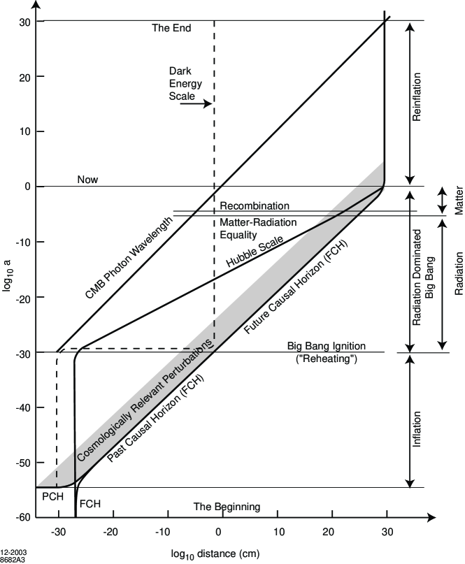
Figure 3: The real universe.

We also see from Fig. 2 that the initial time of our universe-in-a-box is naturally taken as when the value of the future event horizon is comparable to the value of the inverse of the Hubble parameter, and that the final time is naturally taken when the CMB wavelength is comparable to the inverse Hubble parameter.

A more realistic version of our universe is shown in Fig. 3. We have here included the modification of the evolution of the Hubble parameter due to the presence of dark matter. We also have parametrized the inflationary epoch more realistically, taking the inflationary dark energy scale to be of order the grand unification scale of about $10^{16}$ GeV, in rough concordance with the consensus value used by perhaps a majority of inflation theorists. This diminishes the Hubble parameter relative to the Planck scale by a very significant factor of about $10^{-5}-10^{-6}$. We also show in Fig. 3 the size of the inflationary perturbations relevant to phenomenology. One sees the “horizon-crossings”, namely the times at which the physical wavelengths of the perturbations are comparable to the inverse Hubble scale. It is clear from Fig. 3 that, as promised above, the initial time assumed in the construction of the spacetime box is comparable to the time when the lowest CMB multipoles “cross the horizon”. In fact it is more precisely defined by the requirement that the conformal time interval $\Delta\eta$ during inflation equals the $\Delta\eta$ from big-bang ignition to the final time we consider (essentially infinite FRW time $t$).

Our favorite choice for the size of the spacetime box is shown in Fig. 2. The spatial dimension is $2\pi$ larger than the duration of conformal time $\eta$ from reheating to the end, or from the beginning of inflation to the reheating time. This makes the values $k$ of the plane-wave mode expansion for the box in one to-one correspondence with the values of $\ell$ that our descendants at late times would use in analyzing the primordial CMB fluctuations. More importantly, this choice of spatial size should be large enough to make spurious boundary effects negligible phenomenologically, but without a great deal to spare [10].

A major advantage of the description of the evolution of the universe of Fig. 3 is that all the major epochs and distance or energy scales are readily visible in the plot; no features are squished into a tiny region. This is not the case in Fig. 1, where almost everything interesting is squished into the central line labelled “Big Bang Ignition” (reheating), or into the tip of the future-event-horizon light cone. There are only two epochs which really show clearly in Fig. 1. One is the present epoch, extending from a redshift of two or three in our past, to two or three efoldings of accelerated expansion in our future. The other epoch comprises the first few efoldings of inflation following the initial time we have specified for our universe. For completeness, we provide some mathematical details which further explain the two figures and their relationship in Appendix A.

4 Correlations of Standard Model Parameters

In the previous section, we argued that the most gross features of our universe, as determined by experimental cosmology, are characterized by the value of the asymptotic Hubble parameter, which is determined by the value of the cosmological constant. We assume that all the members of the ensemble of universes that we consider are likewise characterized, so that they can be labelled by “size”, where “size” is defined by the value of the inverse Hubble parameter at late times.

We now consider the hypothesis discussed in Section 1, that other standard model parameters are strongly correlated, and in particular are correlated with this size parameter. This idea and a specific proposal of the nature of the correlation has already been put forward by us. While the approach is bottoms-up guesswork, we believe the hypothesis has a surprisingly natural and credible character, and therefore choose to elaborate again on it here.

The idea proceeds in two main steps. The first has been discussed already: either strong correlations exist or they do not. If they do not, then there is the danger that the entire set of standard model parameters ends up in an anthropic swamp, and predictivity is lost. The alternative requires, to be sure, optimism. But the optimism may be necessary to keep the discourse within, or at least reasonably near, the domain of observational science.

The second step is to assume that the standard-model vacuum parameters are the best candidates for being strongly correlated with the value of the dark energy, which itself is also a vacuum parameter [5]. After all, in the real theory, as opposed to the fragmented version the standard model presents, there is only one vacuum state for our universe. And we know by definition that the dark-energy scale appearing in the local Lagrangian density of the standard model does vary with the size of the universe as we have defined it. This is shown in Fig. 4 in a log-log plot, where the variation is a straight line heading from the observed scale for our large universe to the Planck/GUT scale for very small universes. Our assumption is that, at least approximately, the same thing occurs for the QCD vacuum scale $\Lambda_{\rm QCD}$ and the electroweak scale, represented by the value $v$ of the magnitude of the Higgs condensate. The consequences of this assumption are also shown in Fig. 4. It is as if there is renormalization-group flow of these parameters, with one and only one fixed point in the neighborhood of the Planck/GUT scale.

It is our experience, based on more than a decade of playing with this idea, that this simple hypothesis stands out as much more credible than other versions that one might concoct. It leads in particular to a similarly simple behavior for the gauge coupling constants, shown in Fig. 5. Because the strong coupling constant depends upon $\Lambda_{\rm QCD}$, its behavior with the size of the universe can be determined. Then, upon running the QCD coupling up to the GUT scale, the size-dependence of the GUT coupling can also be determined. This in turn allows the size-dependence of the electroweak couplings to also be determined by running back down from the GUT scale to the low energy scales. It is to be emphasized that in doing all this, there are no extra assumptions involved—only straightforward computation. And the net result, as exhibited in Fig. 5, is simple, interesting, and at an intuitive level altogether credible: very small universes have strong standard model interactions, while the infinite universe would be trivial, with no interactions remaining. There seems to be a faint echo of the holographic hypotheses: existence of interactions in the bulk requires the existence of a boundary.

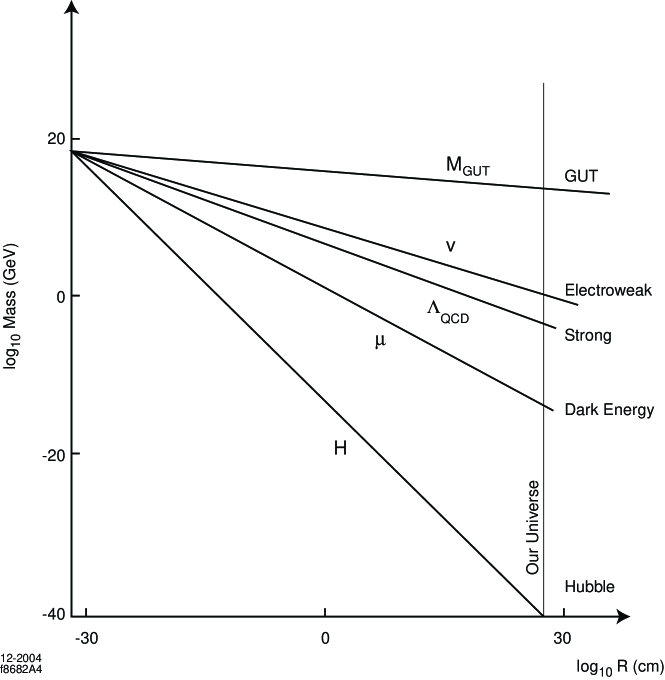
Figure 4: Assumed size dependence of standard model vacuum parameters.

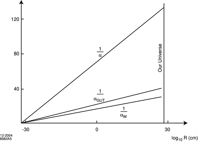
Figure 5: Size dependence of coupling constants.

The details of all this, including what to do with the remaining mass and mixing parameters of the standard model, are explored in the previous papers [5]. It is not our intention to retread all of this ground here, but only to highlight the main consequences of those investigations. In brief, they are that many properties of our universe, like the existence of chemistry and of recognizable nuclear forces and nuclear matter, are robust and can exist over a broad range of sizes. However, when one addresses the issue of the range of sizes over which life as we know it can be expected to exist, there are stronger constraints, well known to the anthropic community [13]. These constraints are sensitive to small quantities such as the pion to proton mass ratio, controlled by the masses of the up and down quarks, quantities which are in the several-MeV mass range. The size dependence of such quantities is harder to infer, because of the lack of good fundamental theory for those small numbers. But despite such uncertainty, it is still the case that there is a rather robust conclusion that can be made: the range of sizes over which life as we know it can exist is modest—no more than a factor two in either direction away from the size of our universe. The uncertainty in this estimate is considerable, but arguably less than an order of magnitude, And the origin of the most stringent constraint should not be surprising to those familiar with anthropic fine-tuning arguments. It is the triple-alpha process responsible for synthesis of carbon from helium in the interior of stars. There is a crucial resonance in carbon, with properties predicted in advance of its discovery. In particular the resonance has an excitation energy which is precisely what is needed to make the process go at the requisite rate, and which in our context has dependence on the ratio of pion to proton mass [5, 14].

5 Implications of the Scaling Hypothesis for the Hierarchy Problems

If the scaling hypothesis we have made were to deliver no insight into basic unsolved problems, it could well be argued that the above exercise is doomed to be inconsequential speculation. However, as we have already mentioned in the introduction, there are interesting implications for the hierarchy problems present in particle physics. The most quoted hierarchy problem is the disparity between the electroweak and Planck/GUT scales. But there are others, such as the small ratio of, say, the electron mass to the top quark mass. And of course the small value of the cosmological constant is another.

From the results of the previous section, these large numbers can be “understood”. Inspection of Fig. 4 shows that small universes, with sizes of order the GUT scale or smaller, do not have much if any hierarchy problem. Small universes are nontrivial, rather strongly coupled systems, and may well be much more commonplace than big universes. Indeed, if one tries to visualize the distribution in sizes of the universes comprising the ensemble we consider, and makes the rather weak assumption that the integral over sizes converges, then it seems natural to make the most probable size small, rather than large. Our own preference, based on intuition alone, is that the distribution be approximately power-law:

$$R\,\frac{dN}{dR}\sim pN_{\rm tot}\left(\frac{R_{\min}}{R}\right)^{p}\ .$$ (7)

Anthropic reasoning would suggest that the total number of universes in this distribution which are at least as large as our own should be large in comparison to unity. This means that if

$$R_{\min}\buildrel>\over{{}_{\sim}}M^{-1}_{\rm planck}\ ,$$ (8)

then the total number of universes in the ensemble should exceed

$$N_{\rm tot}\sim 10^{60p}\ .$$ (9)

This is large, but not off scale in comparison to other numbers which appear in cosmology, as long as $p$ has a reasonable value. Under these circumstances, habitable universes are rare, but not so rare as to be improbable.

Now let us return to the issue of the hierarchy problem. We have seen, given any size distribution which is qualitatively like the above example, that the typical, small universe has no hierarchy problem. Our universe is atypically large, and must be so because of the anthropic constraint that it be capable of supporting life as we know it. And because of the scaling of parameters, this implies that the hierarchies naturally exist in our universe. Again, we emphasize that this argument addresses all the hierarchies that are observed, not only the electroweak one, provided small parameters like electron and quark masses also flow to the Planck/GUT fixed point (not necessarily in a straight-line manner) for universes of small size. Of course, as mentioned in the introduction, this argument cannot really be regarded as a definitive solution to the hierarchy problems because it is contingent on the scaling hypothesis, which remains to be explained. But we do see that the problem has been recast. It is often the case in science that the recasting of a problem in different terms can be a key to its solution. So there is good reason to pursue further the consequences of what has been suggested above.

The restatement of the hierarchy problem is that the rationale for the behavior exhibited in Fig. 4 must be understood. Inspection of the figure shows that (by definition), the scaling behavior of the dark-energy scale is

$$\mu(R)\sim R^{-1/2}$$ (10)

while, to good accuracy, the behavior for the QCD scale is

$$\Lambda_{\rm QCD}(R)\sim R^{-1/3}\ .$$ (11)

The behavior for the electroweak scale is, to somewhat lesser accuracy,

$$v(R)\sim R^{-1/4}\ .$$ (12)

Therefore the recasting of the hierarchy problem reduces to the understanding of the origin of the “critical exponents” of 1/3 for QCD and of 1/4 for the electroweak theory. The large numbers are gone, but mystery remains. In the next section we shall explore a possible attack on the QCD exponent of 1/3. We have nothing useful to say here, however, about the electroweak 1/4 [15].

6 The Critical Exponent of QCD

The observation that the QCD scale is a factor 20/60 = 1/3 of the way (on a logarithmic scale) between the Planck scale of $10^{-33}$ cm and the cosmological scale of $10^{28}$ cm goes back 35 years to Zeldovich [16], and has been occasionally rediscovered since then [17]. We here approach the problem from a perhaps surprising starting point, namely the thermodynamic description of horizons in general relativity. The starting point lies in work of Padmanabhan [18], who has found a simple connection between the structure of the Einstein-Hilbert Lagrangian and the thermodynamic description of horizons a la Bekenstein and Hawking.

Padmanabhan begins by considering metrics of Schwarzschild type:

$$ds^{2}=[1-u(r)]^{2}dt^{2}+[1-u(r)]^{-2}dr^{2}+r^{2}d\theta^{2}+r^{2}\sin\theta\,d\phi^{2}$$ (13)

and finds that the Lagrangian $L$, as a functional of $u$, is a perfect derivative

$$L=\frac{M^{2}_{pl}}{16\pi}\int^{r}_{0}d^{3}x\,R(u)=\frac{M^{2}_{pl}}{4}\int^{r}_{0}dr\frac{\partial}{\partial r}\left[r^{2}\,\frac{du}{dr}-2ru\right]\ .$$ (14)

If one evaluates the resulting surface integral at a horizon $R$, where $u(R)=1$, and where the surface gravity at the horizon

$$u^{\prime}(R)=4\pi T$$ (15)

can be identified with the Bekenstein-Hawking temperature $T$ as indicated, one finds

$$L=\frac{1}{4}(4\pi R^{2}M^{2}_{pl}T)-\frac{1}{2}M^{2}_{pl}R=TS-M\ .$$ (16)

We see that the two terms can be identified as the entropy term and energy, or mass, term respectively in the “first law of black-hole thermodynamics”, with the correct numerical coefficients [19]. This can be no accident, and undoubtedly there is much more to be understood here. Here we will only pursue one general consequence of Padmanabhan’s construction. Let us apply it to static deSitter space, which in fact is the spacetime appropriate to our cosmological future. In that case

$$u=\frac{r^{2}}{R^{2}}=H^{2}r^{2}\ .$$ (17)

We see from Eq. (14) that the Bekenstein-Hawking entropy term, just like the accompanying energy or mass term, is cast as an integral over a constant density. This is somewhat surprising, since typical intuition regarding horizon entropy suggests a visualization where the entropy is contributed by a summation over bits of information residing on the horizon surface, of order one bit per Planck area, rather than a summation of bits within the bulk volume. What is instead suggested is that there are also bits in the bulk, in one-to-one correspondence with the bits on the surface. So it is suggestive to identify each bit residing in the bulk with a bit residing on the surface by connecting them with a “string”. With this construction we arrive at a picture that the objects to be counted in building up the Bekenstein-Hawking entropy are the strings themselves, including possible structures at the ends. In this way there is no contradiction between the two ways of viewing the origin of the entropy. Evidently a topological origin of this structure is suggested. The string might be a Dirac string, or alternatively some kind of vortex structure containing physical, as opposed to gauge, degrees of freedom. The end of the string residing at the horizon will find itself in an ultraviolet regime, so that its internal structure may reflect GUT symmetry such as SU(5), while its extension into the bulk may undergo GUT symmetry breaking, leaving a net QCD structure behind.

The connection with the QCD scaling exponent comes from estimating the density of the entropy in the bulk. It is simply

$$s=\frac{S}{V}=\frac{\frac{1}{4}(4\pi R^{2})M^{2}_{pl}}{\frac{4}{3}\pi R^{3}}=\frac{3M^{2}_{pl}}{4R}\ .$$ (18)

Using

$$\lim_{t\rightarrow\infty}H(t)=H=0.7\times 10^{-10}\ {\rm yr}^{-1}$$ (19)

we obtain

$$s\cong(0.3\ fm^{-1})^{3}\sim(\Lambda_{\rm QCD}/3)^{3}$$ (20)

which is quite close to the observed vacuum scale of QCD. Note that the dependence of the entropy density on the size of the universe in Eq. (18), here represented by the radius $R=H^{-1}$ of the deSitter horizon, does agree with the QCD scaling exponent of 1/3. It is also interesting that the energy per bit $\epsilon$ is simply the Bekenstein-Hawking temperature:

$$\epsilon=\frac{M}{N}=\frac{1}{2\pi R}=T\ .$$ (21)

Again, we have not solved our problems, but recast them in a different form. It is now rephrased as an exercise in understanding how nonperturbative structures of the QCD vacuum can be identified with vacuum structures in cosmology, in particular structures associated with cosmological horizons. We do not offer any clear answer here. Our preferred hypothesis is that the entropy is to be identified with the “topological charge” $N$ of the wave functional of the QCD vacuum.

Recall that the CP violating term in the QCD action

$$\int L\,dt=\frac{\theta}{24\pi^{2}}\int d^{4}xE\cdot B=\theta\int d^{4}x\frac{\partial K_{\mu}}{\partial x_{\mu}}=\theta\int dt\frac{\partial N}{\partial t}$$ (22)

is expressible in terms of the time derivative of the “topological charge” $N$

$$N=\int d^{3}x\ K_{0}(x,t)$$ (23)

which is the quantity canonically conjugate to the $\theta$ parameter of QCD. If $N$ indeed has a huge expectation value,

$$\left\langle{N}\right\rangle\sim 10^{120}$$ (24)

then all the instanton-induced transitions throughout the history of the universe will not be enough to change it significantly. To see this assume one transition per cubic fermi per fermi of time. It follows that

$$(\Delta N)^{2}\sim(10^{28}\rm{cm}/10^{-13}{\rm cm})^{3}\times(10^{10}{\rm yr}/10^{-23}\sec)\sim 10^{160}\ll\left\langle{N}\right\rangle^{2}\ .$$ (25)

The large value of $N$ allows both it and its canonically conjugate $\theta$ to be considered as classical variables. This in turn may eventually shed some light on the strong CP problem. But further investigation in this direction is beyond the scope of this note.

In any case, the bottom line of this discussion is that the vacuum structure of QCD may be strongly linked to the large scale structures in cosmology, in particular horizon structures. In the context of string-theory investigations such as AdS/CFT and its ramifications, this may not be too surprising a conclusion.

7 The Inflationary Universe as a Separate Universe

We now turn to another possible ramification of the scaling idea, one which may have too many, instead of too few experimental consequences. We have thus far defined a universe by its size, as determined by the value of the dark energy (or equivalently Hubble) scale at late times. However in our own universe the inflationary epoch contains a different, much larger dark-energy (and Hubble) scale than at late times. Might it not therefore be appropriate to subdivide our universe into two distinct universes? The inflationary universe would be characterized not only by a different dark-energy scale than the subsequent big-bang universe, but also by different standard model parameters. Indeed, examination of Fig. 4 shows that for universes of size $10^{5}$ or $10^{6}$ times larger than the Planck size, the QCD scale and the electroweak scale are in the neighborhood of the GUT scale—if anything on the high side. So a credible and simple candidate scenario is that for this small inflationary universe the electroweak and QCD interactions are in fact already unified, and that the scale of their vacuum parameters might be appropriate for identification with the inflationary dark energy scale itself! What has to happen at the end of inflation, the so-called “reheating” period, is in this picture quite profound—a real change of vacuum phase, complete with a new set of standard model parameters and with possibly a new, distinct pattern of symmetry breaking. And as we shall mention at the end of this section, the nature of the reheating transition from the inflationary universe to the big-bang universe might be even more profound, involving the basic structure of quantum theory itself.

However, before considering such things, we can reverse the procedure and consider the role of the inflaton field, both in the small, inflationary universe, where it plays its traditional role, and in the late, big-bang universe, where the parameter scaling will lead to a different role. There are a large variety of inflaton models to consider. But in this brief introductory exploration of issues, we restrict our attention to a typical hybrid-inflation model in order to get an idea of what is involved. The inflaton potential is taken to be of a small scale, much less than what accounts for the bulk of the inflationary dark energy. The form we take is “natural”, i.e. pseudo-Goldstone:

$$V(\phi)\sim m^{4}\cos(\phi/F)\ .$$ (26)

How this choice is fit to data on cosmic microwave background fluctuations is a straightforward application of standard inflation theory. The result is that the typical magnitude of the inflaton field is of order $F$ in the above equation, with $F$ naturally taken to be of order the GUT scale. Then the magnitude of the inflaton “dark-energy” scale $m$, determined by the strength of the inflaton potential, must be two to three factors of ten smaller, in order to account correctly for the small size of the primordial perturbations. If we then extrapolate this potential back to our universe using the appropriate scaling law, as shown in Fig. 6, we see that the strength of the potential for our universe is extraordinarily small—the scale of the inflaton dark energy will be 40 or 50 powers of ten smaller than the Planck scale (Fig. 7). We know of no candidate beyond-the-standard-model field which might be identified with this inflaton.

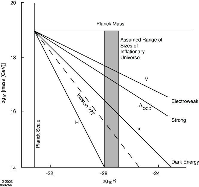
Figure 6: Size dependence of vacuum parameters for small universes.

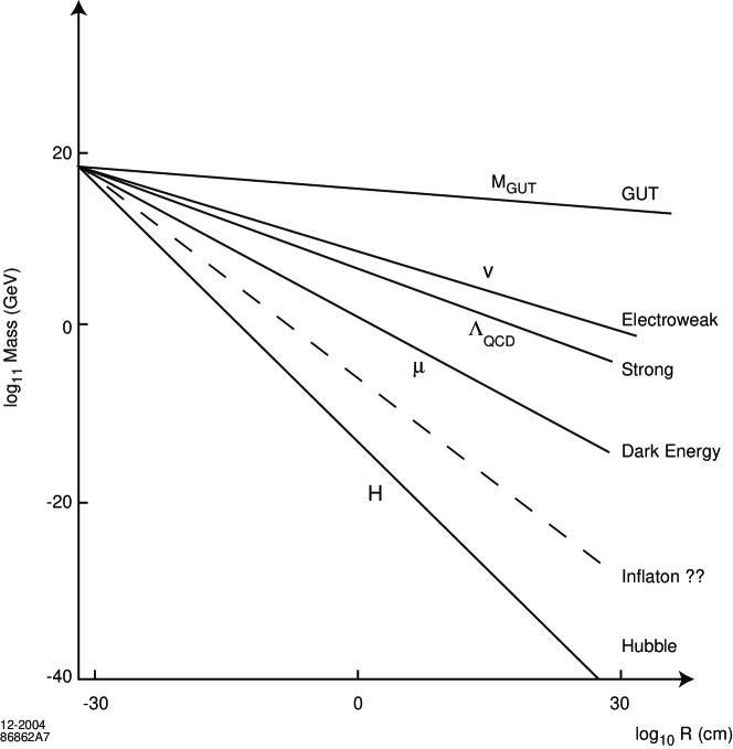
Figure 7: Size dependence of vacuum parameters with conjectured inflaton dark energy scale included.

This kind of exercise can be repeated for the whole array of inflaton models, although no attempt will be made here to do so. We only emphasize that there are possible observational implications for these exercises.

Before leaving this section, we will elaborate on the comment made above regarding the possibility that foundations of quantum mechanics might become involved in this two-universe scenario. The reason originates in the observation, made already in earlier references [5], that the scaling behavior of the couplings with size that we have described can be recast as an overall rescaling of the standard-model Lagrangian density. In brief, this occurs as follows. Write the Lagrangian schematically as follows:

$$\mathcal{L}=F^{2}+\overline{\psi}(\partial-eA)\psi+\phi(\partial-eA)^{2}\phi+e\overline{\psi}\psi\phi+\lambda\phi^{4}+m^{2}\phi^{2}\ .$$ (27)

The terms, in order of appearance, represent (1) the gauge field kinetic energies, (2) the quark and lepton kinetic energies, (3) the Higgs-field kinetic energies, (4) the Higgs Yukawa couplings, (5) the quartic Higgs self-couplings, and (6) the Higgs mass term. The quantity $e$ represents any of the gauge or Higgs Yukawa couplings, all of which are assumed to have the property that $e^{-2}$ scales logarithmically with the size of the universe, in accordance with the behavior shown in Fig. 5. The natural assumption that this behavior will also be true for $\lambda^{-1}$, the inverse of the quartic Higgs coupling, has also been made. Then under the field redefinitions

$$eA\rightarrow A\qquad e\phi\rightarrow\phi\qquad e\psi\rightarrow\psi$$ (28)

we see that, except for the Higgs mass term, the dependence on scale factors out, with an overall factor $e^{-2}$ multiplying the Lagrangian density. Its scale dependence is simply

$$\mathcal{L}\sim e^{-2}\mathcal{L}_{0}\sim(\log R)\mathcal{L}_{0}\ .$$ (29)

But this is tantamount to a scale dependence of the Planck constant,

$$\hbar\sim(\log R)^{-1}$$ (30)

because its inverse is also an overall multiplier of the action. With this interpretation, the Planck constant is (logarithmically) large for small universes and small for large universes.

We do not know whether the above feature should be regarded as a mere curiosity or as an indication that there is something in the structure of quantum theory that is connected to the large-scale geometry of the universe. Were the latter to be the case, then the big-bang ignition, or “reheating”, transition from the inflationary universe to the radiation-dominated universe would be of paramount importance to fully understand. Within that dynamics would lie some of the deepest secrets of the theory that could possibly be revealed to us, because in that transition the value of the Planck constant, as well as the values of the vacuum parameters of the theory, would change discontinuously. It would also be imperative in that scenario to entertain the possibility of the Planck scale and/or the speed of light also to abruptly change during big-bang ignition.

8 The Beginning of Inflation

In Section 2 we used Fig. 2 describing the “universe for dummies” as evidence that its global spacetime architecture was controlled by one large number of order $10^{30}$, the ratio of dark energy scale to Planck scale. One of the curiosities of that point of view is that the inflationary epoch, characterized by large energy and small distance scales, when initiated at the initial time we chose, is also characterized by the same number, even though the small dark energy we observe today has not yet entered the picture. It is arguable that this situation was created by construction. We demanded that the starting time chosen for evolution of our universe be identified, at least approximately, with the time at which the size of the future event horizon is comparable to the inverse Hubble scale. But the future event horizon was constructed with knowledge of the properties of the universe at future times, times when the cosmological constant is in fact present.

Nevertheless, whatever one’s point of view, there remains the problem of how the universe during inflation, where only large energy scales and small distances dominate, manages to evolve during the big-bang ignition phase into a universe containing the tiny present-day cosmological constant. It would seem that the curiosity described in the preceding paragraph might present a clue. One element of that clue will be the assumption that inflation really does commence at the landmark time which we have chosen as the starting time of our universe-in-a-box. And the idea that we pursue is that at this initial time there is not only dark energy present but also radiation, and perhaps ordinary matter as well, with comparable energy densities. In other words, the initial state of the inflationary phase is qualitatively not so different from the state of the universe right now. And we must remember that the universe now is also about to enter an inflationary phase.

The evolution of the “universe for dummies” from this starting point is then straightforward: the dark energy almost immediately dominates the Hubble parameter, and the radiation energy density diminishes as $a^{-4}$, while the matter energy density diminishes as $a^{-3}$. The logarithm of these energy densities are plotted in Fig. 8 versus the logarithm of the scale factor. This plot is essentially the same as Fig. 4 turned on its side, because energy densities are related to the Hubble scale in a direct way through the FRW equation.

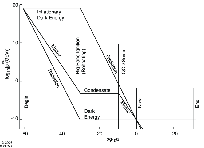
Figure 8: Conjectured evolution of energy densities in the “universe for dummies”.

We see that if the radiation component we have introduced is assumed to condense into dark energy at the end of inflation, then the magnitude of the dark energy comes out correctly. The fate of the matter component is also interesting. If it also condenses into dark energy at the end of inflation, there will be far too much of it nowadays. To account approximately for the amount of dark matter present nowadays, this dark energy must melt into “matter” when the Hubble parameter is 40 powers of ten larger than the Planck scale, corresponding to the cosmic background temperature being 20 powers of ten less than the Planck temperature. But this is just the temperature scale to be associated with QCD. And the behavior of this dark energy conversion is just what happens if dark matter is composed of axions. At the beginning of the big bang the axions behave as a condensate, but in the neighborhood of the QCD transition the condensate undergoes quantum fluctuations, and thereafter those fluctuations behave as a nonrelativistic noninteracting gas in thermal equilibrium.

While this scenario has a certain tidiness, and might provide a glimpse into the prehistory of the evolution of both the dark matter and dark energy seen nowadays, it is an idealized one, constructed in the context of the “universe for dummies”. It then becomes a serious and very interesting issue as to whether the scenario can remain viable when all the real life complications and details present in our universe are restored. This is very much a numbers game, and a very interesting one to play. The net result is that the scenario without the dark-matter component appears to be quite robust (Fig. 9). But the inclusion of the dark matter into the game is not as easy. It seems to require an assumption that the transition from the end of inflation to the beginning of radiation-dominated big bang is not instantaneous. The duration of this “reheating” epoch should allow the scale factor $a(t)$ to increase by a factor of order a thousand. This is illustrated in Fig. 10.

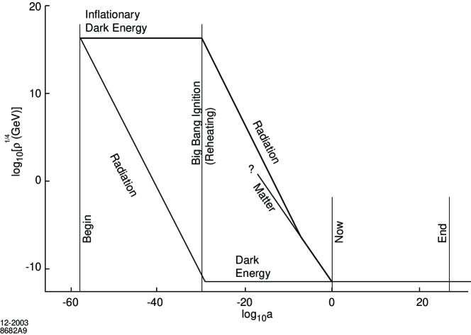
Figure 9: Conjectured evolution of energy densities for the real universe, without consideration of dark matter.

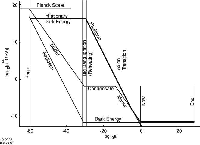
Figure 10: Conjectured evolution of energy densities for the real universe, with an attempted incorporation of dark energy.

The above scenarios suggest a kind of self-similarity in the evolution of the universe: the beginning of inflation is analogous to the present epoch, when dark energy begins to dominate over matter and radiation. And our future might be similar to the inflationary epoch, perhaps terminated by another abrupt transition to a big-bang universe containing an even smaller cosmological constant. And there might be an epoch prior to what we have called the beginning of inflation, again of big-bang character, and taking one back to a truly Planckian origin. It might also be interesting to try to combine this scenario with the ideas of the preceding section, where each such epoch is not only self-similar but also possesses a different set of standard model parameters. However, the combining of the speculations in this section with those in the previous section may not be mandatory.

9 Concluding Remarks

One of the main purposes of this paper has been to cast multiverse ideology in as bottoms-up, phenomenologically driven a way as possible. This is expedited by the definition, by construction, of a universe which is big enough to contain essentially all of presently conceivable phenomenology, but small enough to exclude most of the commonplace and extravagant theoretical speculations enveloping the subject. The experimental accuracy of the cosmological principle, within the portion of the universe that we have observed, then allows a very credible extrapolation to relatively nearby regions of spacetime, where an ensemble of such universes can be similarly constructed.

Going only this far seems to us a quite conservative procedure, at least by contemporary standards of theoretical cosmology. More interesting is the next step, which posits that the ensemble can be generalized to include more distant members, of similar FRW spacetime structure. But these members are assumed to have different standard model parameters, in particular different cosmological constants. In the context of present activity in string theory, this step is also not very radical. However, acceptance of this step then invites introduction of anthropic reasoning, especially with respect to the role of the cosmological constant as an anthropically determined parameter.

At this point the level of controversy increases, because as soon as anthropic arguments are introduced, it is hard to determine when to stop. If the cosmological constant is determined only anthropically, what about all the other standard model parameters? Do they not also serve as labels for the gigantic number of vacuua in the string theory landscape? And if they are all anthropically determined, where does that leave, say, the future program of particle physics? The original dreams of a final theory, as visualized two decades ago [20], lay at the opposite extreme, with specific and naturalistic explanations of those parameters expected to be provided by the future theory. Instead they may be only constrained by the fact that we exist in the universe to observe them [6].

It is not for us to dictate the answer. Maybe all the parameters are anthropic, in which case the scientific method becomes relatively impotent. Maybe none of them are, despite the evidence of fine-tuning of parameters which has been uncovered and studied by the anthropic community over the last fifty years [13]. And maybe the answer lies in between the extremes.

It is this latter hypothesis which we have chosen in this paper. It is implemented by the presumption that, within the ensemble of universes we have constructed, at least the principal parameters of the standard model are strongly correlated with the value of the cosmological constant. We have also proposed a specific form of the correlation. This last step has been greeted with much skepticism, most often in a completely dismissive way. Perhaps this occurs because of the lack of any overarching theoretical ideology to motivate the scaling hypothesis. In defense, we argue from experience in searching for alternatives that the scaling hypothesis stands out in its simplicity and robustness [21]. Dreamers of final theories would naturally expect most standard model parameters to be correlated with each other, because a good theory should have very few independent parameters. But it is a priori unlikely that the correlations take a simple form, so simple that the right answer can be correctly guessed. We work from a naive sense of optimism at this point, but are rather convinced that if there is a simple form of the correlation, the proposed correlation is likely to be, at the least, very similar to the correct one.

Support for this point of view comes from the output, which provides some understanding of the hierarchy problems of particle physics. As we discussed, the hierarchy problem is traded in for the problem of understanding certain “critical exponents” such as 1/3 for QCD and 1/4 for the electroweak sector. An attempt at understanding the 1/3 of QCD was sketched in Section 6.

Here we only point out that that attempt, along with other spinoff ideas in the subsequent two sections, are not at all abstract. They deal with the understanding of very real issues existing within our own universe, such as the structure of the QCD vacuum, and the nature of the big-bang ignition (“reheating”) epoch of our universe. It is evidence that consideration of multiple universes may conceivably help, at a quite phenomenological level, in uncovering the nature of physical processes in our own universe.

Appendix A: Cosmology 101

We here record equations used in constructing the figures in the text. We do assume familiarity with the physics of big-bang cosmology, as described in standard texts.

The FRW equation is

$$H^{2}(t)=\frac{8\pi}{3M^{2}_{pl}}\,\rho(t)$$ (A.1)

with $\rho(t)$ the energy density of sources, and the Hubble expansion parameter

$$H(t)=\frac{\dot{a}(t)}{a(t)}\ .$$ (A.2)

The equation of state of the source of energy must be specified. Generically, one writes

$$p=\omega\rho$$ (A.3)

with $\omega=0,\ \frac{1}{3},$ and $-1$ for matter, radiation, and dark energy, respectively. Then energy-momentum conservation demands

$$d(\rho a^{3})=-p\,d(a^{3})\ .$$ (A.4)

Solution of these equations for the scale factor yields

$$a(t)\sim\left\{\begin{array}[]{l@{\qquad}l}t^{1/2}&{\rm Radiation}\\ t^{2/3}&{\rm Matter}\\ e^{Ht}&{\rm Dark\ energy}\end{array}\right.$$ (A.5)

The behavior of $H$ versus $a$ is then

$$H(a)\sim\left\{\begin{array}[]{l@{\qquad}l}a^{-2}&{\rm Radiation}\\ a^{-3/2}&{\rm Matter}\\ {\rm constant}&{\rm Dark\ energy}\end{array}\right.\ .$$ (A.6)

These results are readily checked by substitution in Eqs. (A.1) and (A.2). In Fig. 4 we assume abrupt transitions between the various epochs shown. At the transitions both $H$ and $a$ must be continuous. From the equation of state for radiation we readily deduce that the mean wavenumber $k$ of photons in the cosmic microwave background scales as

$$k\sim a^{-1}\ ,$$ (A.7)

whether or not the photons are in thermal equilibrium. When thermal equilibrium applies, evidently $k$ is a measure of temperature.

One important simplification we have made occurs in the radiation-dominated epoch. The equation of state is, expressed in terms of temperature,

$$\rho=g(T)\,T^{4}$$ (A.8)

and the density of states factor $g(T)$ decreases by more than an order of magnitude during expansion. This changes slightly the plotted curves. But on the scale shown, it is scarcely noticeable.

In the deSitter epoch in our future, Eq. (6) for the future event horizon simplifies to

$$E(t)=H^{-1}\ ,$$ (A.9)

while in the matter and radiation-dominated eras,

$$E(t)\approx a(t)\int^{\infty}_{0}\frac{dt^{\prime}}{a(t^{\prime})}=a(t)\,\eta_{0}\ .$$ (A.10)

In that epoch, the slope of the curve for log $E(t)$ versus log$\,a$ is $+1$, as shown in Figs. 2 and 3.

References

- [1] M. Rees, “Our Cosmic Habitat” (Princeton Univ. Press, Princeton NJ, 2001); “Just Six Numbers” (Basic Books, NY, 2000); astro-ph/0401424.
- [2] M. Fonstad, W. Pugatch, and B. Vogt, Annals of Improvable Research 9, no. 3, 16 (2003).
- [3] This conclusion may still be reached by a modern family, with small children, while driving across that great state.
- [4] For a splendidly extravagant example, see M. Tegmark (astro-ph/0302131), “Science and Ultimate Reality: From Quantum to Cosmos”, ed. J. Barrow, P. Davies, and C. Harper, Cambridge Univ. Press (2003).
- [5] J. Bjorken (hep-th/0210202), Phys. Rev. D 67, 043508 (2003); (hep-th/0103349), Phys. Rev. D 64, 85008 (2001).
- [6] L. Susskind, hep-th/0302219, and references therein.
- [7] D. Brownlee and P. Ward, “Rare Earth” (Copernicus, Springer-Verlag, New York NY, 1999).
- [8] For recent attempts, see C. Lineweaver, Y. Fenner, and B. Gibson, astro-ph/0401024; D. Underwood, B. Jones, and P. Sleep, astro-ph/0312522, and references therein.
- [9] E. Kolb and M. Turner, “The Early Universe” (Perseus, Cambridge MA, 1990).
- [10] A. Linde; Phys. Rev. D 49, 748 (1994). For reviews of inflationary models, see A. Riotto, hep-ph/0210162; S. Tsujikawa, hep-ph/0304257.
- [11] S. Hawking and G. Ellis, “The Large Scale Structure of Spacetime” Cambridge Univ. Press (1973).
- [12] See for example, L. Dyson, M. Kleban, and L. Susskind, hep-th/0208013; T. Banks, astro-ph/0305037, and references therein.
- [13] J. Barrow and F. Tipler, “The Anthropic Cosmological Principle”, Clarendon Press, Oxford (1986).
- [14] F. Hoyle, D. Dunbar, W. Wenzel, and W. Whaling, Phys. Rev. 92, 1095 (1953); M. Livio, D. Hollowell, A. Weiss, and J. Truran, Nature 340, 281 (1989); H. Oberhummer, R. Pichler, and A. Csoto, nucl-th/9810057.
- [15] See for example, N. Arkani-Hamed, L. Hall, C. Kolda, H. Murayama, astro-ph/0005111; T. Banks, hep-th/0206117.
- [16] I. Zeldovich, JETP Lett. 16, 316 (1967); Soviet Physics Uspekhi 11, 381 (1968).
- [17] R. Schutzhold, gr-qc/0204018; S. Carniero, gr-qc/0305081.
- [18] T. Padmanabhan, gr-qc/0205090; Gen. Rel. Grav. 34, 2029; gr-qc/0311036 and other references therein.
- [19] We note that the relation is true for both a Schwarzschild black hole or for the total dark energy inside a static deSitter horizon.
- [20] S. Weinberg, “Dreams of a Final Theory”, Pantheon, Random House, New York NY, 1992; B. Greene, “The Elegant Universe”, Norton, New York NY, 1999.
- [21] On the other hand, it may just be the author’s attempt to relive his youth. See J. Bjorken, “In Conclusion”, World Scientific, Singapore (2003).