Lightcurve Classification in Massive Variability Surveys II: Transients towards the Large Magellanic Cloud.

Abstract

Automatic classification of variability is now possible with tools like neural networks. Here, we present two neural networks for the identification of microlensing events – the first discriminates against variable stars and the second against supernovae. The inputs to the networks include parameters describing the shape and the size of the lightcurve, together with colour of the event. The network computes the posterior probability of microlensing, together with an estimate of the likely error. An algorithm is devised for direct calculation of the microlensing rate from the output of the neural networks. We present a new analysis of the microlensing candidates towards the Large Magellanic Cloud (LMC). The neural networks confirm the microlensing nature of only 7 of the possible 17 events identified by the MACHO experiment. This suggests that earlier estimates of the microlensing optical depth towards the LMC may have been overestimated. A smaller number of events is consistent with the assumption that all the microlensing events are caused by the known stellar populations in the outer Galaxy/LMC.

1 Introduction

Microlensing is rare and out-numbered by stellar variability by at least a factor of ten thousand. Despite this, the selection of microlensing candidates in variability surveys seems straightforward at an optimistic first glance. Unlike almost all forms of stellar variability, microlensing is achromatic, time-symmetric and does not repeat. The theoretical form of the microlensing lightcurve is well-known (e.g., Paczyński 1986) and so events can seemingly be selected by their goodness-of-fit in two passbands.

In practice, the selection of candidates is fraught with difficulties. The lightcurves are usually sparsely sampled and noisy – for example, the median seeing at the site of one of the most prominent microlensing experiment (MACHO) is $\sim 2.0^{\prime\prime}$. More awkwardly still, the clear-cut set of characteristics of microlensing only holds good in the simplest case of an isolated point-mass lensing a point-source. In fact, microlensing lightcurves may show colour variations because of blending (e.g., Di Stefano & Esin 1995). They may show substantial deviations from time-symmetry because of parallax or xallarap effects (Dominik 1998; Mao et al. 2002) or because the lens is a binary star (e.g., Mao & Paczyński 1991; An et al. 2004).

As a consequence, the results of the microlensing experiments towards the Magellanic Clouds by the MACHO and EROS collaborations remain controversial (e.g., Evans 2002). From 5.7 years of data, the MACHO collaboration identified between 13 and 17 candidates towards the Large Magellanic Cloud (LMC) and reckoned that the optical depth is $1.2^{+0.4}_{-0.3}\times 10^{-7}$ (Alcock et al. 2000). The first set of 13 events comprises the most convincing candidates, whilst the second set of 17 candidates includes an additional 4 events less firmly established. This is in astonishing contrast to the results reported by the EROS collaboration, who found just 3 events towards the LMC (Lasserre et al. 2000). The two experiments are not directly comparable as EROS monitor a wider solid angle of less crowded fields than do MACHO. Even though EROS do not analyze their data in terms of optical depth, it is clear that the results point to a lower value than that claimed by MACHO. Tellingly, a similar discord prevails in the results towards the Galactic Centre; MACHO (Alcock et al. 1997) recorded that the microlensing optical depth to the red clump stars as $3.9^{+1.8}_{-1.2}\times 10^{-6}$, while EROS (Afonso et al. 2003b) found a value of $0.94\pm 0.26\times 10^{-6}$ at almost the same location. These discrepancies strongly suggest that the systematic effects in the experiments are not yet fully understood, with candidate selection fingered as the most likely culprit.

All this motivated Belokurov, Evans & Le Du (2003) to introduce neural networks as an automatic way of classifying lightcurve shapes in massive variability surveys. They constructed a working neural network for identification of microlensing events and applied it to microlensing data towards the Galactic Centre. In this paper, the ideas and methods of analysis are extended to the variability datasets taken towards the LMC. This is a harder problem, as the source stars are fainter and hence the microlensing events less clear-cut. A particular difficulty already identified by Alcock et al. (2000) is the contamination of samples of microlensing events by supernovae in distant galaxies behind the LMC.

Variable Type	Specific Examples	Number
Eruptive	Pre-Main Sequence, R Corona Borealis stars	34
Pulsating	RV Tauris, Mira, Semi-Regular variables	595
	Cepheids	372
	Bumpers	300
Cataclysmic	Supernovae, novae, recurrent novae	45
Eclipsing		135
MACHO samples		531
Microlensing		1500

Table 1: Composition of the training set. There are 1500 examples of microlensing and 2014 examples of other classes of lightcurves. The sources for the data are reported in the main text.

2 Lightcurve classification with neural networks

Let us briefly review the main stages of a classification routine with neural networks (see Bishop 1995 for more details). As a first step, the lightcurves are pre-processed with the primary goal of reducing the amount of data to be examined. Features can be extracted automatically, for example, with the help of spectral analysis or principle component analysis. Alternatively, we can try to incorporate a priori information and use only those features that are believed to quantify characteristic properties of the lightcurve, such as shape, periodicity or colour. These features are then normalized to provide inputs for the neural network. An optimum choice of inputs is the key to success.

The next stage involves choosing a particular architecture for the neural network (such as the number of hidden units or layers) and training the network on the set of previously classified patterns of inputs $x_{i}$. The logistic activation function is used and the output neuron takes values in the range between 0 and 1. Thus, the output $y$ models the posterior probability of the variability classes (see e.g., Bishop 1995 or Belokurov et al. 2003). Training is performed by minimizing the error function, which consists of the standard cross-entropy term and the weight decay term $\alpha\sum_{i}w^{2}_{i}$, where the sum runs over all weights $w_{i}$. Adjusting a hyper-parameter $\alpha$ enables one to control the magnitude of weights and hence to minimise any over-fitting. This can be done automatically during training. This differs from the procedure used in Belokurov et al. (2003), as no validation set is required and the whole of the available data can be used as a training set. Further reduction of the variance in network predictions can be achieved by using a committee of networks. A very inexpensive but efficient way of introducing the committee involves simply taking the output of the committee to be the average of the outputs of the individual networks. The members of the committee are competing solutions of the classification problem, which occurred as a result of starting the search in the parameter space from different initial weights. It is also beneficial to combine networks with different numbers of neurons in the hidden layer.

Finally, each new lightcurve has to be pre-processed and the features extracted have to be fed to the trained network, which is defined by the most probable parameter vector of weights $w_{\rm MP}$. The output of the network is $P(C_{1}|x,w)$, the probability that the lightcurve belongs to the class $C_{1}$ or microlensing given the inputs $x$ and the weights $w$. The output can therefore then be used to make a decision as to which class the current datum belongs. Usually, the lightcurve is assigned to the class for which the posterior probability is largest. For a two-class problem with equal priors this implies a formal decision boundary at $y=0.5$. Although usually different classes do have roughly equal prior probabilities in the training set, in reality this need not be the case. We can correct for this by adjusting the outputs of the trained network using the ratios of prior probabilities for each class. As we show in Appendix A, this can be exploited to calculate the microlensing rate directly from the neural network outputs. We can also allow for this by moving the decision boundary and classifying objects as microlensing only if the probability exceeds some higher threshold than the formal decision boundary.

Once we have transformed the new input pattern into the posterior probability, it is important to have an estimate of the error in the output. The error arises through variance and through undersampling in the parameter space during training. The variance part of the output error is easiest to deal with. It can be approximated by taking the standard deviation of the output of a committee of neural networks. The second part of the output error is more awkward, but can can be approximated by a method originated by MacKay (1992b), which we now explain.

There will always be regions in input space with low training data density. Typically the network with parameters $w_{\rm MP}$ will give over-confident predictions in such regions. A representative output then will be an output averaged over the distribution of network weights, namely

$$P(C_{1}|x,D)=\int P(C_{1}|x,w)p(w|D)dw.$$ (1)

Here, $C_{1}$ is the class (in our case, microlensing), $x$ denotes the inputs and $D$ the data in the training set. This integration cannot be performed analytically, but there is a simple approximation, namely

$$P(C_{1}|x,D)\approx f(k(s)a_{\rm MP}),\qquad k(s)=\left(1+\frac{\pi s^{2}}{8}\right)^{-1/2}.$$ (2)

Here, $f$ is the activation function, $s$ is the network variance and $a_{\rm MP}$ is the activation of the output neuron given the most probable distribution of weights (the one that is found during network training). The network variance is calculated using the methods of Section 10.3 of Bishop (1995). It can be shown that this marginalized or moderated prediction always has a value closer to 0.5 (the formal decision boundary in two-class problems) than the most probable one. Marginalization always drives the output closer to the formal decision boundary.

When any network is applied to real data after training, it is confronted with more complex light curves which inevitably extend beyond the data domain encountered during training. We caution that neural networks sometimes classify these in an unpredictable manner, as this amounts to an extrapolation of the decision boundaries. Our use of marginalized or moderated output guards against this, as unexpected or unpredicted patterns are then driven back to the formal decision boundary.

3 A CASCADE OF NETWORKS

Neural networks can be arranged sequentially in a cascade to perform complicated pattern recognition tasks. Here, the lightcurve data are examined first with neural networks which eliminate the contaminating variable stars. Then, lightcurves successfully passing this first stage are analysed anew with neural networks which eliminate contaminating supernovae. Excellent microlensing candidates must pass both stages.

3.1 A Network to remove the Variable Stars

Figure 1: The standard cross-entropy error plotted against the number of neurons in the hidden layer for the training set and the test set. This begins to flatten for the test set data around 6 or 7 neurons.

Figure 2: The false positive and false negative rates for single passband data when the committee of neural networks is applied to the test set. The horizontal axis is the network output. For the false negatives, the vertical axis is number of misclassified microlensing lightcurves expressed as a percentage of the total number of microlensing lightcurves. The solid line applies to the raw data without any cleaning. The dotted line corresponds to processing only lightcurves with at least 5 datapoint with signal to noise greater than 5 during the Einstein diameter crossing time. For the false negatives, the vertical axis is number of non-microlensing lightcurves misclassified as microlensing expressed as a percentage of the total number of non-microlensing lightcurves. The solid line applies to the raw data, while the dotted line corresponds to taking the maximum of the output for the raw and the cleaned lightcurves.

Figure 3: The locations of $\approx 22000$ MACHO lightcurves as given by the outputs of the committee $y_{R}$ and $y_{B}$ on processing the red data and the blue data respectively. These include the 29 lightcurves that passed the loose selection of Alcock et al (2000), together with $\sim 1000$ lightcurves in the vicinity of each candidate. Each point gives the maximum of the moderated output for the raw and the cleaned data, with the error bar giving the network scatter. A large open circles around a point indicates that it lies above the decision boundary ($y_{R}>0.87$ and $y_{B}>0.87$). Filled black dots represent the 29 lightcurves selected by Alcock et al. (2000), while all other lightcurves are represented by open grey dots.

Figure 4: The lightcurve of one of the false positives. This is close to the noise/microlensing border in parameter space.

To eliminate the variable stars, we use the techniques developed in Belokurov et al. (2003), but we make some modifications to the training procedures. The training set contains 3513 patterns, 1500 of which are derived from simulated microlensing lightcurves. These events are generated by randomly choosing an impact parameter, an Einstein crossing time between 7 days and 365 days and a time when the event reaches maximum. Random Gaussian noise is added to all the lightcurves and the experimental sampling is used. Only those events that have 3 or more datapoints during the event with a signal-to-noise greater than 5 are included in the training set. The remaining 2014 lightcurves in the training set are broken down according to Table 1. The sources of many of the variable star lightcurves, such as Miras, novae and eclipsing variables, are derived from the long data sequences provided by the American Association of Variable Star Observers (AAVSO). Long period Cepheids are constructed from their Fourier coefficients (e.g., Antonello & Morelli 1996). Artificial bumper lightcurves of a simple sinusoid shape with period chosen randomly around the experiment lifetime are also used. The period of a bumper is so long that typically only one bump is in the dataset. In addition, 531 lightcurves randomly selected from the MACHO database are included in the training set.

All the lightcurves are subjected to a spectral analysis to extract parameters which are the inputs to the neural networks. Belokurov et al. (2003) already devised 5 parameters, based on the underlying premise that microlensing events are single, symmetric, positive excursions from the lightcurve baseline. The same parameters are used here.

All networks are trained using the Netlab package (Nabney 2002). The optimization method is the variable metric or quasi-Newton algorithm with Broyden-Fletcher-Goldfarb-Shanno updates (see Press et al. 1992; Nabney 2002). The optimization is performed several times in sequence with values of fractional tolerance decreased from $10^{-3}$ to $10^{-6}$ by repeatedly halving. At the end of each convergence loop, the hyper-parameter $\alpha$ is adjusted (according to eq. (2.4) of MacKay (1992a) or eq. (10.74) of Bishop (1995)).

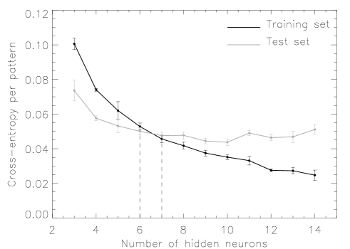
To find the optimal network architecture, we compare different solutions with between 3 and 14 hidden neurons on both the training set and the test set. The latter set comprises 10000 simulated microlensing lightcurves with noise and MACHO experimental sampling and 10000 non-microlensing events (variable stars and lightcurves drawn from MACHO LMC field 82 which has no candidate events). The cross-entropy error (see Bishop 1995, chap. 6) divided by the number of patterns for the training and test sets is shown in Figure 1 as a function of the number of hidden units. The cross-entropy error per pattern for the training set slowly declines with increasing number of neurons, but it begins to flatten at about 6 or 7 hidden neurons for the test set. Thus, we choose to combine networks with 6 and 7 hidden units to form a committee comprising in total 50 networks.

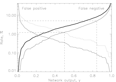
The committee is then applied to the test set to estimate the rate of false negatives (microlensing events misclassified as not microlensing) and false positives (non-microlensing events misclassified as microlensing). Note that the probabilities or rates of false negatives (or positives) are normalised to the total number of microlensing (or non-microlensing) lightcurves respectively. The results for the raw data are shown in Figure 2 in unbroken lines. The rate of false positives and false negatives are equal with a value of $0.8\%$ at a decision boundary of $y\approx 0.2$. However, most of the false negatives (genuine microlensing lightcurves with an output $y<0.2$) have less than 5 datapoints during the event with a signal-to-noise ratio $>5$. If we process only microlensing events with 5 or more such datapoints during the events, then the false negative rate is shown as the black dotted line in Figure 2. In fact, the MACHO collaboration applies a series of cuts to the raw data before analysis, which removes outliers prevalent in the data. To mimic this, we “clean” the raw data using the methods described by Belokurov et al (2003). If we process both raw and clean lightcurves, taking the maximum output of the two, then the false positive rate is increased as shown by the grey dotted line. A decision boundary corresponding to the point where the two dotted lines cross is $y=0.5$. The false positive and false negative rates in the test set are then both equal to $\sim 1\%$ for single passband data.

In practice, we can choose to be more or less conservative. In other words, we can reduce the incidence of false positive detections at the expense of increasing the rate of false negative detections, or vice versa. Where we choose this balance is controlled by the positioning of the decision boundary. As the MACHO data are taken in both blue and red passbands, the network is actually applied twice. For classification as microlensing, an event must pass in both passbands. Suppose the decision boundary corresponds to the false negative rate $P$ for single passband data. This means that – assuming that the distributions for each network are independent – the false positive rate for data in two passbands is $\sim P^{2}$ and the false negative rate is $\sim 2P$. We select $P$ by insisting that the number of false negatives in the entire MACHO dataset is $\mathrel{\hbox to0.0pt{\lower 3.0pt\hbox{$\sim$}\hss}\raise 2.0pt\hbox{$<$}}1$, Using the information that – as judged from the theoretical optical depth – the expected number of microlensing events in the entire MACHO dataset is $O(10)$, this yields $P=0.05$ which from the dotted curve in Figure 2 gives a decision boundary at $y=0.84$. This we adopt in the rest of the paper. It corresponds to a false positive rate of $0.3\%$

This choice of decision boundary gives rise to a negligible number of bona fide microlensing events that are classified as non-microlensing. Note that because non-microlensing is overwhelmingly more common than microlensing, there will be more false positives than false negatives.

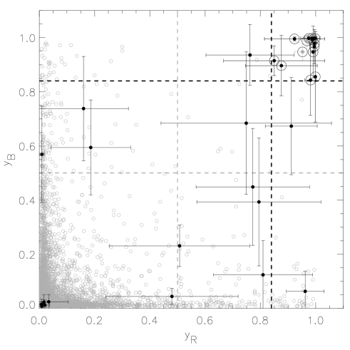
To illustrate this, Figure 3 shows the locations of $\approx 22000$ MACHO lightcurves. The data for the red and blue passbands are processed separately to give outputs $y_{R}$ and $y_{B}$. Again, the value of the output that is plotted is the maximum of the two outputs for the raw and the cleaned lightcurves. The error bars give the standard deviation of all the committee outputs. The decision boundary is shown in the bold broken line – convincing microlensing candidates have $y_{R,B}>0.84$. The 29 candidate lightcurves identified by Alcock et al. (2000) are denoted by filled black dots, while all other lightcurves are shown as open grey dots. The outputs for Alcock et al.’s 29 candidates are recorded in the first two columns of Table 2 and discussed in detail in Section 4. Twelve of these 29 lightcurves satisfy $y_{R,B}>0.84$, namely 1a, 1b, 5, 6, 10a, 11, 14, 21-25. There are additionally 2 false positives (with MACHO lightcurve numbers 17.2221.1377 and 17.2714.531) with $y_{R,B}>0.84$. The lightcurves of one of the false positives is illustrated in Figure 4. Both have a very low value for $x_{1}$ (the first input) and so they lie close to the noise/microlensing border in parameter space.

Figure 3 can be used to illustrate the effects of moving the decision boundary and therefore to assess the robustness of our results. Suppose the decision boundary were to be relocated to $y_{R}>0.5$ and $y_{B}>0.5$. We expect this to reduce the numbers of false negatives, at a cost of increasing the false positives. We now find that there are 9 false positives, 7 of which lie close to the noise/microlensing border. Additionally, there is one false positive that lies in an undersampled region of parameter space, and one that corresponds to a likely bumper. The gain is that a further 3 lightcurves are classified as microlensing (although these represent only 2 additional events).

3.2 A Network to remove the Supernovae

Figure 5: This shows the distributions of lightcurve shape features for microlensing (black) and supernovae (grey) in the training set. The timescale $x^{\prime}_{2}$ is shown in days, while the auto-correlation coefficient $x^{\prime}_{1}$ and the symmetry measure $x^{\prime}_{3}$ are dimensionless.

To distinguish microlensing from supernovae occuring in background galaxies is more problematic, as clearly pointed out in Alcock et al. (2000). This is the job of the next network in the cascade.

Gravitational microlensing of a point-source on a point-mass dark lens moving with a constant velocity produces a symmetric brightness change due to distortion of spacetime near the mass. A supernova lightcurve is generated by an exploding star and is characterised by a very quick rise followed by a steady decline. Based upon this knowledge, we might hope to use the symmetry of the lightcurve as a discriminant feature. However, microlensing lightcurves can appear much less symmetric when the observational campaign has irregular time sampling or when the beginning or end of the event is missed. On the other hand, supernova lightcurves can seem symmetric if only the top part of the lightcurve is sparsely sampled. This happens because distant supernovae are generally faint objects and only briefly enter the magnitude range of the survey.

Colour evolution during the event is another important discriminant. The colours change dramatically during a supernova explosion as a result of complicated radiation processes inside the ejecta. After a fairly constant pre-maximum epoch with $B-V\approx 0$, a supernova of type Ia typically starts turning red at the time of the maximum light, it reaches $B-V\approx 1$ in about 30 days and then drops back (see e.g., Phillips et al. 1999). This can be contrasted with the colour behaviour during gravitational microlensing. Gravity bends light irrespective of its frequency. Therefore, colour does not change during microlensing. However, the achromaticity of the lightcurve only holds good if the source star is resolved and the lens is dark. The presence of other stars within the centroid of light or lensing by a luminous object will result in a colour change during the event. At the baseline, the colour is defined by the combined flux from all the sources. The amplified star will contribute most of the colour around the peak. The colour of a microlensing event can become redder or bluer, depending on the population of the blend, but it usually changes symmetrically about the peak with substantial correlation between passbands (see e.g., Di Stefano & Esin 1995, Buchalter, Kamionkowski, & Rich 1996).

Again, we build a training set with patterns of features extracted from simulated microlensing and supernova lightcurves. Then, a committee of networks is trained and applied to the lightcurves of all transients found at the first stage of the data-mining. In the training set, simulated microlensing lightcurves have a slightly different timescale distribution as compared to Section 3.1. The value of the Einstein diameter crossing time is drawn from a Gaussian distribution with zero mean and standard deviation of 75 days. This is done to ensure that the set is dominated by fast transients, for which confusion with supernova lightcurves is most problematic. Blending is also added by changing the amplification to $(1-f_{B,R})+Af_{B,R}$ , where $A$ is the unblended amplification and the blending fractions in blue and red passbands $f_{B,R}$ are drawn from a Gaussian distribution with unit mean and standard deviation of 0.4.

We generate supernova lightcurves of type Ia only, as they are the most luminous and hence should be the dominant contaminant in any sample. For the templates, we use $R$ and $B$ passband data of supernova SN 1991T from Lira et al. (1998). This is an unusually bright supernova; however our algorithm chooses a random magnitude at maximum so only the shape of the lightcurve is important. The $R$ and $B$ colours from Lira et al. do not match MACHO passbands exactly since MACHO imaging was performed in non-standard red ($\lambda\lambda$ 5900-7800 Å) and blue ($\lambda\lambda$ 4370-5900 Å) filters. This should not be a serious concern since the training set data-cloud is smoothed by noise and irregular sampling. The simulated supernova lightcurve is a randomly chosen part of the top of the supernova template. We allow for extinction in the host galaxy by permitting the lightcurves in the blue and red passbands to have slightly different amplitudes. The total detected brightness change in magnitudes is $2.5\log[(u^{2}+2)/u\sqrt{u^{2}+4}]$, where $u$ is distributed uniformly between 0 and 1. In this way, the typical signal in the subset of supernovae events in the training set correlates with the typical signal in subset of microlensing events. All the lightcurves have Gaussian noise added and are sampled with actual MACHO sampling.

Figure 6: This shows distributions of colour features for microlensing (black) and supernovae (grey) in the training set. Mean colour change $x^{\prime}_{6}$ is in magnitudes, $x^{\prime}_{7}$ is mapped from (0,$\infty$) to (0.5,1) with the sigmoid function and $x^{\prime}_{8}$ is in logarithmic measure.

To describe the shape of the lightcurve, we extract the following features. First, $x^{\prime}_{1}$ is the maximum value of the autocorrelation coefficient. It can be regarded as a measure of the signal in the lightcurve. To make the feature extraction more robust, we take advantage of the fact that the lightcurve has already passed the first stage of classification. So we can assume that the epoch of the maximum light has been estimated by the first neural network. Thus, the second feature $x^{\prime}_{2}$ is the time between the peak and the instant when the amplification exceeds $1.34$. For microlensing events, an amplification of $1.34$ or greater means that projected position of the source lies within an Einstein radius of the lens, and so $x^{\prime}_{2}$ is exactly half the event duration. For supernova lightcurves, this feature is well-defined, but does not correspond to anything with a simple physical meaning. The third feature $x^{\prime}_{3}$ is the value of the cross-correlation of the lightcurve with the time-reversed lightcurve evaluated at lag $T$. Here, we use only the data-points within a timescale $x^{\prime}_{2}$ of the maximum in both the forward and backward directions (the Einstein diameter crossing time for microlensing). The lag $T$ is defined as the time difference between the instants of maximum brightness of the lightcurve and the time-reversed lightcurve. The parameters $(x^{\prime}_{1},x^{\prime}_{2},x^{\prime}_{3})$ are all extracted from the red lightcurve. The fourth $x^{\prime}_{4}$ and the fifth $x^{\prime}_{5}$ features are the autocorrelation and symmetry parameters extracted from the blue lightcurves.

Additionally, we feed the network with features characterizing the colour change during the event. Note, that when the signal to noise of the transient is low or when the colour change is minuscule, then the error propagation might result in the destruction of any colour signal. In other words, any signal in the colour is noisier than the corresponding signal in the red or blue passbands separately. Irregularity of the time sampling can further aggravate the problem, since not all the measurements are taken simultaneously in both colours. To account for this and to stabilize the colour, we extract all the following features from lightcurves binned with a time bin-size of 2 days. To estimate the total colour change during the event, we calculate the weighted average excursion from the colour baseline:

$$x^{\prime}_{6}=\left.\sum_{i=1}^{n}\frac{|(B-R)_{i}-(B-R)_{0}|}{\sigma^{2}_{B-R,i}}\right/\sum_{i=1}^{n}\frac{1}{\sigma^{2}_{B-R,i}}.$$ (3)

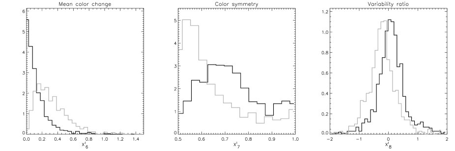
Here, the index $i$ runs through all measurements within the Einstein diameter crossing time and the baseline $(B-R)_{0}$ is the weighted average colour outside the Einstein crossing time. The next feature $x^{\prime}_{7}$ is the ratio of total weighted absolute colour change before and after the maximum light. This tests the symmetry of the colour signal. For microlensing, this ratio takes values around 1, while for supernova lightcurves it is close to zero. Therefore, we magnify the range between 0 and 1 by transforming the ratio with the sigmoid function. Finally, the last colour feature is the variability ratio as defined by Welch & Stetston (1993). It is the ratio of the total normalized magnitude residuals in the blue and red filters, namely

$$x^{\prime}_{8}=\left.\sum_{i=1}^{n}|\delta B|\right/\sum_{i=1}^{n}|\delta R|,$$ (4)

where

$$\delta B=\frac{B_{i}-\overline{B}}{\sigma_{B_{i}}},\qquad\delta R=\frac{R_{i}-\overline{R}}{\sigma_{R_{i}}},$$ (5)

Here the weighted means $\overline{B},\overline{R}$ are calculated over all epochs outside the Einstein crossing time. We take the logarithm of the variability ratio so as to compress the range. Supernovae lightcurves have, on average, smaller values of $x^{\prime}_{8}$ than microlensing lightcurves.

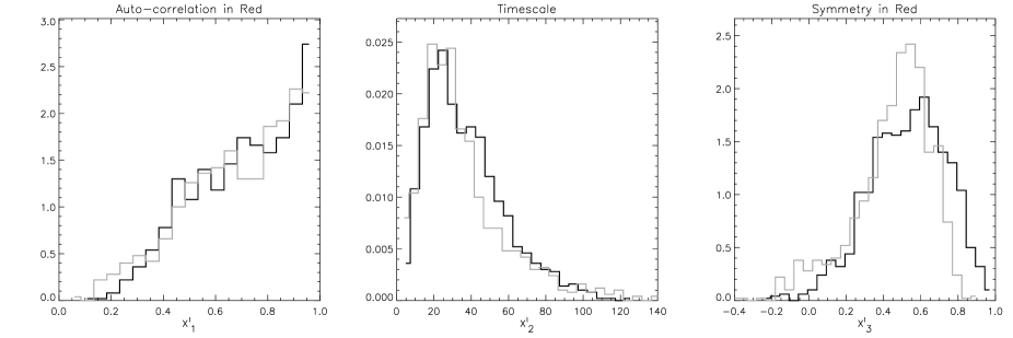
The distributions of lightcurve shape features are shown in Figure 5. It is clear from the first two panels that $x^{\prime}_{1}$ and $x^{\prime}_{2}$ serve as control features. The autocorrelation and timescale distributions of supernova and microlensing lightcurves do not differ much. This is reassuring since it indicates that we are probing similar signal regimes of the two different variability classes. The distribution of $x^{\prime}_{3}$ (the third panel of Figure 5) confirms our choice of this feature as a symmetry measure with microlensing dominating around values of $\mathrel{\hbox to0.0pt{\lower 3.0pt\hbox{$\sim$}\hss}\raise 2.0pt\hbox{$>$}}0.8$.

Figure 6 shows the distribution of colour related parameters. From the first panel, it follows that, as expected, the amplitude of the colour change is significantly lower for microlensing. Note, however, that there is a tail in the $x^{\prime}_{6}$ distribution that stretches as far as 1.5 magnitudes for both microlensing and supernovae. The colour signal looks very symmetric for microlensing with $x^{\prime}_{7}$ peaking at $\sim 0.7$. Let us recall that the original colour symmetry ratio was transformed with the sigmoid function, which means that 1 is mapped onto value $\simeq 0.73$. The distribution of $x^{\prime}_{7}$ for the supernova lightcurves peaks around 0.55, which corresponds to a value of 0.2 in the symmetry ratio. Finally, the variability ratio $x^{\prime}_{8}$ is presented in the third panel of this figure. The mean value of the logarithm of $x^{\prime}_{8}$ for microlensing is zero and the distribution itself is symmetric, while supernovae prefer smaller values of this feature, typically by factor of $10^{-0.2}\simeq 1.6$.

The total number of patterns in the training set is 2000, one half are extracted from microlensing lightcurves and the other half from the simulated lightcurves of supernovae. For networks with more than 5 neurons, the data misfit keeps decreasing monotonically. We therefore choose to use 10 networks with 5 hidden units to form the committee. The candidate microlensing events towards the LMC are then processed with the network and the outputs recorded in the third column of Table 2. The output $y^{\prime}$ can be interpreted as the probability that the lightcurve is not a supernova. The optimum decision boundary can be found by examining the false positive and negative rates as in Section 3.1; however, for the purposes of this paper, it suffices to interpret $y^{\prime}\ll 0.5$ as a strong supernova candidate, $y^{\prime}\gg 0.5$ as definitely not a supernova, and $y^{\prime}\approx 0.5$ as indeterminate.

Event	$y_{R}$	$y_{B}$	$y^{\prime}$
1a	0.88 $\pm$ 0.13	0.90 $\pm$ 0.11	0.97 $\pm$ 0.01
1b	0.99 $\pm$ 0.01	0.98 $\pm$ 0.03	0.95 $\pm$ 0.01
4	0.81 $\pm$ 0.18	0.12 $\pm$ 0.13	0.90 $\pm$ 0.02
5	0.99 $\pm$ 0.002	0.86 $\pm$ 0.17	0.74 $\pm$ 0.18
6	0.98 $\pm$ 0.03	0.99 $\pm$ 0.003	0.97 $\pm$ 0.02
7a	0.77 $\pm$ 0.21	0.45 $\pm$ 0.22	0.84 $\pm$ 0.10
7b∗	0.02 $\pm$ 0.02	0.02 $\pm$ 0.02	0.21 $\pm$ 0.05
8	0.51 $\pm$ 0.25	0.23 $\pm$ 0.08	0.86 $\pm$ 0.04
9∗,binary	0.76 $\pm$ 0.16	0.94 $\pm$ 0.11	0.67 $\pm$ 0.13
10aSN	0.85 $\pm$ 0.18	0.92 $\pm$ 0.05	0.82 $\pm$ 0.12
10bSN	0.16 $\pm$ 0.16	0.74 $\pm$ 0.19	0.88 $\pm$ 0.01
11∗,SN	0.98 $\pm$ 0.02	0.84 $\pm$ 0.13	0.05 $\pm$ 0.01
12aSN	0.96 $\pm$ 0.07	0.06 $\pm$ 0.07	0.01 $\pm$ 0.01
12bSN	0.75 $\pm$ 0.31	0.68 $\pm$ 0.26	0.42 $\pm$ 0.25
13	0.03 $\pm$ 0.07	0.03 $\pm$ 0.03	0.96 $\pm$ 0.04
14	0.92 $\pm$ 0.11	0.99 $\pm$ 0.007	1.00 $\pm$ 0.00
15	0.01 $\pm$ 0.01	0.01 $\pm$ 0.01	0.84 $\pm$ 0.03
16∗,SN	0.01 $\pm$ 0.01	0.57 $\pm$ 0.18	-
17∗,SN	0.01 $\pm$ 0.01	0.02 $\pm$ 0.02	0.04 $\pm$ 0.01
18	0.91 $\pm$ 0.09	0.68 $\pm$ 0.18	0.95 $\pm$ 0.03
19∗,SN	0.02 $\pm$ 0.02	0.01 $\pm$ 0.02	0.07 $\pm$ 0.06
20∗	0.8 $\pm$ 0.22	0.39 $\pm$ 0.24	0.23 $\pm$ 0.20
21	0.99 $\pm$ 0.03	0.99 $\pm$ 0.02	1.00 $\pm$ 0.00
22	0.99 $\pm$ 0.001	0.99 $\pm$ 0.002	0.98 $\pm$ 0.01
23	0.99 $\pm$ 0.01	0.99 $\pm$ 0.01	0.96 $\pm$ 0.01
24∗,SN	0.99 $\pm$ 0.005	0.97 $\pm$ 0.06	0.61 $\pm$ 0.26
25	0.99 $\pm$ 0.01	0.95 $\pm$ 0.1	0.98 $\pm$ 0.01
26∗,SN	0.19 $\pm$ 0.14	0.59 $\pm$ 0.18	0.87 $\pm$ 0.02
27∗	0.48 $\pm$ 0.24	0.04 $\pm$ 0.03	0.70 $\pm$ 0.01

Table 2: This shows the output of the committee of neural networks (the posterior probability of microlensing) on the set of candidates towards the LMC identified by Alcock et al. (2000). Stars mark events that did not pass MACHO’s selection criteria A. A superscript SN marks a supernova as judged by Alcock et al. (2000). The first two columns ($y_{R}$ and $y_{B}$) are the outputs of the network of Section 3.1 on the red and blue data, the third column ($y^{\prime}$) is the output of the network of Section 3.2.

4 New light on the MACHO candidates

First, let us recall that Alcock et al. (2000) used a series of conventional cuts to identify microlensing events. The set A selection criteria are “designed to accept high quality microlensing candidates”. The set B criteria are “designed to accept any light curves with a significant unique peak and a fairly flat baseline”. 19 lighcurves pass the set A criteria and 29 pass the looser set B. Sometimes the same source star has two lightcurve because, for example, it lies in an overlap region. Eight of the 29 lightcurves (1a, 1b, 7a, 7b, 10a, 10b, 12a and 12b) correspond to just four stars. Finally, Alcock et al. apply a supernova cut, insisting that a blended microlensing lightcurve is a better fit than a SN Ia template. This finally leaves 13 events in set A (events 1, 4-8, 13-15, 18, 21, 23 and 25) and 17 events in set B (everything in set A together with 9, 20, 22 and 27). Subsequently, event 22 was confirmed to be a Seyfert galaxy and so can be removed from set B (Sutherland, private communication).

4.1 Microlensing versus Variable Stars

Figure 7: This shows the colour evolution of events 5 and 11. Event 5 shows a colour shift that changes symmetrically about the peak in the flux of the event. This is characteristic of blended microlensing events. Event 11 is a supernova candidate, as evidenced by the stable colour in the pre-maximum epoch, the rapid reddening at maximum, followed by the colour becoming increasingly blue. The classical supernova colour curve as depicted in Lira et al. (1998) is shifted because of extinction in the host galaxy. The vertical axis is $B-R$ in magnitudes and the horizontal axis is time in JD-2448000. The dotted vertical line is the peak of the event, while the dashed vertical lines mark the time over which the amplification exceeds $1.34$.

Figure 8: This shows the lightcurves for 4 events which received low probability values $y$ in one or both filters. These are all included in set A of Alcock et al. (2000) of convincing microlensing candidates, but are not confirmed by our neural network analysis. The vertical axis is flux in ADU s^-1 and the horizontal axis is time in JD-2448000. Vertical lines mark the peak of the event.

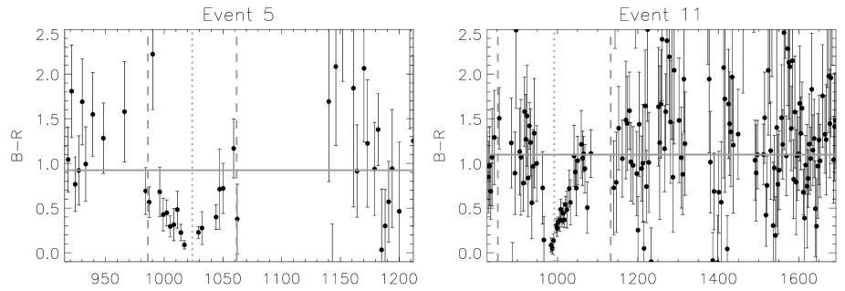
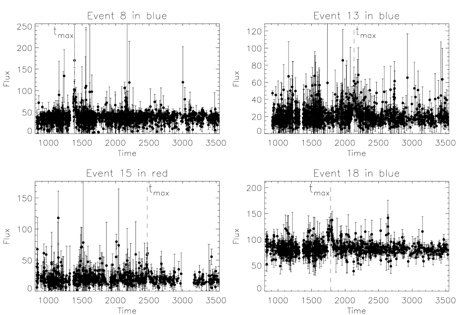
Table 2 shows the predictions of committees of neural networks for the LMC microlensing candidates selected by MACHO. First, let us concentrate on the output in the first two columns which is provided by the committee of neural networks to eliminate variable stars (see section 3.1). Let us recall that the output $y$ is the posterior probability of microlensing.

In total, 7 out of 13 candidates from MACHO set A receive $y>0.84$ in both red and blue filters: 1, 5, 6, 14, 21, 23, 25. These events can be regarded as secure microlensing identifications.

Six events from MACHO set A fail the test for microlensing. Event 18 is a marginal case, as it is identified in the red ($y_{R}=0.91$) but not in the blue ($y_{B}=0.68$). It is a low signal-to-noise event, with one of the smallest maximum amplifications $A_{\rm max}=1.54$. Events 4, 7, 8, 13 and 15 have $y<0.84$ in both bands. Some of these lightcurves are noisy with no stable baseline, such as events 13 and 15. Event 8 has an apparently asymmetric shape, partly because the beginning of the event is lacking due to a gap in the observational campaign. The lightcurves of some of the failed events are shown in Figure 8.

One of the lightcurves that was selected by MACHO as a result of applying only the loose selection criteria B gets an output $y_{R,B}>0.84$. This is event 22. The remaining three candidates – events 9, 20 and 27 – all fail our microlensing test of $y_{R,B}>0.84$.

The four supernova suspects as judged by MACHO (events 16, 17, 19, 26) fail the microlensing network committee. The other three candidates also suspected by MACHO of being supernova lightcurves, 10a, 11 and 24, are classified with probability $y_{R,B}>0.84$. They are, however, discarded after being tested with the second neural network committee.

4.2 Microlensing versus Supernovae

Convincing supernova candidates must have an output $y^{\prime}\ll 0.5$ from the second neural network committee. There are five events satisfying this, namely the 4 MACHO supernova suspects (11, 12a,b, 17, 19) plus candidate 20. The colour evolution of event 11 is illustrated in Figure 7. Although not identified by MACHO as a supernova candidate, event 20 has a typical supernova colour evolution. MACHO claims there are four more supernovae in the dataset, namely events 10a,b, 16, 24 and 26. Unfortunately, candidate 16 has no information in the red filter, but it is classified as non-microlensing in the blue colour by the first network. Event 24 has probability $y^{\prime}=0.6$, the error is large and – to be conservative – we conclude its origin is unknown.

Candidates 10a,b and 26 have outputs greater than 0.8. These two events have timescales of $\sim 40$ days. If they are indeed supernovae, it means that signal is present only for $\sim 20$ days after the maximum light. The colour reaches a maximum after $\sim 30$ days, but even after 20 days B-V can be as much as $0.5-1.0$ mag (see Figure 1 in Phillips et al. 1999). Neither event 10a,b nor 26 shows any significant colour change. Hence, we do not confirm the supernova classification of Alcock et al. (2000).

There is just one candidate that has a substantial colour signal identified as blended microlensing by the neural networks. This is event 5. The colours evolve symmetrically during the event, which becomes $\sim 1$ mag bluer. It has output $y^{\prime}=0.74$ and is illustrated in Figure 7.

4.3 Numbers of Events

In conclusion, then, the committees of neural networks reckons that there are 7 convincing microlensing candidates. These are the events 1, 5, 6, 14, 21, 23 and 25. All these events have an output that always lies above the decision boundary $y>0.84$. They also judged to be not supernovae ($y^{\prime}\gg 0.5$). Of the remaining events, 10a and 18 are possible, but not convincing, microlensing candidates.

Compared to Alcock et al.’s (2000) set A, we have discarded events 4, 7, 8, 13, 15 and 18 (which is a marginal case). Four of the events that we have excised from Alcock et al.’s sample A are shown in Figure 8. In each case, we show the data from the passband which yields the lowest network probability. None of the events in set B (events 9, 20 and 27) are identified as microlensing by the committee, while event 22 is known to be a Seyfert on other grounds

Alcock et al. reckoned there were 8 supernova suspects. We confirm 4 of these (events 11, 12, 17, 19) and we also found 1 new one (event 20). The remainder of Alcock et al’s supernova candidates are not thought to be either convincing supernova or microlensing candidates by the committees.

4.4 Optical Depth

How does this affect the optical depth results? In qualitative terms, the optical depth must be significantly lower than the value of $1.2^{+0.4}_{-0.3}\times 10^{-7}$ of Alcock et al. (2000) and more in accord with the results of the EROS collaboration (Laserre et al. 2000). This is because the number of convincing microlensing candidates has been reduced from 17 to 7 in our analysis. However, in quantitative terms, the optical depth is not so easy to compute without re-processing the entire MACHO dataset of $\sim 11.9$ million lightcurves. There may be lightcurves that the neural networks identify as microlensing, even though MACHO did not. This seems unlikely, as no new candidates emerged from the $\approx 22000$ MACHO lightcurves we have re-processed. However, it cannot yet be ruled out, and so we do not provide an estimate for the optical depth from our neural networks. Here, we merely note that the number of events has been roughly halved, and we speculate that a concomitant reduction in the optical depth might be expected.

5 Conclusions

This paper has demonstrated the power of machine learning techniques, such as neural networks, for the classification of events in massive variability datasets. Using the specific example of the microlensing surveys, committees of neural networks have been devised to discriminate against common forms of stellar variability and against supernovae. The output of the neural network is the posterior probability of microlensing, given the prior distribution in the training set. The error on the probability can be straightforwardly calculated.

The networks have been used to process some of the data ($\approx 22000$ lightcurves) taken towards the Large Magellanic Cloud by the MACHO collaboration (Alcock et al. 2000). The latter authors provide a set of 13 events whose identification as microlensing is believed to be secure and a further 4 events whose identification is possible. The neural networks confirm the microlensing nature of only 7 of these possible 17 events.

Without processing the entire dataset ($\sim 11.9$ million lightcurves), we cannot be sure that there are no events missed by Alcock et al. (2000) which would be classified as microlensing by the networks. It is reasonable to argue that this is unlikely, as the $\approx 22000$ MACHO lightcurves we have re-processed provide no new candidates. But, this remains a plausible speculation rather than an empirically derived fact. Hence, we can only speculate that, as the number of events has been roughly halved, so the optical depth will be similarly reduced.

For comparison, Alcock et al. (1997) estimate the optical depths of the thin disk, thick disk and spheroid to be $2.2\times 10^{-8}$, whilst the optical depth of the stellar content of the LMC to be $3.2\times 10^{-8}$ on average. In other words, from the known stellar populations in the outer Galaxy and the LMC, the optical depth must be at least $5.4\times 10^{-8}$. This may well be enough to provide the 7 events whose microlensing nature we confirm.

There is supporting evidence for the belief that the known stellar populations are providing the bulk of the lenses both from the exotic events and from the lensing signal towards the Small Magellanic Cloud (SMC). First, the exotic events yield additional information which can break some of the microlensing degeneracies and thus give indirect evidence on the location of the lens. There are two exotic events towards the LMC and two towards the SMC (Bennett et al. 1996; Palanque-Delabrouille 1998; Kerins & Evans 1999; Afonso et al. 2000; Alcock et al. 2001a; Evans 2002). In all cases, the exotic events favour an interpretation in which the lens lies in the Magellanic Clouds. Additionally, Alcock et al. (2001b) imaged one of the events towards the LMC and identified the lens as a nearby low mass disk star.

Second, as Afonso et al. (2003a) point out, the duration of the events towards the SMC is very different from the duration towards the LMC. The EROS collaboration constrain the optical depth towards the SMC to be $<10^{-7}$ at better than the 90 % confidence level, based on an admittedly small sample. Both these facts militate against the idea that a single population of objects in the Milky Way halo is causing the microlensing events. The mass function, internal kinematics and proper motions of the SMC and LMC are different, so that differences in the distributions of microlensing events are expected if the lenses lie predominantly in the Magellanic Clouds. Based on roughly spherical models of the dark halo, the optical depth towards the SMC is expected to be greater than that towards the LMC if the halo provides most of the lenses. Hence, the paucity of events towards the SMC is beginning to be highly problematic for halo interpretations of the events.

Appendix A Neural Network Estimators of the Microlensing Rate

It is interesting to develop methods of calculating the theoretical microlensing quantities directly from the outputs of neural networks.

Let us define $E(x)$ to be the ratio of the density of microlensing events in the training set to the true density, i.e.,

$$E(x)={P(x|C_{1})\over\hat{P}(x|C_{1})}$$ (6)

Here $\hat{P}(x|C_{1})$ is the conditional probability of microlensing (i.e., class 1) in the real world.

The output of the neural network is the posterior probability, and relies on the prior probabilities of different classes of variability in the training set. As follows from Table 1, the prior probability of microlensing in the training set is at least $10^{6}$ times larger than that in the real world. Indeed, the training set contains a large number of microlensing lightcurves to ensure a good variety of training examples. Therefore, the outputs of the trained neural network need to be adjusted with respect to the real-world priors. It has been shown (e.g., Saerens et al. 2002) that a simple iterative procedure can help to tackle the problem. For microlensing, it follows from Bayes’ theorem that:

$$\frac{P(C_{1}|x)P(x)}{P(C_{1})}=E(x)\frac{\hat{P}(C_{1}|x)\hat{P}(x)}{\hat{P}(C_{1})}$$ (7)

For variable stars, the same equation holds good without the correction for input space sampling, namely

$$\frac{P(C_{2}|x)P(x)}{P(C_{2})}=\frac{\hat{P}(C_{2}|x)\hat{P}(x)}{\hat{P}(C_{2})}$$ (8)

This assumes that the sampling never causes the misclassification of a variable star as a microlensing event. In our notation, quantities with a hat superscript refer to the real world, whereas unhatted quantities refer to the training set. Let us now recall that the activation $a$ of the output neuron can be interpreted as a logarithm of the ratio of posterior probabilities:

$$a\equiv\log\frac{P(C_{1}|x)}{P(C_{2}|x)}$$ (9)

This is simply the consequence of using the sigmoid function for activation. Applying formulae (7) and (8) to each of the two classes and taking the ratio of probabilities, we easily obtain:

$$\hat{a}=a(x)-\log\frac{E(x)P(C_{1})}{\hat{P}(C_{1})}+\log\frac{P(C_{2})}{\hat{P}(C_{2})}$$ (10)

Typically, $P(C_{1})/{\hat{P}}(C_{1})\sim 10^{7}$. If the activation was originally $\mathrel{\hbox to0.0pt{\lower 3.0pt\hbox{$\sim$}\hss}\raise 2.0pt\hbox{$<$}}7$, then this transformation maps it to below the decision boundary. Only if the output is originally $>0.999$ does the event remain above the decision boundary.

Thus, having initialized $P(C_{k})$ by the frequencies of the classes in the training set, we perform the following iterative steps. Firstly, the formula

$${\hat{P}}(C_{1})\approx\frac{1}{N}\sum_{i}y_{i}$$ (11)

is used to estimate the true probability of microlensing. Here, $i$ runs through all $N$ patterns in the data set. Then, for each pattern in the data set activation $a_{i}$ is adjusted using formula (10) and the output $y_{i}$ is re-calculated. The process is repeated until convergence. At the beginning of the iteration, $P(C_{1})/{\hat{P}}(C_{1})$ is $0(10^{7})$ so that the sampling factor $E(x)$ does not play an important role. However, after a few iterations, it becomes important. $E(x)$ is really a higher dimensional analogue of the temporal efficiency $\epsilon$. It can be calculated by generating events with uniform priors. In every cell of input space, we calculate the ratio of accepted events to generated events.

The output of this procedure is the true probability of microlensing in the experiment monitoring $N_{\star}$ stars and lasting for a duration $T$. From this, the microlensing rate is

$$\Gamma={N_{\star}{\hat{P}}(C_{1})\over T}$$ (12)

The advantage of this algorithm is that the rate can be computed directly from the dataset, without the intervening steps of candidate selection and efficiency estimation.

References

- [Afonso et al.(2000)] Afonso C. et al. 2000, ApJ, 532, 340
- [Afonso et al.(2003)] Afonso C. et al. 2003a, AA, 400, 951
- [Afonso et al.(2003)] Afonso C. et al. 2003b, AA, 404, 145
- [Alcock et al.(1997)] Alcock C. et al. 1997, ApJ, 479, 119
- [Alcock et al.(2000)] Alcock C. et al. 2000, ApJ, 542, 281
- [Alcock et al.(2001a)] Alcock C. et al. 2001a, ApJ, 552, 259
- [Alcock et al.(2001b)] Alcock C. et al. 2001a, Nature, 414, 617
- [Antonello & Morelli 1996] Antonello E., Morelli P.L. 1996, AA, 314, 541
- [An etal.(2004)] An J., et al. 2004, ApJ, 601, 845
- [Belokurov, Evans, & Du(2003)] Belokurov V., Evans N.W., Le Du Y. 2003, MNRAS, 341, 1373
- [Bennett et al. 1996] Bennett D.P. et al. 1996, Nucl. Physics, 51B, 131
- [Bishop ] Bishop C., 1995, Neural Networks for Pattern recognition, Oxford University Press, Oxford
- [Buchalter, Kamionkowski, & Rich(1996)] Buchalter A., Kamionkowski M., Rich R.M. 1996, ApJ, 469, 676
- [Di Stefano & Esin(1995)] Di Stefano R., Esin A.A. 1995, ApJ, 448, L1
- [Dominik(1998)] Dominik M. 1998, AA, 329, 361
- [Evans 2002] Evans N.W., 2002, In “IDM:2002 Fourth International Conference on the Identification of Dark Matter”, eds N. Spooner, V. Kudryavtsev, p. 144, World Scientific, Singapore, (astro-ph/0211302)
- [Kerins & Evans 1999] Kerins E.J., Evans N.W. 1999, ApJ, 517, 734
- [Lasserre et al.(2000)] Lasserre T. et al. 2000, AA, 355, L39
- [Lira et al. 1998] Lira P. et al. 1998, AJ, 115, 234
- [Mao et al.(2002)] Mao S. et al. 2002, MNRAS, 329, 349
- [Mao & Paczynski(1991)] Mao S., Paczynski B. 1991, ApJ, 374, L37
- [MacKay (1992a)] MacKay D.J.C. 1992a, Neural Computation, 4, 448
- [MacKay (1992b)] MacKay D.J.C. 1992b, Neural Computation, 4, 720
- [Nabney (2002)] Nabney I.T. 2002, Netlab: Algorithms for Pattern Recognition, Springer Verlag, New York
- [Paczynski(1986)] Paczynski B. 1986, ApJ, 304, 1
- [Palanque-Delabrouille 1998] Palanque-Delabrouille N. et al. 1998, AA, 332, 1
- [Phillips et al.(1999)] Phillips M.M., Lira P., Suntzeff N.B., Schommer R.A., Hamuy M., Maza, J. 1999, AJ, 118, 1766
- [Press et al. 1992] Press W.H., Teukolsky S., Vetterling W.T., Flannery B. 1992. Numerical Recipes, Cambridge University Press, Cambridge, 2nd ed. chap. 10.
- [Saerens et al 2002] Saerens M., Latinne P., Decaestecker C. 2002, Neural Computation, 14, 21
- [Welch & Stetson(1993)] Welch D.L., Stetson P.B. 1993, AJ, 105, 1813