The angular power spectrum of NVSS radio galaxies

Abstract

We measure the angular power spectrum $C_{\ell}$ of radio galaxies in the NRAO VLA Sky Survey (NVSS) using two independent methods: direct spherical harmonic analysis and maximum likelihood estimation. The results are consistent and can be understood using models for the spatial matter power spectrum and for the redshift distribution of radio galaxies at mJy flux-density levels. A good fit to the angular power spectrum can only be achieved if radio galaxies possess high bias with respect to mass fluctuations; by marginalizing over the other parameters of the model we derive a $68\%$ confidence interval $1.53<b_{0}\times\sigma_{8}<1.87$, where $b_{0}$ is the linear bias factor for radio galaxies and $\sigma_{8}$ describes the normalization of the matter power spectrum. Our models indicate that the majority of the signal in the NVSS $C_{\ell}$ spectrum is generated at low redshifts $z\la 0.1$. Individual redshifts for the NVSS sources are thus required to alleviate projection effects and probe directly the matter power spectrum on large scales.

1 Introduction

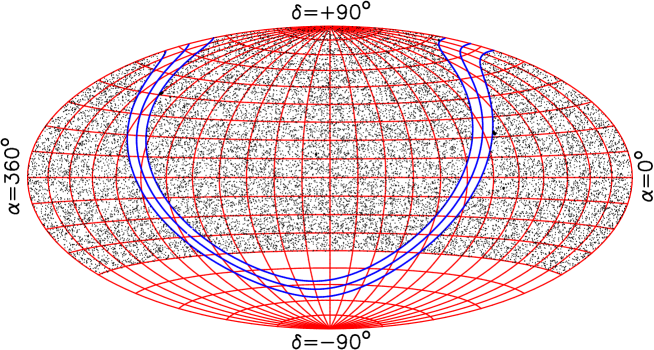
Figure 1: NVSS sources with $S_{\rm 1.4\,GHz}>200$ mJy in an equal-area projection. The Galactic plane and Galactic latitudes $\pm 5^{\circ}$ are also plotted; sources within this region are masked from our large-scale structure analysis as many are Galactic in origin.

Active Galactic Nuclei (AGN) mapped in radio waves are an interesting probe of large-scale structure. They can be routinely detected out to very large redshift ($z\sim 4$) over wide areas of the sky and hence delineate the largest structures and their evolution over cosmic epoch. Radio emission is insensitive to dust obscuration and radio AGN are effective tracers of mass: they are uniformly hosted by massive elliptical galaxies and have been shown to trace both clusters (Hill & Lilly 1991) and superclusters (Brand et al. 2003).

The current generation of wide-area radio surveys such as Faint Images of the Radio Sky at Twenty centimetres (FIRST; Becker, White & Helfand 1995) and the NRAO VLA Sky Survey (NVSS; Condon et al. 1998) contain radio galaxies in very large numbers ($\sim 10^{6}$) and have allowed accurate measurements of the imprint of radio galaxy angular clustering. These patterns are considerably harder to detect in radio waves than in optical light due to the huge redshift range that is probed. Whilst this provides access to clustering on the largest scales, it also washes out much of the angular clustering signal through the superposition of unrelated redshift slices. The angular correlation function was measured for FIRST by Cress et al. (1996) and Magliocchetti et al. (1998) and for NVSS by Blake & Wall (2002a) and Overzier et al. (2003).

The NVSS radio survey, covering $\sim 80$ per cent of the sky, permits the measurement of fluctuations over very large angles. Blake & Wall (2002b) detected the imprint of the cosmological velocity dipole in the NVSS surface density, in a direction consistent with the Cosmic Microwave Background (CMB) dipole. In this study we measure the angular power spectrum, $C_{\ell}$, of the radio galaxy distribution (Baleisis et al. 1998). This statistic represents the source surface-density field as a sum of sinusoidal angular density fluctuations of different wavelengths, using the spherical harmonic functions. The angular power spectrum is sensitive to large-angle fluctuations and hence complements the measurement of the angular correlation function, $w(\theta)$, at small angles.

Measurement of the $C_{\ell}$ spectrum has some advantages in comparison with $w(\theta)$. Firstly, the error matrix describing correlations between multipoles $\ell$ has a very simple structure, becoming diagonal for a complete sky. This is not the case for the separation bins in a measurement of $w(\theta)$: even for a full sky, an individual galaxy appears in many separation bins, automatically inducing correlations between those bins. Secondly, there is a natural relation between the angular power spectrum and the spatial power spectrum of density fluctuations, $P(k)$. This latter quantity provides a very convenient means of describing structure in the Universe for a number of reasons. Firstly its primordial form is produced by models of inflation, which prescribe the initial pattern of density fluctuations $\delta\rho/\rho$. Furthermore, in linear theory for the growth of perturbations, fluctuations described by different wavenumbers $k$ evolve independently, enabling the model power spectrum to be easily scaled with redshift. The physics of linear perturbations are hence more naturally described in Fourier space.

In contrast, the angular correlation function is more easily related to the spatial correlation function $\xi(r)$, the Fourier transform of $P(k)$. Correlation functions more naturally serve to describe the real-space profile of collapsing structures evolving out of the linear regime. We emphasize that although the two functions $C_{\ell}$ and $w(\theta)$ are theoretically equivalent – linked by a Legendre transform – this is not true in an observational sense. For example, $w(\theta)$ can only be successfully measured for angles up to a few degrees, but $C_{\ell}$ depends on $w(\theta)$ at all angles.

We derive the angular power spectrum using two independent methods. Firstly we apply a direct spherical harmonic estimator following Peebles (1973). Secondly, we use maximum likelihood estimation, commonly employed for deriving the angular power spectra of the CMB temperature and polarization maps. These two methods are described in Section 3. We find that these two approaches yield very similar results (Section 4), which is unsurprising given the wide sky coverage of the NVSS. In Section 5 we interpret the NVSS angular power spectrum in terms of the underlying spatial power spectrum of mass fluctuations and the radial distribution of radio sources. Finally in Section 6 we employ these models to derive the linear bias factor of NVSS radio galaxies by marginalizing over the other model parameters.

2 The NVSS radio survey

The 1.4 GHz NRAO VLA Sky Survey (NVSS; Condon et al. 1998) was performed at the Very Large Array over the period 1993 to 1996 and covers the sky north of declination $-40^{\circ}$. The source catalogue contains $\approx 1.8\times 10^{6}$ entries and is 99 per cent complete at integrated flux density $S_{\rm 1.4\,GHz}=3.5$ mJy. The full width at half-maximum of the synthesized beam is 45 arcsec; the majority of radio sources are thus unresolved. The relatively broad NVSS beam yields excellent surface brightness sensitivity and photometric completeness.

Before analyzing the survey for large-scale structure we imposed various angular masks. Firstly we excluded catalogue entries within $5^{\circ}$ of the Galactic plane, many of which are Galactic in origin (mostly supernova remnants and HII regions). The contribution of foreground Galactic sources at latitudes $|b|>5^{\circ}$ is negligible. We also placed 22 masks around bright local extended radio galaxies contributing large numbers of catalogue entries, as described in Blake & Wall (2002a). Figure 1 plots the remaining sources with $S_{\rm 1.4\,GHz}>200$ mJy. The remaining NVSS geometry corresponds to 75 per cent of the celestial sphere.

Blake & Wall (2002a) demonstrated that the NVSS suffers from systematic gradients in surface density at flux-density levels at which it is complete. These gradients – corresponding to a $\sim 5$ per cent variation in surface density at a threshold of 3 mJy – are entirely unimportant for the vast majority of applications of this catalogue. However, they have a significant influence on the faint imprint of large-scale structure. If left uncorrected a distortion of the measured angular power spectrum would result, because the harmonic coefficients would need to reproduce the systematic gradients as well as the fluctuations due to clustering.

Blake & Wall (2002a) found that these surface gradients are only significant at fluxes $S_{\rm 1.4\,GHz}<10$ mJy. At brighter fluxes the survey is uniform to better than 1 per cent – sufficient to allow the detection of the anticipated cosmological velocity dipole (Blake & Wall 2002b). Hence we simply restricted our $C_{\ell}$ analysis to fluxes $S_{\rm 1.4\,GHz}>10$ mJy. The NVSS source surface density at this threshold is $\sigma_{0}=16.9$ deg^-2.

We note that the broadness of the radio luminosity function ensures that the projected clustering properties of radio galaxies are not a strong function of flux density in the range 3 mJy $<S_{\rm 1.4\,GHz}<$ 50 mJy, as verified by the correlation function analyses of Blake & Wall (2002a) and Overzier et al. (2003). In this flux-density range, the redshift distribution of the radio galaxies does not change significantly.

3 Estimating the angular power spectrum: methods

3.1 Definition of the angular power spectrum

A distribution of galaxies on the sky can be generated in two statistical steps. Firstly, a density field $\sigma(\theta,\phi)$ is created; this may be described in terms of its spherical harmonic coefficients $a_{\ell m}$:

$$\sigma(\theta,\phi)=\sum_{\ell=0}^{\infty}\sum_{m=-\ell}^{+\ell}\,a_{\ell m}\,Y_{\ell m}(\theta,\phi)$$ (1)

where $Y_{\ell m}$ are the usual spherical harmonic functions. Secondly, galaxy positions are generated in a Poisson process as a (possibly biased) realization of this density field.

The angular power spectrum $C_{\ell}$ prescribes the spherical harmonic coefficients in the first step of this model. It is defined over many realizations of the density field by

$$<|a_{\ell m}|^{2}>=C_{\ell}$$ (2)

The assumption of isotropy ensures that $<|a_{\ell m}|^{2}>$ is a function of only $\ell$, not $m$.

The angular power spectrum $C_{\ell}$ is theoretically equivalent to the angular correlation function $w(\theta)$ as a description of the galaxy distribution. The two quantities are connected by the well-known relation

$$C_{\ell}=2\pi\,\sigma_{0}^{2}\int_{-1}^{+1}\,w(\theta)\,P_{\ell}(\cos{\theta})\,d(\cos{\theta})$$ (3)

where $\sigma_{0}$ is the source surface density and $P_{\ell}$ is the Legendre polynomial. However, the angular scales on which the signal-to-noise is highest are very different for each statistic. $w(\theta)$ can only be measured accurately at small angles up to a few degrees (Blake & Wall 2002a), beyond which Poisson noise dominates. By contrast, $C_{\ell}$ for galaxies has highest signal-to-noise at small $\ell$, corresponding to large angular scales $\theta\sim 180^{\circ}/\ell$. Hence the two statistics are complementary, the $C_{\ell}$ spectrum probing fluctuations on the largest angular scales.

3.2 Spherical harmonic estimation of $C_{\ell}$

Peebles (1973) presented the formalism of spherical harmonic analysis of a galaxy distribution over an incomplete sky (for refinements see e.g. Wright et al. 1994; Wandelt, Hivon & Gorski 2000). For a partial sky, a spherical harmonic analysis is hindered by the fact that the spherical harmonics are not an orthonormal basis, which causes the measured coefficients $a_{\ell m}$ to be statistically correlated, entangling different multipoles of the underlying $C_{\ell}$ spectrum. However, for the case of a survey covering $\sim 80\%$ of the sky, the repercussions (discussed below) are fairly negligible, implying shifts and correlations in the derived power spectrum that are far smaller than the error bars. We employed the original method of Peebles (1973) with only one small correction for sample variance. In Section 3.4 we compare spherical harmonic analysis with the technique of maximum likelihood estimation and find that the two methods yield results in good agreement.

The spherical harmonic coefficients of the density field may be estimated by summing over the $N$ galaxy positions $(\theta_{i},\phi_{i})$:

$$A_{\ell m}=\sum_{i=1}^{N}\,Y_{\ell m}^{*}(\theta_{i},\phi_{i})$$ (4)

For an incomplete sky, these values need to be corrected for the unsurveyed regions, so that an estimate of $C_{\ell}$ is

$$C_{\ell m}^{\rm obs}=\frac{|A_{\ell m}-\sigma_{0}\,I_{\ell m}|^{2}}{J_{\ell m}}-\sigma_{0}$$ (5)

(Peebles 1973 equation 50) where $\sigma_{0}=N/\Delta\Omega$ and

$$I_{\ell m}=\int_{\Delta\Omega}\,Y_{\ell m}^{*}\,d\Omega$$ (6)

$$J_{\ell m}=\int_{\Delta\Omega}\,|Y_{\ell m}|^{2}\,d\Omega$$ (7)

where the integrals are over the survey area $\Delta\Omega$, and are determined in our analysis by numerical integration. The final term in equation 5 corrects for the finite number of discrete sources: for a full sky ($I_{\ell m}=0,J_{\ell m}=1$) we expect $<|A_{\ell m}|^{2}>=\sigma_{0}$ in the absence of clustering, i.e. this is the power spectrum of the shot noise. Note that $\sigma_{0}$ is the apparent source density $N/\Delta\Omega$, not the average over an imagined ensemble of catalogues.

We determined the angular power spectrum for the $\ell$th multipole, $C_{\ell}^{\rm obs}$, by averaging equation 5 over $m$. Because the density field is real rather than complex, $C_{\ell m}^{\rm obs}=C_{\ell,-m}^{\rm obs}$, resulting in $\ell+1$ independent measurements of $C_{\ell}$:

$$C_{\ell}^{\rm obs}=\frac{\sum_{m=0}^{\ell}\,C_{\ell m}^{\rm obs}}{\ell+1}$$ (8)

There is no need for us to use the modified weighting formula of Peebles (1973 equation 53). In our case, $J_{\ell m}$ does not vary significantly with $m$. We verified that the modified weighting formula produced indistinguishable results.

One consequence of the partial sky is to “mix” the harmonic coefficients such that the measured angular power spectrum at $\ell$ depends on a range of $C_{\ell^{\prime}}$ around $\ell^{\prime}=\ell$:

$$<C_{\ell}^{\rm obs}>=\sum_{\ell^{\prime}}\,C_{\ell^{\prime}}\,R_{\ell\ell^{\prime}}$$ (9)

The angled brackets refer to an imagined averaging over many realizations of density fields generated by $C_{\ell}$, in accordance with equation 2. Peebles showed that $\sum_{\ell^{\prime}}R_{\ell\ell^{\prime}}=1$; i.e. mixing does not spuriously enhance the measured power (this is accomplished by the factor $J_{\ell m}$ in equation 5).

For a complete sky, $R_{\ell\ell^{\prime}}=\delta_{\ell\ell^{\prime}}$, where $\delta_{mn}=1$ ($m=n$) or 0 ($m\neq n$). For a partial sky, the matrix $R_{\ell\ell^{\prime}}$ can be computed from the geometry of the surveyed region (Hauser & Peebles 1973). Figure 2 illustrates the result for the NVSS for $\ell=10$ (computed using Hauser & Peebles 1973 equation 12). The NVSS covers a sufficiently large fraction of the sky (75 per cent) that mixing only occurs at the $\sim 15$ per cent level and can be neglected because the underlying $C_{\ell}$ spectrum is smooth:

$$<C_{\ell}^{\rm obs}>\approx C_{\ell}$$

We checked the NVSS $R_{\ell\ell^{\prime}}$ matrix for other multipoles $\ell$ and found very similar results. This argument ensures that the measured multipoles are statistically independent to a good approximation.

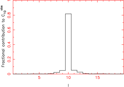
Figure 2: The range of $\ell$ probed by a measurement of $C_{\ell}^{\rm obs}$ at $\ell=10$. The incomplete sky means that $C_{10}^{\rm obs}$ is not just sensitive to $C_{10}$, but also to the surrounding $C_{\ell}$’s. However, the large fraction of sky covered means that this mixing is small.

The statistical error on the estimator of equation 5 is

$$\sigma(C_{\ell m}^{\rm obs})\approx(\sigma_{0}+C_{\ell})\sqrt{1+\delta_{m0}}$$ (10)

(Peebles 1973 equation 81). There are two components of the error:

• “Shot noise” ($\sigma_{0}$) because the number of discrete objects is finite and therefore does not perfectly describe the underlying density field.

• “Cosmic variance” ($C_{\ell}$) because even with perfect sampling of the density field, there are only a finite number of harmonics associated with the $\ell$th multipole.

The error for the $m=0$ case in equation 10 is greater because $A_{\ell 0}$ is purely real, rather than complex. In the latter case, we are averaging over the real and imaginary parts of $A_{\ell m}$, two independent estimates of $C_{\ell}$, which reduces the overall statistical error by a factor $\sqrt{2}$. For a partial sky equation 10 is an approximation, because the variance of multipoles of given $\ell$ depends on the underlying power spectrum at $\ell^{\prime}\neq\ell$. As discussed above, this effect is negligible for the NVSS.

The averaging over $m$ (equation 8) decreases the error in the observation. Combining the errors of equation 10, assuming estimates at different $m$ are statistically independent, the resulting error in $C_{\ell}^{\rm obs}$ is

$$\sigma(C_{\ell}^{\rm obs})\approx(\sigma_{0}+C_{\ell})\frac{\sqrt{\ell+2}}{\ell+1}$$ (11)

We used Monte Carlo simulations to verify that equation 11 produced results within 5 per cent of the true error for all relevant multipoles.

Our only addition to the formalism of Peebles (1973) was to increase the total variance on the estimate of $C_{\ell}$ by a factor $1/f_{\rm sky}$, where $f_{\rm sky}=\Delta\Omega/4\pi$ is the fraction of sky covered (i.e. multiply equation 11 by $1/\sqrt{f_{\rm sky}}$). This correction factor was motivated by Scott, Srednicki and White (1994) as a fundamental property of sample variance for a partial sky, and is part of the standard CMB formalism (e.g. Bond, Efstathiou & Tegmark 1997). For the NVSS geometry, $f_{\rm sky}=0.75$, thus this correction corresponds to a $\sim 10$ per cent increase in the error.

3.3 Correction for multiple-component sources

Radio sources have complex morphologies and large linear sizes (up to and exceeding 1 Mpc). A radio-source catalogue such as the NVSS will contain entries which are different components of the same galaxy (for example, the two radio lobes of a “classical double” radio galaxy). The broad angular resolution of the NVSS beam leaves over 90 per cent of radio sources unresolved; however, the remaining multiple-component sources have a small but measurable effect on the angular power spectrum.

It is relatively simple to model the effect of multiple-component sources on the estimator for $C_{\ell}$ described in Section 3.2. The relevant angular scales ($\ell<100$) are much bigger than any component separation, and equation 4 can be replaced by

$$A_{\ell m}=\sum_{i=1}^{N_{\rm gal}}c_{i}Y_{\ell m}^{*}(i)$$

where $N_{\rm gal}$ is the total number of galaxies and $c_{i}$ is the number of components of the $i$th galaxy. Thus the quantity

$$<A_{\ell m}>=N_{\rm gal}\,\overline{c}<Y_{\ell m}>=N<Y_{\ell m}>$$

is unchanged by the presence of multiple components ($\overline{c}$ denotes the average number of components per galaxy, and $N=\overline{c}\times N_{\rm gal}$ is the total number of catalogue entries, as in equation 4). But $C_{\ell m}^{\rm obs}$ in equation 5 depends on

$$<|A_{\ell m}|^{2}> = N_{\rm gal}\,\overline{c^{2}}<|Y_{\ell m}|^{2}>+N_{\rm gal}^{2}\,\overline{c}^{2}<Y_{\ell m}><Y_{\ell m}^{*}>$$

$$= \frac{\overline{c^{2}}}{\overline{c}}\,N<|Y_{\ell m}|^{2}>\,+\,N^{2}<Y_{\ell m}><Y_{\ell m}^{*}>$$

Multiple-component sources only affect the first term in this expression, producing an offset in the $C_{\ell}$ spectrum

$$\Delta C_{\ell}=\frac{\Delta(<|A_{\ell m}|^{2}>)}{J_{\ell m}}=\left(\frac{\overline{c^{2}}}{\overline{c}}-1\right)\frac{N<|Y_{\ell m}|^{2}>}{J_{\ell m}}$$

But $J_{\ell m}=<|Y_{\ell m}|^{2}>\Delta\Omega$ from equation 7, and this expression simplifies to an offset independent of $\ell$:

$$\Delta C_{\ell}=\left(\frac{\overline{c^{2}}}{\overline{c}}-1\right)\sigma_{0}$$

Most multiple-component sources in the NVSS catalogue are double radio sources. Let a fraction $e\ll 1$ of the radio galaxies be doubles. Then $\overline{c}=1+e$ and $\overline{c^{2}}=1+3e$, thus the constant offset may be written

$$\Delta C_{\ell}\approx 2\,e\,\sigma_{0}$$ (12)

We can deduce $e=0.07\pm 0.005$ from the form of the NVSS angular correlation function $w(\theta)$ at small angles $\theta<0.1^{\circ}$, where double sources dominate the close pairs (see Blake & Wall 2002a and also Section 4.2). This correction was applied to the measured NVSS $C_{\ell}$ spectrum and successfully removed the small systematic offset in $C_{\ell}$ at high $\ell$.

3.4 Maximum likelihood estimation of $C_{\ell}$

A sophisticated suite of analytical tools has been developed by the CMB community for deriving the angular power spectra of the observed CMB temperature and polarization maps. These methods can also be exploited to analyze galaxy data (see for example Efstathiou & Moody 2001, Huterer, Knox & Nichol 2001 and Tegmark et al. 2002). In this approach the power spectrum is determined using an iterative maximum likelihood analysis, in contrast to the direct estimator discussed in Section 3.2. The likelihood is a fundamental statistical quantity, and this analysis method permits straightforward control of such issues as edge effects, noise correlations and systematic errors.

The starting point for maximum likelihood estimation (MLE) is Bayes’ theorem

$$P(\alpha|DI)\propto P(\alpha|I)\,P(D|\alpha I)$$

where $\alpha$ are the parameters one is trying determine, $D$ is the data and $I$ is the additional information describing the problem. The quantity $P(\alpha|I)$ is the likelihood, i.e. the probability of the data given a specific set of parameters, while the left-hand side is the posterior, i.e. the probability of the parameters given the data.

We will assume that the sky is a realization of a stationary Gaussian process, with an angular power spectrum $C_{\ell}$. We assume no cosmological information about the distribution of the $C_{\ell}$. The rendition of the sky will be a pixelized map, created by binning the galaxy data in equal-area cells such that the count in the $i$th cell is $n_{i}$, effectively constructing a “temperature map” of galaxy surface density. We performed this task using the HEALPIX software package (Gorksi, Hivon & Wandelt 1999; http://www.eso.org/science/healpix). We chose the HEALPIX pixelization scheme $n_{\rm side}=32$, which corresponds to 12,288 pixels over a full sky. The angular power spectrum may be safely extracted to multipole $\ell_{\rm max}\approx 2\times n_{\rm side}$. We then defined a data vector:

$$x_{i}=\frac{n_{i}}{\overline{n}}-1$$ (13)

where $\overline{n}$ is the mean count per pixel. Figure 3 demonstrates that the data vector $x_{i}$ for the NVSS sample is well-approximated by a Gaussian distribution, as assumed in a maximum likelihood analysis.

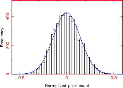
Figure 3: Maximum likelihood estimation assumes a Gaussian distribution for the pixelized data. This histogram shows the distribution of values of $x_{i}$ (see equation 13) for the NVSS 10 mJy sample, pixelized using HEALPIX parameter $n_{\rm side}=32$. The overplotted Gaussian curve demonstrates that Gaussianity is a good approximation for this sample.

The covariance matrix $C^{T}_{ij}$ due to primordial fluctuations is given by

$$\langle x_{i}x_{j}\rangle\,C^{T}_{ij}=\sum_{\ell}\frac{(2\ell+1)}{4\pi}\,C_{\ell}\,P_{\ell}(\cos\theta_{ij})$$

where $P_{\ell}$ is the Legendre polynomial and $\theta_{ij}$ is the angle between pixel pair $(i,j)$. In order to apply a likelihood analysis we must also specify a noise covariance matrix $C^{N}_{ij}$. We modelled the noise as a Gaussian random process with variance $1/\overline{n}$, uncorrelated between pixels, such that $C^{N}_{ij}=(1/\overline{n})\,\delta_{ij}$.

The likelihood of the map, with a particular power spectrum $C_{\ell}$, is given by

$$\ln P(C_{\ell}|{\bf x})\propto-\frac{1}{2}({\bf x}^{T}(C^{T}+C^{N})^{-1}{\bf x})+Tr[\ln(C^{T}+C^{N})]$$

The goal of MLE is to maximize this function, and the fastest general method is to use Newton-Raphson iteration to find the zeroes of the derivatives in $\ln P(C_{\ell}|{\bf x})$ with respect to $C_{\ell}$. We used the MADCAP package (Borrill 1999; http://www.nersc.gov/$\sim$borrill/cmb/madcap) to derive the maximum likelihood banded angular power spectrum from the pixelized galaxy map and noise matrix. MADCAP is a parallel implementation of the Bond, Jaffe & Knox (1998) maximum-likelihood algorithms for the analysis of CMB datasets. We ran the analysis software on the supercomputer Seaborg, administered by the National Energy Research Scientific Computing Centre (NERSC) at Lawrence Berkeley National Laboratory, California. We again applied equation 12 to the MADCAP results to correct the measured power spectrum for the influence of multiple-component sources.

Boughn & Crittenden (2002) also performed a HEALPIX analysis of the NVSS as part of a cross-correlation analysis with the CMB searching for evidence of the Integrated Sachs-Wolfe effect. From the pixelized map they derived an angular correlation function for the NVSS, which they used to constrain theoretical models. We compare their results with ours in Section 6.

3.5 Testing the methods

We tested the two methods, direct spherical harmonic and maximum likelihood estimation, by generating a dipole distribution of $N\approx 10^{5}$ sources over the NVSS geometry, where the model dipole possessed the same amplitude and direction as that detected in the NVSS (see Blake & Wall 2002b). In order to simulate multiple components, we added companion sources to $\approx 7$ per cent of the objects, with the same separation distribution as that measured in the NVSS (Blake & Wall 2002a).

The two measurements of the $C_{\ell}$ spectrum, corrected for multiple components using equation 12, are plotted in Figure 4 and are consistent with zero. The $C_{\ell}$ measurements have been averaged into bands of width $\Delta\ell=5$, starting from $\ell=2$. The dipole term $\ell=1$ is of course spuriously high, but has a negligible effect on the measured harmonics at $\ell>1$ – the galaxy dipole (unlike the CMB dipole) is only barely detectable in current surveys (Blake & Wall 2002b). The normalization convention used in Figure 4, and the remaining power spectrum plots, is to expand the surface overdensity $\delta=(\sigma-\sigma_{0})/\sigma_{0}$ in terms of spherical harmonics. To convert from the definition of $C_{\ell}$ in equations 1 and 2 we simply divide $A_{\ell m}$ by $\sigma_{0}$ (in units of sr^-1) and hence $C_{\ell}$ by $\sigma_{0}^{2}$.

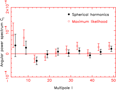
Figure 4: The $C_{\ell}$ spectrum of a model dipole distribution with added multiple-component sources. The spectrum is measured using both spherical harmonic analysis (solid circles) and maximum likelihood estimation (open circles). The measurements were averaged into bands of width $\Delta\ell=5$, starting from $\ell=2$. The results are consistent with $C_{\ell}=0$.

Figure 4 permits a first comparison of the two independent methods of estimating $C_{\ell}$. At low $\ell$, the variances are in excellent agreement. As $\ell$ approaches $2\times n_{\rm side}$, the variance of the maximum likelihood method begins to exceed that of the spherical harmonic analysis. This occurs as the resolution of the pixelization scheme becomes important: the angular pixel size is no longer much less than the characteristic angular scale probed by the $\ell$th multipole. The variance of the high $\ell$ bins could be reduced by adopting a finer pixelization, such as $n_{\rm side}=64$, with the penalty of a rapidly increasing requirement of supercomputer time. Given that the signal in the NVSS angular power spectrum turns out to be confined to $\ell\la 40$, our optimum pixelization remains $n_{\rm side}=32$. Moreover, higher pixel resolution would decrease the mean pixel count $\overline{n}$ in equation 13, rendering a Gaussian distribution a poorer approximation for $x_{i}$.

4 Results

4.1 The angular power spectrum $C_{\ell}$

Figure 5 plots the NVSS angular power spectrum measured for flux-density threshold $S_{\rm 1.4\,GHz}=10$ mJy using both spherical harmonic analysis and maximum likelihood estimation. The constant offset due to double sources (equation 12) has been subtracted and the measurements are averaged into bands of width $\Delta\ell=5$, starting from $\ell_{\rm min}=2$. Measurements are plotted up to $\ell=100$, although note that the variance of the maximum likelihood estimation is increased by pixelization effects above $\ell\sim 50$, as discussed in Section 3.5. Table 1 lists the plotted data. Figure 6 displays the same data scaled by the usual CMB normalization factor, $\ell(\ell+1)/2\pi$.

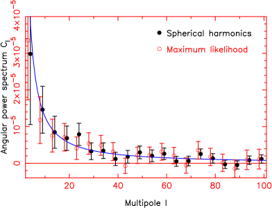
Figure 5: The NVSS $C_{\ell}$ spectrum for a flux-density threshold $S_{\rm 1.4\,GHz}=10$ mJy, determined using two different methods. The $C_{\ell}$ measurements are averaged into bins of width $\Delta\ell=5$, starting from $\ell=2$. The solid circles are the result of a spherical harmonic analysis and the open circles are derived from a maximum likelihood analysis. For clarity, the open circles are offset by $\Delta\ell=-1$. The solid line displays the best-fitting power-law to the spherical harmonic analysis results.

Table 1: Data table of banded NVSS $C_{\ell}$ values plotted in Figure 5. The offset due to double sources is $\Delta C_{\ell}=0.24\times 10^{-5}$.

$\ell_{\rm min}$	$\ell_{\rm max}$	Spherical harmonic	Maximum likelihood
		$C_{\ell}^{\rm obs}\times 10^{5}$	$C_{\ell}^{\rm obs}\times 10^{5}$
2	6	$2.98\pm 1.93$	$3.35\pm 1.62$
7	11	$1.46\pm 0.64$	$1.19\pm 0.64$
12	16	$0.85\pm 0.44$	$0.75\pm 0.45$
17	21	$0.68\pm 0.33$	$0.71\pm 0.38$
22	26	$0.79\pm 0.30$	$0.41\pm 0.31$
27	31	$0.33\pm 0.23$	$0.54\pm 0.29$
32	36	$0.34\pm 0.21$	$0.49\pm 0.27$
37	41	$0.12\pm 0.18$	$0.32\pm 0.25$
42	46	$0.18\pm 0.17$	$-0.07\pm 0.21$
47	51	$0.30\pm 0.17$	$0.22\pm 0.22$
52	56	$0.21\pm 0.16$	$0.22\pm 0.22$
57	61	$0.26\pm 0.16$	$0.31\pm 0.23$
62	66	$0.05\pm 0.14$	$0.21\pm 0.22$
67	71	$0.06\pm 0.13$	$-0.06\pm 0.21$
72	76	$0.25\pm 0.14$	$0.35\pm 0.24$
77	81	$0.13\pm 0.13$	$0.17\pm 0.24$
82	86	$-0.03\pm 0.11$	$0.01\pm 0.24$
87	91	$-0.05\pm 0.11$	$-0.15\pm 0.24$
92	96	$0.08\pm 0.11$	$0.09\pm 0.27$
97	101	$0.12\pm 0.11$	$0.11\pm 0.27$

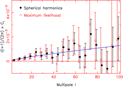
Figure 6: The same data points and power-law fit as Figure 5, scaled by a factor $\ell(\ell+1)/2\pi$ to match the usual CMB convention.

We detect clear signal in the NVSS $C_{\ell}$ spectrum at multipoles $\ell\la 40$, well-fitted by a power-law $C_{\ell}=a\,\ell^{-b}$, where the best-fitting parameters are $a=(2.0\pm 0.4)\times 10^{-4}$, $b=1.20\pm 0.06$ (fitted to the spherical harmonic analysis result) or $a=(1.6\pm 0.4)\times 10^{-4}$, $b=1.12\pm 0.08$ (fitted to the maximum likelihood method result). The amplitude of the angular power spectrum for radio galaxies is two orders of magnitude smaller than that found for optically-selected galaxies (e.g. Huterer, Knox & Nichol 2001); this is readily explained by the wide redshift range of the NVSS sources, which vastly dilutes the clustering signal through the superposition of unrelated redshift slices. The NVSS signal remains $\sim 5$ orders of magnitude greater than the CMB $C_{\ell}$ spectrum over the same multipole range, reflecting the growth of structure since $z=1100$.

Given the incomplete sky and finite resolution, the measured $C_{\ell}$ values are not independent. However, it was argued in Section 3.2 that the correlations between neighbouring power spectrum measurements are small. This fact was confirmed by the maximum likelihood analysis. The degree of correlation between neighbouring bins is given by the immediately off-diagonal elements of the inverse Fisher matrix. This data is generated by the MADCAP software, and inspection revealed that the size of the immediately off-diagonal matrix elements was $\sim 20$ times smaller than that of the diagonal elements.

Figure 7 compares the angular power spectra measured at flux-density thresholds 5 mJy, 10 mJy and 20 mJy using spherical harmonic analysis. The 5 mJy data may be affected by systematic surface density gradients. The results are consistent with an unchanging underlying power spectrum. This is not surprising; the redshift distribution of radio sources does not vary significantly between 5 mJy and 20 mJy, and the angular correlation function has been found not to depend on flux density in this range (Blake & Wall 2002a).

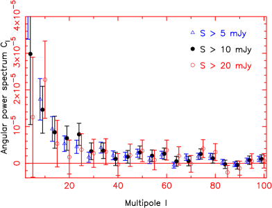
Figure 7: The NVSS $C_{\ell}$ spectrum measured using spherical harmonic analysis for flux-density thresholds of 5 mJy (triangles, $\sigma_{0}=28.2$ deg^-2), 10 mJy (solid circles, $\sigma_{0}=16.9$ deg^-2) and 20 mJy (open circles, $\sigma_{0}=9.5$ deg^-2). The 5 mJy points are offset by $\Delta\ell=-1$ and the 20 mJy points are offset by $\Delta\ell=+1$.

4.2 Probability distribution of $|A_{\ell m}|^{2}$

An interesting probe of the galaxy pattern is the distribution of values of $|A_{\ell m}|^{2}$ (see Hauser & Peebles 1973). These quantities are measured as part of our spherical harmonic analysis (Section 3.2). For a random distribution with surface density $\sigma_{0}$ over a full sky, the central limit theorem ensures that the real and imaginary parts of $A_{\ell m}=\sum_{i}Y_{\ell m}^{*}(i)$ are drawn independently from Gaussian distributions such that the normalization satisfies $|A_{\ell m}|^{2}=\sigma_{0}$. It is then easy to show that $x=|A_{\ell m}|^{2}$ has an exponential probability distribution for $m\neq 0$:

$$P(x)\,dx=\frac{\exp{(-x/\sigma_{0})}}{\sigma_{0}}\,dx$$ (14)

For a partial sky, $|A_{\ell m}|^{2}$ is replaced by $|A_{\ell m}-\sigma_{0}I_{\ell m}|^{2}/J_{\ell m}$ (equation 5).

Figure 8 plots the distribution of observed values of $|A_{\ell m}-\sigma_{0}I_{\ell m}|^{2}/J_{\ell m}$. We restrict this plot to the multipole range $51<\ell<100$: for this range of $\ell$, Figure 5 demonstrates that $C_{\ell}\approx 0$ and thus the survey is well-described by a random distribution with additional multiple components. For each $\ell$ we included the range $1\leq m\leq\ell$ (negative values of $m$ are not independent). Overplotted on Figure 8 as the solid line is the prediction of equation 14. Multiple components cause the slope of the observed exponential distribution to be shallower than this prediction. Section 3.3 shows that the value of $<|A_{\ell m}-\sigma_{0}I_{\ell m}|^{2}/J_{\ell m}>$ is increased from $\sigma_{0}$ to $(1+2e)\sigma_{0}$, where $e$ is the fraction of galaxies split into double sources. Thus equation 14 must be amended such that $P(x)\propto\exp{[-x/(1+2e)\sigma_{0}]}$. Assuming that $e=0.07$, this corrected prediction is plotted on Figure 8 as the dashed line and provides a very good fit to the observed distribution. This is an independent demonstration that approximately 7 per cent of NVSS galaxies are split into multiple-component sources. Figure 8 also underlines the fact that the imprint of clustering on the projected radio sky is very faint.

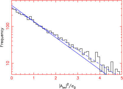
Figure 8: The distribution of values of $|A_{\ell m}|^{2}$ (corrected for partial sky coverage) for the NVSS for $51\leq\ell\leq 100$. The solid line is the prediction for an unclustered galaxy distribution, which should be a good approximation given that $C_{\ell}\approx 0$ for this range in $\ell$. However, the slope is a poor fit due to the influence of multiple-component sources. When these are taken into account, the observed distribution is accurately reproduced (the dashed line).

4.3 Comparison with $w(\theta)$

The angular correlation function $w(\theta)$ has been measured for the NVSS by Blake & Wall (2002a) and Overzier et al. (2003). It is well-described by a power-law $w(\theta)\approx(1\times 10^{-3})\,\theta^{-0.8}$ for angles up to a few degrees. Equation 3 allows us to derive the equivalent $C_{\ell}$ spectrum if we assume that this power-law extends to all angular scales. In Figure 9 we overplot the resulting prediction on the measurements and find an excellent fit.

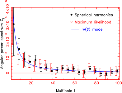
Figure 9: The same data points as Figure 5, overplotted with the prediction of equation 3 assuming an angular correlation function $w(\theta)=(1\times 10^{-3})\,\theta^{-0.8}$.

This is initially surprising: the angular correlation function is only measurable at small angles $\theta<10^{\circ}$, whereas low multipoles $\ell$ describe surface fluctuations on rather larger angular scales. However, in Section 5 we establish that the signal in low multipoles is actually generated at low redshift by spatial fluctuations on relatively small scales, similar to the spatial scales which produce the signal in $w(\theta)$.

Of course the comparison is not entirely straight-forward because the two statistics quantify different properties of the galaxy distribution. The value of $C_{\ell}$ quantifies the amplitude of fluctuations on the angular scale corresponding to $\ell$. The value of $w(\theta)$ is the average of the product of the galaxy overdensity at any point with the overdensity at a point at angular separation $\theta$ – $w(\theta)$ depends on angular fluctuations on all scales. This is illustrated by the inverse of equation 3:

$$w(\theta)=\frac{1}{4\pi\,\sigma_{0}^{2}}\,\sum_{\ell=1}^{\infty}(2\ell+1)\,C_{\ell}\,P_{\ell}(\cos{\theta})$$

For example, a density map constructed using just one multipole $\ell$ possesses a broad angular correlation function.

5 Relation to the spatial power spectrum

The purpose of this Section is to demonstrate that the observed radio galaxy $C_{\ell}$ spectrum can be understood in terms of the current fiducial cosmological model. In Section 6 we utilize this framework to determine the linear bias factor of the radio galaxies, marginalizing over other relevant model parameters.

5.1 Theory

The angular power spectrum $C_{\ell}$ is a projection of the spatial power spectrum of mass fluctuations at different redshifts, $P(k,z)$, where $k$ is a co-moving wavenumber. In linear perturbation theory, fluctuations with different $k$ evolve independently, scaling with redshift according to the growth factor $D(z)$. Under this assumption we can simply scale the present-day matter power spectrum $P_{0}(k)$ back with redshift:

$$P(k,z)=P_{0}(k)\,D(z)^{2}$$ (15)

For an $\Omega_{m}=1$, $\Omega_{\Lambda}=0$ universe, $D(z)=(1+z)^{-1}$. For general cosmological parameters we can use the approximation of Carroll, Press & Turner (1992). If linear theory holds then the angular power spectrum $C_{\ell}$ can be written in terms of the present-day matter power spectrum $P_{0}(k)$ as

$$C_{\ell}=\int\,P_{0}(k)\,W_{\ell}(k)\,dk$$ (16)

(see e.g. Huterer, Knox & Nichol 2001, Tegmark et al. 2002) where the kernel $W_{\ell}(k)$ is given by

$$W_{\ell}(k)=\frac{2}{\pi}\,\left[\int_{0}^{\infty}j_{\ell}(u)\,f(u/k)\,du\right]^{2}$$ (17)

Here, $j_{\ell}$ is a spherical Bessel function and $f(x)$ is a function which depends on the radial distribution of the sources as

$$f(\,x(z)\,)=\frac{p(z)\,D(z)\,b(z)}{dx/dz}$$ (18)

assuming a flat geometry. $x(z)$ is the co-moving radial co-ordinate at redshift $z$, $p(z)$ is the redshift probability distribution of the sources (normalized such that $\int\,p(z)\,dz=1$) and $b(z)$ is a linear bias factor which relates the clustering of galaxies to clustering of the underlying mass:

$$P_{\rm gal}(k,z)=b(z)^{2}P_{\rm mass}(k,z)$$

For the purposes of this analysis we assumed that the linear bias does not evolve with epoch and may be represented by a constant bias factor $b(z)=b_{0}$.

A useful approximation for the spherical Bessel function (which gets better as $\ell$ gets larger) is $j_{\ell}(x)\approx(\pi/2\ell)^{1/2}\,\delta(x-\ell)$. In this approximation,

$$W_{\ell}(k)\approx\frac{1}{\ell}\,f(\ell/k)^{2}$$ (19)

Thus as $\ell$ is increased, the kernel just translates along the $k$-axis. Combining equations 16 and 19 produces the approximation

$$C_{\ell}\approx\frac{1}{\ell}\int\,P_{0}(k)\,f(\ell/k)^{2}\,dk$$ (20)

or, converting this into an integral over radial co-ordinate,

$$C_{\ell}\approx\int\,P_{0}(\ell/x)\,x^{-2}\,f(x)^{2}\,dx$$ (21)

In Section 4.1 we found that the measured NVSS $C_{\ell}$ spectrum was well-fit by a power-law. Inspecting equations 20 and 21, a power law for $C_{\ell}$ can arise in two ways:

• If the function $f(x)$ were a power-law $f(x)\propto x^{n}$, then equation 20 predicts that $C_{\ell}\propto\ell^{\,2n-1}$, regardless of the form of $P_{0}(k)$. In particular, if $f(x)$ were approximately constant over the relevant scales, then $C_{\ell}\propto\ell^{-1}$, which is a good description of the observed NVSS clustering.

• If the spatial power spectrum were a power-law $P_{0}(k)\propto k^{n}$, then equation 21 predicts that $C_{\ell}\propto\ell^{n}$, regardless of the form of the radial distribution $p(z)$ (see also Table 2). The result $C_{\ell}\propto\ell^{n}$ differs from the case of CMB fluctuations, for which $n=1$ corresponds to $C_{\ell}\propto 1/\ell(\ell+1)$ at low $\ell$ – the well-known Sachs-Wolfe effect. This is because the Sachs-Wolfe effect is sensitive to fluctuations in gravitational potential, whereas we are probing fluctuations in mass.

In Section 5.3 we determine that the first of these interpretations is correct.

Table 2: Functional form of common clustering statistics for pure power-law clustering parameterized by slope $\gamma$.

Statistic	Dependence	Validity
Spatial correlation function	$\xi(r)\propto r^{\,-\gamma}$	All $r$
Angular correlation function	$w(\theta)\propto\theta^{\,1-\gamma}$	Small $\theta$
Spatial power spectrum	$P(k)\propto k^{\,\gamma-3}$	All $k$
Angular power spectrum	$C_{\ell}\propto\ell^{\,\gamma-3}$	High $l$

5.2 Modelling the present-day power spectrum

We assumed that the primordial matter power spectrum is a featureless power-law, $P_{\rm prim}(k)=A\,k^{n}$. On very large scales, the only alteration to this spectrum in linear theory will be an amplitude change due to the growth factor. However, during the epoch of radiation domination, growth of fluctuations on scales less than the horizon scale is suppressed by radiation pressure. This process is described by the transfer function $T(k)$, such that the present-day linear matter power spectrum is given by

$$P_{0}(k)=P_{\rm prim}(k)\,T(k)^{2}=A\,k^{n}\,T(k)^{2}$$ (22)

Accurate fitting formulae have been developed for the transfer function $T(k)$ in terms of the cosmological parameters (Eisenstein & Hu 1998), which we employed in our analysis (these fitting formulae assume adiabatic perturbations). In our fiducial cosmological model, we fixed the values of the cosmological parameters at $h=H_{0}/(100{\rm\;km\,s^{-1}\,Mpc^{-1}})=0.73$, $\Omega_{m}h^{2}=0.134$ and $\Omega_{b}/\Omega_{m}=0.17$ (Spergel et al. 2003, Table 7, column 3). We also chose a primordial spectral index $n=0.97$ (Spergel et al. 2003), which is close to the predictions of standard inflationary models. We consider the effect of variations in these parameter values in Section 6. We assumed that the Universe is flat, with the remaining energy density provided by a cosmological constant $\Omega_{\Lambda}=1-\Omega_{m}$.

There are at least two independent ways of estimating the amplitude $A$ in equation 22. Firstly we can use constraints on the number density of massive clusters at low redshift, expressed in terms of $\sigma_{8}$, the rms fluctuation of mass in spheres of radius $R=8\,h^{-1}$ Mpc:

$$\sigma_{R}^{2}=\frac{9}{2\pi^{2}R^{2}}\int P_{0}(k)\,[j_{1}(kR)]^{2}\,dk$$ (23)

For example, Viana & Liddle (1999) determined the most likely value of $\sigma_{8}$ using this method to be $\sigma_{8}=0.56\,\Omega_{m}^{-0.47}$. Alternatively, $A$ can be expressed in terms of the amplitude of fluctuations at the Hubble radius, $\delta_{H}$, and constrained by measurements of CMB anisotropies on large angular scales:

$$A=2\pi^{2}\delta_{H}^{2}\left(\frac{c}{H_{0}}\right)^{3+n}$$ (24)

For example, Bunn & White (1997) give the best-fitting constraint on $\delta_{H}$ and $n$ for flat models ($\Omega_{m}+\Omega_{\Lambda}=1$) based on results of the COBE DMR experiment:

$$\delta_{H}=1.94\times 10^{-5}\,\Omega_{m}^{-0.785-0.05\ln{\Omega_{m}}}e^{-0.95(n-1)-0.169(n-1)^{2}}$$ (25)

with a maximum $1\sigma$ statistical uncertainty of 7 per cent. For our fiducial cosmological parameters, a (reasonably) consistent cosmology is produced if $\sigma_{8}=1$ (i.e. $\delta_{H}=4.7\times 10^{-5}$). We assumed this fiducial normalization in our model, noting that the value of $\sigma_{8}$ is in fact degenerate with the amplitude of a constant linear bias factor $b(z)=b_{0}$.

Equation 22 is only valid ignoring non-linear effects, which will boost the value of $P(k)$ on small scales as modes commence non-linear collapse. We incorporated non-linear corrections using the fitting formula provided by Peacock & Dodds (1996). The resulting model power spectrum is shown in Figure 10. Strictly, this modification violates the assumption of linear evolution implicit in equation 15. However, this is not significant in our analysis because the small scales for which non-linear evolution is important are only significant in the projection at $z\approx 0$.

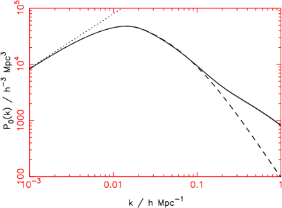
Figure 10: The fiducial model present-day matter power spectrum $P_{0}(k)$ used in this investigation (solid line). This is modified from a primordial featureless power-law (dotted line) using the transfer function of Eisenstein & Hu (1998), and from the linear power spectrum (dashed line) using the non-linear prescription of Peacock & Dodds (1996). The assumed cosmological parameters were $h=0.73$, $\Omega_{m}h^{2}=0.134$, $\Omega_{b}/\Omega_{m}=0.17$, $n=0.97$ and $\sigma_{8,{\rm lin}}=1$.

5.3 Modelling the radial distribution of NVSS sources

The projection of the spatial power spectrum onto the sky depends on the radial distribution of the sources under consideration, which may be deduced from their redshift distribution. We only need to know the probability distribution $p(z)$ of the sources (equation 18), the absolute normalization is not important. Unfortunately, the radial distribution of mJy radio sources is not yet accurately known. The majority of radio galaxies are located at cosmological distances ($z\sim 1$) and their host galaxies are optically very faint.

However, models exist of the radio luminosity function of AGN (i.e. the co-moving space density of objects as a function of radio luminosity and redshift), from which the redshift distribution at any flux-density threshold can be inferred. Such models have been published by Dunlop & Peacock (1990) and Willott et al. (2001). These luminosity function models are by necessity constrained by relatively bright radio sources ($S_{\rm 1.4\,GHz}>100$ mJy) and the extrapolation to NVSS flux-density levels must be regarded as very uncertain. The Willott model is constrained by a larger number of spectroscopic redshifts, and the samples of radio sources used provide fuller coverage of the luminosity-redshift plane (thus the required extrapolation to $S_{\rm 1.4\,GHz}=10$ mJy is less severe). However, the Willott samples are selected at low frequency (151 and 178 MHz), necessitating a large extrapolation to the NVSS observing frequency of 1.4 GHz. The Dunlop & Peacock models are constrained at high frequencies, but treat steep-spectrum and flat-spectrum radio sources as independent populations, which is inconsistent with current ideas concerning the unification of radio AGN (e.g. Jackson & Wall 1999). In addition, they were computed for cosmological parameters $\Omega_{m}=1$, $\Omega_{\Lambda}=0$ rather than the currently favoured “$\Lambda$CDM” cosmology. Furthermore, none of the aforementioned luminosity function models incorporate starburst galaxies, which contribute in significant numbers to the radio galaxy population mix at $z\la 0.1$ for flux-density threshold $S_{\rm 1.4\,GHz}=10$ mJy.

Direct measurements of $p(z)$ are currently only achievable at low redshifts ($z\la 0.2$), where comparison with large optical galaxy redshift surveys is possible (Sadler et al. 2002; Magliocchetti et al. 2002). We matched the NVSS 10 mJy catalogue with the final data release of the 2dF Galaxy Redshift Survey (2dFGRS, available online at http://msowww.anu.edu.au/2dFGRS/, also see Colless et al. 2001), in order to estimate $p(z)$ at low redshift. As our fiducial model, we fitted the resulting redshift histogram with the simplest possible function, a constant $p(z)=p_{0}$ over the range $0<z<0.15$. In Section 6 we include the effect of variations in this model. We only considered the redshift range $z<0.15$ in this analysis because at $z\approx 0.15$, the (very luminous) optical counterparts of the 10 mJy NVSS sources begin slipping below the 2dFGRS magnitude threshold, which we verified by plotting the magnitudes of matched 2dFGRS galaxies against redshift. Having determined the value of $p_{0}$, we created the full redshift distribution by assigning the remaining probability $1-p_{0}$ over the redshift range $z>0.15$ in proportion to the prediction of the Dunlop & Peacock (1990) luminosity function models. For this investigation we used the average of the seven models provided by Dunlop & Peacock. Assuming the Willott et al. (2001) radial distribution for $z>0.15$ made a negligible difference to the results (because most of the contribution to the $C_{\ell}$ spectrum arises at low redshifts, see Section 5.4).

Matching NVSS catalogue entries brighter than $S_{\rm 1.4\,GHz}=10$ mJy with the 2dFGRS database yielded $N_{\rm mat}=546$ identifications with redshifts $z<0.15$, using matching tolerance 10 arcsec (see Sadler et al. 2002). We restricted the 2dFGRS sample to “high quality” spectra ($Q\geq 3$). An estimate of the probability of an NVSS source being located at $z<0.15$ is

$${\rm Prob}=p_{0}\,\Delta z=\frac{N_{\rm mat}/A_{\rm 2dF}}{\sigma_{\rm NVSS}}$$

where $\sigma_{\rm NVSS}=16.9$ deg^-2 is the surface density of NVSS sources brighter than 10 mJy, and $A_{\rm 2dF}$ is the 2dFGRS area under consideration, which (owing to the varying angular completeness) is not trivial to calculate. We followed Sadler et al. (2002) by dividing the number of 2dFGRS galaxies contained in the NVSS geometry by the 2dFGRS surface density $\sigma_{\rm 2dF}=180$ deg^-2, resulting in an effective area $A_{\rm 2dF}=1214$ deg².

The result, $p_{0}=0.177$ (per unit redshift), is a significant underestimate for various reasons:

• Incompletenesses in the 2dFGRS input catalogue ($5\%$).

• Input catalogue galaxies unable to be assigned a 2dF spectrograph fibre ($7\%$).

• Observed 2dFGRS spectra with insufficient quality ($Q\leq 2$) to determine a redshift ($8\%$).

• Extended radio sources with catalogue entries located more than 10 arcsec from the optical counterpart ($3\%$).

The estimated correction factors in brackets were obtained from Colless et al. (2001) and from Carole Jackson (priv. comm.). Multiplying these corrections implies a total incompleteness of $25\%$, and on this basis we increased the value of $p_{0}$ to $0.177/0.75=0.237$.

Figure 11 plots 2dFGRS-NVSS matches in redshift bins of width $\Delta z=0.01$, together with the low-redshift fit described above. A constant $p(z)$ is a fairly good approximation at low redshifts ($z<0.15$). This flat distribution arises because the overall redshift distribution is a sum of that due to AGN and that due to starburst galaxies; $p(z)$ increases with $z$ for the AGN, but decreases with $z$ for the starbursters. Figure 11 also displays the predictions of the luminosity function models of Dunlop & Peacock (1990) and Willott (2001). As explained above, the large extrapolations involved render these models a poor fit to the redshift distribution at mJy flux levels, and their use without modification at low redshift would have caused significant error.

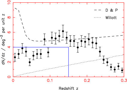
Figure 11: The redshift distribution $dN/dz$ of NVSS sources brighter than 10 mJy. The data points are measured values resulting from cross-matching with the 2dF Galaxy Redshift Survey, and the solid line is the best-fitting constant $dN/dz=p_{0}\times\sigma_{\rm NVSS}$ for $0<z<0.15$. We also plot the predictions of two luminosity-function models: Dunlop & Peacock (1990, dashed line) and Willott et al. (2001, dotted line). The NVSS-2dFGRS matches decline at $z\ga 0.2$ due to the falling $dN/dz$ of the optical catalogue.

5.4 Predicting the $C_{\ell}$ spectrum

We used equation 16 to predict the $C_{\ell}$ spectrum from our fiducial models of the spatial power spectrum (Section 5.2) and the radial distribution of the sources (Section 5.3). We found that a good match to the measured angular power spectrum resulted if the NVSS sources were assigned a constant linear bias factor $b_{0}\approx 1.7$ (Figure 12); $b_{0}=1$ provides a very poor fit to the results. The bias factor of the radio galaxies is analyzed more thoroughly in Section 6.

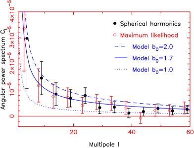
Figure 12: The predicted $C_{\ell}$ spectrum for NVSS sources brighter than 10 mJy from a reasonable model spatial power spectrum (Section 5.2) and model redshift distribution (Section 5.3). The amplitude of the measurements can only be matched if radio galaxies are assigned a high bias; model predictions are plotted for constant linear bias factors $b_{0}=1$ (dotted line), $b_{0}=1.7$ (solid line) and $b_{0}=2$ (dashed line).

We note that these measurements of the radio galaxy $C_{\ell}$ spectrum at low $\ell$ are not directly probing the large-scale, small $k$, region of the power spectrum $P(k)$. Investigation of the integrands of equations 20 and 21 revealed that the majority of the signal is built up at low redshift, $z\la 0.1$ (see Figure 13), where small-scale spatial power is able to contribute on large angular scales (i.e. contribute to low multipoles). Higher redshift objects principally serve to dilute the clustering amplitude. This is unfortunate: the potential of radio galaxies distributed to $z\sim 1$ to probe directly the large-scale power spectrum is forfeited by projection effects. In order to realize this potential, we must measure redshifts for the NVSS sources. A three-dimensional map extending to $z\sim 1$ would directly yield $P(k)$ on large scales, defining the “turn-over” sketched in Figure 10.

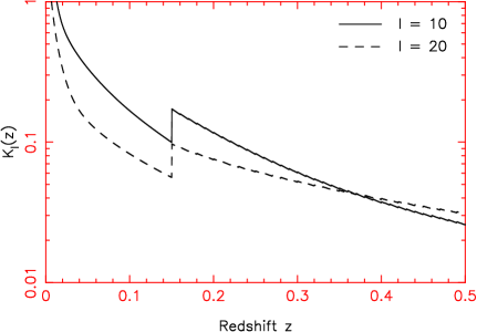
Figure 13: Contribution to the model NVSS angular power spectrum as a function of redshift for multipoles $\ell=10$ (solid line) and $\ell=20$ (dashed line), derived from equation 21 using the assumptions detailed in Sections 5.2 and 5.3. The Figure plots $K_{\ell}(z)$ where $C_{\ell}=\int K_{\ell}(z)\,dz$. The $y-$axis in the Figure is scaled arbitrarily. The discontinuity at $z=0.15$ results from the break in the model $p(z)$ at this redshift (see Section 5.3).

6 Radio galaxy bias factor

The enhanced radio galaxy bias apparent in Figure 12 is consistent with the nature of AGN host galaxies: optically luminous ellipticals inhabiting moderate to rich environments. Similarly high radio galaxy bias factors have been inferred from measurements of the spatial power spectrum of low-redshift radio galaxies (Peacock & Dodds 1994) and from deprojection of the NVSS angular correlation function $w(\theta)$ (Blake & Wall 2002a; Overzier et al. 2003). Furthermore, Boughn & Crittenden (2002) cross-correlated NVSS and CMB overdensities in a search for the Integrated Sachs-Wolfe effect (see also Nolta et al. 2003). Their analysis included fitting theoretical models to the NVSS angular correlation function. They derived good fits for a slightly lower linear bias factor than ours, $b_{0}=1.3\rightarrow 1.6$. This difference is due to the assumed redshift distribution. Boughn & Crittenden also used the Dunlop & Peacock (1990) average model, but we corrected this model using observational data at low redshifts $z<0.15$. As can be seen from Figure 11, our correction reduces the number of low-redshift sources, necessitating a higher bias factor to recover the same angular correlations.

In order to derive a formal confidence interval for the linear bias parameter $b_{0}$ we must incorporate the effects of uncertainties in the underlying model parameters (by marginalizing over those parameters). With this in mind, we assumed Gaussian priors for Hubble’s constant $h=0.73\,\pm\,0.03$, for the matter density $\Omega_{m}h^{2}=0.134\,\pm\,0.006$, and for the primordial spectral index $n=0.97\,\pm\,0.03$. The widths of these priors were inspired by the cosmological parameter analysis combining the WMAP satellite observations of the CMB and the 2dFGRS galaxy power spectrum (Spergel et al. 2003, Table 7, column 3) and are a good representation of our current knowledge of the cosmological model. In addition, we considered variations in the model for the radial distribution of NVSS sources at low redshift (Section 5.3), using a more general fitting formula $p(z)=a+b\,z$ to describe the probability distribution for $z<0.15$. For each pair of values of $(a,b)$ we derived the chi-squared statistic between the model and the observations, $\chi^{2}_{p(z)}$, which we converted into an (unnormalized) probability density $P_{p(z)}\propto\exp{(-\chi^{2}_{p(z)}/2)}$.

Our model is thus specified by values of ($b_{0}$, $h$, $\Omega_{m}h^{2}$, $n$, $a$, $b$) from which we can calculate a model $C_{\ell}$ spectrum and hence a chi-squared statistic with the observations, $\chi^{2}_{C_{\ell}}$, corresponding to a probability density $P_{C_{\ell}}\propto\exp{(-\chi^{2}_{C_{\ell}}/2)}$. We used the spherical harmonic estimation of the $C_{\ell}$ spectrum as the observational data. After multiplying $P_{C_{\ell}}$ by the redshift distribution probability density $P_{N(z)}(a,b)$ and the Gaussian prior probability densities for $h$, $\Omega_{m}h^{2}$ and $n$, we derived the probability distribution for $b_{0}$ by integrating over each of the other parameters. We do not marginalize over the normalization of the matter power spectrum, $\sigma_{8}$, because this quantity is degenerate with $b_{0}$ (using equations 18, 21 and 23: $C_{\ell}\propto b_{0}^{2}\,\sigma_{8}^{2}$).

The resulting normalized probability distribution for $b_{0}\times\sigma_{8}$ is displayed in Figure 14, from which we determined a $68\%$ confidence region $b_{0}\,\sigma_{8}=1.53\rightarrow 1.87$. When combined with the WMAP determination of $\sigma_{8}=0.9\pm 0.1$ (Spergel et al. 2003), we infer that $b_{0}=1.89\pm 0.27$.

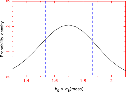
Figure 14: Normalized probability distribution for $b_{0}\times\sigma_{8}$, obtained after marginalizing over the other parameters of the model as described in Section 6. The bounds of the $68\%$ confidence region are marked by the vertical dashed lines.

7 Conclusions

This investigation has measured the angular power spectrum of radio galaxies for the first time, yielding consistent results through the application of two independent methods: direct spherical harmonic analysis and maximum likelihood estimation. The NVSS covers a sufficient fraction of sky ($\sim 80$ per cent) that spherical harmonic analysis is very effective, with minimal correlations amongst different multipoles. The form of the $C_{\ell}$ spectrum can be reproduced by standard models for the present-day spatial power spectrum and for the radial distribution of NVSS sources – provided that this latter is modified at low redshift through comparison with optical galaxy redshift surveys. The results strongly indicate that radio galaxies possess high bias with respect to matter fluctuations. A constant linear bias $b_{0}\approx 1.7$ permits a good fit, and by marginalizing over the other parameters of the model we deduce a $68\%$ confidence interval $b_{0}\,\sigma_{8}=1.53\rightarrow 1.87$ where $\sigma_{8}$ describes the normalization of the matter power spectrum. We find that the majority of the angular power spectrum signal is generated at low redshifts, $z\la 0.1$. Therefore, in order to exploit the potential of radio galaxies to probe spatial fluctuations on the largest scales, we require individual redshifts for the NVSS sources.

References

- [1] Baleisis A., Lahav O., Loan A.J., Wall J.V., 1998, MNRAS, 297, 545
- [2] Becker R.H., White R.L., Helfand D.J., 1995, ApJ, 450, 559
- [3] Blake C.A., Wall J.V, 2002a, MNRAS, 329, L37
- [4] Blake C.A., Wall J.V, 2002b, Nature, 416, 150
- [5] Bond J.R., Jaffe A.H., Knox L., 1998, PhRvD, 57, 2117
- [6] Bond J.R., Efstathiou G., Tegmark M., 1997, MNRAS, 291, 33
- [7] Borrill J., 1999, in Proceedings of the 5th European SGI/Cray MPP Workshop (astro-ph/9911389)
- [8] Boughn S.P., Crittenden R.G., 2002, PhRvL, 88, 1302
- [9] Brand K., Rawlings S., Hill G.J., Lacy M., Mitchell E., Tufts J., 2003, MNRAS, 344, 283
- [10] Bunn E.F., White M., 1997, ApJ, 480, 6
- [11] Carroll S.M., Press W.H., Turner E.L., 1992, ARA&A, 30, 499
- [12] Colless M. et al., 2001, MNRAS, 328, 1039
- [13] Condon J., Cotton W., Greisen E., Yin Q., Perley R., Taylor G., Broderick J., 1998, AJ, 115, 1693
- [14] Cress C., Helfand D., Becker R., Gregg M., White R., 1996, ApJ, 473, 7
- [15] Dunlop J.S., Peacock J.A., 1990, MNRAS, 247, 19
- [16] Efstathiou G., Moody S., 2001, MNRAS, 325, 1603
- [17] Eisenstein D.J., Hu W., 1998, ApJ, 496, 605
- [18] Gorski K.M., Hivon E., Wandelt B.D., 1999, in Proceedings of the MPA/ESO Cosmology Conference “Evolution of Large-Scale Structure”, p.37 (astro-ph/9812350)
- [19] Hauser M.G., Peebles P.J.E., 1973, ApJ, 185, 757
- [20] Hill G.J., Lilly S.J., 1991, ApJ, 367, 1
- [21] Huterer D., Knox L., Nichol R.C., 2001, ApJ, 555, 547
- [22] Jackson C.A., Wall J.V., 1999, MNRAS, 304, 160
- [23] Magliocchetti M., Maddox S., Lahav O., Wall J., 1998, MNRAS, 300, 257
- [24] Magliocchetti M. et al., 2002, MNRAS, 333, 100
- [25] Nolta et al., 2003, ApJ submitted (astro-ph/0305097)
- [26] Overzier R.A., Röttgering H.J.A., Rengelink R.B., Wilman R.J., 2003, A&A, 405, 53
- [27] Peacock J.A., Dodds S.J., 1994, MNRAS, 267, 1020
- [28] Peacock J.A., Dodds S.J., 1996, MNRAS, 280, 19
- [29] Peebles P.J.E., 1973, ApJ, 185, 413
- [30] Sadler E.M. et al., 2002, MNRAS, 329, 227
- [31] Scott D., Srednicki M., White M., 1994, ApJ, 421, 5
- [32] Spergel D.N. et al. 2003, ApJS, 148, 175
- [33] Tegmark M. et al., 2002, ApJ, 571, 191
- [34] Viana P.T.P., Liddle A.R., 1999, MNRAS, 303, 535
- [35] Wandelt B.D., Hivon E., Gorski K.M., 2001, PhRvD, 64, 3003
- [36] Willott C.J., Rawlings S., Blundell K.M., Lacy M., Eales S.A., 2001, MNRAS, 322, 536
- [37] Wright E.L., Smoot G.F., Bennett C.L., Lubin P.M., 1994, ApJ, 436, 441