Observing the build–up of the colour-magnitude relation at redshift $\sim 0.8$

Abstract

We analyse the rest–frame (U$-$V) colour–magnitude relation for $2$ clusters at redshift $0.7$ and $0.8$, drawn from the ESO Distant Cluster Survey. By comparing with the population of red galaxies in the Coma cluster, we show that the high redshift clusters exhibit a deficit of passive faint red galaxies. Our results show that the red–sequence population cannot be explained in terms of a monolithic and synchronous formation scenario. A large fraction of faint passive galaxies in clusters today has moved onto the red sequence relatively recently as a consequence of the fact that their star formation activity has come to an end at $z<0.8$.

1 Introduction

Red cluster galaxies form a tight sequence in the colour–magnitude diagram that, in nearby clusters, extends over a range of at least $5$–$6$ mag from the Brightest Cluster Galaxy (BCG). The existence of a tight colour–magnitude relation (CMR) up to redshift $\sim 1$, and the evolution of its slope and its zero–point as a function of redshift, are commonly interpreted as the result of a single formation scenario in which cluster ellipticals constitute a passively evolving population formed at high redshift ($z\gtrsim 2$–$3$) in a monolithic collapse ([Kodama et al. (1998), Kodama et al. 1998]). In this model, the slope of the CMR reflects metallicity differences and naturally arises taking into account the effects of supernovae winds. An alternative explanation has been proposed by [Kauffmann & Charlot (1998)] and confirmed recently by [De Lucia, Kauffmann & White (2004)]. In this model, elliptical galaxies form through mergers of disk systems and a CMR arises because more massive ellipticals form by mergers of more massive, and hence more metal rich, disk systems.

On the other hand, it is clear that red passive galaxies in distant clusters constitute only a subset of the passive galaxy population in clusters today ([van Dokkum & Franx (1996), van Dokkum & Franx 1996]). Distant clusters contain significant populations of galaxies with active star formation, that can evolve onto the CMR after their star formation activity is terminated, possibly as a consequence of their infall onto clusters ([Smail et al. (1998), Poggianti et al. (1999), Smail et al. 1998; Poggianti et al. 1999]).

In this work we present the CMR for $2$ clusters at redshifts $0.7$ and $0.8$ from the ESO Distant Cluster Survey (EDisCS).

2 The ESO Distant Cluster Survey

EDisCS is an ESO Large Programme aimed at the study of cluster structure and cluster galaxy evolution over a significant fraction of cosmic time. It will provide homogeneous photometry and spectroscopy for $10$ clusters at redshift $\sim 0.4-0.5$ and $10$ clusters at redshift $\sim 0.7-0.8$.

In this work we present results for $2$ clusters at redshift $0.7$ (cl$1054.4$–$1146$) and $0.8$ (cl$1216.8$–$1201$). The clusters have been imaged in V, R, and I with FORS2 at the ESO’s Very Large Telescope. The average integration times used were $115$ m in the I–band, and $120$ m in the V–band. Multi–object spectroscopy was carried out using FORS2 on the VLT. All data and details about their analysis will be presented in forthcoming papers (White et al, Halliday et al., in preparation; see also Halliday et al., these proceedings). Objects detection has been performed using SExtractor ([Bertin & Arnouts (1996), Bertin & Arnouts 1996]) in ‘two–image’ mode using the I–band images as detection reference images. In the following, we will use magnitude and colours measured on the seeing–matched (to $0.8$ arcsec – our ‘worst’ seeing) registered frames using a fixed circular aperture with $1$ arcsec radius. At the clusters redshifts, this aperture corresponds to a physical radius of $7.13$–$7.50$ kpc (we use $\Omega_{\rm m}=0.3$, $\Omega_{\Lambda}=0.7$, and $H_{0}=70\,{\rm km}\,{\rm s}^{-1}\,{\rm Mpc}^{-1}$).

3 Method and Results

We have computed photometric redshifts using two independent codes (see [Rudnick et al. (2003), Rudnick et al. 2003]) and we have rejected non–members using a two–step procedure: (i) we use the full redshift probability distributions from the codes to isolate objects with high probability to be at the cluster redshift and (ii) we perform a statistical subtraction on the remaining objects using the distribution on the CMR of all the objects at distance from the BCG larger than $1$ Mpc.

Fig. 1 (panels a and b) shows the V$-$I diagram for the $2$ clusters used in this analysis. At these redshifts, V$-$I approximatively samples the rest–frame U$-$V colour, and is therefore very sensitive to any recent or ongoing star formation episode. A red sequence is clearly visible for each cluster, together with a significant population of the blue galaxies known to populate clusters at high redshift. Thin solid lines correspond to $3$ and $5\sigma$ detection limits in the V–band. Empty symbols represent galaxies retained as cluster members; filled circles and crosses are spectroscopically confirmed members with absorption and emission–line spectra respectively. Panel (c) of Fig. 1 shows the U$-$V CMR for the Coma cluster including all galaxies in the catalogue by [Terlevich, Caldwell & Bower (2001)]. Here we use magnitudes and colours in a $25.2$ arcsec diameter aperture that, at the redshift of Coma, corresponds to a physical size of $11.71$ kpc and therefore quite closely approximates our $\sim 14$ kpc diameter aperture at $z=0.8$. We have assumed a distance modulus of $35.16$ and converted observed colours to rest–frame colours using tabulated K–corrections ([Poggianti (1997), Poggianti 1997]).

The green boxes in Fig. 1 show the location of a model with a single burst at $z=3$, and the red diamonds show the location of a model with a $1$ Gyr exponentially declining SFR starting at $z=3$, calculated with the code by [Bruzual & Charlot (2003)]. Three different metallicities are shown: $0.02$, $0.008$ and $0.004$ (from brighter to fainter). The single burst model provides a remarkably good fit to the CMR of the high redshift clusters, confirming that the location of the CM sequence observed in distant clusters requires high redshifts of formation, and that the slope is consistent with a correlation between galaxy metal content and luminosity.

However, Fig. 1 also shows that the CMR in our clusters is strikingly ‘empty’ at magnitudes fainter than $\sim 23$. In order to quantify this effect, we compute the luminosity function (LF) of red sequence galaxies. Fig. 2 shows the numbers of bona fide cluster members within $\sim 3\sigma$ from the best fit relation as a function of galaxy magnitudes. For the EDisCS clusters, we combine the results for the $2$ clusters correcting colours and magnitudes to a common redshift $=0.75$ and average over $100$ realizations of the statistical subtraction for each cluster. For Coma, we have corrected the number of red galaxies in each magnitude bin for background and foreground contamination using a redshift catalogue kindly provided by Matthew Colless and the same procedure as in [Mobasher et al. (2003)].

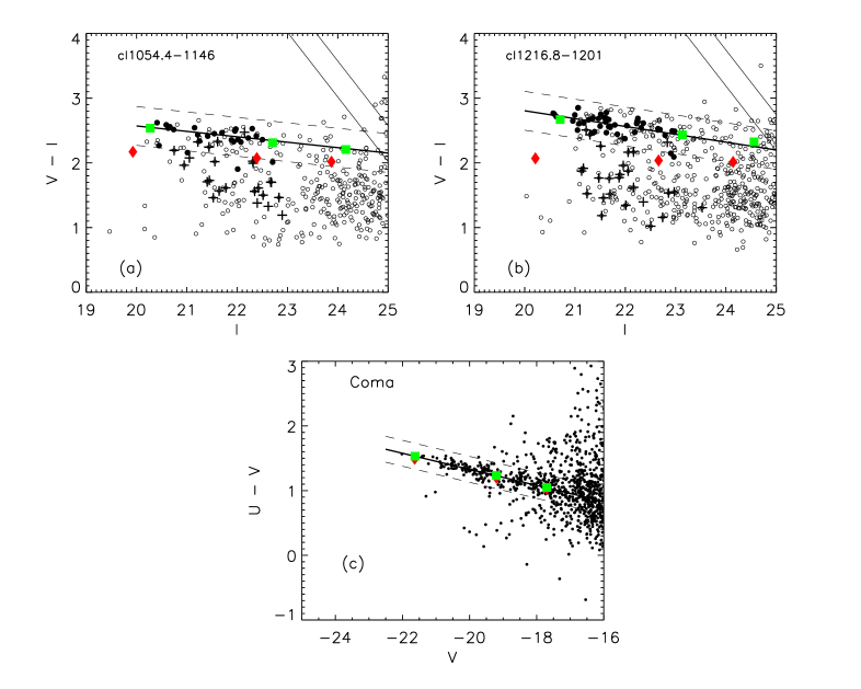
Figure 1: CM diagrams for the $2$ EDisCS clusters under investigation (panels a and b) and for the Coma cluster (panel c). The solid thick line represents the best fit relation measured using a bi–weight estimator and only the spectroscopic members with absorption spectra. The dashed lines correspond to $\pm 3\sigma$ from the best fit, where $\sigma$ is the dispersion of the objects used for the fit. Boxes and diamonds show the location of models with different star formation histories (see text for detail). [See online version of the proceeding book for a colour version of this figure].

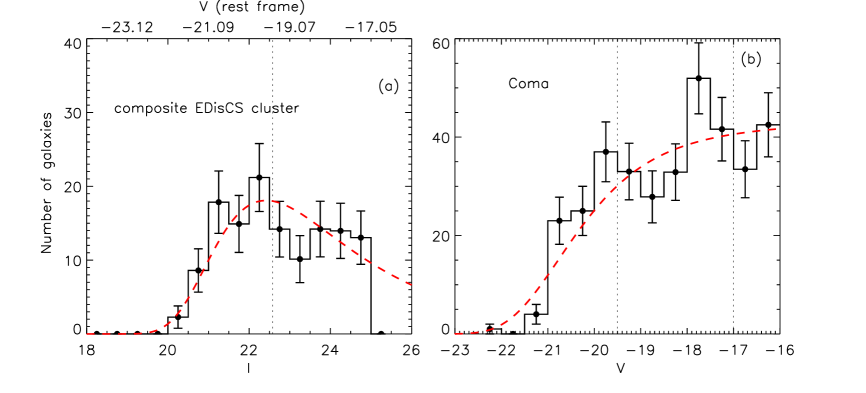
Figure 2: LF of red-sequence galaxies for a composite cluster at redshift $0.75$ (panel a) and for the Coma cluster (panel b). Poisson error bars are shown. The dashed lines represent a fit with a Schechter function. The scale on the top of the left panel has been obtained from the observed I–band magnitudes after correcting for passive evolution. Dotted vertical lines show the limits used to define the luminous–to–faint ratio (see text for detail).

The histogram of the EDisCS clusters shows a remarkable deficiency of $\lesssim 0.1$L_∗ red sequence galaxies. In contrast, the number of passive red galaxies in Coma tends to increase going to fainter magnitudes, in agreement with the luminosity function of early spectral types in clusters in the 2dF Galaxy Redshift Survey ([De Propros et al. (2003), De Propris et al. 2003]). A Schechter fit to the histograms shown in Fig. 2 yields a faint–end slope of $-0.82$ for the EDisCS clusters and $-1$ for Coma, but the error bars are quite large and therefore the results of the fit are just indicative.

If we arbitrarily classify as ‘luminous’ galaxies those brighter than $M_{\rm V}=-19.5$ (this corresponds to an observed I–band magnitude of $22.57$ at redshift $0.75$), and as ‘faint’ those galaxies that are fainter than this magnitude and brighter than $-17$ (this corresponds to the magnitude limit for our high redshift clusters), we obtain a luminous–to–faint ratio for the Coma cluster $0.48\pm 0.06$, where the error has been estimated assuming a Poisson statistics. The corresponding value for the composite EDisCS cluster is $0.99\pm 0.17$. This ratio therefore differs between the composite high redshift cluster and the Coma cluster at about a $3\sigma$ level.

4 Discussion and Conclusions

The results presented are robust both against the technique adopted for removing non–cluster members and against the photometric errors. The red galaxy deficit is detected also when rejecting non–members using a purely statistical subtraction or a more stringent criterion for membership based solely on photometric redshifts. In fact, a deficit is evident also in the full photometric catalogue, when no field correction is attempted. Photometric errors in the EDisCS catalogue are comparable to the errors for the Coma data, therefore the differences observed in the distributions of Fig. 2 cannot be a spurious result arising from photometric errors.

A decline in the number of red sequence members at faint magnitudes was first observed in clusters at $z=0.25$ by [Smail et al. (1998)]. Evidence for a ‘truncation’ of the CM sequence has been noticed in a cluster at $z=1.2$ by [Kajisawa et al. (2000)], who suggested that faint early–type galaxies might not have been in place until $z\sim 1.2$. In more recent work [Kodama et al. (2004)] have come to the same conclusion using deep wide-field optical imaging data of the Subaru/XMM-Newton Deep Survey.

The CMR of the $2$ EDisCS clusters at $z\sim 0.8$ also shows a deficit of red, relatively faint galaxies. Our investigation shows that the evolution of the red–sequence population at these redshifts cannot be explained as the result of a monolithic and synchronous formation scenario. A large fraction of the passive $\lesssim 0.1$L_∗ galaxies must have moved onto the CMR at redshifts lower than $0.8$ as a consequence of the fact that their star formation activity has come to an end. Our analysis enlightens the importance of studying the evolution of the cluster population as a whole, trying to understand how galaxies are accreted from the field, how the dense cluster environment affects their star formation rate, and how these galaxies fade and move on to the red sequence. Only this kind of analysis can unveil the full evolutionary paths of galaxies that lie on the red–sequence today and give strong constraints on the relative importance of star formation and metallicity in establishing the the observed red–sequence. We plan to investigate this in more detail in future work.