Probing Dark Matter Haloes with Satellite Kinematics

Abstract

Using detailed mock galaxy redshift surveys we investigate to what extent the kinematics of large samples of satellite galaxies extracted from flux-limited surveys can be used to constrain halo masses. Unlike previous studies, which focussed only on satellites around relatively isolated host galaxies, we try to recover the average velocity dispersion of satellite galaxies in all haloes, as a function of the luminosity of the host galaxy. We show that previous host-satellite selection criteria yield relatively large fractions of interlopers and with a velocity distribution that, contrary to what has been assumed in the past, differs strongly from uniform. We show that with an iterative, adaptive selection criterion one can obtain large samples of hosts and satellites, with strongly reduced interloper fractions, that allow an accurate measurement of $\sigma_{\rm sat}(L_{\rm host})$ over two and a half orders of magnitude in host luminosity. We use the conditional luminosity function (CLF) to make predictions, and show that satellite weighting, which occurs naturally when stacking many host-satellite pairs to increase signal-to-noise, introduces a bias towards higher $\sigma_{\rm sat}(L_{\rm host})$ compared to the true, host-averaged mean. A further bias, in the same direction, is introduced when using flux-limited, rather than volume-limited surveys. We apply our adaptive selection criterion to the 2dFGRS and obtain a sample of 12569 satellite galaxies and 8132 host galaxies. We show that the kinematics of these satellite galaxies are in excellent agreement with the predictions based on the CLF, after taking account of the various biases. We thus conclude that there is independent dynamical evidence to support the mass-to-light ratios predicted by the CLF formalism.

1 Introduction

Ever since the “discovery” of dark matter astronomers have attempted to obtain accurate measurements of the masses of the extended dark matter haloes in which galaxies are thought to reside. A detailed knowledge of halo masses around individual galaxies holds important clues to the physics of galaxy formation, and is an essential ingredient of any successful model that aims at linking the observable Universe (i.e., galaxies) to the bedrock of our theoretical framework (i.e. dark matter).

The main challenge in measuring total halo masses is to find a suitable, visible tracer at sufficiently large radii in the halo potential well. Traditionally, starting with the actual discovery of evidence for dark matter by Zwicky (1933, 1937), astronomers have used the kinematics of satellite galaxies. Since the number of detectable satellites in individual systems is generally small, this technique is basically limited to clusters of galaxies (e.g., Carlberg et al. 1996; Carlberg, Yee & Ellingson 1997b) and the local group (e.g., Little & Tremaine 1987; Lin, Jones & Klemola 1995; Evans & Wilkinson 2000; Evans et al. 2000). However, one can stack the data on many host-satellite pairs to obtain statistical estimates of halo masses. Pioneering efforts in this direction were made by Erickson, Gottesman & Hunter (1987), Zaritsky et al. (1993, 1997), and Zaritsky & White (1994). Although these studies were typically limited to samples of less than 100 satellites, they nevertheless sufficed to demonstrate the existence of extended massive dark haloes around (spiral) galaxies.

More recently, large, homogeneous galaxy surveys, such as the Sloan Digital Sky Survey (SDSS; York et al. 2000) and the Two Degree Field Galaxy Redshift Survey (2dFGRS; Colless et al. 2001) have dramatically improved both the quantity and quality of data on (nearby) galaxies, thus allowing the construction of much larger samples of host-satellite pairs (McKay et al. 2002; Prada et al. 2003; Brainerd & Specian 2003). Yet, each of these studies has been extremely conservative in their selection of “isolated” hosts and “tracer” satellites. For example, McKay et al. (2002), Prada et al. (2003) and Brainerd & Specian (2003) used samples with 1225, 2734, and 2340 satellites, respectively. For comparison, the SDSS and 2dFGRS, from which these samples were selected, contain well in excess of one hundred thousand galaxies. The main reason for being so conservative is to prevent too large numbers of interlopers (i.e., satellites that are not bound to their host galaxies, but only appear associated because of projection effects). In addition, the selection criteria are optimized to only select isolated galaxies, with the motivation that the dynamics of binary systems, for example, are more complicated.

In this paper we use a different approach and investigate to what extent the kinematics of satellite galaxies may be used to estimate the mean mass-to-light ratio, averaged over all possible dark matter haloes. We make the simple ansatz that satellite galaxies are in virial equilibrium within their dark matter potential well. This is motivated by the finding that dark matter subhaloes, which are likely to be associated with satellite galaxies, have indeed been found to be in a steady-state equilibrium (Diemand, Moore & Stadel 2004). Although we acknowledge that not all systems will be fully virialized, we hypothesize that with a sufficiently large sample of hosts and satellites the assumption of virial equilibrium is sufficiently accurate to describe the mean properties. We use detailed mock galaxy redshift surveys (hereafter MGRSs) to optimize the selection criteria for host and satellite galaxies and show that an iterative, adaptive selection criterion is ideal to limit the number of interlopers while still yielding large numbers of hosts and satellites. Applying our selection criteria to the 2dFGRS yields 8132 hosts with 12569 satellites. We show that the kinematics of these satellite galaxies are in good agreement with predictions based on the conditional luminosity function introduced by Yang, Mo & van den Bosch (2003a) and van den Bosch, Yang & Mo (2003a).

This paper is organized as follows. In Section 2 we first describe, in detail, the construction of our MGRSs. In Section 3 we use these MGRSs to compare three different selection criteria for host and satellite galaxies. We investigate the impact of interlopers and non-central hosts on the satellite kinematics, and show how stacking data from flux-limited surveys results in a systematic overestimate of the true average velocity dispersion of satellite galaxies. We show how the CLF can be used to take these biases into account. In Section 4 we apply our selection criteria to the 2dFGRS and compare the results to analytical estimates and to our MGRS. We summarize our findings in Section 5.

Throughout we assume a flat $\Lambda$CDM cosmology with $\Omega_{m}=0.3$, $\Omega_{\Lambda}=0.7$, $h=H_{0}/(100\>{\rm km}\,{\rm s}^{-1}\,{\rm Mpc}^{-1})=0.7$ and with initial density fluctuations described by a scale-invariant power spectrum with normalization $\sigma_{8}=0.9$.

2 Mock Galaxy Redshift Surveys

What is the best way to select host and satellite galaxies from redshift surveys such as the 2dFGRS and the SDSS? How does the flux-limited nature of these surveys impact on the results? How do interlopers bias the mass estimates? In order to address these and other questions we use detailed mock galaxy redshift surveys. These have the advantage that (i) we know exactly the input mass-to-light ratios that we aim to recover, (ii) we can mimic realistic host/selection criteria and investigate the impact of interlopers. In addition, MGRSs allow a detailed investigation of the effect of Malmquist bias, various survey incompleteness effects, boundary effects due to the survey geometry, etc.

To construct MGRSs two ingredients are required; a distribution of dark matter haloes and a description of how galaxies of different luminosity occupy haloes of different mass. For the former we use large numerical simulations (see Section 2.1 below), and for the latter the conditional luminosity function $\Phi(L|M){\rm d}L$. The conditional luminosity function (hereafter CLF) was introduced by Yang et al. (2003a) and van den Bosch et al. (2003a) as a statistical tool to link galaxies to their dark matter haloes, and describes the average number of galaxies with luminosity $L\pm{\rm d}L/2$ that reside in a halo of mass $M$. As shown in these papers, the CLF is well constrained by the 2dFGRS luminosity function of Madgwick et al. (2002) and the correlation lengths as a function of luminosity obtained by Norberg et al. (2002a). Details about the CLF used in this paper can be found in Appendix A.

2.1 Numerical Simulations

The distribution of dark matter haloes is obtained from a set of large $N$-body simulations (dark matter only) for a $\Lambda$CDM ‘concordance’ cosmology with $\Omega_{m}=0.3$, $\Omega_{\Lambda}=0.7$, $h=0.7$ and $\sigma_{8}=0.9$. The set consists of a total of six simulations with $N=512^{3}$ particles each, and is described in more detail in Jing (2002) and Jing & Suto (2002). All simulations consider boxes with periodic boundary conditions; in two cases $L_{\rm box}=100h^{-1}\>{\rm Mpc}$ while the other four simulations all have $L_{\rm box}=300h^{-1}\>{\rm Mpc}$. Different simulations with the same box size are completely independent realizations and are used to estimate uncertainties due to cosmic variance. The particle masses are $6.2\times 10^{8}\>h^{-1}\rm M_{\odot}$ and $1.7\times 10^{10}\>h^{-1}\rm M_{\odot}$ for the small and large box simulations, respectively. In what follows we refer to simulations with $L_{\rm box}=100h^{-1}\>{\rm Mpc}$ and $L_{\rm box}=300h^{-1}\>{\rm Mpc}$ as $L_{100}$ and $L_{300}$ simulations, respectively.

Dark matter haloes are identified using the standard friends-of-friends algorithm (Davis et al. 1985) with a linking length of $0.2$ times the mean inter-particle separation. For each individual simulation we construct a catalogue of haloes with $10$ particles or more, for which we store the mass, the position of the most bound particle, and the halo’s mean velocity and velocity dispersion. Haloes that are unbound are removed from the sample. In Yang et al. (2003b) we have shown that the resulting halo mass functions are in excellent agreement with the analytical halo mass function given by Sheth, Mo & Tormen (2001a) and Sheth & Tormen (2002).

2.2 Halo Occupation Numbers

Because of the mass resolution of the simulations and because of the completeness limit of the 2dFGRS we adopt a minimum galaxy luminosity of $L_{\rm min}=3\times 10^{7}h^{-2}\>{\rm L_{\odot}}$ throughout. The mean number of galaxies with $L\geq L_{\rm min}$ that resides in a halo of mass $M$ follows from the CLF according to:

$$\langle N\rangle_{M}=\int_{L_{\rm min}}^{\infty}\Phi(L|M)\,{\rm d}L\,.$$ (1)

In order to Monte-Carlo sample occupation numbers for individual haloes one requires the full probability distribution $P(N|M)$ (with $N$ an integer) of which $\langle N\rangle_{M}$ gives the mean, i.e.,

$$\langle N\rangle_{M}=\sum_{N=0}^{\infty}N\,P(N|M)$$ (2)

We use the results of Kravtsov et al. (2003), who has shown that the number of subhaloes follows a Poisson distribution. In what follows we differentiate between satellite galaxies, which we associate with these dark matter subhaloes, and central galaxies, which we associate with the host halo (cf. Vale & Ostriker 2004). The total number of galaxies per halo is the sum of $N_{\rm cen}$, the number of central galaxies which is either one or zero, and $N_{\rm sat}$, the (unlimited) number of satellite galaxies. We assume that $N_{\rm sat}$ follows a Poissonian distribution and require that $N_{\rm sat}=0$ whenever $N_{\rm cen}=0$. The halo occupation distribution is thus specified as follows: if $\langle N\rangle_{M}\leq 1$ then $N_{\rm sat}=0$ and $N_{\rm cen}$ is either zero (with probability $P=1-\langle N\rangle_{M}$) or one (with probability $P=\langle N\rangle_{M}$). If $\langle N\rangle_{M}>1$ then $N_{\rm cen}=1$ and $N_{\rm sat}$ follows the Poisson distribution

$$P(N_{\rm sat}|M)={\rm e}^{-\mu}{\mu^{N_{\rm sat}}\over N_{\rm sat}!}\,,$$ (3)

with $\mu=\langle N_{\rm sat}\rangle_{M}=\langle N\rangle_{M}-1$. As discussed in Kravtsov et al. (2003) the resulting $P(N|M)$ is significantly sub-Poissonian for haloes with small $\langle N\rangle_{M}$ (i.e., low mass haloes), but approaches a Poissonian distribution for haloes with large $\langle N\rangle_{M}$. Such $P(N|M)$ is supported by both semi-analytical models and hydrodynamical simulations of structure formation (Seljak 2000; Benson et al. 2000; Scoccimarro et al. 2001; Berlind et al. 2003), and has been shown to yield correlation functions in better agreement with observations than, for example, for a pure Poissonian $P(N|M)$ (Benson et al. 2000; Berlind & Weinberg 2002; Yang et al. 2003a).

2.3 Assigning galaxies their luminosity and type

Since the CLF only gives the average number of galaxies with luminosities in the range $L\pm{\rm d}L/2$ in a halo of mass $M$, there are many different ways in which one can assign luminosities to the $N_{i}$ galaxies of halo $i$ and yet be consistent with the CLF. The simplest approach would be to simply draw $N_{i}$ luminosities (with $L>L_{\rm min}$) from $\Phi(L|M)$. We refer to this luminosity sampling as ‘random’. Alternatively, one could use a more constrained approach, and, for instance, always demand that the $j^{\rm th}$ brightest galaxy has a luminosity in the range $[L_{j},L_{j-1}]$. Here $L_{j}$ is defined such that a halo has on average $j$ galaxies with $L>L_{j}$, i.e.,

$$\int_{L_{j}}^{\infty}\Phi(L|M)dL=j\,.$$ (4)

We refer to this luminosity sampling as ‘constrained’.

We follow Yang et al. (2003b) and adopt an intermediate approach. Throughout we assume that the central galaxy is the brightest galaxy in each halo, and we draw its luminosity, $L_{c}$, constrained. It therefore has an expectation value of

$$\langle L_{c}\rangle_{M}=\int_{L_{1}}^{\infty}\Phi(L|M)\,L\,{\rm d}L$$ (5)

The remaining $N_{i}-1$ satellite galaxies are assigned luminosities in the range $L_{\rm min}<L<L_{1}$ drawn at random from the distribution function $\Phi(L|M)$.

2.4 Assigning galaxies their phase-space coordinates

Next the mock galaxies need to be assigned a position and velocity within their halo. We assume that each dark matter halo has an NFW density distribution (Navarro, Frenk & White 1997) with virial radius $r_{\rm vir}$, characteristic scale radius $r_{s}$, and concentration $c=r_{\rm vir}/r_{s}$. Throughout this paper we compute halo concentrations as a function of halo mass using the relation given by Eke, Navarro & Steinmetz (2001), properly accounting for our definition of halo mass. The “central” (brightest) galaxy in each halo is assumed to be located at the halo centre, which we associate with the position of the most bound particle. Satellite galaxies are assumed to follow a radial number density distribution given by

$$n_{\rm sat}(r)\propto\left({r\over{\cal R}r_{s}}\right)^{-\alpha}\left(1+{r\over{\cal R}r_{s}}\right)^{\alpha-3}$$ (6)

(limited to $r\leq r_{\rm vir}$) with $\alpha$ and ${\cal R}$ two free parameters. Unless specifically stated otherwise we adopt $\alpha={\cal R}=1$ for which the number density distribution of satellite galaxies exactly follows the dark matter mass distribution.

Finally, peculiar velocities are assigned as follows. We assume that the “central” galaxy is located at rest with respect to its halo, and set its peculiar velocity equal to the mean halo velocity. Satellite galaxies are assumed to be in a steady-state equilibrium within the dark matter potential well with an isotropic distribution of velocities with respect to the halo centre. As shown by Diemand et al. (2004) this is a good approximation for dark matter subhaloes, and we assume it also applies to satellite galaxies. One dimensional velocities are drawn from a Gaussian

$$f(v_{j})={1\over\sqrt{2\pi}\sigma_{\rm sat}(r)}\exp\left(-{v_{j}^{2}\over 2\sigma_{\rm sat}^{2}(r)}\right).$$ (7)

with $v_{j}$ the velocity relative to that of the central galaxy along axis $j$, and $\sigma_{\rm sat}(r)$ the local, one-dimensional velocity dispersion obtained from solving the Jeans equation

$$\sigma^{2}_{\rm sat}(r)={1\over n_{\rm sat}(r)}\int_{r}^{\infty}n_{\rm sat}(r^{\prime}){\partial\Psi\over\partial r}(r^{\prime}){\rm d}r^{\prime}$$ (8)

with $\Psi(r)$ the gravitational potential (Binney & Tremaine 1987). Substituting eq. (6) for the spatial number density distribution of satellites yields

$$\sigma^{2}_{\rm sat}(r) = {c\,V^{2}_{\rm vir}\over{\cal R}^{2}\mu_{1}(c)}\,\left({r\over{\cal R}r_{s}}\right)^{\alpha}\,\left(1+{r\over{\cal R}r_{s}}\right)^{3-\alpha}$$ (9)

$$\int_{r/r_{s}}^{\infty}{\mu_{1}(x){\rm d}x\over(x/{\cal R})^{\alpha+2}(1+x/{\cal R})^{3-\alpha}}$$

with

$$\mu_{\alpha}(x)=\int_{0}^{x}y^{2-\alpha}\,(1+y)^{\alpha-3}\,{\rm d}y,$$ (10)

For $\alpha={\cal R}=1$ the satellite galaxies follow the same density distribution as the dark matter (i.e., no spatial bias), and (9) reduces to the radial velocity dispersion profile of a spherical NFW potential

$$\sigma^{2}_{\rm NFW}(r)={c\,V^{2}_{\rm vir}\over\mu_{1}(c)}\,\left({r\over r_{s}}\right)\,\left(1+{r\over r_{s}}\right)^{2}\,\int_{r/r_{s}}^{\infty}{\mu_{1}(x){\rm d}x\over x^{3}(1+x)^{2}}$$ (11)

(cf. Klypin et al. 1999).

2.5 Creating Mock Surveys

We aim to construct MGRSs with the same selection criteria and observational biases as in the 2dFGRS, out to a maximum redshift of $z_{\rm max}=0.15$. We follow Yang et al. (2003b) and stack $4\times 4\times 4$ identical $L_{300}$ boxes (which have periodic boundary conditions), and place the virtual observer in the centre. The central $2\times 2\times 2$ boxes, are replaced by a stack of $6\times 6\times 6$ $L_{100}$ boxes (see Fig. 11 in Yang et al. 2003b). This stacking geometry circumvents possible incompleteness problems in the mock survey due to insufficient mass resolution of the $L_{300}$ simulations, and easily allows us to reach $z_{\rm max}=0.15$ in all directions. We mimic the various observational selection and completeness effects in the 2dFGRS using the following steps:

1. We define a $(\alpha,\delta)$-coordinate frame with respect to the virtual observer at the centre of the stack of boxes, and remove all galaxies that are not located in the areas equivalent to the NGP and SGP regions of the 2dFGRS.

2. For each galaxy we compute the redshift as ‘seen’ by the virtual observer. We take the observational velocity uncertainties into account by adding a random velocity drawn from a Gaussian distribution with dispersion $85\>{\rm km}\,{\rm s}^{-1}$ (Colless et al. 2001), and remove those galaxies with $z>0.15$.

3. For each galaxy we compute the apparent magnitude according to its luminosity and distance, to which we add a rms error of 0.15 mag (Colless et al. 2001; Norberg et al. 2002b). Galaxies are then selected according to the position-dependent magnitude limit, obtained using the apparent magnitude limit masks provided by the 2dFGRS team.

4. To take account of the completeness level of the 2dFGRS parent catalogue (Norberg et al. 2002b) we randomly remove 9% of all galaxies.

5. To take account of the position- and magnitude-dependent completeness of the 2dFGRS, we randomly sample each galaxy using the completeness masks provided by the 2dFGRS team.

Each MGRS thus constructed contains, on average, $144000$ galaxies, with a dispersion of $\sim 2600$ due to cosmic variance. As we show in Section 4 this is in perfect agreement with the 2dFGRS. In addition, we verified that the MGRSs also accurately match the clustering properties (see Yang et al. 2003b), the apparent magnitude distribution and the redshift distribution of the 2dFGRS. Thus, overall our MGRSs are fair representations of the 2dFGRS.

Table 1: Selection Criteria

SC	$R_{h}$	$(\Delta V)_{h}$	$f_{h}$	$R_{s}$	$(\Delta V)_{s}$	$f_{s}$
	Mpc/h	km/s		Mpc/h	km/s
(1)	(2)	(3)	(4)	(5)	(6)	(7)
1	$2.0$	$1000$	$2.0$	$0.5$	$1000$	$4.0$
2	$2.0$	$2000$	$1.0$	$0.5$	$2000$	$1.0$
3	$0.8\sigma_{200}$	$1000\sigma_{200}$	$1.0$	$0.15\sigma_{200}$	$2000$	$1.0$

Column (1) indicates the ID of the selection criterion, the parameters of which are listed in Columns (2) to (7) and described in the text. $\sigma_{200}$ is defined as the velocity dispersion of satellite galaxies around the host galaxy of interest in units of $200\>{\rm km}\,{\rm s}^{-1}$.

3 Methodology

3.1 Selection Criteria

A galaxy is considered a potential host galaxy if it is at least $f_{h}$ times brighter than any other galaxy within a volume specified by $R_{p}<R_{h}$ and $|\Delta V|<(\Delta V)_{h}$. Here $R_{p}$ is the separation projected on the sky at the distance of the candidate host, and $\Delta V$ is the line-of-sight velocity difference. Around each potential host galaxy, satellite galaxies are defined as those galaxies that are at least $f_{s}$ times fainter than their host and located within a volume with $R_{p}<R_{s}$ and $|\Delta V|<(\Delta V)_{s}$. Host galaxies with zero satellite galaxies are removed from the list of hosts.

Figure 1: Various statistical properties of host/satellite pairs obtained from our MGRS using three different selection criteria (SC). Panels on the left plot a histogram of the distribution of $\Delta V=V_{\rm sat}-V_{\rm host}$. The contributions of interlopers and satellites around non-central hosts are indicated by hatched and cross-hatched histograms, respectively. Note that the $P(\Delta V)$ of interlopers is not uniform, as typically assumed. The open circles in the panels in the middle column indicate the interloper fraction $f_{\rm int}$ for a number of bins in $L_{\rm host}$. Horizontal errorbars indicate the range of $L_{\rm host}$ used. Dashed lines indicate the interloper fractions obtained by fitting $P(\Delta V)$ with a Gaussian plus a constant (see Section 3.3), which systematically underpredicts the true interloper fraction. Solid lines indicate the fraction of satellites around non-central host galaxies. Panels on the right plot the fraction of satellites in each bin of $L_{\rm host}$. Note how the number of satellites decreases rapidly with decreasing $L_{\rm host}$, and that this decrease is less pronounced with SC 3.

In total, the selection of hosts and satellites thus depends on six free parameters: $R_{h}$, $(\Delta V)_{h}$ and $f_{h}$ to specify the population of host galaxies, and $R_{s}$, $(\Delta V)_{s}$ and $f_{s}$ to specify the satellite galaxies. These parameters also determine the number of interlopers (defined as a galaxy not physically associated with the halo of the host galaxy) and non-central hosts (defined as a host galaxy that is not the brightest, central galaxy in its own halo). Minimizing the number of interlopers requires sufficiently small $R_{s}$ and $(\Delta V)_{s}$. Minimizing the number of non-central hosts requires one to choose $R_{h}$, $(\Delta V)_{h}$ and $f_{h}$ sufficiently large. Of course, each of these restrictions dramatically reduces the number of both hosts and satellites, making the statistical estimates more and more noisy.

We compare three different selection criteria (hereafter SC), that only differ in their values for the six parameters described above (see Table 1), and use our MGRS to investigate the resulting fractions of interlopers and non-central hosts. Most results are summarized in Table 2 and Fig. 1. SC 1 is identical to that used by McKay et al. (2002) and Brainerd & Specian (2003), who investigated the kinematics of satellite galaxies in the SDSS and 2dFGRS, respectively. The same SC was also used by Prada et al. (2003) for their sample 3. It uses a fairly restrictive set of parameters; host galaxies must be at least two times more luminous ($f_{h}=2$) than any other galaxy within a volume specified by $R_{h}=2h^{-1}\>{\rm Mpc}$ and $(\Delta V)_{h}=1000\>{\rm km}\,{\rm s}^{-1}$. Satellite galaxies are selected as those galaxies within $R_{s}=0.5h^{-1}\>{\rm Mpc}$ and $(\Delta V)_{s}=1000\>{\rm km}\,{\rm s}^{-1}$ around each host that are at least four times fainter ($f_{s}=4.0$) than the host. Applying these SC to our MGRS (which consists of a total of 143727 galaxies), yields 1851 hosts and 3876 satellites. The fraction of interlopers is 27 percent, while only one percent of the hosts is non-central (see Table 2).

The open circles in the upper, middle panel of Fig. 1 show that the interloper fraction, $f_{\rm int}$, is larger around lower-luminosity hosts, reaching as high as $\sim 60$ percent around the faintest hosts in the sample. Clearly, accurate estimates for halo masses based on the kinematics of satellite galaxies requires a proper correction for these interlopers, and thus a detailed knowledge of their velocity distribution, $P_{\rm int}(\Delta V)$. Thus far, the standard approach has been to assume that $P_{\rm int}(\Delta V)$ is uniform (i.e., McKay et al. 2002; Brainerd & Specian 2003; Prada et al. 2003). The upper left-hand panel of Fig. 1 plots $P(\Delta V)$ for host-satellite pairs selected from our MGRS using SC 1. The hatched histogram shows the contribution of interlopers. Clearly, $P_{\rm int}(\Delta V)$ is not uniform, but instead reveals a pronounced peak around $\Delta V=0$. This is due to (i) the fact that galaxies, including interlopers, are clustered, and (ii) the infall of galaxies around overdense regions. As we show below, assuming a uniform $P_{\rm int}(\Delta V)$ in the analysis of satellite kinematics (as is generally done) results in a systematic underestimate of $f_{\rm int}$ but, fortunately, does not lead to significant errors in the kinematics.

With SC 2 our main objective is to increase the number of hosts and satellites, and to include galaxy groups and clusters on a similar footing as ‘isolated’ galaxies. In SC 2 we therefore set both $f_{h}$ and $f_{s}$ to unity. This greatly increases the number of both hosts and satellites, and allows brightest cluster galaxies to be included as host galaxies. In order to cover a sufficiently large volume in velocity space to properly sample rich clusters we enlarge both $(\Delta V)_{h}$ and $(\Delta V)_{s}$ to $2000\>{\rm km}\,{\rm s}^{-1}$. As we show below, this has the additional advantage that it allows a better determination of the contribution of interlopers, and therefore a more accurate, statistical correction. SC 2 results in 4 to 5 times as many hosts ($N_{\rm host}=7863$) and satellites ($N_{\rm sat}=19099$) as with SC 1. However, the fraction of interlopers has also increased, from 27 to 39 percent. Fortunately, as is evident from the middle-left panel of Fig. 1, most of these excess interlopers have $1000\>{\rm km}\,{\rm s}^{-1}\leq|\Delta V|\leq 2000\>{\rm km}\,{\rm s}^{-1}$ and are easily corrected for (see Section 3.3). As for SC 1, the fraction of interlopers increases strongly with decreasing $L_{\rm host}$, with more than 70 percent interlopers around the faintest hosts in the sample. The fraction of non-central hosts, $f_{\rm nc}$, has increased from one to five percent compared to SC 1. This is mainly a consequence of setting $f_{h}=1$, which allows bright galaxies in the outskirts of clusters to be (erroneously) selected as hosts. As evident from the cross-hatched histogram in the middle-left panel of Fig. 1, the $P(\Delta V)$ of satellite galaxies around these non-central hosts is very broad. As for the interlopers, accurate estimates of halo masses based on satellite kinematics require keeping the number of non-central hosts as small as possible.

Table 2: Satellite Kinematics.

Survey	SC	$N_{\rm total}$	$N_{\rm host}$	$N_{\rm sat}$	$f_{\rm nc}$	$f_{\rm int}$	$f_{\rm int}^{\rm fit}$	$\sigma_{10}$	$a_{1}$	$a_{2}$
(1)	(2)	(3)	(4)	(5)	(6)	(7)	(8)	(9)	(10)	(11)
MGRS	1	$143727$	$1851$	$3876$	$0.01$	$0.27$	$0.20$	$130$	$0.55$	$--$
MGRS	2	$143727$	$7863$	$19099$	$0.05$	$0.39$	$0.28$	$185$	$0.37$	$0.17$
MGRS	3	$143727$	$10483$	$16750$	$0.07$	$0.15$	$0.12$	$176$	$0.52$	$0.11$
2dFGRS	3	$146735$	$8132$	$12569$	$--$	$--$	$0.19$	$193$	$0.48$	$0.13$

Column (1) indicates whether the sample of host and satellite galaxies has been extracted from our MGRS or from the 2dFGRS. Column (2) indicates the selection criterion used, the parameters of which are listed in Table 1. Columns (3) indicates the total number of galaxies in the survey, while columns (4) and (5) indicate the numbers of host and satellite galaxies, respectively. Columns (6) and (7) indicate the fraction $f_{\rm nc}$ of non-central hosts and the (true) fraction of interlopers $f_{\rm int}$, both of which are only known for the MGRS. Finally, columns (8) to (11) list the best-fit parameters obtained from the maximum likelihood method described in Section 3.3.

Both selection criteria discussed so far yield fairly high fractions of interlopers, especially around faint hosts. In addition, as is evident from the panels on the right-hand side of Fig. 1, the number of host-satellite pairs decreases very rapidly for $L_{\rm host}\lower 3.01385pt\hbox{$\;\buildrel<\over{\sim}\;$}3\times 10^{10}h^{-2}\>{\rm L_{\odot}}$. This is mainly due to the limited number of faint hosts that make the selection criteria. Ideally, one would use adaptive selection criteria, adjusting $(\Delta V)_{h}$, $R_{h}$ and $R_{s}$ to the virial radius and virial velocity of the halo of the host galaxy in question. This, however, requires prior knowledge of the halo masses as a function of $L_{\rm host}$, which is exactly what we are trying to recover from the satellite kinematics. We therefore use an iterative procedure: start from an initial guess for $\sigma_{\rm sat}(L_{\rm host})$ and estimate the corresponding virial radius and velocity around each individual host galaxy. Use these to adapt $(\Delta V)_{h}$, $R_{h}$, and $R_{s}$ to the host galaxy in question, and select a new sample of host-satellite pairs. Use the new sample to obtain an improved estimate of $\sigma_{\rm sat}(L_{\rm host})$, and start the next iteration. In detail we proceed as follows:

1. Use SC 2 to select hosts and satellites

2. Fit the satellite kinematics of the resulting sample with a simple functional form (see Section 3.3).

3. Select new hosts and satellites using $(\Delta V)_{h}=1000\sigma_{200}\>{\rm km}\,{\rm s}^{-1}$, $(\Delta V)_{s}=2000\>{\rm km}\,{\rm s}^{-1}$, $R_{h}=0.8\sigma_{200}h^{-1}\>{\rm Mpc}$, and $R_{s}=0.15\sigma_{200}h^{-1}\>{\rm Mpc}$. Here $\sigma_{200}$ is $\sigma_{\rm sat}(L_{\rm host})$ in units of $200\>{\rm km}\,{\rm s}^{-1}$.

4. Repeat (ii) and (iii) until $\sigma_{\rm sat}(L_{\rm host})$ has converged to the required precision. Typically this requires 3 to 4 iterations.

The numerical values in step (iii) are based on extensive tests with our MGRSs, optimizing the results using the following criteria: large $N_{\rm sat}$ and $N_{\rm host}$, small $f_{\rm int}$ and $f_{\rm nc}$, and good sampling of $L_{\rm host}$. The $R_{h}$ and $R_{s}$ correspond roughly to $2.0$ and $0.375$ times the virial radius, respectively. Applying this adaptive SC to our MGRS yields 10483 hosts and 16750 satellites (after 4 iterations). The number of host galaxies has drastically increased with respect to SC 2. As we show below, this allows us to probe the satellite kinematics down to host galaxies with much fainter luminosities. The number of satellite galaxies, on the other hand, has decreased with respect to SC 2. This mainly reflects a drastic decrease in the number of interlopers, from 39 to 15 percent. More importantly, the interloper fraction no longer strongly depends on $L_{\rm host}$.

3.2 Analytical Estimates

When investigating the impact of interlopers and non-central hosts on the kinematics of satellite galaxies, and comparing different selection criteria, it is useful to have an analytical estimate of the expected $\sigma_{\rm sat}(L)$. This section describes how the conditional luminosity function (CLF) may be used to compute $\langle\sigma_{\rm sat}(L)\rangle$ for a flux-limited survey such as the 2dFGRS.

For a halo of mass $M$, the expectation value for the projected velocity dispersion of satellite galaxies is given by

$$\langle\sigma_{\rm sat}\rangle_{M}={4\pi\over\langle N_{\rm sat}\rangle_{M}}\int_{0}^{r_{\rm vir}}n_{\rm sat}(r)\,\sigma_{\rm sat}(r)\,r^{2}\,{\rm d}r$$ (12)

with $\langle N_{\rm sat}\rangle_{M}$ the mean number of satellites with $L\geq L_{\rm min}$ in a halo of mass $M$ which is given by

$$\langle N_{\rm sat}\rangle_{M} = \int_{L_{\rm min}}^{\infty}\Phi(L|M)\,{\rm d}L-1$$ (13)

$$\equiv 4\pi\int_{0}^{r_{\rm vir}}n_{\rm sat}(r)\,r^{2}\,{\rm d}r$$

Substituting (6) and (9) yields

$$\langle\sigma_{\rm sat}\rangle_{M}={V_{\rm vir}\over\mu_{\alpha}(c/{\cal R})}\,\sqrt{c\over{\cal R}\,\mu_{1}(c)}\,\int_{0}^{c/{\cal R}}{y^{2-\alpha/2}\,{\cal I}^{1/2}(y)\over(1+y)^{(3-\alpha)/2}}\,{\rm d}y$$ (14)

with

$${\cal I}(y)=\int_{y}^{\infty}{\mu_{1}({\cal R}\tau)\,{\rm d}\tau\over\tau^{\alpha+2}(1+\tau)^{3-\alpha}}$$ (15)

In general, there will not be a one-to-one, purely deterministic, relation between halo mass and host luminosity. Therefore, when averaging over all host galaxies of given luminosity, the expectation value for the velocity dispersion of their satellite galaxies is given by

$$\langle\sigma_{\rm sat}(L_{c})\rangle=\int_{0}^{\infty}P(M|L_{c})\,\langle\sigma_{\rm sat}\rangle_{M}\,{\rm d}M$$ (16)

with $P(M|L_{c}){\rm d}M$ the conditional probability that a central galaxy with luminosity $L_{c}$ resides in a halo of mass $M\pm{\rm d}M/2$, and $\langle\sigma_{\rm sat}\rangle_{M}$ is the expectation value for the projected velocity dispersion of satellites in a halo of mass $M$ given by eq. (14). Using Bayes theorem, we rewrite (16) as

$$\langle\sigma_{\rm sat}(L_{c})\rangle={\int_{0}^{\infty}P(L_{c}|M)\,n(M)\,\langle\sigma_{\rm sat}\rangle_{M}\,{\rm d}M\over\int_{0}^{\infty}P(L_{c}|M)\,n(M)\,{\rm d}M}$$ (17)

with $n(M)$ the halo mass function and $P(L_{c}|M)$ the conditional probability that a halo of mass $M$ hosts a central galaxy with luminosity $L_{c}$. In our MGRS, $L_{c}$ is drawn ‘constrained’ for which

$$P(L_{c}|M)=\left\{\begin{array}[]{ll}\Phi(L_{c}|M)&\mbox{if $L_{c}\geq L_{1}(M)$}\\ 0&\mbox{if $L_{c}<L_{1}(M)$}\end{array}\right.$$ (18)

with $L_{1}(M)$ defined by eq. (4). In Appendix B we show how $P(L_{c}|M)$ can be obtained in the case where $L_{c}$ is drawn ‘randomly’ (as opposed to ‘constrained’) from the CLF. The dashed curve in Fig 2 plots the host-averaged $\langle\sigma_{\rm sat}(L_{c})\rangle$ thus obtained (see Appendix A for details regarding the CLF used). This $\langle\sigma_{\rm sat}(L_{c})\rangle$ is the true mean velocity dispersion of satellite galaxies around hosts with luminosity $L_{c}$, where the mean is taken over the number of host galaxies.

Unfortunately, this is not what an observer who stacks many host-satellite pairs together obtains, which instead is a satellite-weighted mean. Since more massive haloes typically contain more satellites, satellite weighting will bias $\langle\sigma_{\rm sat}(L_{c})\rangle$ high with respect to the host-weighted mean. We can use the CLF to estimate the magnitude of this ‘bias’. The satellite-weighted expectation value for $\sigma_{\rm sat}(L_{c})$, in a volume-limited survey complete down to a limiting luminosity of $L_{\rm min}$ is

$$\langle\sigma_{\rm sat}(L_{c})\rangle={\int_{0}^{\infty}P(M|L_{c})\,\langle N_{\rm sat}\rangle_{M}\,\langle\sigma_{\rm sat}\rangle_{M}\,{\rm d}M\over\int_{0}^{\infty}P(M|L_{c})\,\langle N_{\rm sat}\rangle_{M}\,{\rm d}M}$$ (19)

The dotted line in Fig. 2 shows the $\langle\sigma_{\rm sat}(L_{c})\rangle$ thus obtained. For $L_{\rm host}\lower 3.01385pt\hbox{$\;\buildrel>\over{\sim}\;$}3\times 10^{9}h^{-2}\>{\rm L_{\odot}}$ the satellite-weighted mean is, as expected, larger than the host-weighted mean (by as much as $\sim 40$ percent). For less luminous hosts, however, satellite averaging has no significant effect. This is due to the detailed functional form of $\langle N_{\rm sat}\rangle_{M}$, which is much shallower at low $M$ than at high $M$ (e.g., van den Bosch et al. 2003a).

The above estimate is based on a complete sampling of the satellite population of each halo. In reality, however, there are two effects that result in a reduced completeness. First of all, satellites are only selected within a certain projected radius around the host. Whenever that radius is smaller than the virial radius, only a fraction of all satellites enter the sample, and with a mean velocity dispersion that differs from (14). Secondly, in a flux-limited survey the number of satellites around a host of given luminosity depends on redshift. Again, we can account for these two effects using simple algebra.

Suppose we observe a host-satellite system in projection through a circular aperture with radius $R_{p}$. The expectation value for the observed velocity dispersion of the satellites in a halo of mass $M$ is given by

$$\langle\sigma_{\rm sat}\rangle_{M}={\int_{0}^{R_{p}}{\rm d}R\,R\int_{R}^{r_{\rm vir}}{r{\rm d}r\over\sqrt{r^{2}-R^{2}}}\,n_{\rm sat}(r)\,\sigma_{\rm sat}(r)\over\int_{0}^{R_{p}}{\rm d}R\,R\int_{R}^{r_{\rm vir}}{r{\rm d}r\over\sqrt{r^{2}-R^{2}}}\,n_{\rm sat}(r)}$$ (20)

which is straightforward to compute upon substituting (6) and (9). For $R_{p}=r_{\rm vir}$ one obtains the total projected velocity given by (14).

The expectation value for a flux-limited survey follows from integrating (17) over redshift:

$$\langle\sigma_{\rm sat}(L_{c})\rangle={1\over V}\int_{0}^{\Omega}{\rm d}\Omega\,\int_{0}^{z_{\rm max}}{\rm d}z{{\rm d}V\over{\rm d}\Omega\,{\rm d}z}\,\langle\sigma_{\rm sat}(L_{c},z)\rangle$$ (21)

Here $\Omega$ is the solid angle of sky of the survey, ${\rm d}V$ is the differential volume element, and $z_{\rm max}$ is the minimum of the survey redshift limit (0.15 in our MGRSs) and the maximum redshift out to which a galaxy with luminosity $L_{c}$ can be detected given the apparent magnitude limit of the survey. The expectation value $\langle\sigma_{\rm sat}(L_{c},z)\rangle$ follows from (17) upon replacing $n(M)$ with $n(M,z)$ (i.e., accounting for the evolution in the halo mass function). In addition, since the minimum luminosity of a galaxy in a flux-limited survey depends on redshift the $L_{\rm min}$ in (13) needs to be replaced with $L_{\rm min}(z)$. Finally, in case $R_{p}<r_{\rm vir}$ one needs to use $\langle\sigma^{2}_{\rm sat}\rangle_{M}$ given by (20) rather than (14).

Figure 2: Expectation values for $\sigma_{\rm sat}$ as a function of $L_{\rm host}$ computed using the CLF as explained in the text. The dashed line corresponds to the true, host-averaged mean. The dotted line shows the satellite-weighted mean, which is what an observer obtains from stacking many host-satellite pairs (using a volume limited survey). The solid and dot-dashed lines show the expectation values for a flux-limited survey, computed using ‘constrained’ and ‘random’ host luminosities, respectively. See text for details.

The solid curve in Fig. 2 shows the $\langle\sigma_{\rm sat}(L_{c})\rangle$ thus obtained with $R_{p}=r_{\rm vir}$. Overall, the expectation value for $\sigma_{\rm sat}(L_{c})$ of a flux-limited survey is larger than for a volume-limited survey. This owes to the fact that, because of the flux limit, smaller mass haloes loose a relatively larger fraction of satellites. Finally, the dot-dashed line shows the same expectation value, satellite-averaged over a flux-limited survey, but computed assuming ‘random’, rather than ‘constrained’, luminosities for the central galaxies. This increases the width of the conditional probability distribution $P(M|L_{c})$ (see Appendix B), which in turn strongly increases $\langle\sigma_{\rm sat}(L_{c})\rangle$.

Clearly, satellite weighting from flux-limited surveys introduces large systematic biases in the kinematics of satellite galaxies. The magnitude of this bias depends on, among others, host luminosity and the second moment of $P(M|L_{c})$, and can easily be as large as a factor two. Since, to first order, $M\propto\sigma_{\rm sat}^{3}$, this implies a systematic overestimate of halo masses of almost an order of magnitude. Clearly, if one were not to correct for these systematic biases, the mass-to-light ratios inferred from satellite kinematics are systematically too high by the same amount. Unfortunately, such bias correction is model-dependent. Although it is straightforward to correct for the bias due to the satellite averaging in a volume limited survey (by simply weighting each satellite by the inverse of the number of satellites around the corresponding host galaxy), in a flux-limited survey one has to correct for missing satellites (those that did not make the flux-limit). This requires prior knowledge of the abundances and luminosities of satellite galaxies, and is thus model dependent. As shown here, the CLF formalism is one such model that can be used to model these biases in a straightforward way.

Figure 3: The left-hand panel plots the local velocity bias $b_{v}(r)$ of isotropic, steady-state populations of satellite galaxies that are spatially anti-biased with respect to the mass distribution. Results are shown as a function of radius (normalized to the halo virial radius) for three different spatial distributions, as indicated. For comparison, the solid line corresponds to the case without spatial bias. Note how spatial anti-bias induces a positive velocity bias. The panel in the middle shows the corresponding global velocity bias, $\langle b_{v}\rangle$, as a function of halo mass. More massive haloes reveal a larger, positive velocity bias. Finally, the right-hand panel plots corresponding expectation values for $\sigma_{\rm sat}(L_{\rm host}$). The larger the spatial anti-bias, the higher the expectation values, although the effect is marginal.

3.2.1 The connection between spatial bias and velocity bias

The expectation values discussed so far are based on the assumption that satellite galaxies follow a NFW number density distribution, i.e., we assumed a constant mass-to-number density ratio. Numerous studies have shown this to be a good approximation for clusters of galaxies (e.g., Carlberg et al. 1997a; van der Marel et al. 2000; Lin, Mohr & Stanford 2004; Rhines et al. 2004; Diemand et al. 2004). However, numerical simulation have shown that dark matter subhaloes typically are spatially anti-biased with respect to the mass distribution (i.e., Moore et al. 1998, Ghigna et al. 1999; Colin et al. 1999; Klypin et al. 1999; Okamoto & Habbe 1999; Springel et al. 2001; De Lucia et al. 2004; Diemand et al. 2004). If satellite galaxies follow a similar anti-bias this will reflect itself on the dynamics. We can model spatial anti-bias by adjusting the free parameters $\alpha$ and ${\cal R}$. Setting $\alpha=0$, for example, introduces a constant number density core, and thus spatial anti-bias at small radii. The parameter ${\cal R}$ gives the ratio of the scale radii of satellite galaxies and dark matter, and can be used to adjust the radius of the core region.

Fig. 3 illustrates the effect that spatial bias has on the dynamics of satellite galaxies. We define the local velocity bias as

$$b_{v}(r)\equiv\left[{\sigma^{2}_{\rm sat}(r)\over\sigma^{2}_{\rm dm}(r)}\right]^{1/2}$$ (22)

with $\sigma^{2}_{\rm sat}(r)$ and $\sigma^{2}_{\rm dm}(r)$ the one-dimensional, isotropic velocity dispersions of satellites and dark matter particles, given by eq. (9) and (11), respectively. If $b_{v}>1$ then satellite galaxies typically move faster than dark matter particles in the same halo, and we speak of positive velocity bias. If $b_{v}<1$ the satellites are dynamically colder than the dark matter particles, and the velocity bias is said to be negative. In addition to the local velocity bias $b_{v}(r)$, we also define the global velocity bias

$$\langle b_{v}\rangle\equiv\left[{\langle\sigma^{2}\rangle_{\rm sat}\over\langle\sigma^{2}\rangle_{\rm dm}}\right]^{1/2}$$ (23)

where $\langle\cdot\rangle$ indicates mass or number-averaged quantities (cf. eq. [12]). The left-hand panel of Fig. 3 plots, for a halo with $M=10^{12}h^{-1}\>{\rm M_{\odot}}$, the local velocity bias $b_{v}(r)$ for three different populations of satellite galaxies with $\alpha=0$ and ${\cal R}=1$, $2$, and $3$ as indicated. Note the overall positive velocity bias, which reaches very high values at small radii: a (dynamically relaxed) tracer population that is less centrally concentrated than the mass distribution has a positive velocity bias (see also Diemand et al. 2004). The middle panel of Fig. 3 shows that the global velocity bias $\langle b_{v}\rangle$ is larger for more massive haloes (since these have smaller halo concentrations $c$). The right-hand panel, finally, plots the expectation values $\langle\sigma_{\rm sat}\rangle$ as a function of $L_{\rm host}$. In the case of $\alpha=0$ and ${\cal R}=3$ the expectation values are a factor $1.1$ to $1.2$ larger than for the case without spatial bias ($\alpha={\cal R}=1$). Thus, the effect of spatial (anti)-bias is fairly small; it is much more important to have accurate knowledge of the conditional probability function $P(M|L_{c})$ than of $n_{\rm sat}(r)$ if one is to obtain accurate, unbiased estimates of $\langle\sigma_{\rm sat}\rangle$ as a function of $L_{\rm host}$.

3.2.2 The impact of orbital anisotropies

So far we have assumed that the orbits of satellite galaxies are isotropic. However, numerical simulations indicate that the orbits of dark matter subhaloes, although close to isotropic near the centre, become slightly radially anisotropic at larger halo-centric radii (e.g. Diemand et al. 2004). In this section we estimate how anisotropy impacts on the projected velocity dispersion of satellite galaxies.

The expectation value for the projected velocity dispersion of satellite galaxies is given by eq. (12). As long as this expectation value integrates over all satellites, it is almost independent of the anisotropy of the orbits. This is most easily seen by considering the virial theorem, which states that for a virialized system $\langle\sigma^{2}\rangle_{M}=|W|/M$, with $W$ the system’s total potential energy. Thus, as long as $\langle\sigma\rangle\sim\langle\sigma^{2}\rangle^{1/2}$, which is a good approximation for most realistic systems, the projected velocity dispersion of satellite galaxies should be virtually independent of the anisotropy of their orbits.

Contrary to the global value of $\langle\sigma^{2}\rangle$, the local velocity dispersion depends quite strongly on anisotropy. Therefore, as soon as one only considers a radially dependent fraction of the satellites, as is the case with our selection criterion 3 where we integrate over a circular aperture with radius $R_{\rm ap}\simeq 0.375R_{\rm vir}$, the impact of anisotropy is no longer necessarily negligible. In order to estimate the amplitude of this effect we first solve the Jeans equation in spherical symmetry

$${{\rm d}\over{\rm d}r}\rho\sigma_{r}^{2}+{2\beta\over r}\rho\sigma_{r}^{2}+\rho{{\rm d}\Psi\over{\rm d}r}=0$$ (24)

(Binney & Tremaine 1987). Here $\beta(r)=1-{\sigma_{t}^{2}(r)\over 2\sigma_{r}^{2}(r)}$ is a measure of the orbital anisotropy, and $\sigma_{r}(r)$ and $\sigma_{t}(r)$ are the velocity dispersions in the radial and tangential directions, respectively. Assuming a constant value for $\beta$, and using the boundary condition $\rho(r)\sigma^{2}(r)\rightarrow 0$ for $r\rightarrow\infty$, the solution to this linear differential equation of first order is

$$\rho(r)\sigma_{r}^{2}(r)={G\over r^{2\beta}}\int_{r}^{\infty}r^{2\beta-2}\,\rho(r)\,M(r)\,{\rm d}r$$ (25)

with $G$ the gravitational constant and $M(r)$ the mass enclosed within radius $r$. The expectation value for the projected velocity dispersion integrated over a circular aperture with radius $R_{\rm ap}$ is given by

$$\langle\sigma^{2}\rangle(\beta)={\int_{0}^{R_{\rm ap}}{\rm d}R\,R\,\int_{R}^{R_{\rm vir}}\rho(r)\sigma_{r}^{2}(r){1-\beta(R/r)^{2}\over\sqrt{1-(R/r)^{2}}}{\rm d}r\over\int_{0}^{R_{\rm ap}}{\rm d}R\,R\,\int_{R}^{R_{\rm vir}}{\rho(r)\over\sqrt{1-(R/r)^{2}}}{\rm d}r}$$ (26)

where we have made use of eq [4-60] in Binney & Tremaine (1987). To compute the impact of orbital anisotropy we substitute eq. (25) in the above expression and use an NFW density distribution to compute the ratio

$$\Sigma(\beta)=\left[{\langle\sigma^{2}(\beta)\rangle\over\langle\sigma^{2}(0)\rangle}\right]^{1/2}$$ (27)

where we set $R_{\rm ap}=0.375R_{\rm vir}$ as appropriate for our selection criterion 3. We find that $\Sigma$ increases from $0.97$ to $1.05$ when $\beta$ increases from $-0.5$ to $0.5$. Clearly, even when using an aperture that is only about one-third of the virial radius, orbital anisotropy effects the projected velocity dispersion of satellite galaxies only at the level of a few percent.

3.3 Kinematics

The expectation values discussed above are all based on an idealized situation without interlopers and non-central hosts. We now turn to our MGRSs from which we select hosts and satellites using the selection criteria discussed in Section 3.1. We analyze the kinematics of the satellite galaxies and compare the results to the analytical predictions presented above. This allows us to investigate the impact of interlopers and non-central hosts, and to properly compare the different selection criteria.

The upper panels of Fig 4 show scatter plots of $\Delta V\equiv V_{\rm sat}-V_{\rm host}$ as a function of $L_{\rm host}$, which represents the ‘raw data’ on satellite kinematics that we seek to quantify. We follow McKay et al. (2002) and Brainerd & Specian (2003) and proceed as follows. We bin all host-satellite pairs in a number of bins of $L_{\rm host}$ and fit the distribution $P(\Delta V)$ for each of these bins with the sum of a Gaussian (to represent the true satellites) plus a constant (to represent the interlopers). The final estimate of the projected velocity dispersion of satellite galaxies, $\sigma_{\rm sat}$, follows from the velocity dispersion of the best-fit Gaussian after correcting for the error in $\Delta V$. In our attempt to mimic the 2dFGRS, we added a Gaussian error of $85\>{\rm km}\,{\rm s}^{-1}$ (see Colless et al. 2001) to the velocity of each galaxy in our MGRS. The error on $\Delta V$ is therefore equal to $\sqrt{2}\times 85\>{\rm km}\,{\rm s}^{-1}=120\>{\rm km}\,{\rm s}^{-1}$, which we subtract from $\sigma_{\rm sat}$ in quadrature. The solid circles with errorbars in the lower panels of Fig. 4 plot the $\sigma_{\rm sat}(L_{\rm host})$ obtained for the three samples extracted from our MGRS. Vertical errorbars are obtained from the covariance matrix of the Levenberg-Marquardt method used to fit the Gaussian-plus-constant to $P(\Delta V)$, and horizontal errorbars indicate the range of luminosities of the host galaxies in each bin. The dotted, horizontal line indicates the ‘resolution limit’ of $120\>{\rm km}\,{\rm s}^{-1}$.

The constant term in the fitting function has typically been interpreted as representing the contribution due to interlopers (McKay et al. 2002; Brainerd & Specian 2003). However, we have shown above that $P_{\rm int}(\Delta V)$ differs strongly from a uniform distribution. The $f_{\rm int}(L_{\rm host})$ that follows from integrating the constant term is shown as a dashed line in the panels in the middle column of Fig. 1. As expected, these interloper fractions are systematically too low compared to the true interloper fractions (open circles). Unfortunately, with real data the detailed $P_{\rm int}(\Delta V)$ is unknown, making it difficult to properly correct for the interlopers. We therefore devised a strategy that aims at tuning the selection criteria to limit the number of interlopers to acceptable levels (cf. SC 3). In order to remove interlopers with large $|\Delta V|$ we still take the constant term into account in the fitting function. As long as the fraction of interlopers is sufficiently small, the remaining interlopers should not strongly effect the kinematics.

Figure 4: Kinematics of satellite galaxies in the MGRS. Upper panels show scatter plots of $\Delta V$ versus $L_{\rm host}$ for the three different host-satellite samples discussed in the text. Lower panels plot the corresponding satellite velocity dispersions. Solid dots with errorbars indicate the $\sigma_{\rm sat}(L_{\rm host})$ obtained by fitting $P(\Delta V)$ with the sum of a Gaussian and a constant term. Vertical errorbars are obtained from the covariance matrix of the Levenberg-Marquardt method used for the fitting, and horizontal errorbars indicate the range of host luminosity used. The dashed lines indicate the best-fit $\sigma_{\rm sat}(L_{\rm host})$ obtained using the maximum-likelihood method. Open circles in the lower left-hand panel, and solid lines in the lower middle and right-hand panels, indicate the expectation values. Any difference between the $\sigma_{\rm sat}(L_{\rm host})$ and these expectation values is due to interlopers, satellites around non-central hosts, and shot noise (see text for detailed discussion). The dot-dashed line indicates the host-averaged mean, and is shown for comparison. The dotted, horizontal line indicates $\sigma_{\rm sat}=120\>{\rm km}\,{\rm s}^{-1}$ which corresponds to the ‘resolution limit’ (due to the errors on $\Delta V$).

In addition to discrete measurements of $\sigma_{\rm sat}$ for several independent bins in $L_{\rm host}$, we also use a method that fits $\sigma_{\rm sat}(L_{\rm host})$ to all host-satellite pairs simultaneously. We parameterize the relation between $\sigma_{\rm sat}$ and $L_{\rm host}$ with a quadratic form in the logarithm:

$${\rm log}\sigma_{\rm sat}={\rm log}\sigma_{10}+a_{1}{\rm log}L_{10}+a_{2}({\rm log}L_{10})^{2}$$ (28)

Here $L_{10}=L_{\rm host}/10^{10}h^{-2}\>{\rm L_{\odot}}$ and $\sigma_{10}=\sigma_{\rm sat}(L_{10})$. Let $f_{\rm int}$ denote the fraction of interlopers, and assume that $f_{\rm int}$ is independent of $L_{\rm host}$ and/or $\Delta V$. Then, the probability that a satellite around a host with luminosity $L_{\rm host}$ has a velocity difference with respect to the host of $\Delta V\>{\rm km}\,{\rm s}^{-1}$ is given by

$$P(\Delta V)={f_{\rm int}\over 2(\Delta V)_{s}}+{(1-f_{\rm int})\over\varpi}\;{\rm exp}\left[-{\Delta V^{2}\over 2\sigma^{2}_{\rm eff}}\right]$$ (29)

Here $\sigma_{\rm eff}=\sqrt{\sigma_{\rm sat}^{2}+120^{2}}$ defines the effective dispersion that takes account of the velocity errors, and

$$\varpi=\sqrt{2\pi}\,\sigma_{\rm eff}\,{\rm erf}\left[(\Delta V)_{s}\over\sqrt{2}\,\sigma_{\rm eff}\right]$$ (30)

so that (29) is properly normalized to unity over the valid range $|\Delta V|\leq(\Delta V)_{s}$. We use Powell’s directional set method to find the parameters $(\sigma_{10},a_{1},a_{2},f_{\rm int})$ that maximize the likelihood ${\cal L}\equiv\sum_{i}{\rm ln}[P(\Delta V_{i})]$ where the summation is over all satellites. It is this maximum likelihood method that we use to parameterize the satellite kinematics in our adaptive selection criterion (SC 3) introduced in Section 3.1. Columns (8)–(11) of Table 2 list the best-fit values for $f_{\rm int}$ (to be compared to the true interloper fraction listed in column 7), $\sigma_{10}$, $a_{1}$ and $a_{2}$ obtained from fitting the host-satellite pairs extracted from the MGRS. The dashed lines in the lower panels of Fig. 4 indicate the corresponding best-fit $\sigma_{\rm sat}(L_{\rm host})$.

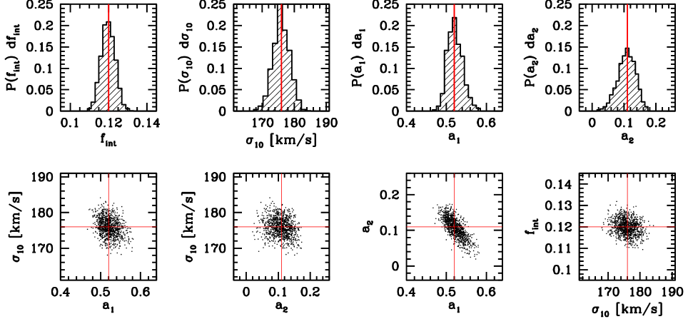
Figure 5: The upper panels plot distributions of $f_{\rm int}$, $\sigma_{10}$, $a_{1}$, and $a_{2}$ (as indicated) obtained from 1000 Monte-Carlo simulations. These are used to estimate errors on these parameters obtained from fitting the distribution of $(\Delta V,L_{\rm host})$ in the MGRS (see text). Thick, vertical lines indicate the input values. The lower panels show two-dimensional scatter plots of these parameters. Horizontal and vertical lines again indicate the input values.

With SC 1 the satellite kinematics can only be measured accurately over about a factor 5 in luminosity (cf. Brainerd & Specian 2003). Therefore, when fitting $\sigma_{\rm sat}(L_{\rm host})$ using the maximum likelihood method we keep $a_{2}$ fixed at zero, such that eq. (28) reduces to a simple power-law. As can be seen, the maximum likelihood method and the discrete Gaussian-plus-constant fits yield satellite velocity dispersions in good agreement with each other. Because $f_{h}$ and $f_{s}$ are not equal to unity with SC 1, it is difficult to compute expectation values for $\sigma_{\rm sat}(L_{\rm host})$ based on the CLF. In order to assess the impact of interlopers and non-central hosts we therefore compute the velocity dispersion of the true satellite galaxies directly from the MGRS: open circles in the upper-left panel of Fig. 4 correspond to $\sqrt{{1\over N}\sum_{i=1}^{N}(\Delta V_{i})^{2}-120^{2}}$ where the summation is over all true satellites (excluding interlopers and satellites around non-central hosts). The best-fit $\sigma_{\rm sat}(L)$, both from the maximum likelihood method as well as from the discrete Gaussian-plus-constant fits, are in good agreement with these true values, indicating that the incomplete correction for interlopers does not significantly influence the satellite kinematics.

In the case of SC 2, the luminosity range over which accurate measurements of $\sigma_{\rm sat}(L)$ can be obtained has increased to almost one and a half orders of magnitude. The $\sigma_{\rm sat}(L)$ is in reasonable agreement with the expectation values computed using eq. (21) with $R_{p}=r_{\rm vir}$ (thick solid line), except for the lowest luminosity bins. This is due to the large fraction of (excess) interlopers and to the presence of satellite galaxies around non-central hosts. Especially the latter can cause a significant overestimate of the true $\sigma_{\rm sat}(L)$. Nevertheless, despite an interloper-fraction of 39 percent, SC 2 allows one to recover the expected $\sigma_{\rm sat}(L)$ with reasonable accuracy.

The results for SC 3 are even more promising. Because of the large number of faint host galaxies, $\sigma_{\rm sat}(L_{\rm host})$ can be measured over two and a half orders of magnitude down to $\sim 4\times 10^{8}h^{-2}\>{\rm L_{\odot}}$. The $\sigma_{\rm sat}$ obtained are in good agreement with the expectation values (solid line, computed using eq. (21) with $R_{p}=0.375r_{\rm vir}$) , even in the regime where $\sigma_{\rm sat}<120\>{\rm km}\,{\rm s}^{-1}$. The dashed line indicates the best-fit $\sigma_{\rm sat}(L_{\rm host})$ obtained from the maximum-likelihood method, the corresponding parameters of which are listed in Table 2.

Fitting eq. (28) directly to the expected $\sigma_{\rm sat}(L_{\rm host})$ (solid line in the lower right-hand panel of Fig. 4) yields as best-fit parameters: $\sigma_{10}=178\>{\rm km}\,{\rm s}^{-1}$, $a_{1}=0.58$, and $a_{2}=0.10$. Thus, the expectation is somewhat steeper than the actual best-fit relation (for which $a_{1}=0.52$). In order to address the significance of this difference we proceed as follows: we construct Monte-Carlo samples based on $\sigma_{10}=176\>{\rm km}\,{\rm s}^{-1}$, $a_{1}=0.52$, $a_{2}=0.11$, and $f_{\rm int}=0.12$, corresponding to the best-fit values obtained for the MGRS. For each of the 16841 satellite galaxies in the MGRS we randomly draw a $\Delta V$ from equation (29), using $f_{\rm int}$ and $\sigma_{\rm sat}(L_{\rm host})$ given by eq. (28). To this $\Delta V$ we add a Gaussian deviate with standard deviation of $120\>{\rm km}\,{\rm s}^{-1}$ to mimic the velocity errors. This yields a sample of $(\Delta V,L_{\rm host}$) with the same distributions of $L_{\rm host}$ and $N_{\rm sat}$ as for the MGRS. Next we apply the maximum likelihood method and find the best-fit values of $(\sigma_{10},a_{1},a_{2},f_{\rm int})$. The distributions of these best-fit values, obtained from 1000 of these Monte-Carlo samples, are shown in Fig. 5. Clearly, the maximum-likelihood method accurately recovers the input values of $\sigma_{10}$, $a_{1}$, $a_{2}$, and $f_{\rm int}$ (indicated by vertical and horizontal lines) with $1\sigma$ errorbars of $3\>{\rm km}\,{\rm s}^{-1}$, $0.02$, $0.04$ and $0.005$, respectively (and with the errors on $a_{1}$ and $a_{2}$ somewhat correlated). Given these random errors, the difference between the dashed and solid lines is marginally significant, reflecting the effect of interlopers and (mainly) satellites around non-central hosts. Nevertheless, the difference is sufficiently small, that we conclude that it is possible to use large, flux limited redshift surveys to obtain accurate estimates of the velocity dispersion of satellite galaxies in haloes that span a wide range of masses. However, keep in mind that these are biased with respect to the host-averaged means.

4 Results for the 2dFGRS

We now focus on real data. We use the final, public data release from the 2dFGRS, restricting ourselves only to galaxies with redshifts $0.01\leq z\leq 0.15$ in the North Galactic Pole (NGP) and South Galactic Pole (SGP) subsamples with a redshift quality parameter $q\geq 3$. This leaves a grand total of $146735$ galaxies with a typical rms redshift error of $85\>{\rm km}\,{\rm s}^{-1}$ (Colless et al. 2001). Absolute magnitudes for galaxies in the 2dFGRS are computed using the K-corrections of Madgwick et al. (2002).

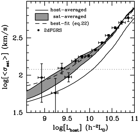
Figure 6: Solid dots with errorbars indicate the best-fit $\sigma_{\rm sat}(L_{\rm host})$ obtained from the 2dFGRS data. The dashed line indicates the corresponding best-fit function of the form (28) obtained using the maximum likelihood method described in the text. The gray area indicates the expectation values obtained using the CLF, where the upper and lower boundary correspond to ‘random’ and ‘constrained’ luminosity sampling, respectively. The solid line indicates the corresponding host-averaged mean $\sigma_{\rm sat}(L_{\rm host})$ and is shown for comparison.

4.1 Satellite Kinematics

Applying our adaptive selection criterion (SC 3) to the 2dFGRS yields 8132 host galaxies and 12569 satellite galaxies. The first thing to notice is that these numbers are quite a bit smaller than for the MGRS. In order to check whether this is consistent with cosmic variance, we constructed four independent MGRSs, using different $L_{100}$ and $L_{300}$ simulation boxes. Applying SC 3 to each of these MGRSs yields $N_{\rm host}=10600\pm 300$ and $N_{\rm sat}=16300\pm 550$. Clearly, the deficit of host and satellite galaxies in the 2dFGRS compared to our MGRS is very significant. We address the abundances of host and satellite galaxies in much more detail in a forthcoming paper (van den Bosch et al. , in preparation). For the moment, however, we ignore this discrepancy and focus on the kinematics only.

Results are shown in Fig. 6. Solid dots with errorbars indicate the $\sigma_{\rm sat}(L_{\rm host})$ obtained by fitting a Gaussian-plus-constant. The thick dashed line indicates the best-fit $\sigma_{\rm sat}(L_{\rm host})$ obtained using the maximum likelihood method (with the best-fit parameters listed in Table 2). The gray area indicates the expectation values obtained from our CLF where the upper and lower boundaries correspond to ‘random’ and ‘constrained’ luminosity sampling, respectively. Clearly, the satellite kinematics obtained from the 2dFGRS are in excellent agreement with these predictions. For comparison, the solid line indicates the expectation value obtained using host-averaging (see discussion in Section 3.2). As already discussed, the flux limit of the 2dFGRS and the satellite-averaging results in a significant bias of the measured $\sigma_{\rm sat}(L_{\rm host})$ compared to this host-averaged mean.

The expectation values (gray area) are computed assuming no spatial bias between satellite galaxies and the dark matter mass distribution. As we have shown in Section 3.2.1, the effect of spatial bias, and the resulting velocity bias, is small compared to the uncertainties resulting from the luminosity sampling. In other words, deviations of the true $n_{\rm sat}(r)$ from the NFW distribution assumed here will not significantly affect our main conclusion that the satellite kinematics of the 2dFGRS are in excellent agreement with predictions based on our CLF.

5 Summary

Previous attempts to measure the kinematics of satellite galaxies have mainly focussed on isolated spiral galaxies. Using detailed mock galaxy redshift surveys we investigated to what extent a similar analysis can be extended to include a much wider variety of systems, from isolated galaxies to massive groups and clusters. Our method is based on the assumption that satellite galaxies are an isotropic, steady-state tracer population orbiting within spherical NFW dark matter haloes, and that the brightest galaxy in each halo resides at rest at the halo centre. These assumptions are, at least partially, supported by both observations of cluster galaxies (i.e., van der Marel et al. 2000) and by numerical simulations of dark matter subhaloes (see Diemand et al. 2004 and references therein). Although there are most definitely systems in which one or more of these assumptions break down, we hypothesized that with sufficiently large samples of host-satellite pairs the occasional ‘perturbed’, non-relaxed, system will not significantly influence the results. In addition, we have shown that the assumption of orbital isotropy only influences the velocity dispersion of satellite galaxies at the few percent level.

We used the conditional luminosity function (CLF) formalism to make predictions of the observed velocity dispersion of satellite galaxies around host galaxies of different luminosity. We showed that the satellite weighting, which occurs naturally when stacking many host-satellite pairs to increase signal-to-noise, introduces a bias towards higher $\sigma_{\rm sat}(L_{\rm host})$ compared to the true, host-averaged mean. A further bias, in the same direction, is introduced when using flux-limited, rather than volume-limited surveys. Finally, we demonstrated that most of the uncertainty in interpreting the measured $\sigma_{\rm sat}(L_{\rm host})$ owes to the unknown second moment of the conditional probability distribution $P(M|L_{\rm host})$: typically a larger second moment yields higher expectation values. The CLF formalism is the ideal tool to properly take all these various biases into account.

An important, additional problem with the interpretation of satellite kinematics is how to deal with the presence of interlopers (i.e., galaxies selected as satellites but which are not physically associated with the halo of the host galaxy) and non-central hosts (i.e., galaxies that are selected as host galaxies, but which are not the central, brightest galaxy in their own halo). The abundances of interlopers and non-central hosts depend strongly on the selection criteria. Using MGRSs, constructed from the CLF, we investigated different selection criteria for hosts and satellites. The first one is identical to the criteria used by McKay et al. (2002) and Brainerd & Specian (2003) in their analyses of satellite kinematics in the SDSS and 2dFGRS, respectively. Applied to our MGRS it yields only 3876 satellites, which only allows an analysis of satellite kinematics around host galaxies that span a factor 5 in luminosity. Although the fraction of non-central hosts is, with one percent, negligible, the fraction of interlopers is 27 percent. More importantly, the interloper fraction increases strongly with decreasing host-luminosity, reaching values as high as 60 percent around the faintest host galaxies. Contrary to what has been assumed in the past (e.g., McKay et al. 2002; Brainerd & Specian 2003), the velocity distribution of interlopers is strongly peaked towards $\Delta V=0$, similar to the distribution of true satellite galaxies. This makes a detailed correction for interlopers extremely difficult. In fact, the method used thus far, based on the assumption of a uniform $P(\Delta V)$, typically underpredicts the true interloper fraction by $\sim 50$ percent.

We therefore devised an iterative, adaptive selection criterion that yields large numbers of hosts and satellites with as few interlopers and non-central hosts as possible. Applying these criteria to our MGRS yields 16750 satellites around 10483 hosts. In addition, the interloper fraction is only 14 percent and, more importantly, does not vary significantly with host luminosity. Because of the much larger numbers involved, and the reduced fraction of interlopers, satellite kinematics can be analyzed over two and a half orders of magnitude in $L_{\rm host}$. The resulting $\sigma_{\rm sat}(L_{\rm host})$ is found to be in good agreement with the expectation values, indicating that the interlopers and non-central hosts do not significantly distort the measurements.

Finally, we applied our adaptive selection criteria to the 2dFGRS. The resulting satellite kinematics are in excellent agreement with predictions based on the CLF formalism, once the various biases discussed above are taken into account. We therefore conclude that the observed kinematics of satellite galaxies provide virtually independent, dynamical confirmation of the average mass-to-light ratios inferred by Yang et al. (2003a) and van den Bosch et al. (2003a) from a purely statistical method based on the abundances and clustering properties of galaxies in the 2dFGRS.

Appendix A The conditional luminosity function

The construction of our mock galaxy redshift surveys uses the conditional luminosity function (CLF) to indicate how many galaxies of given luminosity occupy a halo of given mass. The CLF formalism was introduced by Yang et al. (2003a) and van den Bosch et al. (2003a), and we refer the reader to these papers for more details. Here we briefly summarize the main ingredients and we present the parameterization used.

The CLF is parameterized by a Schechter function:

$$\Phi(L|M){\rm d}L={\tilde{\Phi}^{*}\over\tilde{L}^{*}}\,\left({L\over\tilde{L}^{*}}\right)^{\tilde{\alpha}}\,\,{\rm exp}(-L/\tilde{L}^{*})\,{\rm d}L,$$ (31)

where $\tilde{L}^{*}=\tilde{L}^{*}(M)$, $\tilde{\alpha}=\tilde{\alpha}(M)$ and $\tilde{\Phi}^{*}=\tilde{\Phi}^{*}(M)$ are all functions of halo mass $M$. We write the average, total mass-to-light ratio of a halo of mass $M$ as

$$\left\langle{M\over L}\right\rangle(M)={1\over 2}\,\left({M\over L}\right)_{0}\left[\left({M\over M_{1}}\right)^{-\gamma_{1}}+\left({M\over M_{1}}\right)^{\gamma_{2}}\right],$$ (32)

This parameterization has four free parameters: a characteristic mass $M_{1}$, for which the mass-to-light ratio is equal to $(M/L)_{0}$, and two slopes, $\gamma_{1}$ and $\gamma_{2}$, that specify the behavior of $\langle M/L\rangle$ at the low and high mass ends, respectively. Motivated by observations (Bahcall, Lubin & Norman 1995; Bahcall et al. 2000; Sanderson & Ponman 2003; Eke et al. 2004), which indicate a flattening of $\langle M/L\rangle(M)$ on the scale of galaxy clusters, we set $\langle M/L\rangle(M)=(M/L)_{\rm cl}$ for haloes with $M\geq 10^{14}h^{-1}\>{\rm M_{\odot}}$. With $(M/L)_{\rm cl}$ specified, the value for $\gamma_{2}$ derives from requiring continuity in $\langle M/L\rangle(M)$ across $M=10^{14}h^{-1}\>{\rm M_{\odot}}$.

A similar parameterization is used for the characteristic luminosity $\tilde{L}^{*}(M)$:

$${M\over\tilde{L}^{*}(M)}={1\over 2}\,\left({M\over L}\right)_{0}\,f(\tilde{\alpha})\,\left[\left({M\over M_{1}}\right)^{-\gamma_{1}}+\left({M\over M_{2}}\right)^{\gamma_{3}}\right],$$ (33)

with

$$f(\tilde{\alpha})={\Gamma(\tilde{\alpha}+2)\over\Gamma(\tilde{\alpha}+1,1)}.$$ (34)

Here $\Gamma(x)$ is the Gamma function and $\Gamma(a,x)$ the incomplete Gamma function. This parameterization has two additional free parameters: a characteristic mass $M_{2}$ and a power-law slope $\gamma_{3}$. For $\tilde{\alpha}(M)$ we adopt a simple linear function of $\log(M)$,

$$\tilde{\alpha}(M)=\alpha_{15}+\eta\,\log(M_{15}),$$ (35)

with $M_{15}$ the halo mass in units of $10^{15}\>h^{-1}\rm M_{\odot}$, $\alpha_{15}=\tilde{\alpha}(M_{15}=1)$, and $\eta$ describes the change of the faint-end slope $\tilde{\alpha}$ with halo mass. Finally, we introduce the mass scale $M_{\rm min}$ below which we set the CLF to zero; i.e., we assume that no stars form inside haloes with $M<M_{\rm min}$. Motivated by reionization considerations (see Yang et al. 2003a for details) we adopt $M_{\rm min}=10^{9}h^{-1}\>{\rm M_{\odot}}$ throughout.

In this paper we use a CLF with the following parameters: $M_{1}=10^{11.12}h^{-1}\>{\rm M_{\odot}}$, $M_{2}=10^{11.71}h^{-1}\>{\rm M_{\odot}}$, $(M/L)_{0}=85h\>({\rm M}/{\rm L})_{\odot}$, $\gamma_{1}=1.55$, $\gamma_{2}=0.46$, $\gamma_{3}=0.69$, $\eta=-0.29$ and $\alpha_{15}=-0.99$. This model is different from those listed in van den Bosch et al. (2003a) as it yields a higher, average mass-to-light ratio on the scale of clusters. As shown in Yang et al. (2003b), this is in better agreement with the observed pairwise peculiar velocity dispersions of 2dFGRS galaxies (see also van den Bosch, Mo & Yang 2003b). However, none of the results presented in this paper are sensitive to our choice of the CLF. We verified that MGRSs based on either of the CLFs listed in van den Bosch et al. (2003a) yield virtually identical results to those presented here.

Appendix B Probability distribution of luminosity of brightest galaxy in a dark matter halo.

Define $L_{c}$ as the luminosity of the brightest galaxy in a halo of mass $M$. It is convenient to write the conditional probability distribution $P(L_{c}|M){\rm d}L_{c}$ in terms of the conditional luminosity function $\Phi(L_{c}|M){\rm d}L_{c}$ and a new function $f(L_{c},M)$ which depends on how galaxy luminosities are drawn from the CLF:

$$P(L_{c}|M){\rm d}L_{c}=\Phi(L_{c}|M)\,f(L_{c},M)\,{\rm d}L_{c}$$ (36)

In the case of ‘constrained’ drawing, $L_{c}$ has an expectation value given by eq. (5), and it is straightforward to show that

$$f(L_{c},M)=\left\{\begin{array}[]{ll}1&\mbox{if $L_{c}\geq L_{1}(M)$}\\ 0&\mbox{if $L_{c}<L_{1}(M)$}\end{array}\right.$$ (37)

with $L_{1}(M)$ as defined by eq. (4). Note that in the MGRS used in this paper the luminosity of the brightest galaxy in each halo is always drawn constrained. Therefore, when computing expectation values for $\sigma_{\rm sat}(L_{\rm host})$ in the MGRS, we use $P(L_{c}|M)$ with $f(L_{c},M)$ given by eq. (37).

In the case of ‘random’ drawing, the situation is more complicated. The probability that a galaxy drawn at random from the CLF has a luminosity less than $L_{c}$ is given by

$$P(<L_{c}|M)=1-{1\over\langle N\rangle_{M}}\int_{L_{c}}^{\infty}\Phi(L|M){\rm d}L$$ (38)

with $\langle N\rangle_{M}$ the mean number of galaxies in a halo of mass $M$ given by eq. (1). In a halo with $N$ galaxies, the probability that the brightest galaxy has $L<L_{c}$ is simply $[P(<L_{c}|M)]^{N}$. Differentiating with respect to $L_{c}$ yields the probability $P_{N}(L_{c}|M){\rm d}L_{c}$ that after $N$ drawings the brightest galaxy has a luminosity in the range $L_{c}\pm L_{c}/2$. The full probability $P(L_{c}|M){\rm d}L_{c}$ follows from summing $P_{N}(L_{c}|M){\rm d}L_{c}$ over $N$, properly weighted by the probability $P(N|M)$ that a halo of mass $M$ contains $N$ galaxies. This yields

$$f(L_{c},M)={1\over\langle N\rangle_{M}}\sum_{N=1}^{\infty}N\,P(N|M)\,\left[P(<L_{c}|M)\right]^{N-1}$$ (39)

If $\langle N\rangle_{M}\leq 1$ then

$$P(N|M)=\left\{\begin{array}[]{ll}1-\langle N\rangle_{M}&\mbox{if $N=0$}\\ \langle N\rangle_{M}&\mbox{if $N=1$}\end{array}\right.$$ (40)

(see Section 2.2), so that $f(L_{c},M)=1$. For $\langle N\rangle_{M}>1$ we have that

$$P(N|M)={(\langle N\rangle-1)^{N-1}\over(N-1)!}\,{\rm exp}(1-\langle N\rangle_{M})$$ (41)

(see Section 2.2). Substituting (41) in (39) and using that

$$\sum_{k=0}^{\infty}{x^{k}\over k!}(k+1)=(1+x)\,{\rm exp}(x)$$ (42)

(see eq. [1.212] in Gradshteyn & Ryzhik, 1980) yields

$$f(L_{c},M)=\left(1-{\zeta\over\langle N\rangle_{M}}\right)\,{\rm exp}(-\zeta)$$ (43)

with

$$\zeta={\langle N\rangle_{M}-1\over\langle N\rangle_{M}}\,\int_{L_{c}}^{\infty}\Phi(L|M){\rm d}L$$ (44)

References

- [] Bahcall N.A., Lubin L., Dorman V., 1995, ApJ, 447, L81
- [] Bahcall N.A., Cen R., Davé R., Ostriker J.P., Yu Q., 2000, ApJ, 541, 1
- [] Benson A.J., Cole S., Frenk C.S., Baugh C.M., Lacey C.G., 2000, MNRAS, 311, 793
- [] Berlind A.A., Weinberg D.H., 2002, ApJ, 575, 587
- [] Berlind A.A., et. al., 2003, ApJ, 593, 1
- [] Binney J.J., Tremaine S.D., 1987, Galactic Dynamics (Princeton: Princeton Univ. Press)
- [] Brainerd T.G., Specian M.A., 2003, ApJ, 593, L7
- [] Carlberg R.G., Yee H.K.C., Ellingson E., Abraham R., Gravel P., Morris S., Pritchet C.J., 1996, ApJ, 462, 32
- [] Carlberg R.G., et al., 1997a, ApJ, 485, L13
- [] Carlberg R.G., Yee H.K.C., Ellingson E., 1997b, ApJ, 478, 462
- [] Colin P., Klypin A., Kravtsov A.V., Khokhlov M., 1999, ApJ, 532, 32
- [] Colless M., The 2dFGRS team, 2001, MNRAS, 328, 1039
- [] Davis M., Efstathiou G., Frenk C.S., White S.D.M., 1985, ApJ, 292, 371
- [] De Lucia G., Kauffmann G., Springel V., White S.D.M., Lanzoni B., Stoehr F., Tormen G., Yoshida N., 2004, MNRAS, 348, 333
- [] Diemand J., Moore B., Stadel J., 2004, preprint (astro-ph/0402160)
- [] Eke V.R., Navarro J.F., Steinmetz M., 2001, ApJ, 554, 114
- [] Eke V.R., The 2dFGRS team, 2004, preprint (astro-ph/0402566)
- [] Erickson L.K., Gottesman S.T., Hunter J.H., 1987, Nature, 325 779
- [] Evans N.W., Wilkinson M.I., 2000, MNRAS, 316, 929
- [] Evans N.W., Wilkinson M.I., Guhathakurta P., Grebel E.K., Vogt S.S., 2000, ApJ, 540, L9
- [] Ghigna S., Moore B., Governato F., Lake G., Quinn T., Stadel J., 1998, MNRAS, 300, 146
- [] Gradshteyn I.S., Ryzhik I.M., 1980, Table of Integrals, Series, and Products. Academic Press, New York
- [] Jing Y.P., 2002, MNRAS, 335, L89
- [] Jing Y.P., Suto, Y., 2002, ApJ, 574, 538
- [] Klypin A., Gottlöber S., Kravtsov A.V., Khokhlov A.M., 1999, ApJ, 516, 530
- [] Kravtsov A.V., Berlind A.A., Wechsler R.H., Klypin A.A., Gottlöber S., Allgood B., Primack J.R., 2003, preprint (astro-ph/0308519)
- [] Lin D.N.C., Jones B.F., Klemola A.R., 1995, ApJ, 439, 652
- [] Lin Y.-T., Mohr J.J., Stanford S.A., 2004, preprint (astro-ph/0402308)
- [] Little B., Tremaine S., 1987, 320, 493
- [] Maddox S.J., Efstathiou G., Sutherland W.J., Loveday L., 1990, MNRAS, 243, 692
- [] Madgwick D.S., The 2dFGRS team, 2002, MNRAS, 333, 133
- [] McKay T.A. et al., 2002, ApJ, 571, L85
- [] Moore B., Governato G., Quinn T., Stadel J., Lake G., 1998, ApJ, 499, L5
- [] Navarro J.F., Frenk C.S., White S.D.M., 1997, ApJ, 490, 493
- [] Norberg P., The 2dFGRS team, 2002a, MNRAS, 332, 827
- [] Norberg P., The 2dFGRS team, 2002b, MNRAS, 336, 907
- [] Okamoto T., Habe A., 1999, ApJ, 516, 591
- [] Prada F., et al., 2003, ApJ, 598, 260
- [] Rhines K., Geller M.J., Diaferio A., Kurtz M.J., Jarrett T.H., 2004, preprint (astro-ph/0402242)
- [] Sanderson A.J.R., Ponman T.J., 2003, MNRAS, 345, 1241
- [] Scoccimarro R., Sheth R.K., Hui L., Jain B., 2001, ApJ, 546, 20
- [] Seljak U.,2000, MNRAS, 318, 203
- [] Sheth R.K., Mo H.J., Tormen G., 2001a, MNRAS, 323, 1
- [] Sheth R.K., Tormen, G., 2002, MNRAS, 329, 61
- [] Springel V., White S.D.M., Tormen G., Kauffmann G., 2001, MNRAS, 328, 726
- [] Vale A., Ostriker J.P., 2004, preprint (astro-ph/0402500)
- [] van den Bosch F.C., Yang X., Mo H.J., 2003a, MNRAS, 340, 771
- [] van den Bosch F.C., Mo H.J., Yang X., 2003b, MNRAS, 345, 923
- [] van der Marel R.P., Magorrian J., Carlberg R.G., Yee H.K.C., Ellingson E., 2000, AJ, 119, 2038
- [] Yang X., Mo H.J., van den Bosch F.C., 2003a, MNRAS, 339, 1057
- [] Yang X., Mo H.J., Jing Y.P., van den Bosch F.C., Chu Y., 2003b, MNRAS, in press (astro-ph/0303524)
- [] York D., et al., 2000, AJ, 120, 1579
- [] Zaritsky D., Smith R., Frenk C.S., White S.D.M., 1993, ApJ, 405, 464
- [] Zaritsky D., White S.D.M., 1994, ApJ, 435, 599
- [] Zaritsky D., Smith R., Frenk C.S., White S.D.M., 1997, ApJ, 478, 39
- [] Zwicky F., 1933, Helv. Phys. Acta, 6, 110
- [] Zwicky F., 1937, ApJ, 86, 217