Hydrodynamic stability of rotationally supported flows: Linear and nonlinear 2D shearing box results

We present here both analytical and numerical results of hydrodynamic stability investigations of rotationally supported circumstellar flows using the shearing box formalism. Asymptotic scaling arguments justifying the shearing box approximation are systematically derived, showing that there exist two limits which we call small shearing box (SSB) and large shearing box (LSB). The physical meaning of these two limits and their relationship to model equations implemented by previous investigators are discussed briefly. Two dimensional (2D) dynamics of the SSB are explored and shown to contain transiently growing (TG) linear modes, whose nature is first discussed within the context of linear theory. The fully nonlinear regime in 2D is investigated numerically for very high Reynolds (Re) numbers. Solutions exhibiting long-term dynamical activity are found and manifest episodic but recurrent TG behavior and these are associated with the formation and long-term survival of coherent vortices. The life-time of this spatio-temporal complexity depends on the Re number and the strength and nature of the initial disturbance. The dynamical activity in finite Re solutions ultimately decays with a characteristic time increasing with Re. However, for large enough Re and appropriate initial perturbation, a large number of TG episodes recur before any viscous decay begins to clearly manifest itself. In cases where Re = $\infty$ nominally (i.e. any dissipation resulting only from numerical truncation errors), the dynamical activity persists for the entire duration of the simulation (hundreds of box orbits). Because the SSB approximation used here is equivalent to a 2D incompressible flow, the dynamics can not depend on the Coriolis force. Therefore, three dimensional (3D) simulations are needed in order to decide if this force indeed suppresses nonlinear hydrodynamical instability in rotationally supported disks in the shearing box approximation, and if recurrent TG behavior can still persist in three dimensions as well - possibly giving rise to a subcritical transition to long-term spatio-temporal complexity.

1 Introduction

Accretion of matter, endowed with a significant amount of angular momentum, onto relatively compact objects, is thought to occur in a variety of important astrophysical systems, including close binary stars, young stellar objects and active galactic nuclei. If the accreting matter is able to cool efficiently enough, the resulting configuration of the flow is a vertically thin, almost-Keplerian (that is, essentially rotationally supported), accretion disk. The accretion process (transport of mass inward) can occur only if some dissipative mechanism is present, giving rise to transport of angular momentum outward. Since the microscopic viscosity of the fluids in question is very small, and thus the Re numbers of such flows are literally astronomical, anomalous transport of some kind must be invoked to account for the time scales and magnitude of the energy output of the accreting sources. The pioneering works of Shakura & Sunyaev (1973) and Lynden-Bell & Pringle (1972) suggested that the needed anomalous transport can be naturally achieved if the accretion flow is turbulent and, moreover, proposed to circumvent the complexities and our lack of understanding of turbulence by introducing the now famous $\alpha$ model of accretion disks (in the language of turbulence modeling it is ”a zero-equation, one-parameter model”). This simple idea has been extremely fruitful, giving rise to a large number of successful interpretations of observational results (see e.g. Pringle 1981 and Frank, King & Raine 2002 for reviews).

The theoretical question of the physical origin of accretion disk turbulence has however remained essentially unanswered until Balbus & Hawley (1991) discovered that weak magnetic fields destabilize differential Keplerian rotation, i.e. the magneto-rotational instability (Velikhov 1959, Chandrasekhar 1960), hereafter MRI, can operate in rotationally supported magnetized accretion disks, rendering them linearly unstable. This instability was subsequently recognized as the source of accretion disk magneto-hydrodynamic (MHD) turbulence, giving rise to the needed angular momentum transport and also to dynamo action (Hawley, Gammie & Balbus 1995; Brandenburg et al. 1995). For a recent review of this topic see Balbus (2003). The discovery by Balbus & Hawley is very important and significant because it demonstrates the existence of linear instability in accretion disk models with angular velocity profiles that are otherwise stable according to the Rayleigh criterion. Although some ideas have been put forward in this context, e.g. the possibility of an instability resulting from the angular velocity being nonconstant on cylinders (Knobloch & Spruit knobloch (1986), Kluźniak & Kita 1997, Regev & Gitelman 2002, Urpin 2003) or more general baroclinic instabilities (Klahr & Bodenheimer 2003), no hydrodynamic instability of any kind has ever been explicitly shown to exist. In the absence of a known linear hydrodynamic instability, the turbulent viscosity needed for angular momentum transport in accretion disks has acquired in the community a somewhat ”mysterious” character, similar to other ignorance-driven concepts in the history of astrophysics (and physics). Thus the MRI has been generally accepted with considerable enthusiasm and, as it often happens in cases where a successful idea is advanced, raised to the level of an exclusive paradigm. Moreover, the very possibility of the occurrence of hydrodynamic turbulence (resulting from linear or even nonlinear hydrodynamical instabilities) has been questioned by Balbus, Hawley & Stone (1996) (see also the detailed study of Hawley, Balbus & Winters 1999), hereafter BHSW, on the basis of the results of fully nonlinear finite-difference numerical simulations in the 3D shearing box approximation (see below).

The extreme displeasure felt by most astrophysicists with the absence of linear hydrodynamical disk instabilities, and their reluctance in accepting that disks may still be hydrodynamically turbulent, seems to be detached from what has been known for the past century on hydrodynamical stability of shear flows. It is well known (see e.g. Joseph 1972, Drazin & Reid 1983) that the linear stability properties of essentially all the canonical shear flows, rotating or not, do not reproduce well their laboratory behavior. In almost all such flows transition to turbulence is subcritical, that is, it occurs at Reynolds numbers (Re) that are significantly lower (and also dependent on the perturbation strength) than the critical values for linear instability ${\rm Re_{c}}$. In some instances, like the pipe Poiseulle, plane Couette or Taylor-Couette (in the narrow gap limit) flows, this problem is particularly acute as linear analysis of perturbations on these basic flow profiles predicts stability (even decay) of infinitesimal perturbations, that is, formally ${\rm Re_{c}}=\infty$. Laboratory experiments demonstrate, however, full-on transition to turbulence via some instability mechanism that is neither fully understood nor even uniquely identified. Thus various ideas in this context are generally referred to as transition scenarios (see below).

On the theoretical side, it has been known since the work of Orr (1907) that even though a basic shear flow may be linearly stable, some perturbations (i.e. initial conditions) may exhibit significant transient growth (TG) within the linear regime, before ultimately decaying. This fact prompted a number of researchers to examine the possibility of subcritical transition to turbulence, with the linearly stable flow finding a way to bypass the usual (i.e. via linear instability) route to turbulence. We are unable to mention here all the contributions on this subject (in particular, those published before the early 1990s) and refer the interested reader to one of the reviews cited below, but only note that an application of TG to an astrophysical problem has already been implemented by Goldreich & Lynden-Bell (1965).

A significant step forward in the advancement of the bypass transistion idea has been made in the early 1990s. It came with the clarification that TG, and thus the possibility of a bypass transition, is the result of the linearized system’s operator properties (Butler & Farrell 1992, Reddy & Henningson 1993). The essence of this idea lies in the observation that linear stability analysis of shear flows gives rise to a nonnormal operator(i.e. an operator which does not commute with its adjoint), that is, one whose eigenfunctions are not necessarily orthogonal. This rather elementary mathematical fact may have profound consequences for hydrodynamic stability, because it explains how TG may naturally occur in linearly stable basic shear flows (see e.g. Trefethen et al. 1993). This approach is frequently referred to as nonmodal because the linear stability analysis required to find TG cannot proceed via the usual modal analysis, involving a boundary value problem and must consist of the examination of the original initial value problem. If this TG is strong enough then nonlinear interactions may come into play. This then could further lead to some kind of ”nonlinear instability” creating a sustained complex dynamical state in which TG events persistently recur and resulting in a situation resembling turbulence. We shall refer to this phenomenon as recurrent transient growth (RTG). The recent review by Grossmann (2000) contains an excellent account of these ideas. We refer the reader also to the comprehensive modern book on shear flow instabilities (Schmid & Henningson 2001) and relevant references within, where a detailed account (a full chapter) on the different ideas on transition to turbulence in shear flows are detailed.

The above developments recently have been brought to the attention of the astrophysical community by Ioannaou & Kakouris (2001) and Chagelishvili et al. (2003) in the context of accretion disks. These two studies are quite different in their approach - the former examines global behavior of disturbances in an accretion disk and the latter is a local analysis in the framework of the shearing box (SB), also sometimes called the shearing sheet, approximation - but they both utilize the basic idea mentioned above. It appears that although these works have not explicitly demonstrated that a turbulent state of an accretion disk actually arises by purely hydrodynamical processes, they have convincingly suggested that such a process is feasible. The purpose of this (and subsequent) work is to carry this idea further and examine in detail the nonlinear regime in various limits.

There is little doubt that whenever MRI occurs in a disk it leads to a turbulent flow with enhanced angular momentum transport outward. However, BHSW (see also Balbus 2003) put forth the claim that no purely hydrodynamical process can destabilize a Keplerian accretion disk, at least within the SB approximation. This is based on fully nonlinear simulations (performed by BHSW) in which no (nonlinear) hydrodynamic instability was shown to manifest itself as long as the angular velocity profile was linearly stable according to the Rayleigh criterion. Furthermore, the same simulations of BHSW also show that the total kinetic energy of plane Couette flow and rotating flows which are unstable according to the Rayleigh criterion, grow essentially monotonically (after a short transient). By contrast, in Rayleigh-stable rotation profiles the kinetic energy was observed to decay over the duration of the runs (typically 5-10 box orbit times).

Since in the SB approximation it is the Coriolis term that actually distinguishes between simple plane Couette flow and the flow within a small segment of a rotating disk (see below), it is only natural that this force has been identified by BHSW as the stabilizing agent.

These numerical results certainly constitute a serious challenge to the possibility of hydrodynamic turbulence in rotationally supported disks. On the other hand, we can state at least five observations which suggest that this matter is far from being settled.

1. In some astrophysical systems containing such disks the conditions are such that MRI driven MHD turbulence is probably impossible. For example, accretion disks in dwarf novae during quiescence (Menou 2000) and around forming stars (Blaes & Balbus 1994, Sano et al. 2000) seem to be too resistive to support MHD turbulence.

2. Recent laboratory Couette-Taylor experiments in the narrow gap limit, with linearly stable rotational angular velocity profiles (like in Keplerian disks) indicate the development of turbulence in such flows (Richard 2001, see also Richard & Zahn 1999).

3. In a recent thoughtful examination of the problem, Longaretti (2002) proposes that the above conclusion reached by BHSW, about the role of the Coriolis force in suppressing the subcritical transition (observed in non-rotating plane Couette flows in the lab and in BHSW simulations), may be premature. He speculates that their findings may stem from the inability (of the simulations) to resolve some of the essential dynamics within these rotating flows (see however Balbus 2003).

4. There exist numerical simulations of plane Couette flows, which have revealed the details of what can be called ”subcritical turbulence” in these flows (Schmiegel & Eckhardt, 1997; Eckhardt et al. 1998). These calculations, which are the only ones (as far as we know) of this kind and extend for reasonably long integration times, indicate that above a critical Reynolds number there appears dynamical activity, resulting probably from repeated TG events, brought about by nonlinear interaction and persisting much longer than the viscous decay time, i.e. RTG. This nature of the subcritical bypass transition appears to be very different from a ”usual” supercritical transition to turbulence via linear instability. In particular the outcome critically depends on the initial perturbation, in addition to the Reynolds number. Similar dependence is observed in experiments (see Grossman 2000). It is therefore quite surprising that in BHSW the non-rotating Couette flow (which is linearly stable and hence must have a subcritical transition and thus probably RTG) and the rotating Rayleigh (linearly) unstable flows exhibit a similar perturbation energy growth, at least during the relatively short duration of the BHSW simulations and for a particular choice of the initial perturbation.

5. In relation to the last point, the simulations of BHSW only consider one type of initial conditions to seed their flows and they follow its evolution for, at most, a dozen orbit times. Perturbation spectra are surely myriad and it is possible that conditions leading to a subcritical transition into turbulence may have been overlooked by BHSW.

Thus, it seems that continued study of purely hydrodynamical processes in disks still remains viable and worthwhile (in the words of Balbus, Hawley & Stone 1996) and, in particular, the issue of hydrodynamical stability warrants perhaps a new look.

In this paper we will report on our first effort in this direction. Our goal will be to critically evaluate, using high resolution and long duration (hundreds of box orbit times, that is, Kepler rotational periods at the radius of the box location) numerical experiments in the nonlinear regime, whether the linear TG mechanism is sufficient to induce a bypass transition into a persistently dynamically active state, like the one described in item (4) above. We shall employ spectral methods (wherever possible) for our simulations, as these methods are generally regarded in the fluid-dynamical community as being more accurate and reliable than finite difference schemes. For the time being we shall focus just on the nature of the instability and the possibility of a sustained spatio-temporal complexity. The issue whether in such a state there is an enhanced angular momentum transport outward (as it must be in accretion disks) is an important one (see Cabot 1966, Balbus 2003), but its exploration must await a conclusive result on the instability itself and thus we shall not deal with it in the present work.

This paper is organized in the following way. In Section 2 we examine and discuss the nondimensional SB equations, as appropriate for the case studies here, in which the size of the box is much smaller than the disk’s vertical scale height. This is one of the limits of the SB approximation, whose systematic and general derivation is detailed in Appendix A. Section 3 deals with linear theory and in particular we apply there the concept of sheared coordinates, with whose help the results of Chagelishvili et al. (2003) (the TG of linear modes) can be elegantly recovered. In section 4 we report the results of nonlinear 2D numerical simulation in this limit of the SB approximation. Although it has been recognized that nonmodal TG may give rise to very large amplification in 3D, also 2D perturbations can grow quite significantly (Trefethen et al. 1993). In two-dimensional viscous incompressible flows any dynamical activity must ultimately decay (see section 4.2 below), however for large enough Re numbers we expect the decay times to be very long (since they should behave as $\propto{\rm Re}^{2/3}$, Yecko 2004) so as to allow for the TG episodes to recur many times.

Thus, in this initial study we limit ourselves to 2D and we postpone to subsequent investigations (which are already in progress) 3D simulations of this and the other limit of the SB approximation.

2 The Shearing Box Approximation Equations:

Numerical simulations of rotationally supported flows at very large Reynolds numbers must focus on only very small disk sections if high spatial resolution is imperative. This is clearly the case when one looks for possible instabilities and therefore most such studies have been done within the shearing box (or sheet) approximation. The essence of this approximation is local in approach, that is, the equations are valid in a small region (a Cartesian box) about a typical point in the disk. In such a box, a steady flow consisting of a linear shear velocity profile solves the equations and one can consider it as a basic flow and perturb around it. The equations for the perturbations (linearized or not) are then referred to as the shearing box (SB) approximation equations. Most numerical simulations of Balbus, Hawley and collaborators in the MRI context have been done within this formalism as have the recent studies, mentioned above, on the feasibility of a hydrodynamical instability. Although the SB approximation is not new (Goldreich & Lynden Bell 1965) we have not found in the literature a systematic derivation of this approximation. Thus, in the purpose of resolving the confusion (of the present authors and possibly also others) we give here in Appendix A such a derivation, giving rise to two limits of this approximation.

In the first one, a box whose size is much smaller than the smallest scale height in the disk (usually the one in the vertical direction) is considered, and thus the unperturbed state of linear shear may be considered homogeneous. The perturbations are then incompressible and acoustics are ruled out. Most previously relevant work have been done in this approximation, which we call small shearing box (SSB). For the sake of completeness we repeat here the non-dimensionalized SSB equations derived in Appendix A. In writing the equations below, we have deviated slightly from the notation presented in Appendix A,

$$\nabla\cdot{\bf u} = 0,$$ (1)

$$\partial_{t}u+2Ax\partial_{y}u-2\Omega_{0}v+{\bf u}\cdot\nabla u = -\frac{\partial_{x}p}{1+\rho^{\prime}},$$ (2)

$$\partial_{t}v+2Ax\partial_{y}v+2(\Omega_{0}+A)u+{\bf u}\cdot\nabla v = -\frac{\partial_{y}p}{{1+\rho^{\prime}}},$$ (3)

$$\partial_{t}w+2Ax\partial_{y}w+{\bf u}\cdot\nabla w = -\frac{\partial_{z}p+z\rho^{\prime}}{1+\rho^{\prime}},$$ (4)

$$\partial_{t}\rho^{\prime}+2Ax\partial_{y}\rho^{\prime}+{\bf u}\cdot\nabla\rho^{\prime} = 0,$$ (5)

and the identifications to the terms in Appendix A are: ${\bf u}\equiv{\bf u^{\prime}}$, $u\equiv u^{\prime}_{x},v\equiv u^{\prime}_{u},w\equiv u^{\prime}_{z}$. We also specifically assume that the disk is exactly Keplerian which means that $\Omega_{0}=1$ and $2A=-3/2$. It also means, by (65), that $\partial_{z}P_{b}=-z$ and $\partial_{x}P_{b}=0$. Additionally, even though $\Omega_{0}=1$, we retain this symbol throughout the calculation for the purpose of flagging the Coriolis terms.

In this paper we exclusively use the SSB approximation and assume that the initial density disturbance is everywhere zero, i.e. $\rho^{\prime}(t=0)=0$. From (5) it follows that $\rho^{\prime}=0$ for all subsequent times. Thus, (5) becomes irrelevant and from here on out it shall not be referenced.

The large shearing box (whose size is of the order the disk thickness) equations are also given in Appendix A and they will be treated in our future works.

3 SSB linear theory - a review

For the sake of economy we reintroduce the parameter $q$ (with $\Omega_{0}=1$) as defined by (56) to replace $-2A$ in the linearized expressions of (1-4):

$$\partial_{x}u+\partial_{y}v+\partial_{z}w = 0,$$ (6)

$$(\partial_{t}-qx\partial_{y})u-2\Omega_{0}v = -\partial_{x}p,$$ (7)

$$(\partial_{t}-qx\partial_{y})v+(2\Omega_{0}-q)u = -\partial_{y}p,$$ (8)

$$(\partial_{t}-qx\partial_{y})w = -\partial_{z}p.$$ (9)

Since this flow is exactly Keplerian, $q=3/2$. As a point of reference: for solid body rotation $q=0$, for flows with constant specific angular momentum $q=2$. These linear equations describe simple incompressible flow with a linear shear profile in a rotating frame: that is, linearized rotating plane Couette flow (Nagata, nagata (1986)).

For two-dimensional disturbances (i.e. when $\partial_{z}=0$, $w=0$), the equations governing the linear evolution simplify. With the vertical component of vorticity defined by,

$$\xi\equiv{\partial_{x}v}-\partial_{y}u,$$ (10)

it follows from (7) and (8) that it is conserved along the shear flow,

$$(\partial_{t}-qx\partial_{y})\xi=0.$$ (11)

Because of the incompressibility of the 2D flow, the velocity components may be derived from a stream function, $\psi$, defined by

$$u=-\partial_{y}\psi,\quad v=\partial_{x}\psi,$$ (12)

and related to the vorticity via

$$\xi=\partial_{x}^{2}\psi+\partial_{y}^{2}\psi.$$ (13)

We note also that the equations governing 2D dynamics are insensitive to the background rotation state even though the kinematics are sensitive to it. If the boundary conditions are independent of rotation too (as is the case here), the velocity distribution (that is the dynamics) cannot depend on the Coriolis term. This is a well known property of the governing equations and it is entirely due to the incompressibility of the flow which facilitates the streamfunction-vorticity formulation (see e.g. Batchelor 1967, p. 178). The resulting equation set, even the nonlinear one, becomes mathematically equivalent to the set appropriate to plane Couette flow. The results of all our 2D calculations are based on solving equations (11) and (13) with periodic boundary conditions (in the sheared frame, see below) and thus they do not depend in any way on the Coriolis force.

To avoid any confusion with language, in this work we interchangeably refer to points with constant values of $x$ and varying values of $y$ as being in the streamwise direction and we refer to points with constant values of $y$ and varying values of $x$ as being in the shearwise direction.

Note that for three-dimensional disturbances one can obtain a single decoupled equation for the radial velocity component $u$ after manipulation of (6-9),

$$(\partial_{t}-qx\partial_{y})^{2}(\partial_{x}^{2}+\partial_{y}^{2}+\partial_{z}^{2})u+2\Omega_{0}(2\Omega_{0}-q)\partial_{z}^{2}u=0.$$ (14)

Finally we point out that the same manipulations show that the pressure is related to the radial velocity by

$$\partial_{y}^{2}p+\partial_{z}^{2}p=(\partial_{t}-qx\partial_{y})\partial_{x}u-(2\Omega_{0}-q)\partial_{y}u.$$ (15)

In contrast to 2D dynamics, 3D dynamics feel the effect of rotation through the explicit presence of the Coriolis term $2\Omega_{0}(2\Omega_{0}-q)$ in (14).

We continue the analysis by reformulating the linear problem in terms of shearing coordinates ( SC for short) in the same way as implemented by Goldreich & Lynden-Bell (1965). To make sure our terminology is clear, we shall refer to the usual (untransformed) coordinate formulation of this problem to be in the non-shearing coordinates (NSC for short). The NSC is what an observer would see and, as such, we interchangeably refer to it as the observer frame.

3.1 Shearing coordinates

The coordinates are written into a frame which is shearing exactly as the background flow itself. This new coordinate system is formally defined as,

$$X=x,\quad Y=y+q(t-t_{{}_{0}})x,\quad Z=z,\quad T=t-t_{{}_{0}},$$ (16)

where $t_{{}_{0}}$ is some arbitrary reference time. Derivative operators are replaced in the following sense,

$$\partial_{t}=\partial_{{}_{T}}+qX{\partial_{{}_{Y}}},\ \partial_{x}=\partial_{{}_{X}}+qT\partial_{{}_{Y}},\ \partial_{y}=\partial_{{}_{Y}},\ \partial_{z}=\partial_{{}_{Z}}.$$ (17)

The 3D equations that result from this transformation applied to equations (6-9) are,

$$\left({\partial_{{}_{X}}}+qT{\partial_{{}_{Y}}}\right)u+{\partial_{{}_{Y}}}v+{\partial_{{}_{Z}}}w = 0,$$ (18)

$$\partial_{{}_{T}}u-2\Omega_{0}v = -\left({\partial_{{}_{X}}}+qT\partial_{{}_{Y}}\right)p,$$ (19)

$$\partial_{{}_{T}}v+(2\Omega_{0}-q)u = -{\partial_{{}_{Y}}}p,$$ (20)

$$\partial_{{}_{T}}w = -\partial_{{}_{Z}}p.$$ (21)

The advantage in going over into this reference frame is that we explicitly remove the shear expression (which is proportional to $x$) from the governing equations. In return we receive a term that is proportional to time, $T$, in the resulting initial value problem (IVP). Rewriting (14) and (15) in the SC gives,

$$\partial_{{}_{T}}^{2}\left[\left(\partial_{{}_{X}}+qT\partial_{{}_{Y}}\right)^{2}+\partial^{2}_{Y}+\partial_{{}_{Z}}^{2}\right]u$$

$$\qquad\qquad\qquad\qquad+\ 2\Omega_{0}(2\Omega_{0}-q)\partial_{{}_{Z}}^{2}u=0,$$ (22)

and

$$\left(\partial_{{}_{Y}}^{2}+\partial_{{}_{Z}}^{2}\right)p=\left[\partial_{{}_{T}}(\partial_{{}_{X}}+qT\partial_{{}_{Y}})u-(2\Omega_{0}-q)\right]u.$$ (23)

We remind the reader that this coordinate transformation is volume preserving because its Jacobian is exactly one.

We investigate the linear behavior in terms of the Fourier components of the disturbances. This is a natural choice if we are to investigate the case of periodic boundary conditions in SC (a rather natural choice). Thus, any relevant physical quantity, $f$, has the form,

$$f(X,Y,Z,T)=f_{{}_{k\ell m}}(T)e^{ikX+i\ell Y+imZ}+c.c.$$ (24)

Though disturbances are written here as 3D (for further studies) we shall focus only on 2D behavior in this work. Consequently, we may consider the dynamics within the vorticity-streamfunction formulation which greatly simplifies the analysis. Also, the $m$ subscript on all Fourier components will be suppressed hereafter.

We now translate relationships (10) - (12) into the language of the SC to find,

$$u = -\partial_{{}_{Y}}\psi,\quad v=\left(\partial_{{}_{X}}+qT\partial_{{}_{Y}}\right)\psi,$$ (25)

$$\xi = \partial_{{}_{X}}^{2}\psi+\left(\partial_{{}_{X}}+qT\partial_{{}_{Y}}\right)^{2}\psi,$$ (26)

and

$$\partial_{{}_{T}}\xi=0.$$ (27)

By (27) we immediately see that $\xi_{{}_{k\ell}}(T)=\xi_{{}_{k\ell}}(T=0)\equiv\tilde{\xi}_{{}_{k\ell}}$ is a time invariant quantity. It is, therefore, straightforward to demonstrate that introduction of the solution in the form (24) into (25-26) gives,

$$\psi_{{}_{k\ell}}(T) = -\tilde{\xi}_{{}_{k\ell}}\frac{1}{(k+qT\ell)^{2}+\ell^{2}},$$ (28)

$$u_{{}_{k\ell}}(T) = -\tilde{\xi}_{{}_{k\ell}}\frac{i\ell}{(k+qT\ell)^{2}+\ell^{2}},$$ (29)

$$v_{{}_{k\ell}}(T) = \tilde{\xi}_{{}_{k\ell}}\frac{i(k+qT\ell)}{(k+qT\ell)^{2}+\ell^{2}}.$$ (30)

The above solutions are the same as those derived by Chagelishvili et al. (chag (2003)) and they contain the possibility of TG for some initial conditions. Specifically, a maximum in the amplitude of $u_{{}_{k\ell}}$ exists when $T=T_{\rm{max}}=-k/(q\ell)$. This maximum is achieved for $T>0$ only for combinations of $k$ and $\ell$ in which $k\ell<0$ and we will refer to these modes as transiently growing or leading. On the other hand, those modes in which $k\ell>0$ always show decay for $T>0$ and we refer to these as trailing.

Similarly, a maximum in $v_{{}_{k\ell}}$ occurs at $T=T_{\rm{max}}+1/q$. Nevertheless all linear solutions asymptotically die away as $T\rightarrow\infty$, where in particular,

$$u_{{}_{{}_{k\ell}}}\sim\frac{1}{T^{2}},\quad v_{{}_{k\ell}}\sim\frac{1}{T},\qquad{\rm as},\ T\rightarrow\infty.$$ (31)

3.2 Energy

We define the domain integrated disturbance kinetic energy per Fourier mode to be

$$E_{{}_{k\ell}} = \frac{1}{2}\int\Bigl{\{}\left(u_{{}_{k\ell}}e^{i(kX+\ell Y)}+c.c.\right)^{2}$$ (32)

$$+ \left(v_{{}_{k\ell}}e^{i(kX+\ell Y)}+c.c.\right)^{2}\Bigr{\}}dXdY,$$

which, after using the derived solutions above, reduces to

$$E_{{}_{k\ell}}=\frac{|\tilde{\xi}_{{}_{k\ell}}|^{2}}{(k+qT\ell)^{2}+\ell^{2}}L_{x}L_{y},$$ (33)

where $L_{x},L_{y}$ are the periodic scales in the respective $X$ and $Y$ directions.

The transient growth of energy is demonstrated very clearly in the expression for $E_{{}_{k\ell}}$: like for the $u_{{}_{k\ell}}$ disturbances - a mode will achieve a maximal growth of its energy at $T=T_{\rm{max}}$ and this happens for $T>0$ only if $k/\ell<0$.

Let $\vartheta_{{}_{k\ell}}$ measure the amplification of the energy of a Fourier mode at times $T=0$ and $T=T_{\rm{max}}$,

$$\vartheta_{{}_{k\ell}}=\frac{E_{{}_{k\ell}}(T_{\rm{max}})}{E_{{}_{k\ell}}(0)}=\frac{k^{2}}{\ell^{2}}+1.$$ (34)

This definition most clearly shows that the greatest amplification occurs for single modes whose ratio $k/\ell$ is greatest. Typical behavior of this transient growth is displayed, for several values of $k$ and $\ell$, in Fig. 1.

Letting $E_{d}$ designate the domain integrated energy of the disturbances, it is a simple matter to write it as the sum of the individual mode disturbance energies $E_{{}_{k\ell}}$,

$$E_{d}=\small\mbox{$\frac{1}{2}$}\int{\left(u^{2}+v^{2}\right)dXdY}=\sum_{k,\ell}E_{{}_{k\ell}}.$$ (35)

Note that this general expression of the domain integrated disturbance energy is valid in the nonlinear case - the only difference is that the (constant) mode amplitude, $\tilde{\xi}_{{}_{k\ell}}$, appearing in (33) will be replaced by the nonlinearly time varying amplitude $\xi_{{}_{k\ell}}(T)$ instead (see below). The domain integrated disturbance energy will follow the same prescription as in (35).

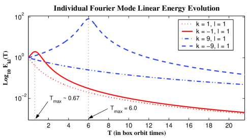
Figure 1: The behavior of the linear mode energy, $E_{{}_{k\ell}}$, with respect to time (33) in the SC frame is plotted for several $k$ and $\ell$ Fourier modes. Each mode begins with the same energy at $T=0$. Transient growth is strongest when the value of $|k/\ell|$ is largest (see the definition of $\vartheta_{k\ell}$ in Eq. 34). The times of maximal growth ($T=T_{{\rm max}}$) in the TG modes are also labelled.

4 2D Nonlinear Behavior

4.1 Equations Solved and Numerical Method

We consider fully nonlinear two dimensional disturbances (1-3 with $\partial_{z}=0,w=0$ and $\rho^{\prime}=0$) of the fluid with periodic boundary conditions in the SC frame. The equations of motion for the disturbances are evolved using the streamfunction-vorticity formulation discussed in the previous sections. The full nonlinear equations in the NSC frame are,

$$\partial_{t}\xi-qx\partial_{y}\xi+\partial_{y}\psi\partial_{x}\xi - \partial_{x}\psi\partial_{y}\xi=$$ (36)

$${\rm Re}^{-1}\left(\partial_{x}^{2}\xi+\partial_{y}^{2}\xi\right),$$

$$\partial_{x}^{2}\psi+\partial_{y}^{2}\psi = \xi.$$ (37)

When the transformations defined by (16) are applied, the equations in the SC frame are,

$$\partial_{{}_{T}}\xi+\partial_{{}_{Y}}\psi(\partial_{{}_{X}}\xi + qT\partial_{{}_{Y}}\xi)-\partial_{{}_{Y}}\xi\left(\partial_{{}_{X}}\psi+qT\partial_{{}_{Y}}\psi\right)=$$ (38)

$${\rm Re}^{-1}\left[\partial_{{}_{Y}}^{2}\xi+\left(\partial_{{}_{X}}+qT\partial_{{}_{Y}}\right)^{2}\xi\right],$$

$$\partial_{{}_{Y}}^{2}\psi+(\partial_{{}_{X}} + qT\partial_{{}_{Y}})^{2}\psi=\xi,$$ (39)

where we have added here, for the first time, an explicit viscous term to the equations. Specifically, the equations contain now a parameter (the Reynolds number). The purpose of this inclusion is to investigate how the flow behavior depends on Re and what influence Re has on the transition to the RTG state. For the most part, however, we report on inviscid results here, that is, with formally Re $=\infty$ in the above equations. We note that the numerical procedure implemented (see below) has a certain amount of artificial dissipation associated with it so that though the Re number may be infinite, it is so only nominally.

Doubly periodic boundary conditions are imposed upon all the quantities in the SC frame. This is identical with the conditions used by Hawley, Gammie & Balbus (hgb (1995)).

Equations (38-39) are solved using standard Fourier spectral methods (Canuto, et al. canuto (1988)) except for a number of details discussed below. Runs were performed usually on specific periodic domains ($L_{x}$,$L_{y}$) = ($\pi,2\pi$). Because the nonlinearities are quadratic, a 3/2 dealiasing rule is imposed (i) at each time step, after the nonlinear terms are computed and (ii) prior to each remapping event (see below). Aliasing problems can be especially hazardous here because one can inadvertedly transfer power from decaying (trailing) modes into transiently growing (leading) modes and create a situation in which there is spuriously generated RTG behavior. The dealiasing procedure outlined above satisfactorilly avoids this problem.

The Fourier resolution typically utilized 256 modes in $Y$ and $512$ modes in $X$. Convergence of the numerical scheme was verified by comparing the results of representative runs with those of an even higher resolution simulations (e.g. at $512\times 1024$). These numerical tests convince us that the 256$\times$512 spatial resolution is satisfactory for our purposes at this stage.

The governing PDE’s were temporally evolved using a modified Crank-Nicholson method described in Appendix B.

The domain in the $x=X$ direction nominally lies between $X=0$ and $X=L_{x}$. In the NSC frame, the background flow is not moving at $x=0$ while it moves with speed $qL_{x}$ at $x=L_{x}$. Consequently this means that the shear carries all the $y$ points at $x=L_{x}$ back to their initial starting position after a time $T_{rm}$ defined to be

$$T_{rm}=\left|\frac{L_{y}}{qL_{x}}\right|.$$ (40)

However, as noted in Hawley, Gammie & Balbus (hgb (1995)), points, as carried by the shear, are not always periodic in $x$: they are so only after every integer multiple of $T_{rm}$.

Thus, following the general prescription provided for by Cabot (cabot (1996)), the computational domain is remapped after every $T_{rm}$ period of time according to the following prescription:

1. At $T=t=0$ initial vorticity (or streamfunction) data are assumed to be known and given in the NSC frame. At this time the NSC ($x,y,t$) and SC ($X,Y,T$) are coincident.

2. Given this coincidence of both coordinate systems, the initial NSC data are used as the seed vorticity (or streamfunction) that evolve by (38) and (39), the equations in the SC, up to time $T=T_{rm}$.

3. Because only at $T=T_{rm}$ (and every integer multiple thereof ) are solutions exactly periodic in the $x$ direction of the NSC frame, at $T=T_{rm}$ the solution in the SC frame is mapped back into the NSC frame by applying the inverse transformation of (16) onto the modes in Fourier space according to the procedure in Appendix C, section 2. This act is what we will refer to as remapping.

4. We can treat the mapped, exactly periodic, solution in the NSC frame as the new initial condition to evolve (38-39) which, of course, is in the SC frame. Time in SC is reset to zero, i.e. $T=0$. The procedure repeats with item 2. Note that though $T$ is reset, time in the NSC still continues onward. For instance, at the $n^{{\rm th}}$ remapping, $T=0$ while $t=nT_{rm}$.

This procedure simply amounts to taking a solution that has been evolved in the SC and re-expressing it in terms of the coordinates of a normal (that is, in NSC) observer. Then the data as seen by the normal observer is used again as initial conditions for the next spate of evolution in the SC frame. It should be noted that if there were infinite resolution at our disposal, the remapping procedure mathematically effects nothing since it is a simple coordinate transformation. The rationale for applying the remapping procedure is technical: it involves issues concerning finite resolution, periodic boundary conditions, and the ability of resolving coherent structures for an extended period of time in the SC frame. For more details we refer the reader to Cabot (cabot (1996)) and to the discussion presented in Appendix C. Prior to each reemapping act, the state of the solution is padded using the similar 3/2 dealiasing procedure (see above). Failing to do this can introduce an aliasing error in which a decaying (trailing) Fourier mode can spuriously turn into a transiently growing (leading) Fourier mode (cf. end of section 3.1). Nonetheless, we have also performed a comparison run to see whether or not the recurrent transient growth we observe in the nonlinear solutions (see section 4.3) indeed persists when remapping is not done. Aside from slight differences in the evolution of the total disturbance energy and the differences in the enstrophy (when remapping is applied enstrophy decay is expected and observed while when no remapping is performed enstrophy conservation is predicted and observed), the observed recurrent dynamical phenomena persists in the non-remapped case just as it does in the simulations where remapping is done.

We define the parameter $\varepsilon$ to be a rough measure of what we shall call the turbulence intensity of the system. In particular we identify it to be the ratio of the domain integrated energy contained in fluid disturbances (i.e. the energy $E_{d}$ as defined by Eq. 35) to the domain integrated energy contained in the steady shear flow itself. The latter is the domain integral defined by

$$E_{shear}=\frac{1}{2}\int{\bf U}^{2}dxdy=\frac{1}{2}\int q^{2}x^{2}dxdy=\frac{1}{6}q^{2}L_{x}^{3}L_{y}.$$ (41)

The turbulent intensity is then formally written as,

$$\varepsilon=\frac{E_{d}}{E_{shear}}=\frac{6E_{d}}{q^{2}L_{x}^{3}L_{y}}$$ (42)

All simulations in this work, unless otherwise noted, begin with white noise in the vorticity field with a value of $\varepsilon$ always less than $0.01$. That is to say, the energy in the disturbances are always less than one percent of the total energy in the steady shear.

4.2 Disturbance energy and enstrophy evolution

To gain a certain amount of intuition for the underlying processes and to monitor the performance of our numerical technique we consider the evolution of the domain integrated energy of the disturbances. It is a straightforward matter to show that in the SC the following holds,

$$\frac{dE_{d}}{dT}=\left.q\int uvdXdY-Re^{-1}\int|\tilde{\nabla}u|^{2}dXdY\right.,$$ (43)

where the operator $\tilde{\nabla}$ is given as $\{\partial_{X}+qT\partial_{Y}\}{\bf\hat{X}}+\partial_{Y}{\bf\hat{Y}}$ and the integrals are taken over the periodic domain. The result in (43) is known in more general terms as the Reynolds-Orr relationship. When Re is finite it clearly demonstrates the decaying behavior due to viscosity since the second term on the RHS of (43) is a negative definite quantity. In the limit where Re is so large that the viscous decay time scale is very long, the evolution of $E_{d}$ is governed by the first term on the RHS of (43). It says that for $q>0$ ($<0$) there will be a rise in the integrated kinetic energy of the domain if there exists a positive (negative) correlation between the shearwise and streamwise velocities. From (43) it can be shown that the instantaneous relative growth rate of the disturbance energy, that is, $d\ln E_{d}/dt$ is independent of the amplitude (see Hennigson 1996). Thus the growth rate of a finite amplitude disturbance is essentially given by mechanisms present in the the linearized equations. Without linear growth mechanisms there can be no growth even in the nonlinear regime. Nonlinear processes can only shift power among the modes and this, as we shall explain below, is a key feature in understanding our results.

Additionally we also consider the enstrophy,

$${\cal Z}\equiv\int\small\mbox{$\frac{1}{2}$}\xi^{2}dXdY.$$ (44)

It too is a straightforward matter to show that this quantity follows

$$\frac{d{\cal Z}}{dT}=-{\rm Re}^{-1}\int|\tilde{\nabla}\xi|^{2}dXdY.$$ (45)

Thus ${\cal Z}$ always shows decay for finite Re, irrespective of the linear shear, and, it is only when Re = $\infty$ is ${\cal Z}$ conserved. In the Re = $\infty$ results we get, the enstrophy is indeed conserved between remapping events but, as is discussed in Appendix C, the act of remapping always removes enstrophy. The majority of this enstrophy is removed from very large wavenumber shearwise directed Fourier modes and since these contain very little of the energy - the overall effect on the global energetics are minimal.

4.3 Results: RTG and Coherent Vortices

We have conducted a number of runs for various values of the Reynolds number and initial conditions (the spectral structure of the disturbance was always the same, but we have varied the initial intensity, $\varepsilon(0)$). Generally speaking, we have found RTG behaviour for Reynolds numbers above some threshold. In some cases (not high enough Reynolds number or too small disturbance strength) the RTG was transient, ultimately decaying after a finite time (whose size depended on the two parameters mentioned above). Inviscid runs (Re=$\infty$ nominally) seeded with initial $\varepsilon=0.01$ displayed RTG displaying only an insignificant decay in times of the order of the run duration. Consider first Fig. 2, which shows the results of a Re = 50,000 run, demonstrating the persistence of RTG phenomenon in the time segment between $\sim 70$ and $\sim 170$. Long after the linear evolution of the initial conditions have died away, the nonlinear behavior shows quasi-steady long-lived activity, characterstic of what we have called RTG. Guided by the consequences of the Reynolds-Orr relationship (see the discussion following Eq. 43) we have performed numerical experiments which demonstrate that the peaks in the time evolution are actually driven by linear TG. We are led to this proposition by the results of the following experiments. At several time points during the late evolution of the flow, which are found (in the fully nonlinear simulation) to lie just before a growing peak, the state of the full flow is read and used as initial conditions for a parallel numerical evaluation of the linear behavior. This exercise reveals that the linear and nonlinear disturbance energy fluctuations of the full system, at least locally in time (between 5 and 10 time units), are nearly the same. Eventually the linear flow decays (as it should) while the nonlinear flow eventually demonstrates TG again. This quality is demonstrated in Fig. 2 for seven separate starting points.

As stated at the outset, we find that the repeated linear TG fluctuations in the total disturbance energy is a generic feature of the flows that have been numerically investigated by us. The only limitation appears to be whether or not there is sufficient power in those set of modes of the system that are transiently growing. For instance, we ran a simulation (not shown) in which all the disturbance energy was distributed amongst modes that cannot transiently grow. The resulting nonlinear dynamics showed fast decay exactly in line with linear theory.

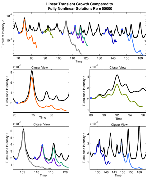
Figure 2: Full nonlinear evolution of disturbance energy at Re = 50000. Also plotted is the linear evolution of disturbances whose initial condition is the fluid state of the nonlinear solution at the specified times t = 70.0, 88.0, 102.6, 109.3, 112.0, 133.3, 146.7. These linear start times are indicated on the plots by diamonds. Though the full solution show strong nonlinearly, the linear evolution shows that the rises and falls of the total energy appear to be dominated by the linear TG process.

It is also important to note already here that these systems, in which sustained RTG is shown, posses an interesting spatial characteristics. The random initial vorticity disturbance develops into collections of coherent long-lived vortices which, once developed, translate in the streamwise direction with the speed of the local shear profile. It also appears that the number of emerging structures, showing temporal persistence, is a function of the box size in the shearwise (i.e. disk radial) direction only. This behavior is further detailed below.

We turn now to a more detailed description of fully inviscid (save only for numerical viscosity effect because of finite resolution and remapping) runs. As said before, these runs show RTG persisting for the full duration of our calculations. Three parallel evolution calculations of three nearly identical flows at Re $=\infty$ were performed. We refer to each of these ”runs” as ”a” , ”b” and ”c” and their parameters, describing only differing periodic box scales, are the following:

Run a: 

$L_{x}=\pi,L_{y}=2\pi$,

Run b: 

$L_{x}=2\pi,L_{y}=2\pi$,

Run c: 

$L_{x}=\pi,L_{y}=4\pi$.

Runs b and c are seeded with the initial data of Run a with some additional very weak perturbations.

Fig. 3 depicts the evolution of the quantity $\varepsilon$ for Run a. As before we see that the system demonstrates RTG phenomenon and the energetics of the system remain active far after the linear evolution (not shown) predicts decay. After the initial spectrum of decaying modes has died away ($T<50$), the system’s energy reaches a quasi-steady long-term sustained level. The same temporal features described here are observed with Runs b and c.

By comparison, we have also computed the evolution of a viscous version of Run a with Re = 50,000. This run demonstrated significant decay of the energy already by $T=350$ (which was the point where the simulation was stopped). The mix between decay and RTG activity is clearly evident in both runs here and falls in line with implications of the Reynolds-Orr relationship (43).

We now turn to the description of the spatial features of the results. By $t=100$ or so, each of the three runs settle down into a quasi-steady state described as a collection of coherent vortical structures that propagate along with the imposed streamwise flow. These structures appear (Fig. 4 & 5) to be long-lived in that they neither transiently decay nor do they become swallowed up by other vortices (see below) for the duration of the simulations (up to nearly $t\sim 800$). In this steady state Runs a and c support 3-5 coherent vortices while Run b supports about 7-8 coherent vortices.

Fig. 4 is representative of the long time spatial behavior in all the numerical simulations we have performed. It depicts the result of prolific vortex-vortex consumption leading to the production a single intermediate sized coherent structure. All simulations show that while the quasi-steady state is achieved, small to medium sized vortices having emerged at closely neighboring values of $x$ eventually consume each other because the background shear invariably advects the once-separated structures into each others vicinity. Many structured vortices may survive into the quasi-steady phase of the evolution but only one vortex will be associated with any streamline. The vortex merging feature observed here is not unexpected since this sort of thing has been observed in other 2D numerical investigations and has been discussed at length by McWilliams, (mcwilliams84 (1984)), Marcus (marcus93 (1993)) and more recently by Lin et al. (lin2003 (2003)). The comparison to these results (and thus testing our scheme) was our motivation in running the above three runs, differing only in the computational domains (see also below).

There are two main difference in the simulations between the finite and infinite Re cases. First, as shown above, all finite Re simulations show decay of their activity even though the interim dynamics are of the RTG type seen in the inviscid cases. In these latter cases (Re=$\infty$) the decay times in the total energy are essentially infinite since no decay was measurable for the duration of the runs. In these cases, any decay can be caused only by the numerical dissipation attributed to the remapping procedure (see discussion in Appendix C). Second, vortices appearing in the finite Re situations are less centrally concentrated than their counterparts in the ${\rm Re}=\infty$ cases. Fig. 6 shows this differing quality between two versions of Run a comparing ${\rm Re}=\infty$ and ${\rm Re}=50,000$.

In summary, the results show that (a) in the comparison runs between domains $L_{y}=4\pi$ and $L_{y}=2\pi$ (with $L_{x}=\pi$ in both), roughly the same number of vortices survive and (b) in the comparison runs between the domains $L_{x}=\pi$ and $L_{x}=2\pi$ (with $L_{y}=2\pi$ in both) the number of surviving vortices is nearly double in the $L_{x}=2\pi$ run. These findings offer qualitative support to the hypothesis, as suggested by P. Marcus (in conversation with one of the authors), that the number of emerging coherent structures is only a function of the size of the domain in the shearwise (disk radial) direction and that, further, no more than one sizeable long-lived vortex can occupy the same radial neighborhood or zone. Of course, the generality and veracity of this assertion needs to be evaluated with further systematic studies.

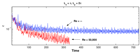
Figure 3: The quantity $\varepsilon$ for Run a: white noise initial conditions for the vorticity, $L_{x}=2\pi,L_{y}=2\pi$. A viscous (Re = 50,000) and inviscid flow, (${\rm Re}=\infty$) are depicted for comparsion. Aside from the initial transient readjustment phase ($T<50$), the inviscid run demonstrates no decay over the course of its duration.

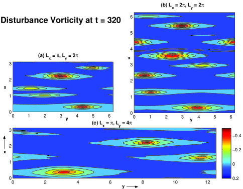
Figure 4: The vorticity distribution at $t=320.0$ as viewed by a non-sheared observer for Runs a,b,c at Re = $50,000$. In each figure a quasi steady state has been reached by the solutions. In (a) between 3-5 vortices survive while in (b) 7-8 vortices persist. In (c) about 3 vortices survive. The results are suggestive of the hyptothesis that the number of surviving vortices is a function of the radial ($\hat{x}$ direction) domain size and that for any given streamline there is only one coherent vortex associated with it.

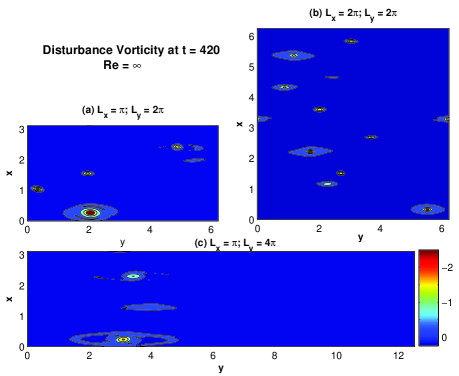
Figure 5: Same as Fig. 4 except that Re = $\infty$. The concentration of vorticity is tighter than in the viscous case.

Figure 6: Surface plot of the vorticity at long times. Comparison between Re = $50,000$ (top panel) and Re = $\infty$ (lower panel). The concentration and amplitude of the vorticity in the Re = $\infty$ case is tighter than in the viscous case.

5 Discussion and Summary

5.1 The shearing box approximation, its limits and properties

We have presented semi-rigorous scaling arguments in order to derive appropriate equations for describing small-scale dynamics in the midplane vicinity of rotationally supported thin barotropic disks. The procedure admits two limits, the SSB and the LSB, whose choice depends on the length scales of interest. In this work we work with the SSB equations, because in this first study we limit our interest to dynamical lengths which are small compared to the vertical scale-height of the disk. In this way we obtain a simpler problem, avoiding the complications resulting from the inclusion of acoustic modes. The SSB equations are essentially that of incompressible fluid flow in a homogenously shearing environment with constant Coriolis parameter. In fact, in both the LSB and SSB scaling limits the Coriolis parameter is a local constant and the shear is homogenous. However, by using a shearing box approximation (which utilizes the asymptotic scaling constants $\epsilon$ and $\delta$ - see Appendix A), a physical scale in the disk is set. It appears thus that the argument of Balbus (2003) (regarding the above mentioned Longaretti’s speculation on the numerical resolution needed to see instability in rotating flows) is not well founded.

The asymptotic equations describing the two shearing box scalings, as derived in the Appendix A, relate to those used elsewhere in the literature. The SSB equations, in their linearized form, are the same as those used by Chagelishvili et al. (chag (2003)). Identical equations, i.e. describing the SSB with no a priori density fluctuations, are also equivalent to the ones usually used in the fluid dynamics community to investigate inviscid incompressible rotating plane Couette flow (Nagata, nagata (1986)). In their full nonlinear form, the equations for the SSB are equivalent to the equations cited by Longaretti (longaretti (2002)) where the density disturbances are everywhere zero.

The equations describing the LSB admit acoustic disturbances unlike the SSB limit. In their linearized form, the equations in the LSB are only similar to the equations used by Tevzadze et al. (tevzadze (2003)) where, in their work, steady state pressure gradients are assumed to be uniform rather than having the positional dependence they are understood to have for barotropic pressure profiles, cf. (65) and (66). The fully nonlinear equations of the LSB are similar to those used by BHSW except that in their treatment the steady density and pressure profiles are considered to be uniform (avoiding vertical structure effects). This seems to be, thus, a kind of an intermediate limit between our SSB and LSB.

5.2 TG: its linear decay and its nonlinear reccurrence

Both the finite and infinite Re number simulations described in this work show that long after linear theory predicts the decay of all disturbances, the total disturbance energy exhibits repeated episodes of transient growth. This is established by considering the parallel linear evolution of the nonlinear state at various points in time. The condition of the full nonlinear flow is used as the initial condition for the linear evolution and we find that the linear and nonlinear development closely shadow each other for at least 5 time units. Where there is linear TG the full flow also demonstrates TG. Fig. 3 qualitatively indicates that the temporal pattern in the RTG is complex and appears to be chaotic.

Whether a similar result can be expected in 3D, despite BHSW repeated claims that this is impossible, must be decided by 3D simulations. Recent simulations of 3D plane Couette flows (without rotation) at relatively low Re-numbers by Schmiegel and Eckhardt (schmiegel (1997)) show similar (to the one described here) behavior of the integrated domain energies. While eventual decay is observed in most cases, the fluid response is chaotic in the interim. They further show that simulations with the same total initial energy and Re numbers but with differing initial conditions can exhibit vastly differing decay timescales - and in some instances there is no dissipation over the duration of a simulation (Eckhardt, Marzinzik & Schmiegel 1998). Though not reported here in detail, we also observe similar sensitivity to initial conditions for simulations with finite Re numbers in the way described in their work. A detailed exposition of these results will be reported in our future work.

Though the detailed nonlinear feedback mechanism has not yet been identified it seems apparent to us that the linear TG phenomenon is a central player of this dynamical system and is a key element in the dynamics of rotationally supported flows like thin Keplerian disks. The findings of this work also lend support to the conjectures put forth by Baggett, et al. (baggett (1995)), Waleffe (waleffe (1997)), and more recently Grossmann (grossmann (2000)): that subcritical flows, in the sense that there are no linearly unstable processes, are governed by an interplay between linear TG and some sort of nonlinear feedback of energy back onto TG modes.

5.3 Coherent structures

Our results have some bearing on certain fundamental questions pertaining to 2D turbulence. In the work of McWilliams (1984), in which simulations of 2D non-globally sheared geostrophic flows were performed, it was shown that vorticity concentrations at intermediate scales exhibit long lifetimes: i.e. times that are long compared to their eddy-turnaround times and with sizes larger than the dissipation scales. This result inspired the hypothesis that it is a typical feature for two-dimensional geostrophic flows to sustain these types coherent vortices and, further, for them to retain their independence and identity unless there is a close (and usually destructive) encounter with another vortex. Additional support for this view was reported by Bracco et al. (bracco (2000)) using very high resolution 2D simulations of the same problem. The appearance and persistence of vortices at intermediate scales of the computational domain in our work qualitatively falls in line with the suggestion that the persistence of intermediate scale vortices are a generic feature of these sorts of flows.

Furthermore, the appearance of widespread merging of smaller vortices leading to the formation of intermediate scale quasi-steady structures is also consistent with what has been observed in the previously mentioned non-globally sheared simulations by McWilliams and Bracco et al.; and also those of the 3D shearing simulations of Lin et al. (lin2003 (2003)). What the results of this work add to the emerging picture of such flows is that with a globally imposed shear, intermediate sized vortices not only may appear and persist for a long time but they also tend to be solitary. In other words, multiple vortices may initially emerge but once the quasi-steady state is reached and most of the vortex-vortex merging/destruction events have taken place, a given point in the shearwise direction $x$ (irrespective of any streamwise position $y$) will have only one sizable coherent vortex associated with it . This pattern is consistent with the speculations made to this end by P. Marcus (private communication).

We find it somewhat encouraging that the number of emerged quasi-steady vortices increases when the domain size in the radial direction is increased. It suggests strongly that the emergence of coherent structures in such flows is an intrinsic phenomenon and it is not, say for instance, a by-product of the boundary conditions used. By this we mean to say that if at the end of our simulations we were to find that only one or two large scale vortices survived into the quasi steady state stage irrespective of the size of the computational domain in the shearwise direction, then we would probably feel that the pattern of developing and sustained coherence would not be indicative of phenomena intrinsic to these flows but rather an artifact of the boundary conditions employed (those here being SB periodicity).

5.4 Summary

Though the numerical results reported in this work are exclusively of two dimensional nonlinear simulations, we think that they may contribute to the understanding of subcritical transition in more general shear flows as well (including rotating ones). We have found here support to the idea that excepting the special circumstance, where initial conditions are set up via conspiracy (in the sense of the phrase as used by Goldreich & Lynden-Bell, goldreich65 (1965)) to have no spectral power in TG modes, these 2D flows are likely to be dynamically active and to exhibit and maintain robust vortices. Indeed, in viscous 2D flows such activity must invariably be limited to finite times, after which such activity and the associated vortices will decay. Nonetheless, accretion disk Reynolds numbers are enormous - much larger than those arising from numerical roundoff in our calculations. As such, we may expect correspondingly enormous decay times (already larger than the several hundred box orbit times of our simulations) during which the occurrence of new perturbations can not be excluded.

It is thus reasonable to still seriously consider the hypothesis that thin Keplerian disks may be hydrodynamically active, where the activity we envisage is of the RTG kind. It still remains to be seen, of course, whether or not three dimensionality and its introduction of stratification and Coriolis effects in rotating flows significantly alters the implications of our results.

Based on the results of their simulations, BHSW strongly advocate just that, but our work indicates that this issue deserves additional consideration. In particular, we are now engaged in extending our simulations to 3D, where different numerical schemes (spectral methods) in high spatial resolution and long integration times are employed. The effects of stratification and compressibility are also being addressed. Since we have found here that the initial conditions may be crucial in determining the persistence time of RTG, we intend to experiment with a variety of these and ascertain optimal perturbations. The results of these simulations may decide the important and still controversial issue if complex dynamical turbulence-like activity may be driven by purely hydrodynamical processes of the RTG kind in rotationally supported thin circumstellar disks.

6 Acknowledgements

The authors thank the anonymous referee for his suggestions that which helped us improve the presentation of our ideas and results. The authors would also like to thank the Israeli Science Foundation for making this work possible. We also thank Jeff Cuzzi, Sandy Davis and Denis Richard at NASA Ames Research Center for their useful comments and for a critical suggestion they made to us. We are grateful to Ed Spiegel and Giora Shaviv for their willingness to discuss with us the issues of this paper and for sharing with us their insights.

Appendix A Derivation of the Shearing Box (SB) approximation equations

The shearing box (or sheet) (SB) approximation has been used in a variety of astrophysical applications. It appears that the studies of Hill (1878) on lunar dynamics have provided the basic ideas for its development. The approximation has more recently been utilized by Goldreich & Lynden-Bell (1965) and Toomre (1981) in the context of galactic disks, Wisdom & Tremaine (1988) in the study of planetary rings, Goodman & Ryu (1992)for accretion disks and by Hawley, Gammie & Balbus (1995) in the study of magnetized accretion disks. It is within this approximation that most of the works mentioned in the Introduction have been done and it is used in this and our subsequent works. It is important, in our view, that all the approximations made in deriving the SB equations in their various limits be precisely spelled out and clarified and this is the purpose of this Appendix.

A.1 Global equations in a rotating frame, cylindrical coordinates

We start with the hydrodynamical equations, describing an ideal fluid (actually an inviscid and isentropic flow), in cylindrical coordinates (unit vectors $\hat{\bf r},\hat{\mbox{\boldmath$\mbox{\boldmath$\varphi$}$}},\hat{\bf z}$) and in a frame of reference rotating with a given angular velocity $\Omega_{0}\hat{\bf z}$ (see below). The only body force acting on the fluid is the gravitational attraction of a point mass $M$, located at the origin. The equation of state is assumed to be one of a perfect gas with constant adiabatic coefficient $\gamma$. The equations of mass momentum and energy conservation are then

$$\partial_{t}\rho+\nabla\cdot(\rho{\bf w}) = 0,$$ (46)

$$\partial_{t}{\bf w}+({\bf w}\cdot\nabla){\bf w}+2\Omega_{0}(w_{r}\hat{\mbox{\boldmath$\mbox{\boldmath$\varphi$}$}}-w_{\varphi}\hat{\bf r}) = -\frac{1}{\rho}{\nabla P}-r\Omega_{0}^{2}\,\hat{\bf r}-\nabla\phi,$$ (47)

$$\partial_{t}P+({\bf w}\cdot\nabla)P+\gamma P\nabla\cdot{\bf w} = 0,$$ (48)

where $\rho,{\bf w}$ and $P$ are the density, velocity and pressure fields respectively and $\phi(r,z)$ is the gravitational potential which is explicitly given by $\phi(r,z)=GM(r^{2}+z^{2})^{-1/2}$.

Before making the crucial step in the derivation of the SB equations (i.e. considering a small region around a point and deriving the local equations valid approximately in this region) we note that for any given rotation law $\Omega=\Omega(r)$, there exists a steady axisymmetric solution, with the pressure satisfying a global barotropic relation (i.e. being a well defined function of $\rho$ - $P=P(\rho)$) and the velocity being composed of the rotation only, that is ${\bf w}=r\,[\Omega(r)-\Omega_{0}]\,\hat{\mbox{\boldmath$\mbox{\boldmath$\varphi$}$}}$, as expressed in the rotating frame (see e.g. Tassoul & Tassoul 1978). Denoting by $\rho_{b}(r,z)$ the density in this solution for a given rotation law $\Omega(r)$ we can express the gravitational force per unit mass as follows

$$\nabla\phi=-\frac{1}{\rho_{b}}\nabla P_{b}+r\,\Omega^{2}\hat{\bf r},$$ (49)

where $P_{b}(r,z)$ is obtained from $\rho_{b}$ by the barotropic relation. Relation (49) allows one to substitute for the gravity term in (47) and we shall do it below. It is important to notice that if the rotation law $\Omega(r)$ is close to the Keplerian one and the disk the fluid is cold enough (that is the vertical scale height is small), the steady solution is an essentially rotationally supported disk.

A.2 Local nondimensional box equations in a rotating frame, Cartesian coordinates

We concentrate now on a small region around a point ${\bf r}_{0}$ - ($r=r_{0}$, $\varphi=\varphi_{0}$, $z=0$) - , that is, some typical point in the midplane of our disk. Let the region be of size $\Delta$, so that it (henceforth referred to as the box) is defined by

$$r_{0}-\frac{\Delta}{2}\leq r\leq r_{0}+\frac{\Delta}{2};\leavevmode\nobreak\ \leavevmode\nobreak\ \leavevmode\nobreak\ \leavevmode\nobreak\ \leavevmode\nobreak\ \varphi_{0}-\frac{\Delta}{2r_{0}}\leq\varphi\leq\varphi_{0}+\frac{\Delta}{2r_{0}};\leavevmode\nobreak\ \leavevmode\nobreak\ \leavevmode\nobreak\ \leavevmode\nobreak\ \leavevmode\nobreak\ -\frac{\Delta}{2}\leq z\leq\frac{\Delta}{2},$$

where $\delta\equiv\frac{\Delta}{r_{0}}\ll 1$.

The smallness of $\delta$ allows the employment of Cartesian coordinates, since locally the curvature in the azimuthal direction is only slight and, as we shall see below, drops out at lowest order in $\delta$. Thus we can transform the coordinates

$$x\equiv r-r_{0},\leavevmode\nobreak\ \leavevmode\nobreak\ \leavevmode\nobreak\ \leavevmode\nobreak\ \leavevmode\nobreak\ y\equiv r_{0}(\varphi-\varphi_{0});$$ (50)

and effect this transformation on equations (46-48), with the gravitational term in (47) substituted from (49).

Before writing out these equations in detail we nondimensionalize them, because only then we will be able to systematically neglect terms which are of higher order in the small parameter $\delta$. Thus $x,y,z$ are scaled by $\Delta=\delta r_{0}$, $t$ by the Kepler time at $r_{0}$, $\tau_{K}=\Omega_{K}^{-1}(r_{0})\equiv\sqrt{r_{0}^{3}/(GM)}$, $\Omega$ by $\Omega_{K}(r_{0})$, $\rho$ by $\rho_{0}\equiv\rho_{b}(r_{0},\varphi_{0},0)$, $P$ by the corresponding $P_{0}$ and the velocities by $v_{0}\equiv\Omega_{K}\Delta=\delta\Omega_{K}(r_{0})r_{0}$. Note that the velocity scale is related to the typical local sound speed scale, $c_{s0}\equiv\sqrt{P_{0}/\rho_{0}}$ by the relation

$$v_{0}=\frac{\delta}{\epsilon}c_{s0},$$

where $\epsilon\equiv c_{s0}/[\Omega_{K}(r_{0})r_{0}]$ and thus $H\equiv\epsilon r_{0}$ is the local vertical scale-height of the disk. In cold disks, by definition $\epsilon\ll 1$ and thus they are thin. We assume throughout this discussion that disks are cold.

We do not specify for the moment the order of magnitude of the ratio of the small parameters $\delta$ and $\epsilon$. Their ordering will correspond, as we shall see later, to different physical regimes of the local problem. Thus keeping the two small parameters as they are, we obtain the following set of nondimensional equations, which are valid in the small box around the point ${\bf r}_{0}$:

$$\partial_{t}\rho+\nabla\cdot(\rho{\bf w}) = 0,$$ (51)

$$\partial_{t}w_{x}+({\bf w}\cdot\nabla)w_{x}-2\Omega_{0}w_{y}-2q\Omega_{0}^{2}x = -\left(\frac{\epsilon}{\delta}\right)^{2}\left(\frac{1}{\rho}{\partial_{x}P}-\frac{1}{\rho_{b}}{\partial_{x}P_{b}}\right),$$ (52)

$$\partial_{t}w_{y}+({\bf w}\cdot\nabla)w_{y}+2\Omega_{0}w_{x} = -\left(\frac{\epsilon}{\delta}\right)^{2}\frac{1}{\rho}{\partial_{y}P},$$ (53)

$$\partial_{t}w_{z}+({\bf w}\cdot\nabla)w_{z} = -\left(\frac{\epsilon}{\delta}\right)^{2}\left(\frac{1}{\rho}{\partial_{z}P}-\frac{1}{\rho_{b}}{\partial_{z}P_{b}}\right),$$ (54)

$$\partial_{t}P+({\bf w}\cdot\nabla)P+\gamma P\nabla\cdot{\bf w} = 0,$$ (55)

where we have kept only terms in lowest order in $\delta$ and therefore neglected the curvature terms, so that the above equations (that is, the vectors and derivatives) are actually expressed in local Cartesian coordinates, defined in (50). The net radial body force in the rotating frame $r(\Omega^{2}-\Omega_{0}^{2})$ has been expanded around $r_{0}$ up to order $\delta$, where $\Omega_{0}$ the rotational velocity of the frame is actually the value of the rotational law angular velocity at $r_{0}$, that is, $\Omega(r_{0})$ expressed in units of the Keplerian rotational velocity at that point. For Keplerian rotation law we obviously have $\Omega_{0}=1$. The parameter $q$ is related to the Oort constant $A$:

$$q\equiv-\left(\frac{d\ln\Omega}{d\ln r}\right)_{r_{0}}=-2\frac{A}{\Omega_{0}}.$$ (56)

In the terms on the right hand side of the momentum equations we have the differences between the pressure force components and the corresponding components in the basic steady barotropic state, referred to above. That barotropic state is clearly axially symmetric and thus $\partial_{y}P_{b}=\partial_{y}\rho_{b}=0$, but in the radial and vertical directions we can not expect a priori the uniformity the density and pressure.

Note, however, that because the ratio $(\epsilon/\delta)^{2}$ multiplies the pressure force terms in question, their size will have to be such as to allow for proper balancing of the equations (see below).

A.3 Removal of steady state linear shear - the shearing box (SB) equations for the perturbations

We notice now that ${\bf w}=2Ax{\bf\hat{y}}$, $P=P_{b}$ and $\rho=\rho_{b}$ is a steady solution of equations (51-55) and therefore we consider this solution as our basic flow and perturb it by adding functions of space and time (denoted by primed quantities). Thus we write

$${\bf w} = 2Ax{\bf\hat{y}}+{\bf u^{\prime}},$$ (57)

$$\rho = \rho_{b}+\rho^{\prime},$$ (58)

$$P = P_{b}+P^{\prime},$$ (59)

Substitution of the above form of the functions in the equations gives rise to the removal of the linear shear steady solution and the following equations for the perturbations ${\bf u}^{\prime}$, ${\rho^{\prime}}$ and $P^{\prime}$ are obtained:

$$\partial_{t}\rho^{\prime}+2Ax\partial_{y}\rho^{\prime}+\rho_{b}\nabla\cdot{\bf u^{\prime}}+u^{\prime}_{z}\,\partial_{z}\rho_{b}+u^{\prime}_{x}\,\partial_{x}\rho_{b}+\nabla\cdot(\rho^{\prime}{\bf u^{\prime}})=0,$$ (60)

$$\partial_{t}u^{\prime}_{x}+2Ax\partial_{y}u^{\prime}_{x}-2\Omega_{0}u^{\prime}_{y}+({\bf u^{\prime}}\cdot\nabla)u^{\prime}_{x}=-\left(\frac{\epsilon}{\delta}\right)^{2}\left(\frac{{\partial_{x}P^{\prime}}}{\rho_{b}+\rho^{\prime}}\,-\frac{\rho^{\prime}\partial_{x}P_{b}}{\rho_{b}^{2}+\rho_{b}\rho^{\prime}}\,\right),$$ (61)

$$\partial_{t}u^{\prime}_{y}+2Ax\partial_{y}u^{\prime}_{y}+2(A+\Omega_{0})u^{\prime}_{x}+({\bf u^{\prime}}\cdot\nabla)u^{\prime}_{y}=-\left(\frac{\epsilon}{\delta}\right)^{2}\left(\frac{{\partial_{y}P^{\prime}}}{\rho_{b}+\rho^{\prime}}\,\right),$$ (62)

$$\partial_{t}u^{\prime}_{z}+2Ax\partial_{y}u^{\prime}_{z}+({\bf u^{\prime}}\cdot\nabla)u^{\prime}_{z}=-\left(\frac{\epsilon}{\delta}\right)^{2}\left(\frac{{\partial_{z}P^{\prime}}}{\rho_{b}+\rho^{\prime}}\,-\frac{\rho^{\prime}\partial_{z}P_{b}}{\rho_{b}^{2}+\rho_{b}\rho^{\prime}}\,\right),$$ (63)

$$\partial_{t}P^{\prime}+2Ax\partial_{y}P^{\prime}+u^{\prime}_{x}\,\partial_{x}P_{b}+u^{\prime}_{z}\,\partial_{z}P_{b}+\gamma P_{b}\nabla\cdot{\bf u^{\prime}}+{\bf u^{\prime}}\cdot\nabla P^{\prime}+\gamma P^{\prime}\nabla\cdot{\bf u^{\prime}}=0.$$ (64)

where we have retained the full nonlinear terms, that is, did not expand in the perturbations.

This set of equations for the perturbations is quite general and it includes all the different cases which were used in the literature. The advantage of this formulation is in its consistency and physical transparency as to which approximations are made (see below).

A.3.1 Small shearing box (SSB) equations ($\delta\ll\epsilon\ll 1$)

When we chose $\delta\ll\epsilon$, the shearing box size is much smaller that the disk’s thickness (the unperturbed pressure vertical scale height). This choice implies that the pressure force terms in equations (61-63) are multiplied by a very large factor and therefore if we want that in the prevailing dynamics these terms be of the order of the inertial terms, they themselves must be of the order of $(\delta/\epsilon)^{2}$.

Consider first the terms containing the gradient of the steady barotropic pressure $P_{b}$. The $z$ derivative of $P_{b}$ (and thus of $\rho_{b}$ as well) is in our units clearly of the order $(\delta/\epsilon)^{2}$, because by nondimensionalizing equation (49) one gets that in the box

$$\frac{1}{\rho_{b}}{\partial_{x}P_{b}} = -\left(\frac{\delta}{\epsilon^{2}}\right)(1+\delta x)\left\{\Omega^{2}(x)-\left[(1+\delta x)^{2}+\delta^{2}z^{2}\right]^{-3/2}\right\},$$ (65)

$$\frac{1}{\rho_{b}}{\partial_{z}P_{b}} = -\left(\frac{\delta}{\epsilon}\right)^{2}z\left[(1+\delta x)^{2}+\delta^{2}z^{2}\right]^{-3/2},$$ (66)

where $\Omega(x)$ is the rotational nondimensional rotational velocity in the box.

The order of magnitude of $\frac{1}{\rho_{b}}{\partial_{x}P_{b}}$ depends on the rotation law. If the rotation law is exactly Keplerian, we have $\Omega^{2}(x)=(1+\delta x)^{-3}$ and $\frac{1}{\rho_{b}}{\partial_{x}P_{b}}={\cal O}\left({\delta^{3}/\epsilon^{2}}\right)$ and $\frac{1}{\rho_{b}}{\partial_{z}P_{b}}=-z\delta^{2}/\epsilon^{2}+{\cal O}\left({\delta^{3}/\epsilon^{2}}\right)$. More generally speaking, in order to have $\frac{1}{\rho_{b}}{\partial_{x}P_{b}}={\cal O}\left({\delta^{3}/\epsilon^{2}}\right)$, the basic rotation state does not have to be exactly Keplerian, but just close enough to it. In other words, order 1 departures from a Keplerian rotation profile are needed to see significant radial gradients of the steady state in this approximate limit.

Thus, assuming that the rotation law is close enough to the Keplerian (some special choices appear in the body of the paper), and for the sake of economy of the notation, we make the replacements

$$\partial_{i}P_{b}\to\left(\frac{\delta}{\epsilon}\right)^{2}\partial_{i}P_{b}$$ (67)

and

$$\partial_{i}\rho_{b}\to\left(\frac{\delta}{\epsilon}\right)^{2}\partial_{i}\rho_{b}$$ (68)

for $i=x,z$, remembering that the units of the barotropic profile spatial derivatives have been scaled accordingly.

Examine next the terms containing the perturbations $P^{\prime}$ in equations (61-63). If these are not sufficiently small (that is of order $\delta^{2}/\epsilon^{2}$) we may formally write

$$P^{\prime}=P^{\prime}_{0}+\left(\frac{\delta}{\epsilon}\right)^{2}p+...$$ (69)

With this expansion (and using the above scaling of the barotropic terms), equations (61-63) give in lowest order

$$\nabla P_{0}^{\prime}=0$$ (70)

that the ${\cal O}\left({1}\right)$ part of the pressure perturbation is uniform in the box. Using this in equation (64) gives in lowest order

$$\partial_{t}P^{\prime}_{0}=-\gamma\nabla\cdot[(P_{b}+P^{\prime}_{0}){\bf u^{\prime}}].$$ (71)

Integration of this equation over the volume of the box shows that the time variation of $P^{\prime}_{0}$ depends on the boundary conditions. For both periodic or zero velocity boundary conditions (which are usually employed) we get that $P^{\prime}_{0}$ is also constant in time. Thus this constant pressure shift may be formally absorbed into $P_{b}$ and consequently changing nothing. Thus we may now formally write

$$P^{\prime}\equiv\left(\frac{\delta}{\epsilon}\right)^{2}p,$$ (72)

in which $p$ is now understood to be an order one quantity. This actually amounts to redefining the units of the pressure perturbation.

Substitution of these scalings into (60-64) and dropping terms of ${\cal O}\left({(\delta/\epsilon)^{2}}\right)$ and smaller gives that the energy equation (64) simplifies to

$$\nabla\cdot{\bf u^{\prime}}=0,$$ (73)

that is, we are dealing in this approximation with an incompressible flow. This is physically consistent with the fact that the relative pressure perturbation was assumed to be very small. We have an incompressible flow with the density of any fluid element conserved by the flow and the the small pressure perturbations describe the dynamics of non-acoustic (that is solenoidal, or vortical) modes only.

The three momentum equations become:

$$\partial_{t}u^{\prime}_{x}+2Ax\partial_{y}u^{\prime}_{x}-2\Omega_{0}u^{\prime}_{y}+({\bf u^{\prime}}\cdot\nabla)u^{\prime}_{x} = -\left(\frac{1}{\rho_{b}+\rho^{\prime}}\,{\partial_{x}p}-\frac{\rho^{\prime}}{\rho_{b}^{2}+\rho_{b}\rho^{\prime}}\,\partial_{x}P_{b}\right)$$ (74)

$$\partial_{t}u^{\prime}_{y}+2Ax\partial_{y}u^{\prime}_{y}+2(\Omega_{0}+A)u^{\prime}_{x}+({\bf u^{\prime}}\cdot\nabla)u^{\prime}_{y} = -\left(\frac{1}{\rho_{b}+\rho^{\prime}}\,{\partial_{y}p}\right),$$ (75)

$$\partial_{t}u^{\prime}_{z}+2Ax\partial_{y}u^{\prime}_{z}+({\bf u^{\prime}}\cdot\nabla)u^{\prime}_{z} = -\left(\frac{1}{\rho_{b}+\rho^{\prime}}\,{\partial_{z}p}-\frac{\rho^{\prime}}{\rho_{b}^{2}+\rho_{b}\rho^{\prime}}\,\partial_{z}P_{b}\right)$$ (76)

Finally, the equation for the density perturbation $\rho^{\prime}$ results from (60) and, in this order, reads

$$\partial_{t}\rho^{\prime}+2Ax\partial_{y}\rho^{\prime}+{\bf u^{\prime}}\cdot\nabla\rho^{\prime}=0.$$ (77)

The set (73-77), supplemented by the appropriate boundary conditions (usually chosen to be periodic), describes the full nonlinear problem in the SSB approximation, that is, for $\delta\ll\epsilon$. These equations with $\rho^{\prime}=0$ throughout is equivalent to the system studied by Longaretti 2002 and is often times referred to and studied as rotating plane Couette flow (Nagata, nagata (1986)). The linear problem contains the one studied by Chagelishvili et al. (2002).

A.3.2 Large shearing box (LSB) equations ($\delta\sim\epsilon\ll 1$)

We chose now $\delta=\epsilon$ the size of the shearing box is of the order of the vertical thickness of the disk. In this case the relative size of pressure perturbations is of the order of the relative density perturbations (to balance the relevant terms) and the vertical and horizontal derivatives of the barotropic pressure are necessarily retained in all of the equations as well. When the flow is nearly Keplerian, only the vertical derivatives make it in at the lowest order as it was argued in the previous section. We get equations identical to the full set (60-64) but with $\delta=\epsilon$ and where, in practice, only the first order terms of the basic state barotropic profiles (65-66) survive to this lowest order. Unlike the SSB, in this limit acoustic waves will be included in the equations as the flow is not incompressible. We shall treat this system in future works.

It should be noted that Tevzadze et. al (2003) used a simplified version of the linear limit of these equations. The system studied by Balbus, Hawley and collaborators (for instance Eqs. 3.5a-b in Balbus, Hawley and Stone, bhs96 (1996)) is a special case of this problem with the background barotropic density and pressure profiles assumed to be uniform.

Appendix B Details of the nonlinear 2D numerical method

We begin with (38) and (39). We assume all quantities to be Fourier-Galerkin expanded in both the $X$ and $Y$ directions. For example we have for the vorticity,

$$\xi=\sum_{k,\ell}\xi_{{}_{k\ell}}(T)e^{ikX+i\ell Y};$$ (78)

we similarly expand in this way for the stream function $\psi$. Note that each In the Fourier basis the equations are in which the Jacobian $J$ is

$$J(\psi,\xi)=\partial_{{}_{Y}}\psi(\partial_{{}_{X}}\xi+qT\partial_{{}_{Y}}\xi)-\partial\xi_{{}_{Y}}(\partial_{{}_{X}}\psi+qT\partial_{{}_{Y}}\psi).$$ (79)

Like $\xi_{{}_{k\ell}}$, $J_{{}_{k\ell}}$ references the $k,\ell$ Fourier component of the Jacobian. The time stepping is done via a modified Crank-Nicholson method outlined below. We write the above equation in the more generalized form,

$$\frac{d\xi_{{}_{k\ell}}}{dT}=-J_{{}_{k\ell}}+{\cal L}_{{}_{k\ell}}(T)\xi_{{}_{k\ell}},$$ (80)

where the linear operator ${\cal L}_{{}_{k\ell}}$ acting on Fourier component $\bf k$ has an explicit $T$ dependence. The evolution scheme time centers the evaluation of the nonlinear term $J_{{}_{k\ell}}$ and uses a time averaged evaluation of the linear operator. If superscript $n$ refers to the $n^{{\rm th}}$ time step and if $\delta t$ refers to the time difference between successive time steps then the temporal discretization of (80) becomes,

$$\frac{\xi^{n+1}_{{}_{k\ell}}-\xi^{n-1}_{{}_{k\ell}}}{2\delta t}=\frac{{\cal L}_{{\bf k\ell}}(T+\delta t)\xi^{n+1}_{{}_{k\ell}}+{\cal L}_{{\bf k\ell}}(T-\delta t)\xi^{n-1}_{{}_{k\ell}}}{2}-J^{n}_{{}_{k\ell}}(T),$$ (81)

reshuffling terms gives,

$$\xi^{n+1}_{{}_{k\ell}}=\frac{1+\delta t{\cal L}_{{}_{k\ell}}(T-\delta t)}{1-\delta t{\cal L}_{{}_{k\ell}}(T+\delta t)}\ \xi^{n-1}_{{}_{k\ell}}-\frac{2\delta t}{1-\delta t{\cal L}_{{}_{k\ell}}(T+\delta t)}J^{n}_{{}_{k\ell}}(T).$$ (82)

We also remind the reader that $J^{n}_{{}_{k\ell}}$ is the Jacobian evaluated at the time step $n$. We notice that the terms involving the linear operator appearing in the above expressions are the first terms of a Taylor series expansion of their exponential forms. That is,

$$\exp\left\{\int_{T}^{T+\delta t}{\cal L}_{{}_{k\ell}}dT^{\prime}\right\}\approx 1+\delta t{\cal L}_{{}_{k\ell}}(T)+{\cal O}\left({\delta t^{2}}\right),$$ (83)

we replace all appearances of ${\cal L}_{{}_{k\ell}}$ with the above approximate form. Thus (82) becomes

$$\xi^{n+1}_{{}_{k\ell}}=\exp\left\{\int_{T-\delta t}^{T+\delta t}{\cal L}_{{}_{k\ell}}dT^{\prime}\right\}\xi^{n-1}_{{}_{k\ell}}-2\delta t\exp\left\{\int_{T}^{T+\delta t}{\cal L}_{{}_{k\ell}}dT^{\prime}\right\}J^{n}_{{}_{k\ell}}(T).$$ (84)

Replacing the linear operators as we have here is akin to a Pàde Approximation (Bender & Orszag, bender (1999)) except in reverse: we have “inferred” a more accurate form of the operator by recognizing that the fractional terms in (82) are the approximations of the exponentials which are the exact solutions to problems with such operators. This procedure more accurately represents the linear evolution and it removes the well-known high-wavenumber inaccuracies (though stable) associated with Crank-Nicholson methods: in particular, as originating from the denominators of (82).

Appendix C Remapping: its rationale and technical details

The original call to our attention of the ideas behind remapping is credited to P.S. Marcus who, in several private comminications with one of the authors (OMU), sketched out the essential rudiments of the problems (and their resolution) as they are discussed herein. To our knowledge, Cabot (cabot (1996)) is the only published work in the literature in which the steps describing the remapping procedure is both outlined and discussed with some detail.

C.1 The rationale

We have two goals in mind when developing (numerical) nonlinear solutions of (38) and (39):

1. to accurately implement periodicity in the SC frame (as in the programme outlined in Hawley et al., hgb (1995)) and,

2. to resolve spatially coherent structures for as long a time as possible.

The first goal is automatically achieved by going into the SC frame and by assuming a spatially doubly periodic Fourier-Galerkin decomposition of the solution (see Appendix B).

The trouble lies in the inability of resolving spatial coherence for an arbitrarily long time in the SC frame. To appreciate why this a problem in the first place, we must first define what we mean when we speak of spatial coherence. For a non-sheared normal observer, i.e. someone in the NSC frame, we understand a coherent structure to be a fluid structure that has a more-or-less definite size and shape. By long-lived we imply that the coherence in the structure remains constituted as such for a long time, at least in the statistical sense. In the language of this article, it is to say that in the NSC frame the coherent structure will have a statistically-steady wavenumber bounded spatial spectral profile with power peaking at some finite set of Fourier wavemodes. For the purpose of this argument, the mechanism behind the statistically steady maintenence of power at these wavemodes is inessential. For the sake of transparency in the subsequent discussion, let us suppose that all the power resides exactly with one wavemode with wavenumber ${\bf k_{0}}=(k_{0},\ell_{0})$ in the NSC frame.

The problem centers around the temporally limited ability to represent in the SC frame an object that appears (statistically) steady in the NSC frame. As time progresses the representation of a coherent structure in the SC frame steadily degrades fundamentally because the computational resolution in the SC frame is limited. Below we describe in more detail the origins and nature of this problem.

To express these ideas in more mathematical terms we begin with a coherent structure whose vortical power is concentrated, as we said, in a single Fourier wavemode with wavenumber $k_{0},\ell_{0}$ expressed in the NSC frame as,

$$\xi(x,y,t)\sim\xi_{{}_{k_{0}\ell_{0}}}e^{ik_{0}x+i\ell_{0}y},$$ (85)

in which $\xi(x,y,t)$ is the representation of the vorticity in the NSC frame and where $\xi_{{}_{k_{0}\ell_{0}}}$ is the complex amplitude of the vorticity at wavemode $k_{0},\ell_{0}$. Because the dynamics are steady we assume that $\xi_{{k_{0}\ell_{0}}}$ is time-constant . Let ${\bf\Pi^{-1}}(t_{{}_{0}})\ \otimes$ symbolically represent the act of transforming from the NSC to the SC frame at the reference time $t_{{}_{0}}$ (i.e. the mapping defined by the inverse of Eq. 16) and let ${\bf\Pi}(t_{{}_{0}})\ \otimes$ represent the forward transformation. Letting $\xi(X,Y,T)$ represent the vorticity in the SC frame, then the forward and backward coordinate mapping procedure on the vorticity is formally the following,

$${\bf\Pi^{-1}}(t_{{}_{0}})\otimes\xi(x,y,t)\longrightarrow\xi(X,Y,T),\qquad{\bf\Pi}(t_{{}_{0}})\otimes\xi(X,Y,T)\longrightarrow\xi(x,y,t).$$

Specifically speaking, applying ${\bf\Pi^{-1}}(t_{{}_{0}})$ on the vortical mode in (85) at some starting reference time $t_{{}_{0}}$ in the NSC frame gives,

$$\xi(X,Y,T)=\xi_{{}_{k_{0}\ell_{0}}}e^{i(k_{0}-qT\ell_{0})X+i\ell_{0}Y}=\xi_{{}_{k_{0}\ell_{0}}}e^{ik_{{\rm eff}}X+i\ell_{0}Y},\qquad k_{{\rm eff}}\equiv k_{0}-qT\ell_{0},$$ (86)

where $k_{{\rm eff}}$ is an effective $X$ direction wavenumber whose magnitude eventually grows with $T$. Since $t_{{}_{0}}$ is the reference time for the transformation, $k_{{\rm eff}}$ and $k_{0}$ are initially identical because $T=0$ when the result of the transformation is viewed at $t=t_{{}_{0}}$.

It is easy to see that the coherent structure, as viewed from the SC frame, needs to be represented by an increasingly larger set of Fourier modes in the $X$ direction. But because we are computationally limited to finite resolution (even in the SC frame) eventually one will run out Fourier modes in the SC frame that can properly represent the coherent structure. We assume that in the SC frame the $X$ domain is represented by a finite set of wavenumbers, $k_{i}$, lying within and bounded by a maximum wavenumber $\pm k_{N}$, or, in other words, $-k_{N}<k_{i}<k_{N},$ with $k_{N}>0$. The bounding wavenumber, $k_{N}$, is set by the number of grid points (say $N$) in the $X$ direction of the domain. The magnitude of $k_{{\rm eff}}$ will exceed $k_{N}$ after a time $T_{{\rm res}}$ given by

$$T_{{\rm res}}=\frac{k_{0}}{q\ell_{0}}+\frac{k_{N}}{q|\ell_{0}|}.$$

For $T>T_{{\rm res}}$ the numerical simulation in the SC frame requires there to be a Fourier mode $|k|=|k_{{\rm eff}}|>k_{N}$ in order to represent the coherent structure. Because this mode is not there the coherent structure can no longer be represented within the physical construction of the computation. We refer to this effect as permanent information-loss which is, in short, very bad. By contrast, with infinite spatial resolution at our disposal (i.e. $k_{N}=\infty$) this information-loss phenomenon would not occur because there would always be a $k=k_{{\rm eff}}$ represented in the SC frame for all $T>0$.

In general a coherent structure will be represented by a number of Fourier modes and not the single one assumed for illustration here. Nevertheless the effects just described applies to them as well since the representation of their power in the SC frame will drift in wavenumber according to the process just described. Thus, in considering a resolution of this dilemma, we must always keep in mind that the coherent structure(s) of interest usually have some compact spectral representation in Fourier space. In desiring to avoid major information loss about the coherent structure(s), we mean to protect and preserve as much as possible the constituents of its power spectrum while it is represented and dynamically evolved in the SC frame.

One final observation is required before the solution may be apparent. Irrespective of resolution matters, one may also, after any passage of time $\Delta t$, apply the coordinate transformation ${\bf\Pi}(t_{{}_{0}})$ back upon the solution evolved in the SC frame and recover the original steady coherent structure with wavemode $(k_{0},\ell_{0})$ in the NSC frame. In other words the transformation,

$${\bf\Pi}(t_{{}_{0}})\otimes\xi(X,Y,\Delta t)\rightarrow\xi(x,y,t_{{}_{0}}+\Delta t),$$

recovers the original coherent structure in the NSC frame. For our particular example we would have

$$\xi(x,y,t_{{}_{0}}+\Delta t)=\xi(x,y,\tilde{t}_{{}_{0}})=\xi_{{}_{k_{0}\ell_{0}}}e^{ik_{0}x+i\ell_{0}y},\qquad\tilde{t}_{{}_{0}}\equiv t_{{}_{0}}+\Delta t.$$ (87)

One may then restart the evolution in the SC frame by applying ${\bf\Pi^{-1}}(\tilde{t}_{{}_{0}})$ upon $\xi(x,y,\tilde{t}_{{}_{0}})$ noting that $\tilde{t}_{{}_{0}}$ is the new reference time, which is $T_{{\rm rm}}$ after the original reference time $t_{{}_{0}}$. This means that the simulation in the SC frame begins anew with $T$ again set to zero and it is valid again for $T\geq 0$. We call this remapping. In terms of the example we are using for illustration, the single wavemode vorticity again starts off with its power in the wavemode $k_{{\rm eff}}=k_{0}$ as before. The benefit of repeated applications of this procedure (of evolving and remapping) is that coherent structure(s) can be indefinetly represented in the SC frame so long as the remapping step is done well before the resolution loss time is approached in the SC frame. In our example it means that the single wavemode vorticity can be represented for as long as one wishes as long as $T_{{\rm rm}}<T_{{\rm res}}$. Without the act of repeated remappings the coherent structure can only be represented up to the point $T=T_{{\rm res}}$ and no longer.

The way out of this information-loss dilemma makes use of the observations in the previous paragraph. Starting from some time $t_{{}_{0}}$, one may perform the numerical computation in the SC frame up until a time $T_{{\rm rm}}$, which is much less than the time $T_{{\rm res}}$ when significant information-loss sets in. At $T_{{\rm rm}}$ the solution generated in the SC is coordinate mapped into the NSC using ${\bf\Pi}(t_{{}_{0}})$ (i.e. Eq. 16). Once back in the NSC we immediately reapply the inverse transformation ${\bf\Pi^{-1}}(t_{{}_{0}}+T_{{\rm rm}})$ (i.e. the inverse of Eq. 16 with the reference time set to $t_{{}_{0}}+T_{{\rm rm}}$) upon the solution in the NSC frame to begin the simulation again in the SC frame. The evolution of the solution in the SC frame proceeds with $T$ reset to zero again. If there are intrinsic steady coherent structures in the flow, this act of repeated remappings always corrals their wave power into a wavenumber range that is always resolved in the SC frame; thereby preventing the information-loss just outlined. It is very important, then, to apply this remapping procedure well before any significant information about the coherent structure is permanently lost, i.e. make sure to ensure that $T_{\rm rm}\ll T_{\rm res}$.

We summarize the procedure below:

(i)

Vorticity data in the NSC frame at time $t_{{}_{0}}$, i.e. $\xi(x,y,t_{{}_{0}})$, is transformed into the SC frame via the coordinate map:

$${\bf\Pi^{-1}}(t_{s})\otimes\xi(x,y,t_{{}_{0}})\longrightarrow\xi(X,Y,0).$$

(ii)

The vorticity in the SC frame is evolved from $T=0$ to $T=T_{{\rm rm}}$.

(iii)

The solution of the vorticity at time $T=T_{{\rm rm}}$ in the SC frame is expressed in terms of what it would look like in the NSC frame:

$${\bf\Pi}(t_{s})\otimes\xi(X,Y,T_{{\rm rm}})\longrightarrow\xi(x,y,t_{{}_{0}}+T_{{\rm rm}}).$$

(iv)

The reference time is updated from $t_{{}_{0}}\rightarrow t_{{}_{0}}+T_{{\rm rm}}$ and the steps repeat again with (i).

The choice for $T_{{\rm rm}}$ is technically arbitrary. However, the natural choice is to use those moments in time when the solution appears exactly periodic in the (shearwise) $x$ direction in the NSC frame. This is detailed in points 1-4 in section 4.1 of the text.

C.2 Some technical details

The solution for $\xi$ in the SC frame is represented as in (78). The wavenumbers in the $X$ and $Y$ direction respectively are taken to be

$$k=\frac{2\pi n_{{}_{k}}}{L_{x}},\ \ n_{{}_{k}}\in 0,\pm 1,\pm 2,\cdots,\pm n_{max},\qquad\ell=\frac{2\pi m_{{}_{\ell}}}{L_{y}},\ \ m_{{}_{\ell}}\in 0,1,2,\cdots m_{max}.$$ (88)

Because of the complex conjugate symmetry of the solutions in wavenumber space we need only consider half the modes (the positive ones including zero) in the $Y$ direction. Because this is a numerical simulation we are limited to a maximum number of modes to be $n_{max},m_{max}$ in the $X$ and $Y$ directions respectively. Between remappings the maximum dynamically resolved wavenumbers are $\pm k_{max},\ell_{max}$ given by,

$$k_{max}\equiv\frac{2\pi n_{max}}{L_{x}},\quad\ell_{max}\equiv\frac{2\pi m_{max}}{L_{y}},$$

and where, of course, $k_{max}>0$. The vorticity is evolved from $t_{{}_{0}}$ to time $t_{{}_{0}}+T_{rm}$ whereupon we have

$$\xi(t_{{}_{0}}+T_{rm})=\sum_{k,\ell}\xi_{{{}_{k\ell}}}(t_{{}_{0}}+T_{rm})e^{ikX+i\ell Y}.$$ (89)

At this stage the solution is considered to be periodic in the non-shearing frame. Thus we reexpress (89) in the non-shearing frame by using the transformation according to (16) to find,

$$\xi(t_{{}_{0}}+T_{rm}) = \sum_{k,\ell}\xi_{{}_{k\ell}}(t_{{}_{0}}+T_{rm})e^{ikx+i\ell y+iqT_{rm}\ell x}$$ (90)

$$= \sum_{k,\ell}\xi_{{}_{k\ell}}(t_{{}_{0}}+T_{rm})e^{i(k+\Delta k)x+i\ell y},$$

in which

$$\Delta k=m_{{}_{\ell}}\frac{2\pi}{L_{x}}.$$ (91)

Now because at the remap time the two coordinate systems are coincident we may reexpress the solution (90) in the SC frame,

$$\xi(t_{{}_{0}}+T_{rm})=\sum_{k,\ell}\xi_{{}_{k\ell}}e^{i(k+\Delta k)X+i\ell Y},$$ (92)

with the reference time $t_{{}_{0}}$ (cf. 16) updated by a factor $T_{rm}$: in other words, at this point $t_{{}_{0}}\rightarrow t_{{}_{0}}+T_{rm}$. A momentary inspection of (92) reveals that at the time of remapping, in which the SC and NSC frames are coincident, wholesale shift of power occurs from leading, transiently growing modes towards trailing, decaying modes. For example supposing our computational domain was such that $L_{x}=L_{y}=2\pi$, if we had a wavemode with $k=-2$ and $\ell=3$ then, according to (92), after the remap that wavemode would become $k=1$ and $\ell=3$ based on the shift required by (91). As we see, in the updated SC basis, subseqent each remapping event the reference time $t_{0}$ (cf. 16) accrues an additional factor of $T_{rm}$. Most critically, if the remap shifts power to be outside the trailing edge maximum wavenumber, $+k_{max}$, that power is considered lost to the system.

The following illustrations, beginning with the example in the previous paragraph, should help clarify all of this. Suppose that $k_{max}=10$ and we are considering power in horizontal wavemodes with $\ell=3$. As in the previous example, power in wavemode $\xi_{{}_{-2,3}}$ before remapping becomes $\xi_{{}_{1,3}}$ after the remap according to (91-92). Similarly $\xi_{{}_{5,3}}\rightarrow\xi_{{}_{8,3}}$. Near the trailing edge limit, for example, $\xi_{{}_{9,3}}$ would become $\xi_{{}_{12,3}}$, but because the maximum positive (trailing edge) $k$ wavenumber is $10$ the power in the mode $\xi_{{}_{9,3}}$ gets shifted out of the computation all together and it is, in this sense, totally lost. On the other hand suppose we were considering the wavemode $\xi_{{}_{-10,3}}$: after remapping its power shifts into wavemode $\xi_{-7,3}$. After remapping, however, the $\xi_{{}_{-10,3}}$ wavemode is initiated with zero power. In fact, for the $\ell=3$ wavemodes, the modes $\xi_{{}_{-10,3}},\xi_{{}_{-9,3}},\xi_{{}_{-8,3}}$ are all initiated with zero power. Had we been considering instead wavemodes with $\ell=5$ then after the remapping the wavemodes $\xi_{{}_{-10,5}},\xi_{{}_{-9,5}},\xi_{{}_{-8,5}},\xi_{{}_{-7,5}},\xi_{{}_{-6,5}}$ would all be set to zero.

It should be clearly evident from this that a large amount of enstrophy will be lost to the system after each remapping event. Because we can predict exactly which wavemodes prior to remapping will have its power shifted out of the computation, we can (and do) predict exactly how much enstrophy (and, for that matter, energy) will be lost after each remap. In fact, the numerical method employed in evolving the equations here is such that between remapping events the enstrophy is exactly conserved. However, what is more important is that after a remap power is explicitly shifted towards more positive values of $k$. Additionally after a remap, the most extremely transiently growing modes (modes with very large and negative $k$ wavenumbers) become initiated with zero power after remapping. Because this remapping procedure, as prescribed here, is executed in the Fourier-Galerkin basis and not in physical space, there is no potential for aliasing errors here. In other words, the remapping will not artificially create power in transiently growing modes. This means that we can be assured that any power that develops in transiently growing modes do so naturally (i.e. are truly physical) via the usual three wave interactions understood for such systems like this 2D inviscid incompressible flow.

References

- (1) Baggett, J.S., Driscoll, T.A., & Trefethen, L.N., 1995, Phys. Fluids, 7, 833.
- (2) Balbus, S.A., 2003, ARAA, 41, 555
- (3) Balbus, S.A., Hawley, J.F., 1991, ApJ, 376, 214
- (4) Balbus, S.A., Hawley, J.F. & J.M. Stone, 1996, ApJ, 467, 76
- (5) Blaes, O.M. & Balbus, S.A., 1994, ApJ, 421, 163
- (6) Bender, C.M., Orszag, S.A., 1999, Advanced Mathematical Methods for Scientists and Engineers, Springer
- (7) Batchelor, G.K., 1967, An Introduction to Fluid Dynamics, Cambridge
- (8) Bracco, A., McWilliams, J.C., Murante, G., Provenzale, A., J.B. Weiss, 2000, Phy. Fluids, 12, 2931
- (9) Brandenburg, A., Nordlund, A., Stein, R.F., & Rorkelsson, U., 1995, ApJ, 446, 741
- (10) Butler, K.M, and Farrell, B.F., 1992, Phys. Fluids A, 4, 1637
- (11) Cabot, W., 1996, ApJ, 465, 874
- (12) Canuto, C., Hussaini, M.Y., Quarteroni, A., Zang, T.A., 1988, Spectral Methods in Fluid Dynamics, Sringer-Verlag
- (13) Chagelishvili, G.D., Zahn, J.-P., Tevzadze, A. G., & Lominadze, J.G., 2003, A&A, 402, 401
- (14) Chandrasekhar, S., 1960, Proc. Natl. Acad. Sci., 46, 53
- (15) Chapman,C.J. & Proctor,M.R.E., 1980, JFM, 101, 759
- (16) Drazin, P.G. & Reid, W.H., 1981, Hydrodynamic Stability, Cambridge.
- (17) Eckhardt, B., Marzinzik, K. & Schmiegel, A., 1998, in A Perspective Look at Nonlinear Media, ed. J.Parisi, S.C. Müller & W. Zimmermann, Lecture Notes in Physics (Springer) 503, 327
- (18) Frank, J., King, A.R., Raine, D.J., 2002, Accretion Power in Astrophysics, 3-rd ed., Cambridge.
- (19) Goldreich, P., Lynden-Bell, D., 1965, MNRAS, 130, 125
- (20) Grossmann, S., 2000, Rev. Mod. Physics, 72, 603
- (21) Hawley, J.F., Balbus, S.A., Stone, J.M., 2001, ApJ, 554, L49
- (22) Hawley, J.F., Gammie, C.F., & Balbus, S.A., 1995, ApJ, 440, 742
- (23) Henningson,D. S., 1996, Phys. Fluids., 8, 2257
- (24) Ioannaou, P.J., Kakouris, A., 2001, ApJ, 550, 931
- (25) Joseph, D.D., 1993, Fundamentals of Two-Fluid Dynamics; Part I: Mathematical Theory and Applications, Cambridge.
- (26) Kida, S., 1981, J. Phys. Soc. Japan, 50, 3517
- (27) Klahr, H.H. & Bodenheimer, P., 2003, ApJ, 582, 869
- (28) Kley, W., Lin, D.N.C., 1992, ApJ, 397, 600
- (29) Kluźniak, W. & Kita, D., 1997, preprint: astro-ph0006266 (KK).
- (30) Knobloch, E., H.C., Spruit, 1986, A& A, 166, 359
- (31) Lin, D.N.C., Papaloizou, J.C.B., 1996, ARA&A, 34, 703
- (32) Lin, H., Barranco, J.A., Marcus, P.S., 2003, CTR Annual Research Briefs, 81
- (33) Longaretti, P-Y., 2002, ApJ, 587
- (34) Lynden-Bell, D. & Pringel, J.E., 1974, MNRAS, 168, 603
- (35) McWilliams, J.C., 1984, JFM, 146, 21
- (36) Marcus, P.S., 1993, ARAA, 31, 523
- (37) Menou, K., 2000, Science, 288 (5473), 2022
- (38) Nagata, M., 1986, JFM, 169, 229
- (39) Orr, W.M.F., 1907, Proc. R. Irish Acad. A, 27, 9
- (40) Pringle, J.E., 1981, ARAA, 19, 137
- (41) Reddy, S. C., & Hennigson, D.S., 1993, J. Fluid Mech., 252, 209
- (42) Regev, O. & Gitelman L., 2002, A& A, 396, 623
- (43) Richard, D., 2001, Thesè de doctorat, Université Paris 7.
- (44) Richard, D., Zahn, J.-P., 1999, A& A, 347, 734
- (45) Ryu, D., Goodman, J., 1992, ApJ, 388, 438
- (46) Sano, T., Miyama, S.M., Umebayashi, T., and Nakano, T., 2000, ApJ, 543, 486
- (47) Schmiegel, A., Eckhardt, B., 1997, Phys Rev Lett, 79(26), 5250
- (48) Shakura, N.I., Sunyaev, R.A., 1973, A&A, 24, 337
- (49) Schmid, P. J. & Henningson, D.S., 2001, Stability and Transition in Shear Flows, Springer
- (50) Tassoul, J.-L., 1978, Theory of Rotating Stars, Princeton
- (51) Tevzadze, A.G., Chagelishvili, G.D., Zahn, J.-P., Chanishvili, R.G., & Lominadze, J.G., 2003, A&A, 407, 779
- (52) Trefethen, A.E., Trefethen, S.C., Reddy, S.C., and Driscoll, T.A., 1993, Science, 261, 578
- (53) Urpin, V., 2003, A& A, 410, 975
- (54) Velikhov, E. P., 1959, J. Exp. Theor. Phys. (USSR), 36, 1398
- (55) Waleffe, F., 1997, Phys. Fluids, 9, 883
- (56) Yecko. P.A., 2004, A&A, submitted